Image Processing for Engineersby Andrew E. Yagle and Fawwaz T. Ulaby

Solutions to the Exercises

1

Chapter 1: Imaging Sensors

Chapter 2: Review of 1-D Signals and Systems

Chapter 3: 2-D Images and Systems

Chapter 4: Image Interpolation

Chapter 5: Image Enhancement

Chapter 6: Deterministic Approach to Image Restoration

Chapter 7: Wavelets and Compressed Sensing

Chapter 8: Random Variables, Processes, and Fields

Chapter 9: Stochastic Denoising and Deconvolution

Chapter 10: Color Image Processing

Chapter 11: Image Recognition

Chapter 12: Supervised Learning and Classification

2

Chapter 1Imaging Sensors

Exercises

1-1

1-2

1-3

1-4

3

Chapter 2Review of 1-D Signals and Systems

Exercises

2-1

2-2

2-3

2-4

2-5

2-6

2-7

2-8

2-9

2-10

2-11

2-12

2-13

4

Chapter 32-D Images and Systems

Exercises

3-1

3-2

3-3

3-4

3-5

3-6

3-7

3-8

3-9

3-10

3-11

3-12

3-13

3-14

3-15

5

Chapter 4Image Interpolation

Exercises

4-1

4-2

4-3

4-4

4-5

4-6

4-7

4-8

4-9

4-10

6

Chapter 5Image Enhancement

Exercises

5-1

5-2

5-3

5-4

5-5

7

Chapter 6Deterministic Approach to Image Restoration

Exercises

6-1

6-2

8

Chapter 7Wavelets and Compressed Sensing

Exercises

7-1

7-2

7-3

7-4

7-5

7-6

7-7

7-8

7-9

9

Chapter 8Random Variables, Processes, and Fields

Exercises

8-1

8-2

8-3

8-4

8-5

8-6

8-7

8-8

8-9

8-10

8-11

8-12

8-13

10

Chapter 9Stochastic Denoising and Deconvolution

Exercises

9-1

9-2

9-3

9-4

9-5

9-6

9-7

9-8

9-9

9-10

9-11

9-12

9-13

11

Chapter 10Color Image Processing

Exercises

10-1

10-2

10-3

10-4

10-5

10-6

10-7

12

Chapter 11Image Recognition

Exercises

11-1

11-2

11-3

13

Chapter 12Supervised Learning and Classification

Exercises

12-1

12-2

14

Exercise 1-1An imaging lens used in a digital camera has a diameter of 25 mm and a focal length of

50 mm. Considering the photodetectors response to the red band centered at λ = 0.6 µm,what is the camera’s spatial resolution in the image plane, given that the image distancefrom the lens is di = 50.25 mm. What is the corresponding resolution in the object plane?

Solution: Image: ∆ymin = 1.47 µm. Object: ∆y′min = 0.3 mm.

Details:Using Eq. (1.1), 1

do+ 1di

= 1f becomes 1

do+ 1

50.25 mm = 150 mm , so do = 10050 mm = 10.05 m.

Using Eq. (1.9a), ∆ymin = 1.22diλD = 1.22(50.25 mm)0.6 µm

25 mm = 1.47 µm.Using Eq. (1.9b), ∆y′min = 1.22do

λD = 1.22(10050 mm)0.6 µm

25 mm = 0.3 mm.

15

Exercise 1-2At λ = 10 µm, what is the ratio of the emissivity of a snow-covered surfacerelative to that of a sand-covered surface? (See Fig. 1-14).

Solution: esnowesand

≈ 0.985/0.9 = 1.09.

Details: Examining Fig. 1-14 at wavelength 10 µm, snow/ice (the red curve) is 0.985 anddesert (the black curve) is 0.90.

16

Exercise 1-3With reference to the diagram Fig. 1-21, suppose the length of the real aperture `ywere to be increased from 2 m to 8 m. What would happen to (a) the antenna beamwidth,(b) length of the synthetic aperture, and (c) the SAR azimuth resolution?

Solution: (a) Beamwidth is reduced by a factor of 4, (b) synthetic aperture length is reducedfrom 8 km to 2 km, and (c) SAR azimuth resolution increases from 1 m to 4 m.

Details:(a) Using Eq. (1.12), real antenna beamwidth is ∆y′min = λ

`yR. Increasing `y decreases

∆y′min.(b) Using Eq. (1.13), increasing ` increases ∆y′min, equivalent to a shorter SAR length(c) Using Eq. (1.13), ∆y′min = `

2 = 2 m2 =1 m becomes 8 m

2 = 4 m.

17

Exercise 1-4A 6 MHz ultrasound system generates pulses with 2 cycles per pulse using a 5 cm × 5

cm 2-D transducer array. What are the dimensions of its resolvable voxel when focused ata range of 8 cm in a biological material?

Solution: ∆V = ∆Rmin ×∆xmin ×∆ymin = 0.26 mm×0.41 mm×0.41 mm.

Details:The wavelength of the pulses is λ = 1540 m/s

6 MHz = 0.257 mm.Using Eq. (1.22), ∆Rmin = λN

2 = 0.257 mm(2)2 = 0.257 mm.

Using Eq. (1.24), ∆xmin = RfλLx

= (8 cm)0.257 mm5cm = 0.41 mm. Similarly, ∆ymin = 0.41

mm.

18

Exercise 2-1Compute the value of

∫∞−∞ δ(3t− 6)t2 dt.

Solution: By the time-scaling property Eq. (2.6) of impulses, δ(3t− 6) = 13δ(t− 2).

By the sifting property Eq. (2.4) of impulses,∫∞−∞

13δ(t− 2)t2 dt = 1

322 = 43 .

So∫∞−∞ δ(3t− 6)t2 dt =

∫∞−∞

13δ(t− 2)t2 dt = 1

322 = 43 .

19

Exercise 2-2Compute the energy of the pulse defined by x(t) = 5 rect((t− 2)/6).

Solution: The energy E of x(t) is defined in Eq. (2.2) as E =∫∞−∞ |x(t)|2 dt.

rect(t) has support (is nonzero) −12 < t < 1

2 . rect(t/6) has support −3 ≤ t ≤ 3.x(t) has support −1 ≤ t ≤ 5. So the energy of x(t) is

E =∫ 5

−1|5|2 dt = 25(5− (−1)) = 150 .

20

Exercise 2-3Is the following system linear, time-invariant, both, or neither? dy

dt = 2x(t−1)+3tx(t+1).

Solution: A system is linear if it has the property for any constants ci and inputs xi(t),that:

If xi(t)→ SYSTEM → yi(t), then∑Ni=1 cixi(t)→ SYSTEM →

∑Ni=1 ciyi(t).

Substituting∑Ni=1 cixi(t) for x(t) and

∑Ni=1 ciyi(t) for y(t) gives

N∑i=1

cidyidt

= 2N∑i=1

cixi(t− 1) + 2tN∑i=1

cixi(t+ 1),

which is the linear combination∑Ni=1 ci of

dyidt

= 2xi(t− 1) + 3txi(t+ 1).

So the system is linear .

A system is time-invariant if it has the property, for any constant T , that:If x(t)→ SYSTEM → y(t), then x(t− T )→ SYSTEM → y(t− T ).Substituting x(t− T ) for x(t) and y(t− T ) for y(t) gives

dy(t− T )dt

= 2x(t− T − 1) + 3tx(t− T + 1),

which is not the original system with t replaced with t−T (the last term is 3tx(t−T + 1),not 3(t− T )x(t− T + 1)). So the system is not time-invariant .

21

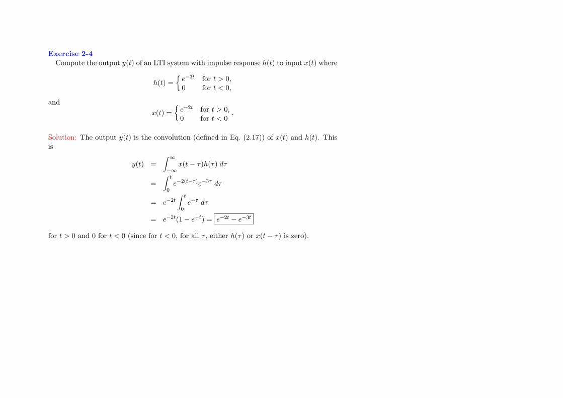
Exercise 2-4Compute the output y(t) of an LTI system with impulse response h(t) to input x(t) where

h(t) =e−3t for t > 0,0 for t < 0,

andx(t) =

e−2t for t > 0,0 for t < 0

.

Solution: The output y(t) is the convolution (defined in Eq. (2.17)) of x(t) and h(t). Thisis

y(t) =∫ ∞−∞

x(t− τ)h(τ) dτ

=∫ t

0e−2(t−τ)e−3τ dτ

= e−2t∫ t

0e−τ dτ

= e−2t(1− e−t) = e−2t − e−3t

for t > 0 and 0 for t < 0 (since for t < 0, for all τ , either h(τ) or x(t− τ) is zero).

22

Exercise 2-5A square wave x(t) has the Fourier series expansionx(t) = sin(t) + 1

3 sin(3t) + 15 sin(5t) + 1

7 sin(7t) + . . .

Compute output y(t) if x(t)→ h(t) = 0.4 sinc(0.4t) → y(t).

Solution: x(t) has components at 12π = 0.16 Hz, 3

2π = 0.48 Hz, 52π = 0.80 Hz, 7

2π = 1.12 Hz,. . .h(t) is the impulse response of an ideal lowpass filter Eq. (2.34) with cutoff frequency

fc = 0.2 Hz. Only the sinusoid at 0.2 Hz gets through the lowpass filter, so y(t) = sin(t)

23

Exercise 2-6Compute the Fourier transform of d

dtsinc(t).

Solution: From Eqs. (2.33), (2.34) and (2.35), FFFsinc(t) =j2πf for |f | < 0.50 for |f | > 0.5

(set fc = 0.5), and from entry #5 in Table 2-4, FFFdxdt = (j2πf) X(f).

Combining these gives FFF ddtsinc(t) =j2πf for |f | < 0.50 for |f | > 0.5

24

Exercise 2-7What is the Nyquist sampling rate for a signal bandlimited to 4 kHz?

Solution: From Section 2-4.1, the Nyquist rate is 2(4 kHz) = 8000 samples/s .

25

Exercise 2-8A 500 Hz sinusoid is sampled at 900 samples/s. No anti-alias filter is being used.What is the frequency of the reconstructed continuous-time sinusoid?

Solution: The spectrum of the sampled signal has components at frequencies±500,±900± 500,±1800± 500, . . . = ±400,±500,±1300,±1400, . . . Hz.The reconstruction filter is a lowpass filter with cutoff 1

2(900) = 450 Hz.This leaves components at ±400 Hz. The frequency of the reconstructed sinusoid is

400 Hz .

26

Exercise 2-9A 28-Hertz sinusoid is sampled at 100 samples/second. What is Ω0 for the resulting

discrete-time sinusoid? What is the period of the resulting discrete-time sinusoid?

Solution: From Eq. (2.62), Ω0 = 2π 28100 = 0.56π From Eq. (2.63), Ω0

2π = 2π0.56π = N

D = 257 .

The period is the numerator N = 25Check: cos(0.56π[n+ 25]) = cos(0.56πn+ [0.56π25]) = cos(0.56πn+ 14π) = cos(0.56πn).

27

Exercise 2-10Compute the output y[n] of a discrete-time LTI system with impulse response h[n] and

input x[n], where h[n] = 3, 1 and x[n] = 1, 2, 3, 4.

Solution: From Eq. (2.71d), the output is the convolution y[n] = h[n] ∗ x[n] =(3)(1), (3)(2) + (1)(1), (3)(3) + (1)(2), (3)(4) + (1)(3), (1)(4) = 3, 7, 11, 15, 4

28

Exercise 2-11Compute the DTFT of 4 cos(0.15πn+ 1).

Solution: 4 cos(0.15πn+ 1) = 2ej1ej0.15πn + 2e−j1e−j0.15πn. Now take DTFTs of this.Applying the modulation property entry #3 in Table #2-6 to entry #2 in Table #2-7

givesDTFT[AejΩ0t] = A2πδ((Ω− Ω0)), where δ((Ω− Ω0)) =

∑∞k=−∞ δ(Ω− 2πk − Ω0).

Using this twice gives DTFT[4 cos(0.15πn+1)]=4πej1δ((Ω−0.15))+4πe−j1δ((Ω+0.15)).

29

Exercise 2-12Compute the inverse DTFT of 4 cos(2Ω) + 6 cos(Ω) + j8 sin(2Ω) + j2 sin(Ω).

Solution: Using 2 cos(Ω) = ejΩ + e−jΩ and 2j sin(Ω) = ejΩ − e−jΩ,we can rewrite this as 4 cos(2Ω) + 6 cos(Ω) + j8 sin(2Ω) + j2 sin(Ω)= 2[ej2Ω + e−j2Ω] + 3[ejΩ + e−jΩ] + 4[ej2Ω − e−j2Ω] + 1[ejΩ − e−jΩ]= (2 + 4)ej2Ω + (3 + 1)ej2Ω + (3− 1)e−jΩ + (2− 4)e−j2Ω = 6ej2ω + 4ej2ω + 2e−jω− 2e−j2ω.Using the definition Eq. (2.73a) of DTFT, we can read off the inverse DTFT asDTFT−1[4 cos(2Ω) + 6 cos(Ω) + j8 sin(2Ω) + j2 sin(Ω)] = 6, 4, 0, 2,−2.

30

Exercise 2-13Compute the 4-point DFT of 4, 3, 2, 1.

Solution: From Eq. (2.89a), the DFT is X[k] =∑N−1n=0 x[n] e−j2πnk/N for k = 0, 1, . . . , N−1.

Here N = 4 so X[k] =∑3n=0 x[n] e−j2πnk/4 for k = 0, 1, 2, 3.

Since e−j2πnk/4 = (e−j2π/4)nk = (−j)nk, this becomesX[0] = 1x[0] + 1x[1] + 1x[2] + 1x[3] since k = 0→ (−j)n0 = 1.X[1] = 1x[0]− jx[1]− 1x[2] + jx[3] since k = 1→ (−j)n1 = (−j)n.X[2] = 1x[0]− 1x[1] + 1x[2]− 1x[3] since k = 2→ (−j)n2 = (−1)n.X[3] = 1x[0] + jx[1]− 1x[2]− jx[3] since k = 3→ (−j)n3 = ((−j)3)n = jn.Inserting x[0] = 4, x[1] = 3, x[2] = 2, x[3] = 1 givesX[0] = 4 + 3 + 2 + 1 = 10 and X[1] = 4− j3− 2 + j1 = 2− j2.X[2] = 4− 3 + 2− 1 = 02 and X[3] = 4 + j3− 2− j1 = 2 + j2.DFT[4, 3, 2, 1]= 10, 2− j2, 2, 2 + j2 X[3] = X∗[1] as required by conjugate symme-

try.

31

Exercise 3-1How does one tell whether an image displayed in color is a color or a false-color image?

Solution: False-color images should have colorbars to identify the numerical value associatedwith each color.

32

Exercise 3-2Which of the following images is separable: (a) 2-D impulse; (b) box; (c) disk.

Solution: 2-D impulse δ(x, y) = δ(x) δ(y) and box Eq. (3.2) are separable; disk Eq. (3.3) isnot separable.

33

Exercise 3-3Which of the following is invariant to rotation: (a) 2-D impulse; (b) box; (c) disk.

Solution: 2-D impulse and disk are invariant to rotation; box is not invariant to rotation.

34

Exercise 3-4The operation of a 2-D mirror is described by g(x, y) = f(−x,−y). Find its PSF.

Solution: h(x, y; ξ, η) = δ(x+ ξ, y + η) This is a good example of a non-LSI system.The superposition integral Eq. (3.14) is

g(x, y) =∫ ∫

f(ξ, η) h(x, y; ξ, η) dξ dη.

We need to find h(x, y; ξ, η) so that

g(x, y) = f(−x,−y) =∫ ∫

f(ξ, η) h(x, y; ξ, η) dξ dη.

By inspection, h(x, y; ξ, η) = δ(x+ ξ, y + η) works.

35

Exercise 3-5If g(x, y) = h(x, y) ∗ ∗f(x, y), what is 4h(x, y) ∗ ∗f(x− 3, y − 2) in terms of g(x, y)?

Solution: 4g(x− 3, y − 2) by shift and scaling properties of 1-D convolution (Table 2-3).

36

Exercise 3-6Why do f(x, y) and f(x− x0, y − y0) have the same magnitude spectrum |F(µ, ν)|?

Solution: Let g(x, y) = f(x− x0, y − y0). Then, from entry #3 in Table 3-1,

|G(µ, ν)| = |e−j2πµx0e−j2πνy0F(µ, ν)| = |e−j2πµx0e−j2πνy0 |F(µ, ν)| = |F(µ, ν)|.

37

Exercise 3-7Compute the 2-D CSFT of f(x, y) = e−πr

2, where r2 = x2 + y2, without using Bessel

functions. Hint: f(x, y) is separable.

Solution: f(x, y) = e−πr2

= e−πx2e−πy

2is separable, so Eq. (3.19) and entry #5 of Table

2-5 (see also entry #13 of Table 3-1) give F(µ, ν) = e−πµ2e−πν

2= e−π(µ2+ν2) = e−πρ

2.

38

Exercise 3-8The 1-D phase spectrum φ(µ) in Fig. 3-6(c) is either 0 or 180 for all µ. Yet the phase

of the 1-D CTFT of a real-valued function must be an odd function of frequency. How canthese two statements be reconciled?

Solution: A phase of 180 is equivalent to a phase of −180. Replacing 180 with −180

for µ < 0 in Fig. 3-6(c) makes the phase φ(µ) an odd function of µ.

39

Exercise 3-9An image is spatially bandlimited to 10 cycles/m in both x and y directions. What is

the minimum sampling length ∆s to avoid aliasing?

Solution: ∆s < 12B = 1

20m . This is the sampling theorem (see Sections 2-4 and 3-5).

40

Exercise 3-10The 2-D CSFT of a 2-D impulse is one, so it is not spatially bandlimited. Why is it

possible to sample an impulse?

Solution: In general, it isn’t. Using a sampling interval of ∆s, the impulse δ(x−x0, y− y0)will be missed unless x0 and y0 are both integer multiples of ∆s.

41

Exercise 3-11If g[n,m] = h[n,m] ∗ ∗f [n,m], what is 4h[n,m] ∗ ∗f [n− 3, m− 2] in terms of g[n,m]?

Solution: 4g[n− 3, m− 2] by shift and scaling properties of 1-D convolution (Table 2-6).

42

Exercise 3-12Compute

[1 11 1

]∗ ∗[

1 11 1

].

Solution: Following Example 3-1,

(1)

1 1 01 1 00 0 0

+ (1)

0 0 01 1 01 1 0

+ (1)

0 1 10 1 10 0 0

+ (1)

0 0 00 1 10 1 1

=

1 2 12 4 21 2 1

43

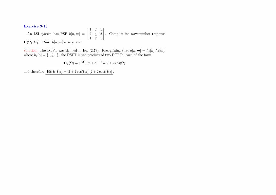
Exercise 3-13

An LSI system has PSF h[n,m] =

1 2 12 4 21 2 1

. Compute its wavenumber response

H(Ω1,Ω2). Hint: h[n,m] is separable.

Solution: The DTFT was defined in Eq. (2.73). Recognizing that h[n,m] = h1[n] h1[m],where h1[n] = 1, 2, 1, the DSFT is the product of two DTFTs, each of the form

H1(Ω) = ejΩ + 2 + e−jΩ = 2 + 2 cos(Ω)

and therefore H(Ω1,Ω2) = [2 + 2 cos(Ω1)][2 + 2 cos(Ω2)] .

44

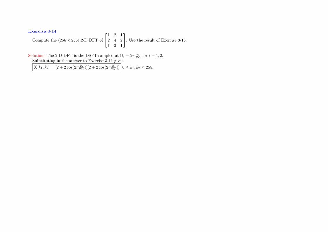
Exercise 3-14

Compute the (256× 256) 2-D DFT of

1 2 12 4 21 2 1

. Use the result of Exercise 3-13.

Solution: The 2-D DFT is the DSFT sampled at Ωi = 2π ki256 for i = 1, 2.

Substituting in the answer to Exercise 3-11 givesX[k1, k2] = [2 + 2 cos(2π k1

256)][2 + 2 cos(2π k2256)] 0 ≤ k1, k2 ≤ 255.

45

Exercise 3-15Why did this book not spend more space on computing the DSFT?

Solution: Because in practice, the DSFT is computed using the 2-D DFT.

46

Exercise 4-1If sinc interpolation is applied to the samples x(0.1n) = cos(2π(6)0.1n), what will be

the result?

Solution: x(0.1n) are samples of a 6 Hz cosine sampled at a rate of 10 samples/second.Sinc interpolation will be a cosine with frequency aliased to (10 − 6) = 4 Hz (see Section2-4.3).

47

Exercise 4-2Upsample the length-2 signal x[n] = 8, 4 to a length-4 signal y[n].

Solution: The 2-point DFT X[k] = 8 + 4, 8− 4 = 12, 4. Since N = 2 is even, we split4 and insert a zero in the middle, to get Y[k] = 12, 2, 0, 2. The inverse 4-point DFT is

y[0] =14

(12 + 2 + 0 + 2) = 4,

y[1] =14

(12 + 2j − 0− 2j) = 3,

y[2] =14

(12− 2 + 0− 2) = 2,

y[3] =14

(12− 2j + 0 + 2j) = 3.

Multiplying by 42 gives y[n] = 8, 6, 4, 6

48

Exercise 4-3Show that the area under βN (t) is one.

Solution:∫∞−∞ βN (t) dt = B(0) by entry #11 in Table 2-4.

Now set f = 0 in sincN (f) and use sinc(0)=1.

49

Exercise 4-4Why does βN (t) look like a Gaussian function for N ≥ 3?

Solution: Because βN (t) is rect(t) convolved with itself N+1 times. By the central limittheorem of probability, convolving any square-integrable function with itself results in afunction resembling a Gaussian.

50

Exercise 4-5Show that the support of βN (t) is −N+1

2 < t < N+12 .

Solution: The support of βN (t) is the interval outside of which βN (t) = 0. The support ofrect(t) is −1

2 < t < 12 . βN (t) is rect(t) convolved with itself N +1 times, which has duration

N + 1 centered at t = 0.

51

Exercise 4-6Given the samples x(0), x(∆), x(2∆), x(3∆) = 7, 4, 3, 2, compute x(∆/3) by interpo-

lation using: (a) nearest neighbor; (b) linear.

Solution: (a) ∆/3 is closer to 0 than to ∆, so x(∆/3) = x(0) = 7 .(b) x(∆/3) = 2

3x(0) + 13x(∆) = 2

3(7) + 13(4) = 6 .

52

Exercise 4-7In Eq. (4.63), why isn’t c[n] = x(n∆) for N ≥ 2?Answer: Because 3 of the basis functions βN

(t∆ −m

)overlap for any t. See Fig. 4-11.

53

Exercise 4-8The “image”

[1 23 4

]is interpolated using bilinear interpolation. What is the interpolated

value at the center of the image?

Solution: 14(1 + 2 + 3 + 4) = 2.5 .

54

Exercise 4-9The “image”

[1 23 4

]is rotated counter-clockwise 90. What is the result?

Solution:[

2 41 3

]This is pretty obvious.

55

Exercise 4-10The “image”

[4 812 16

]is magnified by a factor of three. What is the result, using: (a)

NN; (b) bilinear interpolation.

Solution: (a)

4 4 4 8 8 84 4 4 8 8 84 4 4 8 8 812 12 12 16 16 1612 12 12 16 16 1612 12 12 16 16 16

; (b)

1 2 1 2 4 22 4 2 4 8 41 2 1 2 4 23 6 3 4 8 46 12 6 8 16 83 6 3 4 8 4

.

Each of the 4 pixels of the original image is now the center of a (3× 3) array.

56

Exercise 5-1A star of magnitude six is barely visible to the naked eye in a dark sky. How much fainter

is a star of magnitude 6 than Vega, which has magnitude zero?

Solution: From Eq. (5.7), 106/2.512 = 244.6, so magnitude 6 is 245 times fainter than Vega.

57

Exercise 5-2What is another name for gamma transformation with γ = 1?

Solution: Linear transformation. Compare Eq. (5.10) and Eq. (5.1).

58

Exercise 5-3Show that the valid convolution of a Laplacian with a constant f [n,m] = c is zero.

Solution: Valid convolution (Section 5-2.5) is the usual convolution with edge effects omit-ted.

f ∗ ∗hLaplace = c1∑

n=−1

1∑m=−1

0 1 01 −4 10 1 0

= 0.

59

Exercise 5-4Perform histogram equalization on the (2× 2) “image”

[0.3 0.20.2 0.3

].

Solution: The histogram of the image is: 0.2 occurring twice and 0.3 occurring twice.The CDF is:

Pf (f0) =

0 for 0 ≤ f0 < 0.2,2 for 0.2 ≤ f0 < 0.3,4 for 0.3 ≤ f0 < 1.

Pixel value 0.2 is mapped to Pf (0.2) = 2 and pixel value 0.3 is mapped to Pf (0.3) = 4.

The histogram-equalized “image” is[

4 22 4

], which has a wider range of values than the

original.

60

Exercise 5-5Show that edge detection applied to a constant image f [n,m] = c gives no edges.

Solution: Valid convolution (Section 5-2.5) is the usual convolution with edge effects omit-ted.

The valid convolutions with hH[n,m] and hV[n,m] are defined in Eq. (5.49) and Eq. (5.51):

f ∗ ∗ hH = c1∑

n=−1

1∑m=−1

1 0 −12 0 −21 0 −1

= 0.

f ∗ ∗ hV = c1∑

n=−1

1∑m=−1

1 2 10 0 0−1 −2 −1

= 0.

Then the edge-direction gradient g[n,m] defined in Eq. (5.52) is zero.

61

Exercise 6-1Apply Tikhonov regularization with λ = 0.01 to the 1-D deconvolution problem x[0], x[1]∗h[0], h[1], h[2] = 2,−5, 4,−1, where h[0] = h[2] = 1 and h[1] = −2.

Solution: H(0) = 1− 2 + 1 = 0 so X(Ω) = Y(Ω)H(Ω) won’t work at Ω = 0, for any DFT order.

ButX(Ω) =

H∗(Ω)|H(Ω)|2 + λ2

Y(Ω)

does work.Using 4-point DFTs (computable by hand) gives

x[n] = 1.75,−1.25,−0.25,−0.25 ,

which is close to the actual x[n] = 2,−1. MATLAB:h=[1 -2 1];x=[2 -1];y=conv(x,h);H=fft(h,4);Y=fft(y);Z=conj(H).*Y./(abs(H).*abs(H)+0.0001);z=real(ifft2(Z)) provides the estimated

x[n].

62

Exercise 6-2For motion blur with a PSF of length N+1=60 in the direction of motion, at what spatial

frequencies Ω will the spatial frequency response be zero?

Solution: From Eq. (6.50), the numerator of the spatial frequency response is zero whenΩ = ±kπ/30 for any nonzero integer k.

63

Exercise 7-1(a) An input signal of duration N is fed into a tree-based filter bank of five stages. What

is the combined total duration of the output signals? Repeat for (b) an octave-based filterbank.

Solution: (a) 25N = 32N . (b) N since lower-wavenumber bands can be sampled less often.

64

Exercise 7-2A square wave x(t) has the Fourier series expansion x(t) =

∑∞k=1

1k sin(2πkt). x(t) is

passed through a brick-wall lowpass filter with cutoff frequency 2.5 Hz. What is the ratioof the average power of y(t) to the average power of x(t). Hint:

∑∞k=1

1k2 = π2

6 .

Solution: Rayleigh’s theorem relates average power to Fourier series coefficients.The average power of x(t) is

∑∞k=1

1k2 = π2

6 and the average power of y(t) is∑2k=1

1k2 =

1.25,since the lowpass filter has set the Fourier series coefficients for k ≥ 3 to zero.

1.25π2/6

= 0.76 .

65

Exercise 7-3Compute the cyclic convolution of 1, 2 and 3, 4 for N = 2.

Solution: Following Example 7-1, 1, 2 ∗ 3, 4 = 3, 10, 8. Aliasing gives 8 + 3, 10 =11, 10

66

Exercise 7-4x[n]→ ↑ 2 → ↓ 2 → y[n]. Express y[n] in terms of x[n].

Solution: y[n] = x[n] Zero-stuffing inserts zeros between consecutive values of x[n] anddecimating removes those zeros, leaving the original x[n].

67

Exercise 7-5If y[n] = h[n] ∗ x[n], what is h[n](−1)n ∗ x[n](−1)n in terms of y[n]?

Solution: From the “useful relation” Eq. (7.34), y[n](−1)n

68

Exercise 7-6Compute the one-stage Haar transform of x[n] =

√24, 3, 3, 4.

Solution: x[n] c© 1√2[1, 1] = 8, 7, 6, 7. Hence, xLD[n] = 8, 6 .

x[n] c© 1√2[1,−1] = 0,−1, 0, 1. Hence, xHD[n] = 0, 0 .

69

Exercise 7-7If h[n] = 1

5√

26, 2, h[2], 3, find h[2] so that h[n] satisfies the Smith-Barnwell condition.

Solution: According to Eq. (7.63), the Smith-Barnwell condition requires the autocorrela-tion of h[n] to be 1 for n = 0 and to be 0 for even n 6= 0.

For h[n] = a, b, c, d, these conditions give a2 + b2 + c2 + d2 = 1, ac+bd = 0, andh[2] = −1

70

Exercise 7-8What are the finest-detail signals of the db3 wavelet transform of x[n] = 3n2?

Solution: Zero. db3 wavelet basis function h[n] eliminates quadratic signals by construction.

71

Exercise 7-9Show by direct computation that the db2 scaling function listed in Table 7-3 satisfies the

Smith-Barnwell condition.

Solution: The Smith-Barnwell condition requires the autocorrelation of g[n] to be 1 for n = 0and to be 0 for even n 6= 0. For g[n] = a, b, c, d these conditions give a2 + b2 + c2 + d2 = 1and ac+bd = 0. The db2 g[n] listed in Table 7-3 is g[n] = 0.4830, 0.8365, [0.2241,−[0.1294.

It is easily verified that the sum of the squares of these numbers is 1, and that (0.4830)×(0.2241) + (0.8365)× (−0.1294) = 0.

72

Exercise 8-1For the coin flip experiment, what is the pmf for n = # flips of all tails followed by the

first head?

Solution: p[n] = a(1− a)(n−1) since we require n−1 consecutive tails before the first head.This is called a geometric pmf.

73

Exercise 8-2Given that the result of the coin flip experiment for N = 2 was one head and one tail,

compute P[H1].

Solution: There are 2 ways of getting one head and one tail: H1T2 and T1H2.Let P[Hi] = a so that P[Ti] = 1− a, and events B = H1 and C = H1T2 ∪ T1H2.Then B ∩ C = H1T2 and P[H1|H1T2 ∪ T1H2] = P[B|C] = P[B∩C]

P[C] = a(1−a)a(1−a)+a(1−a) = 1

2 .

74

Exercise 8-3Random variable x has the pdf

p(x) =

2x for 0 ≤ x ≤ 1,0 otherwise.

Compute P[x < 1/2].

Solution: P[x < 1/2] =∫ 1/2

0 2x dx = 1/4.

75

Exercise 8-4Random variable n has the pmf p[n] = (1

2)n for integers n ≥ 1. Compute P[n ≤ 5].

Solution: P[n ≤ 5] =∑5n=1(1

2)n = 31/32.

76

Exercise 8-5 In Example 8-6, compute the marginal pdf p(y) and conditional marginalpdf p(x|y).

Solution:p(y) =

∫ y

02 dx =

2y for 0 ≤ y ≤ 1,0 otherwise.

p(x|y) =p(x, y)p(y)

=

22y for 0 ≤ x < y ≤ 1,0 otherwise.

As expected, this becomes an impulse if y = 0.

77

Exercise 8-6In Example 8-7, compute the marginal pmf p[m] and conditional marginal pmf p[n|m].

Solution: p[m] =∑mn′=0

16 =

1/6 for m = 0,2/6 for m = 1,3/6 for m = 2.

Hence p[m] = m+16 for m = 0,1,2. p[n|m] = p[n,m]

p[m] = 1/6(m+1)/6 = 1

m+1 for m = 0,1,2, whichsums to 1.

78

Exercise 8-7In Example 8-6, compute (a) the mean E(y) and (b) variance σ2

y .

Solution: (a)

p(y) =∫ y

02 dx =

2y for 0 ≤ y ≤ 1,0 otherwise.

E[y] =∫ 1

0 y(2y) dy = 2/3

(b) E[y2] =∫ 1

0 y2(2y) dy = 1/2. Hence σ2

y = 12 − (2

3)2 = 118

79

Exercise 8-8Show that for the joint pdf given in Example 8-8, λx,y = 1

36 .

Solution: From Example 8-8(a), E[x] = 13 . Then:

E[xy] =∫ 1

0

∫ 1

x0

(x0y0)fx,y(x0, y0) dx0 dy0 = 2∫ 1

0x0 dx0

∫ 1

x0

y0 dy0 =∫ 1

0(x0 − x3

0) dx0 =14.

E[y] =∫ 1

0

∫ 1

x0

(y0)fx,y(x0, y0) dx0 dy0 = 2∫ 1

0dx0

∫ 1

x0

y0 dy0 =∫ 1

0(1− x2

0) dx0 =23.

λx,y = E[xy]− E[x]E[y] = 14 −

(13

) (23

)= 1

36

80

Exercise 8-9Random vector x has covariance matrix Kx =

[4 11 3

]. If y =

[4 32 1

]x, find Ky, Kx,y.

Solution:

Ky =[

4 32 1

] [4 11 3

] [4 32 1

]T=[

115 5151 23

],

Kx,y =[

4 32 1

] [4 11 3

]=[

19 139 5

].

81

Exercise 8-10A zero-mean WSS random process has power spectral density Sx(f) = 4

(2πf)2+4. What

is its autocorrelation function?

Solution: R(τ) = FFF−1Sx(f). From entry #3 in Table 2-5, R(τ) = e−2|τ |

82

Exercise 8-11A zero-mean WSS random process has the Gaussian autocorrelation function

R(τ) = e−πτ2.

What is its power spectral density?

Solution: Sx(f) = FFFR(τ). From entry #6 in Table 2-5, Sx(f) = e−πf2

83

Exercise 8-12x(t) is a white process with Rx(τ) = 5δ(τ) and y(t) =

∫ t+1t−1 x(τ) dτ , Compute the power

spectral density of y(t).

Solution: y(t) = rect(t/2) ∗ x(t). From entry #3 in Table #2-5, H(f) = FFFrect(t/2) =2 sinc(2f). So Sy(f) = |H(f)|2Sx(f) = 5(2 sinc(2f))2 = 20 sinc2(2f)

84

Exercise 8-13A white random field f(x, y) with auto-correlation function Rf (x, y) = 2δ(x) δ(y) is

filtered by an LSI system with PSF h(r) = 1r , where r is the radius in (x, y) space. Compute

the power spectral density of the output random field g(x, y).

Solution: From entry #5 in Table #3-2, H(ρ) = FFFh(r) = FFF1r = 1

ρ . Sf (µ, ν) = 2.

So Sg(µ, ν) = 2|H(ρ)|2 = 2ρ2

= 2µ2+ν2

85

Exercise 9-1How does Eq. (9.18) simplify when random vectors x and y are replaced with random

variables x and y?

Solution:xLS = x+

λx,yσ2y

(yobs − y).

Cross-covariance matrix Kx,y becomes covariance λx,y and covariance matrix Kx becomesvariance σ2

y .

86

Exercise 9-2Determine xLS and xMAP, given that only the a priori pdf p(x) is known.

Solution: xLS = x and xMAP = value of x maximizing p(x) .

Details:From Eq. (9.8), xLS = E[x|y = yobs ] = E[x] = x. p(yobs |x) is unknown since the

observation yobs is unknown. From Eq. (9.5), xMAP is the value of x maximizing p(x).

87

Exercise 9-3We observe random variable y whose pdf is p(y|λ) = λe−λy for y > 0. Compute the

maximum likelihood estimate of λ.

Solution: The log-likelihood function is log p(y|λ) = log λ− λyobs.

Setting its derivative to zero gives 1λ − yobs = 0. Solving, λMLE(yobs) =

1yobs

.

88

Exercise 9-4We observe random variable y whose pdf is p(y|λ) = λe−λy for y > 0 and λ has the a

priori pdf p(λ) = 3λ2 for 0 ≤ λ ≤ 1. Compute the maximum a posteriori estimate of λ.

Solution: The a posteriori pdf is

p(λ|y) =p(yobs|λ)p(λ)

p(yobs)= λe−λyobs

3λ2

p(yobs).

Its log is log λ − λyobs + log(3) + 2 log λ − log(p(yobs)). Setting its derivative to 0 gives3λ − yobs = 0.

Solving, λMAP(yobs) = 3/yobs if 3/yobs < 1, since λ < 1. Note λMAP(yobs) = 3λMLE(yobs).

89

Exercise 9-5Compute the MAP estimator for the coin-flip experiment assuming the a priori uniform

pdf p(x) = 1 for 0 ≤ x ≤ 1.

Solution: The algebra is the same as for computing xMLE. So xMAP = xMLE = nobs/N .

90

Exercise 9-6Compute the MAP estimator for the coin-flip experiment with N = 10 and the a priori

pdf p(x) = 3x2 for 0 ≤ x ≤ 1.

Solution: The a posteriori pdf is, modifying Eq. (9.28),

p(x|nobs) =3x2

C

xnobs(1− x)N−nobsN !

nobs!(N − nobs)!.

Taking the logarithm and omitting all terms independent of x gives

log p(x|nobs) = (nobs + 2) log x+ (N − nobs) log(1− x).

Setting the derivative to zero gives

0 =nobs + 2

x− N − nobs

1− x.

Solving for x gives

xMAP =nobs + 2N + 2

=nobs + 2

12.

91

Exercise 9-7Compute the MAP estimator for the coin-flip experiment with a triangular a priori pdf

p(x) = 2(1− x) for 0 ≤ x ≤ 1.

Solution: The a posteriori pdf is, modifying Eq. (9.28),

p(x|nobs) =2(1− x)

C

xnobs(1− x)N−nobsN !

nobs!(N − nobs)!.

Taking the logarithm and omitting all terms independent of x gives

log p(x|nobs) = (nobs) log x+ (N − nobs + 1) log(1− x).

Setting its derivative to zero gives

0 =nobs

x− N − nobs + 1

1− x.

Solving for x gives xMAP =nobs

N + 1.

Note that xMAP(nobs) < xMLE(nobs) as x is likely to be small, from the triangular a prioripdf.

92

Exercise 9-8Compute the mean and variance of the sample mean of N IID random variables xi,

each of which has mean x and variance σ2x.

Solution: From Chapter 8, the variance of the sum of uncorrelated random variables is thesum of their variances; independent random variables are uncorrelated, and σ2

ax = a2σ2x.

Let µ = 1N

∑Ni=1 xi be the sample mean of the xi. Then

σ2µ =

1N2

Nσ2x =

σ2x

M.

Also, E[µ] = 1N

∑Ni=1E[xi] = x, so the sample mean is an unbiased estimator of x.

So the sample mean converges to the actual mean x of the xi as M →∞.This is why the sample mean is useful, and why polling works.

93

Exercise 9-9What is MAP sparsifying estimator when noise variance σ2

v is much smaller than σx?

Solution: When σ2v σx, λ → 0 and xMAP = yobs from Eq. (9.82). This makes sense: if

the noise is low, use the observations whether or not they are a sparse estimate.

94

Exercise 9-10What is MAP sparsifying estimator when noise variance σ2

v is much greater than σx?

Solution: When σ2v σx, λ→∞, and xMAP = 0 from Eq. (9.82). This makes sense: the a

priori information that x is sparse dominates the noisy observation.

95

Exercise 9-11What happens to the stochastic Wiener filter when the observation noise σ2

v → 0?

Solution: In Eq. (9.93), letting σ2v → 0 results in RS(Ω) = Y(Ω)(1 − e−jΩ) whose inverse

DTFT is rs[n] = y[n]− y[n− 1] which is (noise-free) Eq. (9.84b).

96

Exercise 9-12When σf →∞, the Laplacian pdf given by Eq. (9.114) approaches the uniform distribu-

tion. What does the MAP estimate reduce to when σf →∞?

Solution: As σf →∞, λ→ 0, in which case fMAP[n,m]→ gobs[n,m] from Eq. (9.116).This makes sense: σf →∞ means the a priori sparseness information no longer holds,so we have no choice but to rely on the observation gobs[n,m].

97

Exercise 9-13Suppose we estimate the autocorrelation function Rx[n] of data x[n], n = 0, . . . , N − 1

using the sample mean over i of x[i] x[i− n], zero-padding x[n] as needed. Show thatthe DFT of Rx[n] is the periodogram (this is one reason why the periodogram works).

Solution:

Rx[n] =1N

N−1∑i=0

x[i] x[i− n] =1N

N−1∑i=0

x[i] x[−(n− i)] =1N

(x[n] ∗ x[−n]).

From entries #4 and #6 of Table 2-7, the DSFT of (x[n] ∗ x[−n]) is

X(Ω) X(−Ω) = X(Ω) X∗(Ω) = |X(Ω)|2,

which is the periodogram defined in Eq. (9.118) (recall that Ω is sampled at Ω = 2πk/N).

98

Exercise 10-1What should the output of imagesc(ones(3,3,3)) be?

Solution: A 3× 3 all white image (the combination of 3× 3 red, green and blue images).

99

Exercise 10-2An image has fR[n,m] = fG[n,m] = fB[n,m] = 1 for all [n,m]. What is its YIQ color

system representation?

Solution: fY[n,m] = 1 and fI[n,m] = fQ[n,m] = 0 for all [n,m], as discussed belowEq. (10.4).

100

Exercise 10-3Should gamma transformation be applied to images using the RGB or YIQ format?

Solution: YIQ format, because gamma transformation is nonlinear; applying it to an RGBimage would distort its colors.

101

Exercise 10-4Should linear transformation be applied to images using the RGB or YIQ format?

Solution: RGB format, since this is the color system used to display the transformed image.Linear transformation of YIQ images may result in gR[n,m], gG[n,m], gB[n,m] ≥ gmax inEq. (5.1), even though a linear transformation of linear transformation Eq. (5.1) is linear.

102

Exercise 10-5Can the colors of a deconvolved image differ from those of the original image?

Solution: Yes. Regularization can alter values of the reconstructed fR[n,m], gG[n,m],fB[n,m] image, and this will affect the colors. However, the effect is usually too slight tobe noticeable.

103

Exercise 10-6If the PSFs for different colors are different, can we still deconvolve the image?

Solution: Yes. Use the proper PSF for each color in Eq. (10.15).

104

Exercise 10-7If the length of the blur were N + 1 = 6, at what Ω1 values would H(Ω1,Ω2) = 0?

Solution: The numerator of Eq. (10.17) is zero when sin(Ω1(N + 1)/2) = 0, which occurswhen Ω1(N + 1)/2 is a multiple of π, or equivalently, when Ω1 = ±kπ/3 for integers k.

105

Exercise 11-1We have two classes of (1 × 1) images f1[n,m] = 1 and f2[n,m] = 4. Use correlation to

classify gobs[n,m] = 2.

Solution: ρ1 = (2)(1) = 2 and ρ2 = (2)(4) = 8. Since ρ2 > ρ1, classify gobs[n,m] as k = 2 .This is counter-intuitive (2 is closer to 1 than to 4), so see Exercise 11-2.

106

Exercise 11-2We have two classes of (1 × 1) images f1[n,m] = 1 and f2[n,m] = 4. Use the MLE

classifier to classify gobs[n,m] = 2.

Solution: ρ1 = (2)(1)=2 and ρ2 = (2)(4)=8. ΛMLE[1] = 2(2)−12 = 3 and ΛMLE[2] =2(8)−42 = 0. Since ΛMLE[1] > ΛMLE[2], classify gobs[n,m] as k = 1 .

Including energies of the images resulted in a different, and more intuitive, classification.

107

Exercise 11-3We have two classes of (1 × 1) images f1[n,m] = 1 and f2[n,m] = 4, with respective a

priori probabilities p[k = 1] = 0.1 and p[k = 2] = 0.9. The additive noise has σ2v = 3. Use

the MAP classifier to classify gobs[n,m] = 2.

Solution: ρ1 = (2)(1)=2 and ρ2 = (2)(4)=8.ΛMAP[1] = 2(2)−12+2(3) log(0.1) = −10.8.ΛMAP[2] = 2(4)−42+2(3) log(0.9) = −0.63.Since ΛMAP[2] > ΛMAP[1], classify gobs[n,m] as k = 2 .The a priori probabilities biased the classification towards k = 2.

108

Exercise 12-1Use a perceptron to implement a digital OR logic gate (y = x1 + x2, except 1 + 1 = 1).

Solution: Use Fig. 12-1(a) with φ(x) ≈ u(x), weights w1 = w2 = 1, and any w0 such that−1 < w0 < 0.

109

Exercise 12-2Use a perceptron to implement a digital AND logic gate (y = x1x2).

Solution: Use Fig. 12-1(a) with φ(x) ≈ u(x), weights w1 = w2 = 1, and any w0 such that−2 < w0 < −1.

110