October 16, 2003Doug JamesCarnegie Mellon University

http://www.cs.cmu.edu/~djames/15-462/Fall03

BlendingDisplay Color ModelsFiltersDitheringImage Compression

BlendingDisplay Color ModelsFiltersDitheringImage Compression

Image ProcessingImage Processing

15-462 Computer Graphics I

Lecture 15

10/16/2003 15-462 Graphics I 2

OutlineOutline

• Blending

• Display Color Models• Filters• Dithering

• Image Compression

10/16/2003 15-462 Graphics I 3

BlendingBlending

• Frame buffer– Simple color model: R, G, B; 8 bits each

– α-channel A, another 8 bits

• Alpha determines opacity, pixel-by-pixel– α = 1: opaque– α = 0: transparent

• Blend translucent objects during rendering

• Achieve other effects (e.g., shadows)

10/16/2003 15-462 Graphics I 4

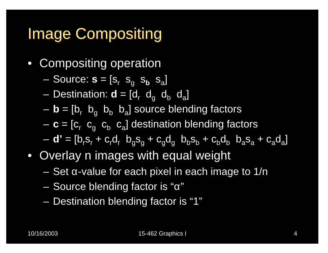
Image CompositingImage Compositing

• Compositing operation– Source: s = [sr sg sb sa]– Destination: d = [dr dg db da]– b = [br bg bb ba] source blending factors– c = [cr cg cb ca] destination blending factors– d’ = [brsr + crdr bgsg + cgdg bbsb + cbdb basa + cada]

• Overlay n images with equal weight– Set α-value for each pixel in each image to 1/n– Source blending factor is “α”– Destination blending factor is “1”

10/16/2003 15-462 Graphics I 5

Blending in OpenGLBlending in OpenGL

• Enable blending

• Set up source and destination factors

• Source and destination choices– GL_ONE, GL_ZERO

– GL_SRC_ALPHA, GL_ONE_MINUS_SRC_ALPHA

– GL_DST_ALPHA, GL_ONE_MINUS_DST_ALPHA

glEnable(GL_BLEND);

glBlendFunc(source_factor, dest_factor);

10/16/2003 15-462 Graphics I 6

Blending ErrorsBlending Errors

• Operations are not commutative

• Operations are not idempotent• Interaction with hidden-surface removal

– Polygon behind opaque one should be culled– Translucent in front of others should be composited– Solution:

• Two passes using alpha testing (glAlphaFunc): 1st pass alpha=1 accepted, and 2nd pass alpha<1 accepted

• make z-buffer read-only for translucent polygons (alpha<1) with glDepthMask(GL_FALSE);

10/16/2003 15-462 Graphics I 7

Antialiasing RevisitedAntialiasing Revisited

• Single-polygon case first

• Set α-value of each pixel to covered fraction• Use destination factor of “1 – α”• Use source factor of “α”• This will blend background with foreground• Overlaps can lead to blending errors

10/16/2003 15-462 Graphics I 8

Antialiasing with Multiple PolygonsAntialiasing with Multiple Polygons

• Initially, background color C0, α0 = 0

• Render first polygon; color C1fraction α1

– Cd = (1 – α1)C0 + α1C1

– αd = α1

• Render second polygon; assume fraction α2

• If no overlap (a), then– C’d = (1 – α2)Cd + α2C2

– α’d = α1 + α2

10/16/2003 15-462 Graphics I 9

Antialiasing with OverlapAntialiasing with Overlap

• Now assume overlap (b)

• Average overlap is α1α2

• So αd = α1 + α2 – α1α2

• Make front/back decision for color as usual

10/16/2003 15-462 Graphics I 10

Antialiasing in OpenGLAntialiasing in OpenGL

• Avoid explicit α-calculation in program• Enable both smoothing and blending

• Can also hint about quality vs performance using glHint(…)

glEnable(GL_POINT_SMOOTH);glEnable(GL_LINE_SMOOTH);glEnable(GL_BLEND);glBlendFunc(GL_SRC_ALPHA, GL_ONE_MINUS_SRC_ALPHA);

10/16/2003 15-462 Graphics I 11

Depth Cueing and FogDepth Cueing and Fog

• Another application of blending• Use distance-dependent (z) blending

– Linear dependence: depth cueing effect– Exponential dependence: fog effect– This is not a physically-based model

10/16/2003 15-462 Graphics I 12

Example: FogExample: Fog

• Fog in RGBA mode:C = fCi + (1-f)Cf

– f : depth-dependent fog factor

GLfloat fcolor[4] = {...};

glEnable(GL_FOG);

glFogf(GL_FOG_MODE, GL_EXP);

glFogf(GL_FOG_DENSITY, 0.5);

glFogfv(GL_FOG_COLOR, fcolor);

[Example: Fog Tutor]

10/16/2003 15-462 Graphics I 13

Example: Depth CueExample: Depth Cue

float fogColor[] = {0.0f, 0.0f, 0.0f, 1.0f};

gl.glEnable(GL_FOG);

gl.glFogi (GL_FOG_MODE, GL_LINEAR);

gl.glHint (GL_FOG_HINT, GL_NICEST); /* per pixel */

gl.glFogf (GL_FOG_START, 3.0f);

gl.glFogf (GL_FOG_END, 5.0f);

gl.glFogfv (GL_FOG_COLOR, fogColor);

gl.glClearColor(0.0f, 0.0f, 0.0f, 1.0f);

10/16/2003 15-462 Graphics I 14

OutlineOutline

• Blending

• Display Color Models• Filters• Dithering

• Image Compression

10/16/2003 15-462 Graphics I 15

Displays and FramebuffersDisplays and Framebuffers

• Image stored in memory as 2D pixel array, called framebuffer

• Value of each pixel controls color • Video hardware scans the framebuffer at 60Hz

• Depth of framebuffer is information per pixel– 1 bit: black and white display (cf. Smithsonian)– 8 bit: 256 colors at any given time via colormap– 16 bit: 5, 6, 5 bits (R,G,B), 216 = 65,536 colors– 24 bit: 8, 8, 8 bits (R,G,B), 224 = 16,777,216 colors

10/16/2003 15-462 Graphics I 16

Fewer Bits: Color-Index ModeFewer Bits: Color-Index Mode

• Colormaps typical for 8 bit framebuffer depth• With screen 1024 * 768 = 786432 = 0.75 MB• Each pixel value is index into colormap• Colormap is array of RGB values, 8 bits each• All 224 colors can be represented• Only 28 = 256 at a time• Poor approximation of full color• Who owns the colormap?• Colormap hacks: affect image w/o changing

framebuffer (only colormap)

10/16/2003 15-462 Graphics I 17

More Bits: Graphics HardwareMore Bits: Graphics Hardware

• 24 bits: RGB

• + 8 bits: A (α-channel for opacity)• + 16 bits: Z (for hidden-surface removal)• * 2: double buffering for smooth animation

• = 96 bits• For 1024 * 768 screen: 9 MB

10/16/2003 15-462 Graphics I 18

Image ProcessingImage Processing

• 2D generalization of signal processing

• Image as a two-dimensional signal• Point processing: modify pixels independently• Filtering: modify based on neighborhood

• Compositing: combine several images• Image compression: space-efficient formats• Other topics (not in this course)

– Image enhancement and restoration– Computer vision

10/16/2003 15-462 Graphics I 19

OutlineOutline

• Blending

• Display Color Models• Filters• Dithering

• Image Compression

10/16/2003 15-462 Graphics I 20

Point ProcessingPoint Processing

• Input: a(x,y); Output: b(x,y) = f(a(x,y))

• Useful for contrast adjustment, false colors• Examples for grayscale, 0 � v � 1

– f(v) = v (identity)– f(v) = 1-v (negate image)– f(v) = vp, p < 1 (brighten)– f(v) = vp, p > 1 (darken)

• Gamma correction compensatesmonitor brightness loss

v

f(v)

10/16/2003 15-462 Graphics I 21

Gamma Correction ExampleGamma Correction Example

Γ = 1.0; f(v) = v Γ = 0.5; f(v) = v1/0.5 = v2 Γ = 2.5; f(v) = v1/2.5 = v0.4

10/16/2003 15-462 Graphics I 22

Signals and FilteringSignals and Filtering

• Audio recording is 1D signal: amplitude(t)

• Image is a 2D signal: color(x,y)• Signals can be continuous or discrete• Raster images are discrete

– In space: sampled in x, y– In color: quantized in value

• Filtering: a mapping from signal to signal

10/16/2003 15-462 Graphics I 23

Linear and Shift-Invariant FiltersLinear and Shift-Invariant Filters

• Linear with respect to input signal

• Shift-invariant with respect to parameter• Convolution in 1D

– a(t) is input signal– b(s) is output signal– h(u) is filter– Shorthand: b = a � h ( = h � a, as an aside)

• Convolution in 2D

10/16/2003 15-462 Graphics I 24

Filters with Finite SupportFilters with Finite Support

• Filter h(u,v) is 0 except in given region

• Represent h in form of a matrix• Example: 3 � 3 blurring filter

• As function

• In matrix form

10/16/2003 15-462 Graphics I 25

Blurring FiltersBlurring Filters

• Average values of surrounding pixels

• Can be used for anti-aliasing• Size of blurring filter should be odd• What do we do at the edges and corners?

• For noise reduction, use median, not average– Eliminates intensity spikes– Non-linear filter

10/16/2003 15-462 Graphics I 26

Examples of Blurring FilterExamples of Blurring Filter

Original Image Blur 3x3 mask Blur 7x7 mask

10/16/2003 15-462 Graphics I 27

Example Noise ReductionExample Noise Reduction

Original image Image with noise Median filter (5x5?)

10/16/2003 15-462 Graphics I 28

Edge FiltersEdge Filters

• Discover edges in image

• Characterized by large gradient

• Approximate square root

• Approximate partial derivatives, e.g.

10/16/2003 15-462 Graphics I 29

Sobel FilterSobel Filter

• Edge detection filter, with some smoothing

• Approximate

• Sobel filter is non-linear– Square and square root (more exact computation)– Absolute value (faster computation)

10/16/2003 15-462 Graphics I 30

Sample Filter Computation Sample Filter Computation

• Part of Sobel filter, detects vertical edges

-1

-1-2

0

00

1

12

4

125252525252525

252525

25252525252525

252525

25252525252525

252525

25252525252525

252525

25252525252525

252525

0000000

000

0000000

000

0000000

000

0000000

000

0000000

000

a b

25252525252525

252525

0000000

000

0000000

00

0000000

000

0000000

000

25252525252525

252525

0000000

000

0000000

000

0000000

000

0000000

000 0

h

10/16/2003 15-462 Graphics I 31

Example of Edge FilterExample of Edge Filter

Original image Edge filter, then brightened

10/16/2003 15-462 Graphics I 32

OutlineOutline

• Blending

• Display Color Models• Filters• Dithering

• Image Compression

10/16/2003 15-462 Graphics I 33

DitheringDithering

• Compensates for lack of color resolution

• Give up spatial resolution for color resolution• Eye does spatial averaging• Black/white dithering to achieve gray scale

– Each pixel is black or white– From far away, color determined by fraction of white– For 3x3 block, 10 levels of gray scale

• glEnable(GL_DITHER)

10/16/2003 15-462 Graphics I 34

Halftone ScreensHalftone Screens

• Regular patterns create some artefacts– Avoid stripes– Avoid isolated pixels (e.g. on laser printer)– Monotonicity: keep pixels on at higher intensities

• Example of good 3�3 dithering matrix

– For intensity n, turn on pixels 0..n–1

10/16/2003 15-462 Graphics I 35

Floyd-Steinberg Error DiffusionFloyd-Steinberg Error Diffusion

• Approximation without fixed resolution loss

• Scan in raster order• At each pixel, draw least error output value• Divide error into 4 different fractions

• Add the error fractions into adjacent, unwritten pixels

7/16

3/16 5/16 1/16

10/16/2003 15-462 Graphics I 36

Floyd-Steinberg ExampleFloyd-Steinberg Example

Peter Anderson

Gray Scale Ramp

•Some worms

•Some checkerboards

•Enhance edges

10/16/2003 15-462 Graphics I 37

Floyd-Steinberg ExampleFloyd-Steinberg Example

10/16/2003 15-462 Graphics I 38

Color DitheringColor Dithering

• Example: 8 bit framebuffer– Set color map by dividing 8 bits into 3,3,2 for RGB– Blue is deemphasized since we see it less well

• Dither RGB separately– Works well with Floyd-Steinberg

• Assemble results into 8 bit index into colormap• Generally looks good

10/16/2003 15-462 Graphics I 39

OutlineOutline

• Blending

• Display Color Models• Filters• Dithering

• Image Compression

10/16/2003 15-462 Graphics I 40

Image CompressionImage Compression

• Exploit redundancy– Coding: some pixel values more common– Interpixel: adjacent pixels often similar– Psychovisual: some color differences imperceptible

• Distinguish lossy and lossless methods

10/16/2003 15-462 Graphics I 41

Some Image File FormatsSome Image File Formats

Good for printingHuge1,2,4,8,24EPS

Easy to read/writeBig24PPM

Popular, but 8 bitMedium1, 4, 8GIF

Good general purposeMedium8, 24TIFF

Lossy compressionSmall24JPEG

CommentsFile SizeDepth

10/16/2003 15-462 Graphics I 42

Image SizesImage Sizes

• 1024*1024 at 24 bits uses 3 MB

• Encyclopedia Britannica at 300 pixels/inch and 1 bit/pixel requires 25 gigabytes (25K pages)

• 90 minute movie at 640x480, 24 bits per pixels, 24 frames per second requires 120 gigabytes

• Applications: HDTV, DVD, satellite image transmission, medial image processing, fax, ...

10/16/2003 15-462 Graphics I 43

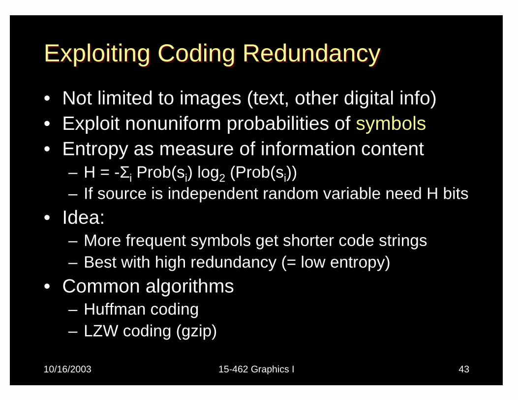
Exploiting Coding RedundancyExploiting Coding Redundancy

• Not limited to images (text, other digital info)• Exploit nonuniform probabilities of symbols• Entropy as measure of information content

– H = -Σi Prob(si) log2 (Prob(si))– If source is independent random variable need H bits

• Idea:– More frequent symbols get shorter code strings– Best with high redundancy (= low entropy)

• Common algorithms– Huffman coding– LZW coding (gzip)

10/16/2003 15-462 Graphics I 44

Huffman CodingHuffman Coding

• Codebook is precomputed and static– Use probability of each symbol to assign code– Map symbol to code– Store codebook and code sequence

• Precomputation is expensive• What is “symbol” for image compression?

10/16/2003 15-462 Graphics I 45

Lempel-Ziv-Welch (LZW) CodingLempel-Ziv-Welch (LZW) Coding

• Compute codebook on the fly

• Fast compression and decompression• Can tune various parameters• Both Huffman and LZW are lossless

10/16/2003 15-462 Graphics I 46

Exploiting Interpixel RedundancyExploiting Interpixel Redundancy

• Neighboring pixels are correlated• Spatial methods for low-noise image

– Run-length coding:• Alternate values and run-length• Good if horizontal neighbors are same• Can be 1D or 2D (e.g. used in fax standard)

– Quadtrees:• Recursively subdivide until cells are constant color

– Region encoding:• Represent boundary curves of color-constant regions

• Combine methods• Not good on natural images directly

10/16/2003 15-462 Graphics I 47

Improving Noise ToleranceImproving Noise Tolerance

• Predictive coding:– Predict next pixel based on prior ones– Output difference to actual

• Fractal image compression– Describe image via recursive affine transformation

• Transform coding– Exploit frequency domain– Example: discrete cosine transform (DCT)– Used in JPEG

• Transform coding for lossy compression

10/16/2003 15-462 Graphics I 48

Discrete Cosine TransformDiscrete Cosine Transform

• Used for lossy compression (as in JPEG)

• JPEG (Joint Photographic Expert Group)– Subdivide image into n � n blocks (n = 8)

– Apply discrete cosine transform for each block– Quantize, zig-zag order, run-length code coefficients– Use variable length coding (e.g. Huffman)

• Many natural images can be compressed to 4 bits/pixel with little visible error

10/16/2003 15-462 Graphics I 49

SummarySummary

• Display Color Models– 8 bit (colormap), 24 bit, 96 bit

• Filters– Blur, edge detect, sharpen, despeckle

• Dithering– Floyd-Steinberg error diffusion

• Image Compression– Coding, interpixel, psychovisual redundancy– Lossless vs. lossy compression

10/16/2003 15-462 Graphics I 50

PreviewPreview

• Assignment 5 due Thursday

• Assignment 6 out Thursday• Thursday: Ray Tracing