image patch analysis of sunspots and active regions
TRANSCRIPT
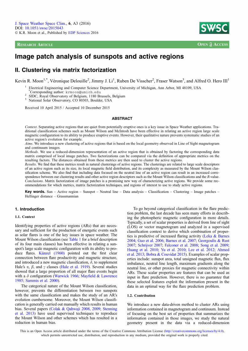
Image patch analysis of sunspots and active regions
II. Clustering via matrix factorization
Kevin R. Moon1,*, Véronique Delouille2, Jimmy J. Li1, Ruben De Visscher2, Fraser Watson3, and Alfred O. Hero III1
1 Electrical Engineering and Computer Science Department, University of Michigan, Ann Arbor, MI 48109, USA*Corresponding author: [email protected]
2 SIDC, Royal Observatory of Belgium, 1180 Brussels, Belgium3 National Solar Observatory, CO 80303, Boulder, USA
Received 10 April 2015 / Accepted 10 December 2015
ABSTRACT
Context. Separating active regions that are quiet from potentially eruptive ones is a key issue in Space Weather applications. Tra-ditional classification schemes such as Mount Wilson and McIntosh have been effective in relating an active region large scalemagnetic configuration to its ability to produce eruptive events. However, their qualitative nature prevents systematic studies of anactive region’s evolution for example.Aims. We introduce a new clustering of active regions that is based on the local geometry observed in Line of Sight magnetogramand continuum images.Methods. We use a reduced-dimension representation of an active region that is obtained by factoring the corresponding datamatrix comprised of local image patches. Two factorizations can be compared via the definition of appropriate metrics on theresulting factors. The distances obtained from these metrics are then used to cluster the active regions.Results. We find that these metrics result in natural clusterings of active regions. The clusterings are related to large scale descriptorsof an active region such as its size, its local magnetic field distribution, and its complexity as measured by the Mount Wilson clas-sification scheme. We also find that including data focused on the neutral line of an active region can result in an increased corre-spondence between our clustering results and other active region descriptors such as the Mount Wilson classifications and the R-value.Conclusions. Matrix factorization of image patches is a promising new way of characterizing active regions. We provide some rec-ommendations for which metrics, matrix factorization techniques, and regions of interest to use to study active regions.
Key words. Sun – Active region – Sunspot – Neutral line – Data analysis – Classification – Clustering – Image patches –Hellinger distance – Grassmannian
1. Introduction
1.1. Context
Identifying properties of active regions (ARs) that are neces-sary and sufficient for the production of energetic events suchas solar flares is one of the key issues in space weather. TheMount Wilson classification (see Table 1 for a brief descriptionof its four main classes) has been effective in relating a sun-spot’s large scale magnetic configuration with its ability to pro-duce flares. Künzel (1960) pointed out the first clearconnection between flare productivity and magnetic structure,and introduced a new magnetic classification, d, to supplementHale’s a, b, and c classes (Hale et al. 1919). Several studiesshowed that a large proportion of all major flare events beginwith a d configuration (Warwick 1966; Mayfield & Lawrence1985; Sammis et al. 2000).
The categorical nature of the Mount Wilson classification,however, prevents the differentiation between two sunspotswith the same classification and makes the study of an AR’sevolution cumbersome. Moreover, the Mount Wilson classifi-cation is generally carried out manually which results in humanbias. Several papers (Colak & Qahwaji 2008, 2009; Stenninget al. 2013) have used supervised techniques to reproducethe Mount Wilson and other schemes which has resulted in areduction in human bias.
To go beyond categorical classification in the flare predic-tion problem, the last decade has seen many efforts in describ-ing the photospheric magnetic configuration in more details.Typically, a set of scalar properties is derived from line of sight(LOS) or vector magnetogram and analyzed in a supervisedclassification context to derive which combination of proper-ties is predictive of increased flaring activity (Leka & Barnes2004; Guo et al. 2006; Barnes et al. 2007; Georgoulis & Rust2007; Schrijver 2007; Falconer et al. 2008; Song et al. 2009;Huang et al. 2010; Yu et al. 2010; Lee et al. 2012; Ahmedet al. 2013; Bobra & Couvidat 2015). Examples of scalar prop-erties include: sunspot area, total unsigned magnetic flux, fluximbalance, neutral line length, maximum gradients along theneutral line, or other proxies for magnetic connectivity withinARs. These scalar properties are features that can be used asinput in flare prediction. However, there is no guarantee thatthese selected features exploit the information present in thedata in an optimal way for the flare prediction problem.
1.2. Contribution
We introduce a new data-driven method to cluster ARs usinginformation contained in magnetogram and continuum. Insteadof focusing on the best set of properties that summarizes theinformation contained in those images, we study the naturalgeometry present in the data via a reduced-dimension
J. Space Weather Space Clim., 6, A3 (2016)DOI: 10.1051/swsc/2015043� K.R. Moon et al., Published by EDP Sciences 2016
OPEN ACCESSRESEARCH ARTICLE
This is an Open Access article distributed under the terms of the Creative Commons Attribution License (http://creativecommons.org/licenses/by/4.0),which permits unrestricted use, distribution, and reproduction in any medium, provided the original work is properly cited.
representation of such images. The reduced-dimension isimplemented via matrix factorization of an image patch repre-sentation as explained in Section 1.3. We show how this geom-etry can be used for classifying ARs in an unsupervised way,that is, without including AR labels as input to the analysis.
We consider the same dataset as in Moon et al. (2015). It isobtained from the Michelson Doppler Imager (MDI) instru-ment (Scherrer et al. 1995) on board the SOHO Spacecraft.SOHO-MDI provides two to four times per day a white-lightcontinuum image observed in the vicinity of the Ni I676.7L nm photospheric absorption line. MDI LOS magneto-grams are recorded with a higher nominal cadence of 96 min.We selected 424 sunspot images within the time range of1996–2010. They span the various Mount Wilson classifica-tions (see Table 1), are located within 30� of central meridian,and have corresponding observations in both MDI continuumand MDI LOS magnetogram. We use level 1.8 data for bothmodalities.
Our method can be adapted to any definition of the supportof an AR, or Region of Interest (ROI), and such ROI must begiven a priori. We consider three types of ROIs:
1. Umbrae and penumbrae masks obtained with theSunspot Tracking and Recognition Algorithm (STARA;Watson et al. 2011) from continuum images. Thesesunspot masks encompass the regions of highest varia-tion observed in both continuum and magnetogramimages, and hence are used primarily to illustrate ourmethod. Figure 1 provides some examples of AR imagesoverlaid with their respective STARA masks.
2. The neutral line region, defined as the set of pixels situ-ated no more than 10 pixels (20 arcsec) away from theneutral line, and located within the Solar Monitor ActiveRegion Tracker (SMART) masks (Higgins et al. 2011),which defines magnetic AR boundaries.
3. The set of pixels that are used as support for the compu-tation of the R-value defined in Schrijver (2007). TheR-value measures a weighted absolute magnetic flux,where the weights are positive only around the neutralline.
Our patch-based matrix factorization method investigatesthe fine scale structures encoded by localized gradients of var-ious directions and amplitudes, or locally smooth areas forexample. In contrast, the Mount Wilson classification encodesthe relative locations and sizes of concentrations of oppositepolarity magnetic flux on a large scale. Although both classifi-cation schemes rely on completely different methods, using thefirst ROI defined above, we find some similarities (see Sect. 5).Moreover, the Mount Wilson classification can guide us in theinterpretation of the results and clusters obtained.
The shape of the neutral line separating the two mainpolarities in an AR is a key element in the Mount Wilson
classification scheme, and the magnetic field gradientsobserved along the neutral line are important information inthe quest for solar activity prediction (Schrijver 2007; Falconeret al. 2008). We therefore analyze the effect of including theneutral line region in Section 5.
Results based on the third ROI are compared directly to theR-value. The various comparisons enable us to evaluate thepotential of our method for flare prediction.
1.3. Reduced dimension via matrix factorization
Our data-driven method is based on a reduced-dimension rep-resentation of an AR ROI via matrix factorization of imagepatches. Matrix factorization is a widely used tool to revealpatterns in high dimensional datasets. Applications outside ofsolar physics are numerous and range e.g. from multimediaactivity correlation, neuroscience, gene expression (Bazotet al. 2013), to hyperspectral imaging (Mittelman et al. 2012).
The idea is to express a k-multivariate observation z1 as alinear combination of a reduced number of r < k componentsaj, each weighted by some (possibly random) coefficients hj,1:
z1 ¼Xr
j¼1
ajhj;1 þ n1; ð1Þ
where n1 represents residual noise. With Z = [z1,. . ., zn], theequivalent matrix factorization representation is written as
Z ¼ AHþ N; ð2Þwhere Z is a k · n data matrix containing n observations of kdifferent variables, A is the k · r matrix containing the dic-tionary elements’ (called ‘‘factor loadings’’ in some applica-tions), and H is the r · n matrix of coefficients (or factorscores’). The k · n matrix N contains residuals from thematrix factorization model fitting. Finding A and H fromthe knowledge of Z alone is a severely ill-posed problem,hence prior knowledge is needed to constrain the solutionto be unique.
Principal Component Analysis (PCA; Jolliffe 2002) isprobably the most widely used dimensionality reduction tech-nique. It seeks principal directions that capture the highest var-iance in the data under the constraints that these directions aremutually orthogonal, thereby defining a subspace of the initialspace that exhibits information rather than noise. The PCAsolution can be written as a matrix factorization thanks tothe Singular Value Decomposition (SVD; Moon & Stirling2000), and so we use SVD in the clustering method presentedhere.
The Nonnegative Matrix Factorization (NMF; Lee &Seung 2001) is also considered in this paper. Instead of impos-ing orthogonality, it constrains elements of matrices A and Hto be nonnegative. We further impose that each column of Hhas elements that sum up to one, thereby effectively using a
Table 1. Mount Wilson classification rules, number of each AR, and total number of joint patches or pixels per Mount Wilson class used in thispaper when using the STARA masks.
Class Classification rule Numberof AR
Numberof patches
a A single dominant spot 50 13,358b A pair of dominant spots of opposite polarity 192 75,463bc A b sunspot where a single north-south polarity inversion line cannot divide the two polarities 130 95,631bcd A bc sunspot where umbrae of opposite polarity are together in a single penumbra 52 66,195
J. Space Weather Space Clim., 6, A3 (2016)
A3-p2
formulation identical to one used in hyperspectral unmixing(Bioucas-Dias et al. 2012).
Unmixing techniques exploit the high redundancyobserved in similar bandpasses. They aim at separating the var-ious contributions and at estimating a smaller set of less depen-dent source images. Matrix factorization, known as blindsource separation’ in this context, has many applications, rang-ing from biomedical imaging, chemometrics, to remote sens-ing (Comon & Jutten 2010), and recently to the extraction ofsalient morphological features from multiwavelength extremeultraviolet solar images (Dudok de Wit et al. 2013).
In this paper, we wish to factorize a k · n data matrix Zcontaining n observations of k different variables as inEq. (2) where the dictionary matrix A spans a subspace ofthe initial space, with r < k. We consider the cases where Zis formed from a single image as well as from multiple images.
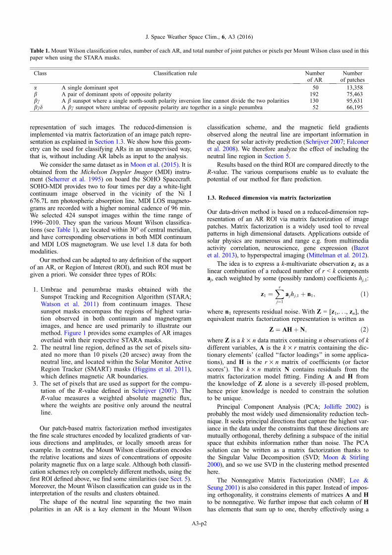
When a single image is used, the data matrix Z is builtfrom a n pixel image by taking overlapping m · m-pixel neigh-borhoods called patches. Figure 2a presents such a patch andits column representation. The k rows of the ith column of Zare thus given by the m2 pixel values in the neighborhood ofpixel i. The right plot in Figure 2 provides the number ofpatches in each pair of AR images when using the STARAmasks. When multiple images are used, such as when analyz-ing collectively all images from a given Mount Wilson class,the patches are combined into a single data matrix. Table 1gives the total number of patches from each Mount Wilsonclass when using the STARA masks.
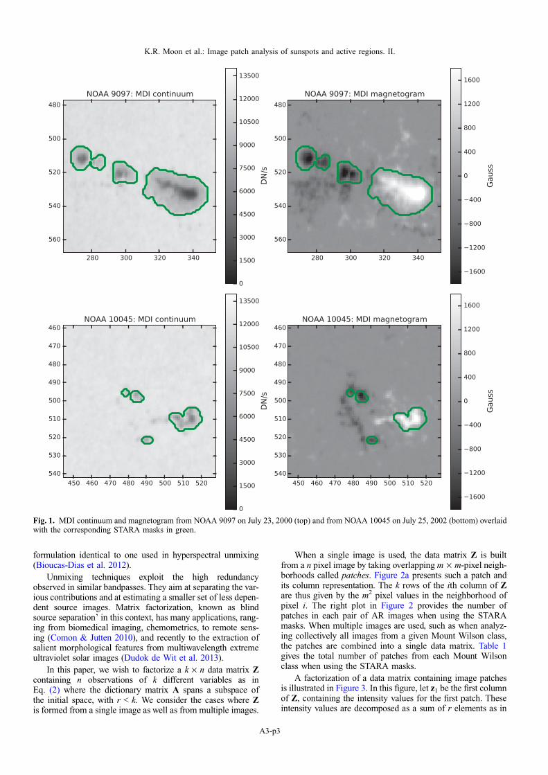
A factorization of a data matrix containing image patchesis illustrated in Figure 3. In this figure, let z1 be the first columnof Z, containing the intensity values for the first patch. Theseintensity values are decomposed as a sum of r elements as in
Fig. 1. MDI continuum and magnetogram from NOAA 9097 on July 23, 2000 (top) and from NOAA 10045 on July 25, 2002 (bottom) overlaidwith the corresponding STARA masks in green.
K.R. Moon et al.: Image patch analysis of sunspots and active regions. II.
A3-p3
Eq. (1) where aj is the jth column of A and hj,1 is the (j,1)thelement of H. In this representation, the vectors aj, j = 1,. . ., rare the elementary building blocks common to all patches,whereas the hj,1 are the coefficients specific to the first patch.
To compare ARs and cluster them based on this reduced-dimension representation, some form of distance is required.To measure the distance between two ARs, we apply somemetrics to the corresponding matrices A or H obtained fromthe factorizations of the two ARs. These distances are furtherintroduced into a clustering algorithm that groups ARs basedon the similarity of their patch geometry.
This paper builds upon results obtained in Moon et al.(2015), which can be summarized as follows:
1. Continuum and magnetogram modalities are correlated,and there may be some advantage in considering bothof them in an analysis.
2. A patch size of m = 3 includes a significant portion ofspatial correlations present in continuum and magneto-gram images.
3. Linear methods for dimensionality reduction (e.g. matrixfactorization) are appropriate to analyze ARs observedwith continuum images and magnetogram.
With an AR area equal to n pixels and an m · m patch, thecorresponding continuum data matrix X and magnetogramdata matrix Yeach have size m2 · n. The full data matrix con-
sidered is Z ¼ XY
� �with size 2m2 · n = 18 · n in our case.
The images extracted from both modalities are normalizedprior to analysis. An intrinsic dimension analysis in Moonet al. (2015) showed further that a sunspot can be representedaccurately with a dictionary containing six elements.
1.4. Outline
Section 2 describes two matrix factorization methods: the sin-gular value decomposition (SVD) and nonnegative matrix fac-torization (NMF). While more sophisticated methods exist thatmay lead to improved performance, we focus on SVD andNMF to demonstrate the utility of an analysis of a reduced-dimension representation of image patches for this problem.Future work will include further refinement in the choice ofmatrix factorization techniques. To compare the results fromthis factorization we need a metric, and so we use the Hellingerdistance for this purpose. To obtain some insight on how thesefactorizations separate the data, we make some general com-parisons in Section 3. In particular, with the defined metric,we compute the pairwise distances between Mount Wilsonclasses to identify which classes are most similar or dissimilaraccording to the matrix factorization results.
Section 4 describes the clustering procedures that take themetrics’ output as input. The method called Evidence Accu-mulating Clustering with Dual rooted Prim tree Cuts’ (EAC-DC) was introduced by Galluccio et al. (2013) and is used tocluster the ARs. By combining the two matrix factorizationmethods, a total of two procedures are used to analyze the data.Besides analyzing the whole sunspot data, we also look at
Fig. 2. (a) An example of a 3 · 3 pixel neighborhood or patch extracted from the edge of a sunspot in a continuum image and its columnrepresentation. (b) The number of patches extracted from each pair of AR images when using the STARA masks.
Fig. 3. An example of linear dimensionality reduction where the data matrix of AR image patches Z is factored as a product of a dictionary Aof representative elements and the corresponding coefficients in the matrix H. The A matrix consists of the basic building blocks for the datamatrix Z and H contains the corresponding coefficients.
J. Space Weather Space Clim., 6, A3 (2016)
A3-p4
information contained in patches situated along the neutrallines. The results of the clustering analyses are provided inSection 5.
This paper improves and extends the work in Moon et al.(2014), where fixed size square pixel regions centered on thesunspot group were used as the ROI for the matrix factoriza-tion prior to clustering. Moreover, here we are using moreappropriate metrics to compare the factorization results.
2. Matrix factorization
The intrinsic dimension analysis in Moon et al. (2015) showedthat linear methods (e.g. matrix factorization) are sufficient torepresent the data, and hence we focus on those. Matrix factor-ization methods aim at finding a set of basis vectors or dictio-nary elements such that each data point (in our case, pair ofpixel patches) can be accurately expressed as a linear combina-tion of the dictionary elements. Mathematically, if we usem · m patches then this can be expressed as Z � AH, whereZ is the 2m2 · n data matrix with n data points being consid-ered, A is the 2m2 · r dictionary with the columns correspond-ing to the dictionary elements, and H is the r · n matrix ofcoefficients. The goal is to find matrices A and H whose prod-uct nearly approximates Z. The degree of approximation istypically measured by the squared error jjZ� AHjj2F , where||Æ||F denotes the Frobenius norm (Yaghoobi et al. 2009). Addi-tional assumptions on the structure of the matrices A and Hcan be applied in matrix factorization depending on the appli-cation. Examples include assumptions of orthonormality of thecolumns of the dictionary A, sparsity of the coefficient matrixH (Ramírez & Sapiro 2012), and nonnegativity on A and H(Lin 2007).
We consider two popular matrix factorization methods: thesingular value decomposition (SVD) and nonnegative matrixfactorization (NMF).
2.1. Factorization using SVD
To perform matrix factorization using SVD, we take the singu-lar value decomposition of the data matrix Z = URVT, whereU is the matrix of the left singular vectors, R is a diagonalmatrix containing the singular values, and V is a matrix ofthe right singular vectors. If the size of the dictionary r is fixedand is less than 2m2, then the matrix of rank r that is closest toZ in terms of the Frobenius norm is the matrix productUrRrV
Tr , where Ur and Vr are matrices containing only the first
r singular vectors and Rr contains only the first r singular val-ues (Moon & Stirling 2000). Thus for SVD, the dictionary andcoefficient matrices are A = Ur and H ¼ RrV
Tr , respectively.
Note that SVD enforces orthonormality on the columns ofUr. Further details are included in Appendix A.1.
The intrinsic dimension estimated in Moon et al. (2015)determines the number of parameters required to accu-rately represent the data. It is used to provide an initial esti-mate for the size of the dictionaries r. For SVD, we chooser to be one standard deviation above the mean intrinsicdimension estimate, that is, r ’ 5 or 6. The choice of r isthen further refined by a comparison of dictionaries inSection 3. See Section 4.2 for more on selecting the dictio-nary size.
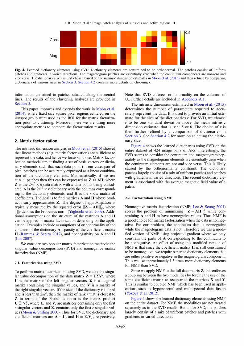
Figure 4 shows the learned dictionaries using SVD on theentire dataset of 424 image pairs of ARs. Interestingly, theSVD seems to consider the continuum and magnetogram sep-arately as the magnetogram elements are essentially zero whenthe continuum elements are not and vice versa. This is likelycaused by the orthonormality constraint. The dictionarypatches largely consist of a mix of uniform patches and patcheswith gradients in varied directions. The second dictionary ele-ment is associated with the average magnetic field value of apatch.
2.2. Factorization using NMF
Nonnegative matrix factorization (NMF; Lee & Seung 2001)solves the problem of minimizing jjZ� AHjj2F while con-straining A and H to have nonnegative values. Thus NMF isa good choice for matrix factorization when the data is nonneg-ative. For our problem, the continuum data is nonnegativewhile the magnetogram data is not. Therefore we use a modi-fied version of NMF using projected gradient where we onlyconstrain the parts of A corresponding to the continuum tobe nonnegative. An effect of using this modified version ofNMF is that since the coefficient matrix H is still constrainedto be nonnegative, we require separate dictionary elements thatare either positive or negative in the magnetogram component.Thus we use approximately 1.5 times more dictionary elementsfor NMF than SVD.
Since we apply NMF to the full data matrix Z, this enforcesa coupling between the two modalities by forcing the use of thesame coefficient matrix to reconstruct the matrices X and Y.This is similar to coupled NMF which has been used in appli-cations such as hyperspectral and multispectral data fusion(Yokoya et al. 2012).
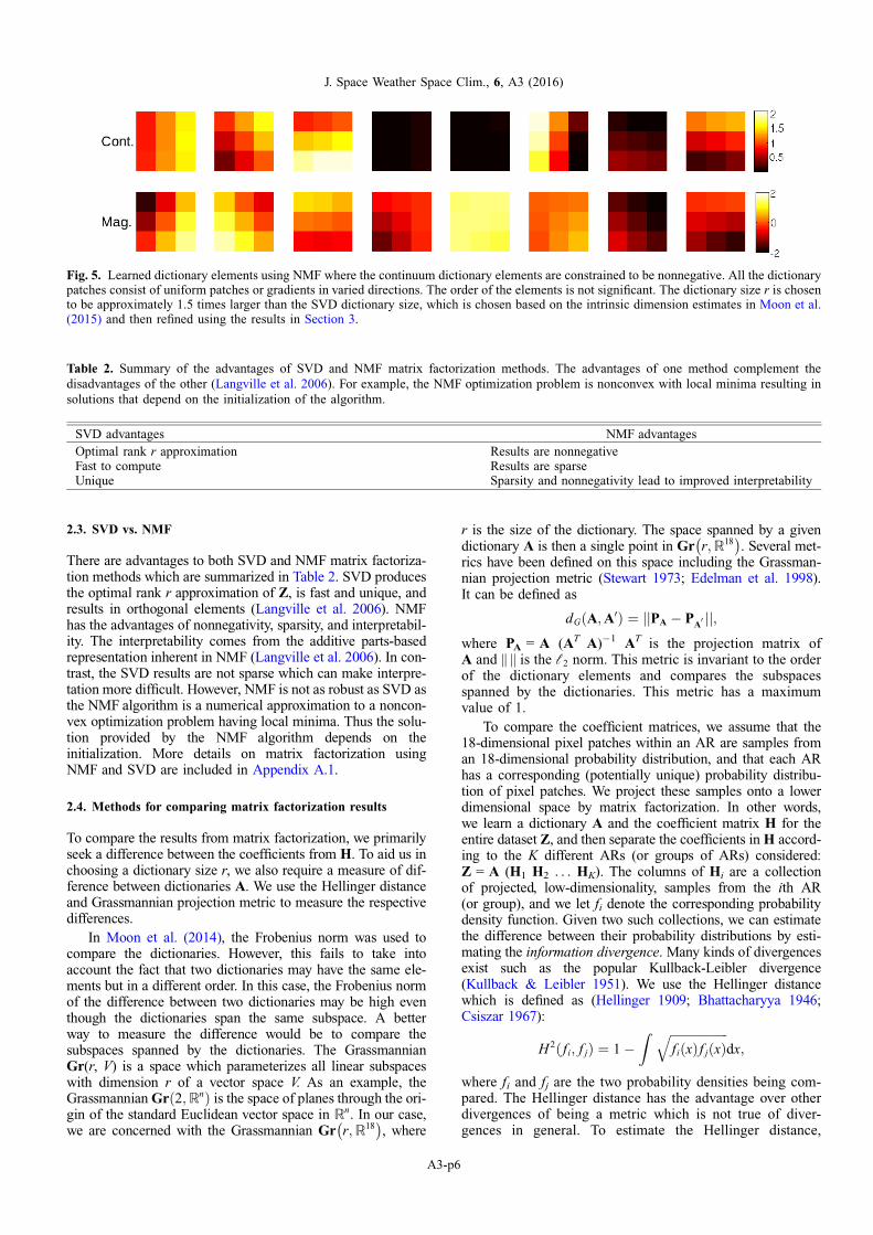
Figure 5 shows the learned dictionary elements using NMFon the entire dataset. For NMF, the modalities are not treatedseparately as in the SVD results. But as for SVD, the patcheslargely consist of a mix of uniform patches and patches withgradients in varied directions.
Fig. 4. Learned dictionary elements using SVD. Dictionary elements are constrained to be orthonormal. The patches consist of uniformpatches and gradients in varied directions. The magnetogram patches are essentially zero when the continuum components are nonzero andvice versa. The dictionary size r is first chosen based on the intrinsic dimension estimates in Moon et al. (2015) and then refined by comparingdictionaries of various sizes in Section 3. Section 4.2 contains more details on choosing r.
K.R. Moon et al.: Image patch analysis of sunspots and active regions. II.
A3-p5
2.3. SVD vs. NMF
There are advantages to both SVD and NMF matrix factoriza-tion methods which are summarized in Table 2. SVD producesthe optimal rank r approximation of Z, is fast and unique, andresults in orthogonal elements (Langville et al. 2006). NMFhas the advantages of nonnegativity, sparsity, and interpretabil-ity. The interpretability comes from the additive parts-basedrepresentation inherent in NMF (Langville et al. 2006). In con-trast, the SVD results are not sparse which can make interpre-tation more difficult. However, NMF is not as robust as SVD asthe NMF algorithm is a numerical approximation to a noncon-vex optimization problem having local minima. Thus the solu-tion provided by the NMF algorithm depends on theinitialization. More details on matrix factorization usingNMF and SVD are included in Appendix A.1.
2.4. Methods for comparing matrix factorization results
To compare the results from matrix factorization, we primarilyseek a difference between the coefficients from H. To aid us inchoosing a dictionary size r, we also require a measure of dif-ference between dictionaries A. We use the Hellinger distanceand Grassmannian projection metric to measure the respectivedifferences.
In Moon et al. (2014), the Frobenius norm was used tocompare the dictionaries. However, this fails to take intoaccount the fact that two dictionaries may have the same ele-ments but in a different order. In this case, the Frobenius normof the difference between two dictionaries may be high eventhough the dictionaries span the same subspace. A betterway to measure the difference would be to compare thesubspaces spanned by the dictionaries. The GrassmannianGr(r, V) is a space which parameterizes all linear subspaceswith dimension r of a vector space V. As an example, theGrassmannian Gr 2;Rnð Þ is the space of planes through the ori-gin of the standard Euclidean vector space in Rn. In our case,we are concerned with the Grassmannian Gr r;R18
� �, where
r is the size of the dictionary. The space spanned by a givendictionary A is then a single point in Gr r;R18
� �. Several met-
rics have been defined on this space including the Grassman-nian projection metric (Stewart 1973; Edelman et al. 1998).It can be defined as
dGðA;A0Þ ¼ jjPA � PA0 jj;
where PA = A (AT A)�1 AT is the projection matrix ofA and ||Æ|| is the l2 norm. This metric is invariant to the orderof the dictionary elements and compares the subspacesspanned by the dictionaries. This metric has a maximumvalue of 1.
To compare the coefficient matrices, we assume that the18-dimensional pixel patches within an AR are samples froman 18-dimensional probability distribution, and that each ARhas a corresponding (potentially unique) probability distribu-tion of pixel patches. We project these samples onto a lowerdimensional space by matrix factorization. In other words,we learn a dictionary A and the coefficient matrix H for theentire dataset Z, and then separate the coefficients in H accord-ing to the K different ARs (or groups of ARs) considered:Z = A (H1 H2 . . . HK). The columns of Hi are a collectionof projected, low-dimensionality, samples from the ith AR(or group), and we let fi denote the corresponding probabilitydensity function. Given two such collections, we can estimatethe difference between their probability distributions by esti-mating the information divergence. Many kinds of divergencesexist such as the popular Kullback-Leibler divergence(Kullback & Leibler 1951). We use the Hellinger distancewhich is defined as (Hellinger 1909; Bhattacharyya 1946;Csiszar 1967):
H 2ðfi; fjÞ ¼ 1�Z ffiffiffiffiffiffiffiffiffiffiffiffiffiffiffiffiffiffiffi
fiðxÞfjðxÞq
dx;
where fi and fj are the two probability densities being com-pared. The Hellinger distance has the advantage over otherdivergences of being a metric which is not true of diver-gences in general. To estimate the Hellinger distance,
Table 2. Summary of the advantages of SVD and NMF matrix factorization methods. The advantages of one method complement thedisadvantages of the other (Langville et al. 2006). For example, the NMF optimization problem is nonconvex with local minima resulting insolutions that depend on the initialization of the algorithm.
SVD advantages NMF advantagesOptimal rank r approximation Results are nonnegativeFast to compute Results are sparseUnique Sparsity and nonnegativity lead to improved interpretability
Fig. 5. Learned dictionary elements using NMF where the continuum dictionary elements are constrained to be nonnegative. All the dictionarypatches consist of uniform patches or gradients in varied directions. The order of the elements is not significant. The dictionary size r is chosento be approximately 1.5 times larger than the SVD dictionary size, which is chosen based on the intrinsic dimension estimates in Moon et al.(2015) and then refined using the results in Section 3.
J. Space Weather Space Clim., 6, A3 (2016)
A3-p6
we use the nonparametric estimator derived in Moon & HeroIII (2014a, 2014b) that is based on the k-nearest neighbordensity estimators for the densities fi and fj. This estimatoris simple to implement and achieves the parametric conver-gence rate when the densities are sufficiently smooth.
3. Comparisons of general matrix factorizationresults
We apply the metrics mentioned in Section 2.4 and comparethe local features as extracted by matrix factorization perMount Wilson class. One motivation for these comparisonsis to investigate differences between the Mount Wilson classesbased on the Hellinger distance. Another motivation is to fur-ther refine our choice of dictionary size r in preparation forclustering the ARs. When comparing the dictionary coeffi-cients using the Hellinger distance, we want a single, represen-tative dictionary that is able to accurately reconstruct all of theimages. Then the ARs will be differentiated based on theirrespective distributions of dictionary coefficients instead ofthe accuracy of their reconstructions. The coefficient distribu-tions can then be compared to interpret the clustering results asis done in Section 5.1.
Recall that our goal is to use unsupervised methods to sepa-rate the data based on the natural geometry. Our goal is not to rep-licate the Mount Wilson results. Instead we use the Mount Wilsonlabels in this section as a vehicle for interpreting the results.
3.1. Grassmannian metric comparisons
We first learn dictionaries for each of the Mount Wilson typesby applying matrix factorization to a subset of the patches
corresponding to sunspot groups of the respective type. Wethen use the Grassmannian metric to compare the dictionaries.For example, if we want to compare the a and b groups, wecollect a subset of patches from all ARs designated as a groupsinto a single data matrix Za. We then factor this matrix with thechosen method to obtain Za = Aa Ha. Similarly, we obtainZb = Ab Hb and then calculate dG (Aa, Ab).
The reason we use only a subset of patches is that each ARtype has a different number of total patches (see Table 1) whichmay introduce bias in the comparisons. One source of potentialbias in this case is due to the potentially increased patch vari-ability in groups with more patches, which would result inincreased difficulty in characterizing certain homogeneitiesof the patch features. This is mitigated somewhat by the factthat the local intrinsic dimension is typically less than 6 (Moonet al. 2015). However, it is possible that there may be differentlocal subspaces with the same dimension. A second source ofpotential bias is in the different levels of variance of the esti-mates due to difference in patch numbers. To circumvent thesepotential biases, we use the same number of patches in eachgroup for each comparison. For the interclass comparison,we randomly take 13,358 patches (the number of patches inthe smallest class) from each class to learn the dictionary,and then calculate the Grassmannian metric. For the intraclasscomparison, we take two disjoint subsets of 6679 patches (halfthe number of patches in the smallest class) from each class tolearn the dictionaries. This process is repeated 100 times andthe resulting mean and standard deviation are reported.
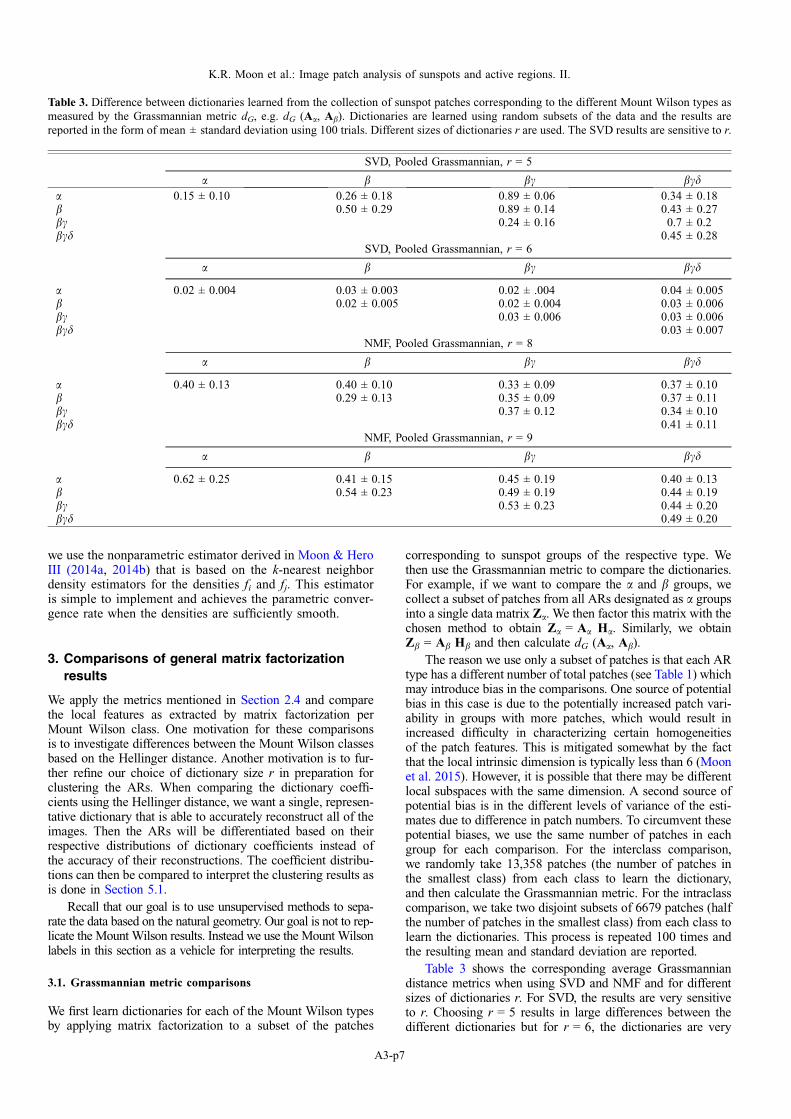
Table 3 shows the corresponding average Grassmanniandistance metrics when using SVD and NMF and for differentsizes of dictionaries r. For SVD, the results are very sensitiveto r. Choosing r = 5 results in large differences between thedifferent dictionaries but for r = 6, the dictionaries are very
Table 3. Difference between dictionaries learned from the collection of sunspot patches corresponding to the different Mount Wilson types asmeasured by the Grassmannian metric dG, e.g. dG (Aa, Ab). Dictionaries are learned using random subsets of the data and the results arereported in the form of mean ± standard deviation using 100 trials. Different sizes of dictionaries r are used. The SVD results are sensitive to r.
SVD, Pooled Grassmannian, r = 5
a b bc bcda 0.15 ± 0.10 0.26 ± 0.18 0.89 ± 0.06 0.34 ± 0.18b 0.50 ± 0.29 0.89 ± 0.14 0.43 ± 0.27bc 0.24 ± 0.16 0.7 ± 0.2bcd 0.45 ± 0.28
SVD, Pooled Grassmannian, r = 6
a b bc bcd
a 0.02 ± 0.004 0.03 ± 0.003 0.02 ± .004 0.04 ± 0.005b 0.02 ± 0.005 0.02 ± 0.004 0.03 ± 0.006bc 0.03 ± 0.006 0.03 ± 0.006bcd 0.03 ± 0.007
NMF, Pooled Grassmannian, r = 8
a b bc bcd
a 0.40 ± 0.13 0.40 ± 0.10 0.33 ± 0.09 0.37 ± 0.10b 0.29 ± 0.13 0.35 ± 0.09 0.37 ± 0.11bc 0.37 ± 0.12 0.34 ± 0.10bcd 0.41 ± 0.11
NMF, Pooled Grassmannian, r = 9
a b bc bcd
a 0.62 ± 0.25 0.41 ± 0.15 0.45 ± 0.19 0.40 ± 0.13b 0.54 ± 0.23 0.49 ± 0.19 0.44 ± 0.19bc 0.53 ± 0.23 0.44 ± 0.20bcd 0.49 ± 0.20
K.R. Moon et al.: Image patch analysis of sunspots and active regions. II.
A3-p7
similar. This suggests that for SVD, six principal componentsare sufficient to accurately represent the subspace upon whichthe sunspot patches lie. This is consistent with the results ofMoon et al. (2015) where the intrinsic dimension is found tobe less than 6 for most patches.
Interestingly, for the r = 5 SVD results, the bc group is themost dissimilar to the other groups while being relatively sim-ilar to itself. In contrast, the b group is fairly dissimilar to itselfand relatively similar to the a and bcd groups.
The NMF results are less sensitive to r. The average differ-ence between the dictionaries and its standard deviation is lar-ger when r = 9 compared to when r = 8. However, for a givenr, all of the mean differences are within a standard deviation ofeach other. Thus on aggregate, the NMF dictionaries learnedfrom large collections of patches from multiple images differfrom each other to the same degree regardless of the MountWilson type.
3.2. Hellinger distance comparisons
For the Hellinger distance, we learn a dictionary A and thecoefficient matrix H for the entire dataset Z. We then separatethe coefficients in H according to the Mount Wilson type andcompare the coefficient distributions using the Hellinger dis-tance. For example, suppose that the data matrix is arrangedas Z = (Za Zb Zbc Zbcd). This is factored as Z =A(Ha Hb Hbc Hbcd). To compare the a and b groups, weassume that the columns in Ha are samples from the distribu-tion fa and similarly Hb contains samples from the distributionfb. We then estimate the Hellinger distance H(fa, fb) using thedivergence estimator in Moon & Hero III (2014a).
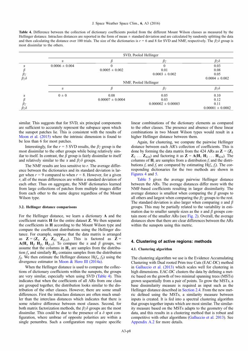
When the Hellinger distance is used to compare the collec-tions of dictionary coefficients within the sunspots, the groupsare very similar, especially when using SVD (Table 4). Thisindicates that when the coefficients of all ARs from one classare grouped together, the distribution looks similar to the dis-tribution of the other classes. However, there are some smalldifferences. First the intraclass distances are often much smal-ler than the interclass distances which indicates that there issome relative difference between most classes. Second, forboth matrix factorization methods, the bcd groups are the mostdissimilar. This could be due to the presence of a d spot con-figuration, where umbrae of opposite polarities are within asingle penumbra. Such a configuration may require specific
linear combinations of the dictionary elements as comparedto the other classes. The presence and absence of these linearcombinations in two Mount Wilson types would result in ahigher Hellinger distance between them.
Again, for clustering, we compute the pairwise Hellingerdistance between each AR’s collection of coefficients. This isdone by forming the data matrix from the 424 ARs as Z = (Z1
Z2 . . . Z424) and factoring it as Z = A(H1 H2 . . . H424). Thecolumns of Hi are samples from a distribution fi and the distri-butions fi and fj are compared by estimating H(fi, fj). The cor-responding dictionaries for the two methods are shown inFigures 4 and 5.
Table 5 gives the average pairwise Hellinger distancebetween the ARs. The average distances differ more with theNMF-based coefficients resulting in larger dissimilarity. Theaverage distance is smallest when comparing the b groups toall others and largest when comparing the bc groups to the rest.The standard deviation is also larger when comparing a and bgroups. This may be partially related to the variability in esti-mation due to smaller sample sizes as the a and b groups con-tain more of the smaller ARs (see Fig. 2). Overall, the averagedistances show that there are clear differences between the ARswithin the sunspots using this metric.
4. Clustering of active regions: methods
4.1. Clustering algorithm
The clustering algorithm we use is the Evidence AccumulatingClustering with Dual rooted Prim tree Cuts (EAC-DC) methodin Galluccio et al. (2013) which scales well for clustering inhigh dimensions. EAC-DC clusters the data by defining a met-ric based on the growth of two minimal spanning trees (MSTs)grown sequentially from a pair of points. To grow the MSTs, abase dissimilarity measure is required as input such as theHellinger distance described in Section 2.4. From the new met-ric defined using the MSTs, a similarity measure betweeninputs is created. It is fed into a spectral clustering algorithmthat groups together inputs which are most similar. The similar-ity measure based on the MSTs adapts to the geometry of thedata, and this results in a clustering method that is robust andcompetitive with other algorithms (Galluccio et al. 2013). SeeAppendix A.2 for more details.
Table 4. Difference between the collection of dictionary coefficients pooled from the different Mount Wilson classes as measured by theHellinger distance. Intraclass distances are reported in the form of mean ± standard deviation and are calculated by randomly splitting the dataand then calculating the distance over 100 trials. The size of the dictionaries is r = 6 and 8 for SVD and NMF, respectively. The bcd group ismost dissimilar to the others.
SVD, Pooled Hellinger
a b bc bcda 0.0006 ± 0.004 0 0 0.03b 0.0005 ± 0.002 0.01 0.08bc 0.0003 ± 0.002 0.05bcd 0.0004 ± 0.002
NMF, Pooled Hellinger
a b bc bcd
a 0 ± 0 0.08 0.05 0.10b 0.00007 ± 0.0004 0.03 0.12bc 0.000002 ± 0.00003 0.11bcd 0.00001 ± 0.0002
J. Space Weather Space Clim., 6, A3 (2016)
A3-p8
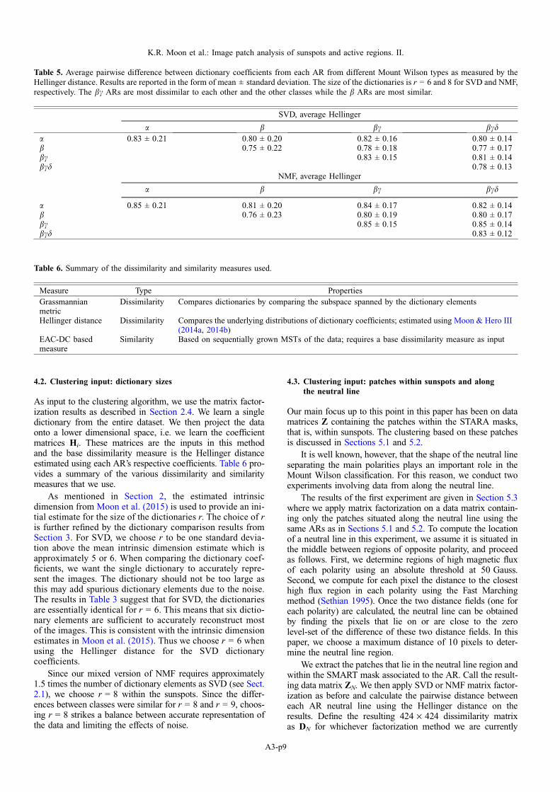
4.2. Clustering input: dictionary sizes
As input to the clustering algorithm, we use the matrix factor-ization results as described in Section 2.4. We learn a singledictionary from the entire dataset. We then project the dataonto a lower dimensional space, i.e. we learn the coefficientmatrices Hi. These matrices are the inputs in this methodand the base dissimilarity measure is the Hellinger distanceestimated using each AR’s respective coefficients. Table 6 pro-vides a summary of the various dissimilarity and similaritymeasures that we use.
As mentioned in Section 2, the estimated intrinsicdimension from Moon et al. (2015) is used to provide an ini-tial estimate for the size of the dictionaries r. The choice of ris further refined by the dictionary comparison results fromSection 3. For SVD, we choose r to be one standard devia-tion above the mean intrinsic dimension estimate which isapproximately 5 or 6. When comparing the dictionary coef-ficients, we want the single dictionary to accurately repre-sent the images. The dictionary should not be too large asthis may add spurious dictionary elements due to the noise.The results in Table 3 suggest that for SVD, the dictionariesare essentially identical for r = 6. This means that six dictio-nary elements are sufficient to accurately reconstruct mostof the images. This is consistent with the intrinsic dimensionestimates in Moon et al. (2015). Thus we choose r = 6 whenusing the Hellinger distance for the SVD dictionarycoefficients.
Since our mixed version of NMF requires approximately1.5 times the number of dictionary elements as SVD (see Sect.2.1), we choose r = 8 within the sunspots. Since the differ-ences between classes were similar for r = 8 and r = 9, choos-ing r = 8 strikes a balance between accurate representation ofthe data and limiting the effects of noise.
4.3. Clustering input: patches within sunspots and alongthe neutral line
Our main focus up to this point in this paper has been on datamatrices Z containing the patches within the STARA masks,that is, within sunspots. The clustering based on these patchesis discussed in Sections 5.1 and 5.2.
It is well known, however, that the shape of the neutral lineseparating the main polarities plays an important role in theMount Wilson classification. For this reason, we conduct twoexperiments involving data from along the neutral line.
The results of the first experiment are given in Section 5.3where we apply matrix factorization on a data matrix contain-ing only the patches situated along the neutral line using thesame ARs as in Sections 5.1 and 5.2. To compute the locationof a neutral line in this experiment, we assume it is situated inthe middle between regions of opposite polarity, and proceedas follows. First, we determine regions of high magnetic fluxof each polarity using an absolute threshold at 50 Gauss.Second, we compute for each pixel the distance to the closesthigh flux region in each polarity using the Fast Marchingmethod (Sethian 1995). Once the two distance fields (one foreach polarity) are calculated, the neutral line can be obtainedby finding the pixels that lie on or are close to the zerolevel-set of the difference of these two distance fields. In thispaper, we choose a maximum distance of 10 pixels to deter-mine the neutral line region.
We extract the patches that lie in the neutral line region andwithin the SMART mask associated to the AR. Call the result-ing data matrix ZN. We then apply SVD or NMF matrix factor-ization as before and calculate the pairwise distance betweeneach AR neutral line using the Hellinger distance on theresults. Define the resulting 424 · 424 dissimilarity matrixas DN for whichever factorization method we are currently
Table 6. Summary of the dissimilarity and similarity measures used.
Measure Type PropertiesGrassmannianmetric
Dissimilarity Compares dictionaries by comparing the subspace spanned by the dictionary elements
Hellinger distance Dissimilarity Compares the underlying distributions of dictionary coefficients; estimated using Moon & Hero III(2014a, 2014b)
EAC-DC basedmeasure
Similarity Based on sequentially grown MSTs of the data; requires a base dissimilarity measure as input
Table 5. Average pairwise difference between dictionary coefficients from each AR from different Mount Wilson types as measured by theHellinger distance. Results are reported in the form of mean ± standard deviation. The size of the dictionaries is r = 6 and 8 for SVD and NMF,respectively. The bc ARs are most dissimilar to each other and the other classes while the b ARs are most similar.
SVD, average Hellinger
a b bc bcda 0.83 ± 0.21 0.80 ± 0.20 0.82 ± 0.16 0.80 ± 0.14b 0.75 ± 0.22 0.78 ± 0.18 0.77 ± 0.17bc 0.83 ± 0.15 0.81 ± 0.14bcd 0.78 ± 0.13
NMF, average Hellinger
a b bc bcd
a 0.85 ± 0.21 0.81 ± 0.20 0.84 ± 0.17 0.82 ± 0.14b 0.76 ± 0.23 0.80 ± 0.19 0.80 ± 0.17bc 0.85 ± 0.15 0.85 ± 0.14bcd 0.83 ± 0.12
K.R. Moon et al.: Image patch analysis of sunspots and active regions. II.
A3-p9
using. Similarly, define ZS and DS as the respective data matrixand dissimilarity matrix of the data from within the sunspotsusing the same configuration. The base dissimilarity measureD inputted in the clustering algorithm is now a weighted aver-age of the distances computed within the neutral line regionsand within the sunspots: D = wDN + (1 � w)DS where0 � w � 1. Using a variety of weights, we then compare theclustering output to different labeling schemes based on theMount Wilson labels as shown in Table 7.
For the second experiment, we perform clustering on a ROIthat selects pixels along a strong field polarity reversal line.The high gradients near strong field polarity reversal lines inLOS magnetograms are a proxy for the presence of near-photospheric electrical currents, and thus might be indicativeof a nonpotential configuration (Schrijver 2007). To computethis ROI, the magnetograms are first reprojected using anequal-area, sinusoidal reprojection that uses Singular-ValuePadding (DeForest 2004). The latter is known to be more accu-rate than image interpolation on transformed coordinates. Toconserve flux, the magnetograms are also area-normalized.
In the reprojected magnetograms, we delimit an AR usingsunspot information from the Debrecen catalog (Györi et al.2010) to obtain the location of all the pixels that belong tothe spots related to an AR (called ‘‘Debrecen spots’’ hereafter).The ROI consists of a binary array constructed as follows:
1. The pixels that belong to the Debrecen spots are assignedthe scalar value 1 and all others are assigned the scalarvalue �1.
2. From this two-valued array, we retrieve the distancesfrom the zero level-set using a fast marching method(Sethian 1995) implemented in the Python SciKits’ mod-ule ‘‘scikit-fmm’’.
3. We mask out the pixels within a distance of 80 pixelsfrom the zero level-set (in the equal-area-reprojectedcoordinate system).
4. The ROI is delimited by the convex hull of the resultingmask, that is, the smallest convex polygon that surroundsall 1-valued pixels. The resulting mask is a binary arraywith the pixels inside the convex hull set to True.
Within the ROI, the R-value is calculated similarly to themethod described in Schrijver (2007). We dilate the imageusing a dilation factor of three pixels, and extract the flux usingoverlapping Gaussian masks with r = 2 px. Integrating thenonzero values outputs the R-value, i.e, the total flux in thevicinity of the polarity-inversion line.
We then perform an image patch analysis using imagepatches from this region. We do this by using either SVD orNMF to do dimensionality reduction on the patches, and thenestimate the Hellinger distance between ARs using thereduced-dimension representation. We exclude a groups fromthe analysis as they do not have a strong field polarity reversalline. This leaves 420 images to be clustered. The clustering
assignments are then compared to the calculated R-value viathe correlation coefficient. The results are presented inSection 5.4.
5. Clustering of active regions: results
Given the choices of matrix factorization techniques (NMF andSVD) we have two different clustering results on the data.Section 5.1 focuses on the clusterings using data from withinthe sunspots, and Section 5.2 provides some recommendationsfor which metrics and matrix factorization techniques to use tostudy different ARs. The neutral line clustering results are thengiven in Section 5.3 followed by the R-value based experimentin Section 5.4.
5.1. Clustering within the sunspot
We now present the clustering results when using the Hellingerdistance as the base dissimilarity. The corresponding dictionaryelements to the coefficients are represented in Figure 4 (for theSVD factorization) and in Figure 5 (for the NMF).
The EAC-DC algorithm does not automatically choose thenumber of clusters. We use the mean silhouette heuristic todetermine the most natural number of clusters as a functionof the data (Rousseeuw 1987). The silhouette is a measureof how well a data point belongs to its assigned cluster. Theheuristic chooses the number of clusters that results in themaximum mean silhouette. In both clustering configurations,the number of clusters that maximizes the mean silhouette is2 so we focus on the two clustering case for all clusteringschemes throughout.
To compare the clustering correspondence, we use theadjusted Rand index (ARI). The ARI is a measure of similaritybetween two clusterings (or a clustering and labels) and takesvalues between �1 and 1. A 1 indicates perfect agreementbetween the clusterings and a 0 corresponds to the agreementfrom a random assignment (Rand 1971). Thus a positive ARIindicates that the clustering correspondence is better than arandom clustering while a negative ARI indicates it is worse.The ARI between the NMF and SVD clusterings is 0.27 whichindicates some overlap.
Visualizing the clusters in lower dimensions is done withmultidimensional scaling (MDS) as in Moon et al. (2014).Let S be the 424 · 424 symmetric matrix that contains theAR pair similarities as created by EAC-DC algorithm. MDSprojects the similarity matrix S onto the eigenvectors of thenormalized Laplacian of S (Kruskal & Wish 1978). Letci 2 R424 be the projection onto the ith eigenvector of S usingNMF. The first eigenvector represents the direction of highestvariability in the matrix S, and hence a high value of the kthelement of c1 indicates that the kth AR is dissimilar to otherARs.
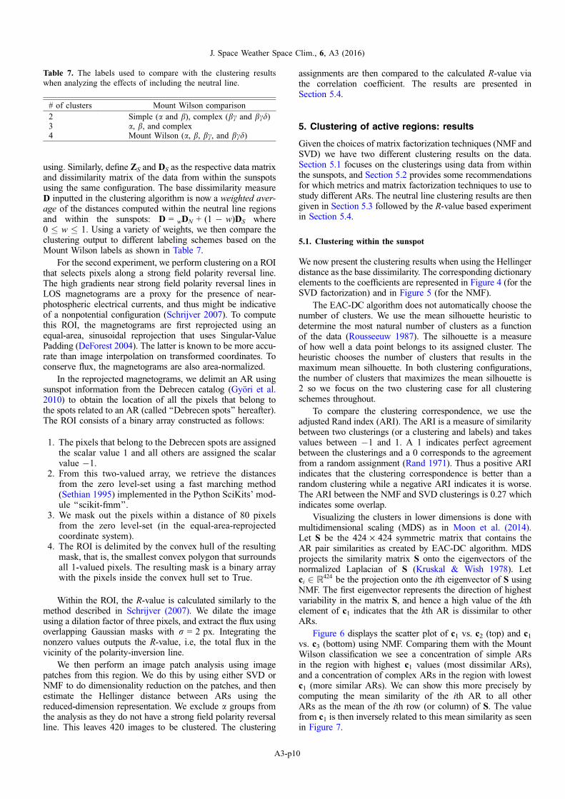
Figure 6 displays the scatter plot of c1 vs. c2 (top) and c1
vs. c3 (bottom) using NMF. Comparing them with the MountWilson classification we see a concentration of simple ARsin the region with highest c1 values (most dissimilar ARs),and a concentration of complex ARs in the region with lowestc1 (more similar ARs). We can show this more precisely bycomputing the mean similarity of the ith AR to all otherARs as the mean of the ith row (or column) of S. The valuefrom c1 is then inversely related to this mean similarity as seenin Figure 7.
Table 7. The labels used to compare with the clustering resultswhen analyzing the effects of including the neutral line.
# of clusters Mount Wilson comparison2 Simple (a and b), complex (bc and bcd)3 a, b, and complex4 Mount Wilson (a, b, bc, and bcd)
J. Space Weather Space Clim., 6, A3 (2016)
A3-p10
The similarity defined under this clustering scheme gathersin Cluster 2 ‘‘similar’’ ARs that are for a large part of the typesbc and bcd, whereas Cluster 1 contains ARs that are more dis-similar’ to each other, with a large part of a or b active regions.
The other clustering configuration has a similar relationshipbetween the first MDS coefficient and the mean similarity.
Table 8 makes this clearer by showing the mean similaritymeasure within each cluster and between the two clusters,which is calculated in the following manner. Suppose thatthe similarity matrix is organized in block form where theupper left block corresponds to Cluster 1 and the lower rightblock corresponds to Cluster 2. The mean similarity ofCluster 1 is calculated by taking the mean of all the values inthe upper left block of this reorganized similarity matrix. Themean similarity of Cluster 2 is found similarly from the lowerright block and the mean similarity between the clusters is foundfrom either the lower left or upper right blocks. These meansshow that under the NMF clustering scheme, ARs in Cluster 2
Fig. 6. Scatter plot of MDS variables c1 vs. c2 (a, b) and c1 vs. c3 (c, d) where ci 2 R424 is the projection of the similarity matrix onto the itheigenvector of the normalized Laplacian of the similarity matrix when using the NMF coefficients. Each point corresponds to one AR and theyare labeled according to the clustering (a, c) and the Mount Wilson labels (b, d). In this space, the clusters data appear to be separable and thereare concentrations of complex ARs in the region with lowest c1 values. Other patterns are described in the text.
Fig. 7. Mean similarity of an AR with all other ARs as a function ofits MDS variable c1 using NMF. Cluster 2 is associated with thoseARs that are most similar to all other ARs while Cluster 1 containsthose that are least similar to all others.
Table 8. Mean similarity of ARs to other ARs either in the samecluster (1 vs. 1 or 2 vs. 2) or in the other cluster (1 vs. 2) under thedifferent schemes. Cluster 1 contains ARs that are very dissimilar toeach other while Cluster 2 contains ARs that are very similar toeach other.
Mean similarity
1 vs. 1 1 vs. 2 2 vs. 2SVD, Hellinger 0.29 0.42 0.87NMF, Hellinger 0.30 0.42 0.88
K.R. Moon et al.: Image patch analysis of sunspots and active regions. II.
A3-p11
are very similar to each other while ARs in Cluster 1 are notvery similar to each other on average. In fact, the ARs inCluster 1 are more similar to the ARs in Cluster 2 on averagethan to each other. The other clustering configuration has a sim-ilar relationship between cluster assignment and mean similarity.
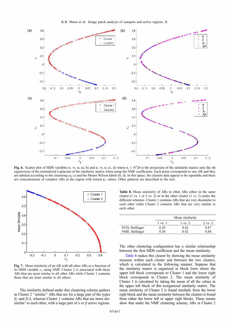
This relationship between AR complexity and clusteringassignment is further noticeable in Figure 8 which gives a his-togram of the Mount Wilson classes divided by clusteringassignment. This figure shows clear patterns between theclusterings and Mount Wilson type distribution, where theclustering separates somewhat the complex sunspots fromthe simple sunspots. This suggests that these configurationsare clustering based on some measure of AR complexity.
The Hellinger-based clusterings are correlated with sunspotsize for some of the Mount Wilson classes, see Table 9. Basedon the mean and median number of pixels, the Hellinger dis-tance on the NMF coefficients tends to gather in Cluster 2the smallest AR from classes a, b, and bc. Similarly, the Hel-linger distance on the SVD coefficients separates the b and bcAR by size with Cluster 1 containing the largest and Cluster 2containing the smallest AR.
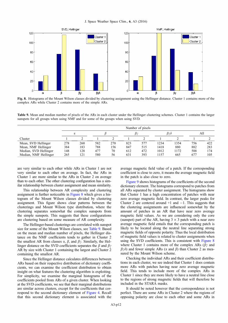
Since the Hellinger distance calculates differences betweenARs based on their respective distribution of dictionary coeffi-cients, we can examine the coefficient distribution to obtaininsight on what features the clustering algorithm is exploiting.For simplicity, we examine the marginal histograms of thecoefficients pooled from ARs of a given cluster. When lookingat the SVD coefficients, we see that their marginal distributionsare similar across clusters, except for the coefficients that cor-respond to the second dictionary element of Figure 4. Recallthat this second dictionary element is associated with the
average magnetic field value of a patch. If the correspondingcoefficient is close to zero, it means the average magnetic fieldin the patch is also close to zero.
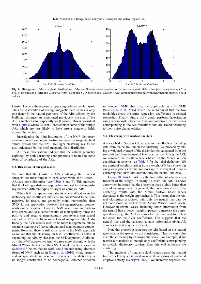
Figure 9 shows histograms of the coefficients of the seconddictionary element. The histograms correspond to patches fromall ARs separated by cluster assignment. The histograms showthat Cluster 1 has a high concentration of patches with nearzero average magnetic field. In contrast, the larger peaks forCluster 2 are centered around +1 and �1. This suggests thatthe clustering assignments are influenced somewhat by theamount of patches in an AR that have near zero averagemagnetic field values. As we are considering only the core(sunspot) part of the AR, having 3 · 3 patch with a near zeroaverage magnetic field entails that the corresponding patch islikely to be located along the neutral line separating strongmagnetic fields of opposite polarity. Thus the local distributionof magnetic field values is related to cluster assignments whenusing the SVD coefficients. This is consistent with Figure 8where Cluster 1 contains more of the complex ARs (bc andbcd) and fewer simple ARs (a and b) than Cluster 2 as mea-sured by the Mount Wilson scheme.
Checking the individual ARs and their coefficient distribu-tions in each cluster, we see indeed that Cluster 1 does containmore ARs with patches having near zero average magneticfield. This tends to include more of the complex ARs inCluster 1 since they are more likely to have a neutral line closeto the regions of strong magnetic fields that will therefore beincluded in the STARA masks.
It should be noted however that the correspondence is notperfect. There are some ARs in Cluster 2 where the regions ofopposing polarity are close to each other and some ARs in
Fig. 8. Histograms of the Mount Wilson classes divided by clustering assignment using the Hellinger distance. Cluster 1 contains more of thecomplex ARs while Cluster 2 contains more of the simple ARs.
Table 9. Mean and median number of pixels of the ARs in each cluster under the Hellinger clustering schemes. Cluster 1 contains the largersunspots for all groups when using NMF and for some of the groups when using SVD.
Number of pixels
a b bc bcd All
Cluster 1 2 1 2 1 2 1 2 1 2Mean, SVD Hellinger 278 260 582 270 823 577 1234 1354 756 422Mean, NMF Hellinger 384 183 788 156 847 515 1418 880 882 283Median, SVD Hellinger 148 128 477 70 612 472 1012 1172 588 174Median, NMF Hellinger 265 121 580 56 631 393 1157 665 677 105
J. Space Weather Space Clim., 6, A3 (2016)
A3-p12
Cluster 1 where the regions of opposing polarity are far apart.Thus the distribution of average magnetic field values is onlyone factor in the natural geometry of the ARs defined by theHellinger distance. As mentioned previously, the size of theAR is another factor, especially for b groups. This is consistentwith Figure 8 where Cluster 1 does contain some of the simpleARs which are less likely to have strong magnetic fieldsaround the neutral line.
Investigating the joint histograms of the NMF dictionaryelements corresponding to positive and negative magnetic fieldvalues reveals that the NMF Hellinger clustering results arealso influenced by the local magnetic field distribution.
All these observations indicate that the natural geometryexploited by both clustering configurations is related to someform of complexity of the ARs.
5.2. Discussion of sunspot results
We note that the Cluster 2 ARs containing the smallestsunspots are most similar to each other while the Cluster 1ARs are more dissimilar (see Tables 8 and 9). This indicatesthat the Hellinger distance approaches are best for distinguish-ing between different types of larger or complex ARs.
When NMF is applied on datasets where all values in thedictionary and coefficient matrices are constrained to be non-negative, its results are generally more interpretable thanSVD. In our application however, the magnetogram compo-nents can be negative. Hence the NMF results are not particu-larly sparse and lose some benefits of nonnegativity since thepositive and negative magnetogram components can canceleach other. This results in some loss of interpretability. Addi-tionally, the SVD results seem to be more interpretable due toseparate treatment of the continuum and magnetogram compo-nents. However, there is still some value in the NMF approachas we see that the clustering on NMF coefficients is better atseparating the ARs by size than the SVD approach. Addition-ally, the NMF approaches tend to agree more strongly with theMount Wilson labels than their SVD counterparts as is seen inSection 5.3 below. Future work could include using alternateforms of NMF such as in Ding et al. (2010) where sparsityand interpretability is preserved even when the dictionary isno longer constrained to be nonnegative. Another variation
in coupled NMF that may be applicable is soft NMF(Seichepine et al. 2014) where the requirement that the twomodalities share the same regression coefficients is relaxedsomewhat. Finally, future work could perform factorizationusing a composite objective function comprised of two termscorresponding to the two modalities that are scaled accordingto their noise characteristics.
5.3. Clustering with neutral line data
As described in Section 4.3, we analyze the effects of includingdata from the neutral line in the clustering. We proceed by tak-ing a weighted average of the dissimilarities calculated from thesunspots and from the neutral line data matrices. Using the ARI,we compare the results to labels based on the Mount Wilsonclassification scheme, see Table 7 for the label definition. Weuse a grid of weights, starting from a weight of 0 for a clusteringusing only patches within sunspots up to a weight of 1 for aclustering that takes into account only the neutral line data.
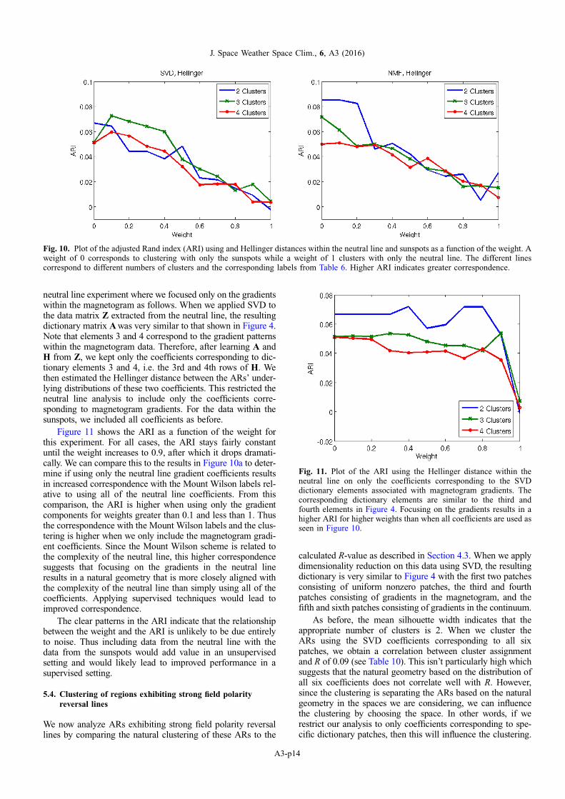
Figure 10 plots the ARI for the four different schemes as afunction of the weight. In nearly all cases, the ARI is abovezero which indicates that the clustering does slightly better thana random assignment. In general, the correspondence of theclustering results with the Mount Wilson based labelsdecreases as the weight approaches 1. This means that the nat-ural clusterings associated with only the neutral line data donot correspond as well with the Mount Wilson based labels.However in several cases, including some information fromthe neutral line at lower weights appears to increase the corre-spondence, e.g., the ARI increases for the three and four clus-ter cases for the SVD coefficients. This suggests that theneutral line and the sunspots contain information about ARcomplexity that may be different.
Note that clustering separates the ARs based on the naturalgeometry in the spaces we are considering. Thus we can influ-ence the clustering by choosing the space. For example, if werestrict our analysis to include only coefficients correspondingto specific dictionary patches, then this will influence theclustering.
The gradients of magnetic field values across the neutralline are a key quantity used in several indicators of potentialeruptive activity (Schrijver 2007). We therefore repeated the
Fig. 9. Histograms of the marginal distributions of the coefficients corresponding to the mean magnetic field value (dictionary element 2 inFig. 3) for Cluster 1 (left) and Cluster 2 (right) using the SVD coefficients. Cluster 1 ARs contain more patches with near neutral magnetic fieldvalues.
K.R. Moon et al.: Image patch analysis of sunspots and active regions. II.
A3-p13
neutral line experiment where we focused only on the gradientswithin the magnetogram as follows. When we applied SVD tothe data matrix Z extracted from the neutral line, the resultingdictionary matrix A was very similar to that shown in Figure 4.Note that elements 3 and 4 correspond to the gradient patternswithin the magnetogram data. Therefore, after learning A andH from Z, we kept only the coefficients corresponding to dic-tionary elements 3 and 4, i.e. the 3rd and 4th rows of H. Wethen estimated the Hellinger distance between the ARs’ under-lying distributions of these two coefficients. This restricted theneutral line analysis to include only the coefficients corre-sponding to magnetogram gradients. For the data within thesunspots, we included all coefficients as before.
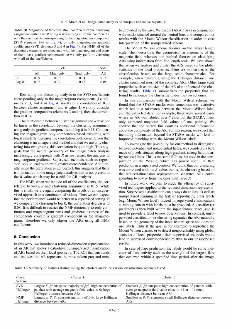
Figure 11 shows the ARI as a function of the weight forthis experiment. For all cases, the ARI stays fairly constantuntil the weight increases to 0.9, after which it drops dramati-cally. We can compare this to the results in Figure 10a to deter-mine if using only the neutral line gradient coefficients resultsin increased correspondence with the Mount Wilson labels rel-ative to using all of the neutral line coefficients. From thiscomparison, the ARI is higher when using only the gradientcomponents for weights greater than 0.1 and less than 1. Thusthe correspondence with the Mount Wilson labels and the clus-tering is higher when we only include the magnetogram gradi-ent coefficients. Since the Mount Wilson scheme is related tothe complexity of the neutral line, this higher correspondencesuggests that focusing on the gradients in the neutral lineresults in a natural geometry that is more closely aligned withthe complexity of the neutral line than simply using all of thecoefficients. Applying supervised techniques would lead toimproved correspondence.
The clear patterns in the ARI indicate that the relationshipbetween the weight and the ARI is unlikely to be due entirelyto noise. Thus including data from the neutral line with thedata from the sunspots would add value in an unsupervisedsetting and would likely lead to improved performance in asupervised setting.
5.4. Clustering of regions exhibiting strong field polarityreversal lines
We now analyze ARs exhibiting strong field polarity reversallines by comparing the natural clustering of these ARs to the
calculated R-value as described in Section 4.3. When we applydimensionality reduction on this data using SVD, the resultingdictionary is very similar to Figure 4 with the first two patchesconsisting of uniform nonzero patches, the third and fourthpatches consisting of gradients in the magnetogram, and thefifth and sixth patches consisting of gradients in the continuum.
As before, the mean silhouette width indicates that theappropriate number of clusters is 2. When we cluster theARs using the SVD coefficients corresponding to all sixpatches, we obtain a correlation between cluster assignmentand R of 0.09 (see Table 10). This isn’t particularly high whichsuggests that the natural geometry based on the distribution ofall six coefficients does not correlate well with R. However,since the clustering is separating the ARs based on the naturalgeometry in the spaces we are considering, we can influencethe clustering by choosing the space. In other words, if werestrict our analysis to only coefficients corresponding to spe-cific dictionary patches, then this will influence the clustering.
Fig. 11. Plot of the ARI using the Hellinger distance within theneutral line on only the coefficients corresponding to the SVDdictionary elements associated with magnetogram gradients. Thecorresponding dictionary elements are similar to the third andfourth elements in Figure 4. Focusing on the gradients results in ahigher ARI for higher weights than when all coefficients are used asseen in Figure 10.
Fig. 10. Plot of the adjusted Rand index (ARI) using and Hellinger distances within the neutral line and sunspots as a function of the weight. Aweight of 0 corresponds to clustering with only the sunspots while a weight of 1 clusters with only the neutral line. The different linescorrespond to different numbers of clusters and the corresponding labels from Table 6. Higher ARI indicates greater correspondence.
J. Space Weather Space Clim., 6, A3 (2016)
A3-p14
Restricting the clustering analysis to the SVD coefficientscorresponding only to the magnetogram components (i.e. ele-ments 2, 3, and 4 in Fig. 4) results in a correlation of 0.30between cluster assignment and R-value. If we only considerthe gradient components (elements 3 and 4), then the correla-tion is 0.34.
The relationship between cluster assignment and R may notbe linear as the correlation between the clustering assignmentusing only the gradient components and log R is 0.45. Compar-ing the magnetogram only components-based clustering withlog R similarly increases the correlation coefficient. Given thatclustering is an unsupervised method and that we are only clus-tering into two groups, this correlation is quite high. This sug-gests that the natural geometry of the image patch analysisincreasingly corresponds with R as we restrict the analysis tomagnetogram gradients. Supervised methods, such as regres-sion, should lead to an even greater correspondence. Addition-ally, since the correlation is not perfect, this suggests that thereis information in the image patch analysis that is not present inthe R-value which may be useful for AR analysis.
For NMF, when we include all of the coefficients, the cor-relation between R and clustering assignment is 0.15. Whilethis is small, we are again comparing the labels of an unsuper-vised approach to a continuum of values. Thus we can expectthat the performance would be better in a supervised setting. Ifwe compare the clusering to log R, the correlation decreases to0.08. It is difficult to restrict the NMF dictionary to only con-tinuum and magnetogram parts and gradients as most of thecomponents contain a gradient component in the magneto-gram. Therefore we only cluster the ARs using all NMFcoefficients.
6. Conclusion
In this work, we introduce a reduced-dimension representationof an AR that allows a data-driven unsupervised classificationof ARs based on their local geometry. The ROI that surroundsand includes the AR represents its most salient part and must
be provided by the user. We used STARA masks in conjunctionwith masks situated around the neutral line, and compared ourresults with the Mount Wilson classification in order to easeinterpretation of the unsupervised scheme.
The Mount Wilson scheme focuses on the largest lengthscale when describing the geometrical arrangements of themagnetic field, whereas our method focuses on classifyingARs using information from fine length scale. We have shownthat when we analyze and cluster the ARs based on the globalstatistics of the local properties, there are similarities to theclassification based on the large scale characteristics. Forexample, when clustering using the Hellinger distance, onecluster contained most of the complex ARs. Other large scaleproperties such as the size of the AR also influenced the clus-tering results. Table 11 summarizes the properties that arefound to influence the clustering under the two schemes.
In this comparison with the Mount Wilson scheme, wefound that the STARA masks were sometimes too restrictivewhich led to a mismatch between the Mount Wilson labeland the extracted data. For example, there were several caseswhere an AR was labeled as a b class but the STARA maskonly extracted magnetic field values of one polarity. Weshowed that the neutral line contains additional informationabout the complexity of the AR. For this reason, we expect thatincluding information beyond the STARA masks will lead toimproved matching with the Mount Wilson labels.
To investigate the possibility for our method to distinguishbetween potential and nonpotential fields, we considered a ROImade of pixels situated along high-gradient, strong field polar-ity reversal lines. This is the same ROI as that used in the com-putation of the R-value, which has proved useful in flareprediction in a supervised context. We found that our clusteringwas correlated with the R-value, that is, the clustering based onthe reduced-dimension representation separates ARs corre-sponding to low R from the ones with large R.
In future work, we plan to study the efficiency of super-vised techniques applied to the reduced dimension representa-tion. Supervised classification can always do at least as well asunsupervised learning in the task of reproducing class labels(e.g. Mount Wilson label). Indeed, in supervised classification,a training dataset with labels must be provided. A classifier (orpredictor) is then built within the input feature space, and isused to provide a label to new observations. In contrast, unsu-pervised classification or clustering separates the ARs naturallybased on the geometry of the input feature space and does notuse labels. Thus if the goal is for example to reproduce theMount Wilson classes, or to detect nonpotentiality using globalstatistics of local properties, then supervised methods wouldlead to increased correspondence relative to our unsupervisedresults.
In case of flare prediction, the labels would be some indi-cator of flare activity such as the strength of the largest flarethat occurred within a specified time period after the image
Table 10. Magnitude of the correlation coefficient of the clusteringassignment with either R or log R when using all of the coefficients,only the coefficients corresponding to the magnetogram component(SVD elements 2–4 in Fig. 4), or only magnetogram gradientcoefficients (SVD elements 3 and 4 in Fig. 4). For NMF, all of thedictionary elements are associated with the magnetogram and manyof them have gradient components so we only perform clusteringwith all of the coefficients.
SVD NMF
All Mag. only Grad. only AllR 0.09 0.30 0.34 0.15log R 0.02 0.37 0.45 0.08
Table 11. Summary of features distinguishing the clusters under the various classification schemes tested.
Class.Scheme
Cluster 1 Cluster 2
SVDHellinger
Largest b, bc sunspots; majority of bcd; high concentration ofpatches with average magnetic field value ’ 0; largeHellinger distance between ARs
Smallest b, bc sunspots; high concentration of patches withaverage magnetic field value close to +1 or �1; smallHellinger distance between ARs
NMFHellinger
Largest a, b, bc sunspots;majority of bcd; large Hellingerdistance between ARs
Smallest a, b, bc sunspots; small Hellinger distance betweenARs
K.R. Moon et al.: Image patch analysis of sunspots and active regions. II.
A3-p15
was taken. Supervised techniques such as classification orregression could be applied depending on the nature of thelabel (i.e. categorical vs. continuum).
A good way of assessing how well a given feature space cando in a supervised setting is to estimate the Bayes error. TheBayes error gives the minimum average probability of error thatany classifier can achieve on the given data and can be esti-mated in the two class setting by estimating upper and lowerbounds such as the Chernoff bound using a divergence-basedestimator as in Moon & Hero III (2014b). These bounds canbe estimated using various schemes and combinations of data(inside sunspots, along the neutral line, etc.) to determine whichscheme is best at reproducing the desired labels (e.g., theMount Wilson labels). This can also be done in combinationwith physical parameters of the ARs such those used in Bobra& Couvidat (2015) (e.g. the total unsigned flux, the total area,the sum of flux near the polarity-inversion line, etc.).
These methods of comparing AR images can also beadapted to a time series of image pairs. For example, imagepairs from a given point in time may be compared to the imagepairs from an earlier period to measure how much the ARshave changed. The evolution of an AR may also be studiedby defining class labels based on the results from one of theclustering schemes in this paper. From the clustering results,a classifier may be trained that is then used to assign an ARto one of these clusters at each time step. The evolution ofthe AR’s cluster assignment can then be examined.
Acknowledgements. This work was partially supported by the USNational Science Foundation (NSF) under Grant CCF-1217880and a NSF Graduate Research Fellowship to KM under Grant No.F031543. VD acknowledges support from the Belgian Federal Sci-ence Policy Office through the ESA-PRODEX program, Grant No.4000103240, while RDV acknowledges support from the BRAIN.beprogram of the Belgian Federal Science Policy Office, Contract No.BR/121/PI/PREDISOL. We thank Dr. Laura Balzano at the Univer-sity of Michigan, as well as Dr. Laure Lefèvre, Dr. Raphael Attie,and Ms. Marie Dominique at the Royal Observatory of Belgiumfor their feedback on the manuscript. The authors gratefullyacknowledge Dr. Paul Shearer’s help in implementing the modifiedNMF algorithm. The editor thanks two anonymous referees for theirassistance in evaluating this paper.
References
Ahmed, O.W., R. Qahwaji, T. Colak, P.A. Higgins, P.T. Gallagher,and D.S. Bloomfield. Solar flare prediction using advancedfeature extraction, machine learning, and feature selection. Sol.Phys., 283, 157–175, 2013, DOI: 10.1007/s11207-011-9896-1.
Barnes, G., K.D. Leka, E.A. Schumer, and D.J. Della-Rose.Probabilistic forecasting of solar flares from vector magnetogramdata. Space Weather, 5, S09002, 2007,DOI: 10.1029/2007SW000317.
Bazot, C., N. Dobigeon, J.-Y. Tourneret, A. Zaas, G. Ginsburg, andA.O. Hero III. Unsupervised Bayesian linear unmixing of geneexpression microarrays. BMC Bioinf., 14 (1), 99, 2013,DOI: 10.1186/1471-2105-14-99.
Bhattacharyya, A. On a measure of divergence between twomultinomial populations. Sankhya, 7 (4), 401–406, 1946.
Bioucas-Dias, J.M., A. Plaza, N. Dobigeon, M. Parente, Q. Du, P.Gader, and J. Chanussot. Hyperspectral unmixing overview:geometrical, statistical, and sparse regression-based approaches.IEEE J. Sel. Topics Appl. Earth Observations Remote Sensing,5 (2), 354–379, 2012.
Bobra, M.G., and S. Couvidat. Solar flare prediction using SDO/HMI vector magnetic field data with a machine-learning
algorithm. Astrophys. J., 798, 135, 2015,DOI: 10.1088/0004-637X/798/2/135.
Colak, T., and R. Qahwaji. Automated McIntosh-based classifica-tion of sunspot groups using MDI images. Sol. Phys., 248,277–296, 2008, DOI: 10.1007/s11207-007-9094-3.
Colak, T., and R. Qahwaji. Automated solar activity prediction:a hybrid computer platform using machine learning and solarimaging for automated prediction of solar flares. Space Weather,7, S06001, 2009, DOI: 10.1029/2008SW000401.
Comon, P., and C. Jutten. Handbook of Blind Source Separation:Independent Component Analysis and Blind Deconvolution.Academic Press, Oxford, 2010.
Csiszar, I. Information-type measures of difference of probabilitydistributions and indirect observations. Studia Sci. Math.Hungar., 2, 299–318, 1967.
DeForest, C. On re-sampling of solar images. Sol. Phys., 219 (1),3–23, 2004.
Ding, C., T. Li, and M.I. Jordan. Convex and semi-nonnegativematrix factorizations. IEEE Trans. Pattern Anal. Mach. Intell.,32 (1), 45–55, 2010.
Dudok de Wit, T., S. Moussaoui, C. Guennou, F. Auchère, G.Cessateur, M. Kretzschmar, L.A. Vieira, and F.F. Goryaev.Coronal temperature maps from solar EUV images: a blindsource separation approach. Sol. Phys., 283, 31–47, 2013,DOI: 10.1007/s11207-012-0142-2.
Edelman, A., T.A. Arias, and S.T. Smith. The geometry ofalgorithms with orthogonality constraints. SIAM J. Matrix Anal.Appl., 20 (2), 303–353, 1998.
Falconer, D.A., R.L. Moore, and G.A. Gary. Magnetogram measuresof total nonpotentiality for prediction of solar coronal massejections from active regions of any degree of magneticcomplexity. Astrophys. J., 689, 1433–1442, 2008,DOI: 10.1086/591045.
Galluccio, L., O. Michel, P. Comon, M. Kliger, and A.O. Hero III.Clustering with a new distance measure based on a dual-rootedtree. Inform. Sciences, 251, 96–113, 2013.
Georgoulis, M.K., and D.M. Rust. Quantitative forecasting of majorsolar flares. Astrophys. J. Lett., 661, L109–L112, 2007,DOI: 10.1086/518718.
Guo, J., H. Zhang, O.V. Chumak, and Y. Liu. A quantitative study onmagnetic configuration for active regions. Sol. Phys., 237, 25–43,2006, DOI: 10.1007/s11207-006-2081-2.
Györi, L., T. Baranyi, and A. Ludmány. Photospheric data programsat the Debrecen observatory. Proc. Int. Astron. Union, 6 (S273),403–407, 2010.
Hale, G.E., F. Ellerman, S.B. Nicholson, and A.H. Joy. Themagnetic polarity of sun-spots. Astrophys. J., 49, 153, 1919,DOI: 10.1086/142452.
Hellinger, E. Neue Begründung der Theorie quadratischer Formenvon unendlichvielen Veränderlichen. Journal für die reine undangewandte Mathematik, 136, 210–271, 1909.
Higgins, P.A., P.T. Gallagher, R. McAteer, and D.S. Bloomfield.Solar magnetic feature detection and tracking for space weathermonitoring. Adv. Space Res., 47 (12), 2105–2117, 2011.
Huang, X., D. Yu, Q. Hu, H. Wang, and Y. Cui. Short-term solarflare prediction using predictor teams. Sol. Phys., 263, 175–184,2010, DOI: 10.1007/s11207-010-9542-3.
Jolliffe, I.T. Principal Component Analysis, 2nd ed., Springer-Verlag New York, Inc., New York, 2002.
Kruskal, J.B., and M. Wish. Multidimensional Scaling, vol. 11,Sage, New York, 1978.
Kullback, S., and R.A. Leibler. On information and sufficiency. Ann.Math. Stat., 22, 79–86, 1951.
Künzel, H. Die Flare-Häufigkeit in Fleckengruppen unterschiedli-cher Klasse und magnetischer Struktur. Astron. Nachr., 285,271–271, 1960.
Langville, A.N., C.D. Meyer, R. Albright, J. Cox, and D. Duling.Initializations for the nonnegative matrix factorization, inProceedings of the Twelfth ACM SIGKDD International
J. Space Weather Space Clim., 6, A3 (2016)
A3-p16
Conference on Knowledge Discovery and Data Mining,Philadelphia, USA, Citeseer, 2006.
Lee, D.D., and H.S. Seung. Algorithms for non-negative matrixfactorization, in Advances in Neural Information ProcessingSystems (NIPS), 556–562, 2001.
Lee, K., Y.-J. Moon, J.-Y. Lee, K.-S. Lee, and H. Na. Solar flareoccurrence rate and probability in terms of the sunspot classi-fication supplemented with sunspot area and its changes. Sol.Phys., 281, 639–650, 2012, DOI: 10.1007/s11207-012-0091-9.
Leka, K.D., and G. Barnes. Photospheric magnetic field propertiesof flaring vs. flare-quiet active regions III: discriminant analysisof a statistically significant database. In American AstronomicalSociety Meeting Abstracts #204, vol. 36 of Bulletin of theAmerican Astronomical Society, 715, 2004.
Lin, C.-J. Projected gradient methods for nonnegative matrixfactorization. Neural Comput., 19 (10), 2756–2779, 2007.
Mayfield, E.B., and J.K. Lawrence. The correlation of solar flareproduction with magnetic energy in active regions. Sol. Phys., 96,293–305, 1985, DOI: 10.1007/BF00149685.
Mittelman, R., N. Dobigeon, and A. Hero. Hyperspectral imageunmixing using a multiresolution sticky HDP. IEEE Trans. SignalProcess., 60 (4), 1656–1671, 2012,DOI: 10.1109/TSP.2011.2180718.
Moon, K.R., and A.O. Hero III. Ensemble estimation of multivariatef-divergence, in Information Theory (ISIT), 2014 IEEE Interna-tional Symposium on, Honolulu, USA, IEEE, 356–360, 2014a.
Moon, K.R., and A.O. Hero III. Multivariate f-divergence estima-tion with confidence. Adv. Neural Inf. Process. Syst., 27,2420–2428, 2014b.
Moon, K.R., J.J. Li, V. Delouille, F. Watson, and A.O. Hero III.Image patch analysis and clustering of sunspots: a dimensionalityreduction approach, in IEEE International Conference on ImageProcessing (ICIP), Paris, France, IEEE, 1623–1627, 2014.
Moon, K.R., J.J. Li, V. Delouille, R. De Visscher, F. Watson, andA.O. Hero III. Image patch analysis of sunspots and activeregions. I. Intrinsic dimension and correlation analysis. J. SpaceWeather Space Clim., 2015.
Moon, T.K., and W.C. Stirling. Mathematical Methods and Algo-rithms for Signal Processing, Prentice Hall, New York, 2000.
Prim, R.C. Shortest connection networks and some generalizations.Bell Syst. Tech. J., 36 (6), 1389–1401, 1957.
Ramírez, I., and G. Sapiro. An MDL framework for sparse codingand dictionary learning. IEEE Trans. Signal Process., 60 (6),2913–2927, 2012.
Rand, W.M. Objective criteria for the evaluation of clusteringmethods. J. Amer. Statist. Assoc., 66 (336), 846–850, 1971.
Rousseeuw, P.J. Silhouettes: a graphical aid to the interpretation andvalidation of cluster analysis. J. Comput. Appl. Math., 20, 53–65,1987.
Sammis, I., F. Tang, and H. Zirin. The dependence of large flareoccurrence on the magnetic structure of sunspots. Astrophys. J.,540, 583–587, 2000, DOI: 10.1086/309303.
Scherrer, P.H., R.S. Bogart, R.I. Bush, J.T. Hoeksema, A.G.Kosovichev, et al. The solar oscillations investigation –Michelson Doppler imager. Sol. Phys., 162, 129–188, 1995,DOI: 10.1007/BF00733429.
Schrijver, C.J. A characteristic magnetic field pattern associatedwith all major solar flares and its use in flare forecasting.Astrophys. J. Lett., 655, L117–L120, 2007,DOI: 10.1086/511857.
Seichepine, N., S. Essid, C. Févotte, and O. Cappé. Soft nonnegativematrix co-factorization. IEEE Trans. Signal Process., 62 (22),5940–5949, 2014.
Sethian, J.A. A fast marching level set method for monotonicallyadvancing fronts. Proc. Nat. Acad. Sci., 93, 1591–1595, 1995.
Song, H., C. Tan, J. Jing, H. Wang, V. Yurchyshyn, and V.Abramenko. Statistical assessment of photospheric magneticfeatures in imminent solar flare predictions. Sol. Phys., 254,101–125, 2009, DOI: 10.1007/s11207-008-9288-3.
Stenning, D.C., T.C.M. Lee, D.A. van Dyk, V. Kashyap, J. Sandell,and C.A. Young. Morphological feature extraction for statisticallearning with applications to solar image data. Stat. Anal. DataMin., 6 (4), 329–345, 2013, DOI: 10.1002/sam.11200.
Stewart, G.W. Error and perturbation bounds for subspacesassociated with certain eigenvalue problems. SIAM Rev., 15 (4),727–764, 1973.
Warwick, C.S. Sunspot configurations and proton flares. Astrophys.J., 145, 215, 1966, DOI: 10.1086/148755.
Watson, F.T., L. Fletcher, and S. Marshall. Evolution of sunspotproperties during solar cycle 23. Astron. Astrophys., 533, A14,2011, DOI: 10.1051/0004-6361/201116655.
Yaghoobi, M., T. Blumensath, and M.E. Davies. Dictionary learningfor sparse approximations with the majorization method, IEEETrans. Signal Process., 57 (6), 2178–2191, 2009.
Yokoya, N., T. Yairi, and A. Iwasaki. Coupled nonnegative matrixfactorization unmixing for hyperspectral and multispectral datafusion. IEEE Trans. Geosci. Remote Sens., 50 (2), 528–537,2012.
Yu, D., X. Huang, H. Wang, Y. Cui, Q. Hu, and R. Zhou. Short-termsolar flare level prediction using a Bayesian network approach.Astrophys. J., 710, 869–877, 2010,DOI: 10.1088/0004-637X/710/1/869.
Cite this article as: Moon KR, Delouille V, Li JJ, De Visscher R, Watson F, et al. Image patch analysis of sunspots and active regions.II. Clustering via matrix factorization. J. Space Weather Space Clim., 6, A3, 2016, DOI: 10.1051/swsc/2015043.
K.R. Moon et al.: Image patch analysis of sunspots and active regions. II.
A3-p17
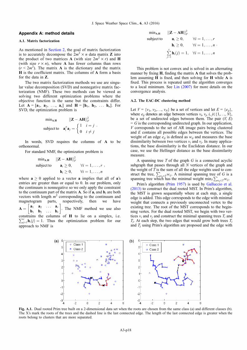
Appendix A: method details
A.1. Matrix factorization
As mentioned in Section 2, the goal of matrix factorizationis to accurately decompose the 2m2 · n data matrix Z intothe product of two matrices A (with size 2m2 · r) and H(with size r · n), where A has fewer columns than rows(r < 2m2). The matrix A is the dictionary and the matrixH is the coefficient matrix. The columns of A form a basisfor the data in Z.
The two matrix factorization methods we use are singu-lar value decomposition (SVD) and nonnegative matrix fac-torization (NMF). These two methods can be viewed assolving two different optimization problems where theobjective function is the same but the constraints differ.Let A = [a1, a2, . . ., ar] and H = [h1, h2, . . . hn]. ForSVD, the optimization problem is
minA;H jjZ� AHjj2F
subject to aTi aj ¼
1 i ¼ j
0 i 6¼ j
�:
In words, SVD requires the columns of A to beorthonormal.
For standard NMF, the optimization problem is
minA;H jjZ� AHjj2Fsubject to ai � 0; 8i ¼ 1; . . . ; r
hi � 0; 8i ¼ 1; . . . ; n
;
where a � 0 applied to a vector a implies that all of a’sentries are greater than or equal to 0. In our problem, onlythe continuum is nonnegative so we only apply the constraintto the continuum part of the matrix A. So if ai and bi are bothvectors with length m2 corresponding to the continuum andmagnetogram parts, respectively, then we have
A ¼ a1 a2 . . . ar
b1 b2 . . . br
� . The NMF method we use also
constrains the columns of H to lie on a simplex, i.e.Prj¼1hiðjÞ ¼ 1. Thus the optimization problem for our
approach to NMF is
minA;H jjZ� AHjj2Fsubject to ai � 0; 8i ¼ 1; . . . ; r
hi � 0; 8i ¼ 1; . . . ; nPrj¼1
hiðjÞ ¼ 1; 8i ¼ 1; . . . ; n
:
This problem is not convex and is solved in an alternatingmanner by fixing H, finding the matrix A that solves the prob-lem assuming H is fixed, and then solving for H while A isfixed. This process is repeated until the algorithm convergesto a local minimum. See Lin (2007) for more details on theconvergence analysis.
A.2. The EAC-DC clustering method
Let V = {v1, v2,. . ., vN} be a set of vertices and let E = {eij},where eij denotes an edge between vertices vi, vj, i, j2{1,. . ., N},be a set of undirected edges between them. The pair (V, E)= G is the corresponding undirected graph. In our application,V corresponds to the set of AR image pairs being clusteredand E contains all possible edges between the vertices. Theweight of an edge eij is defined as wij and measures the basedissimilarity between two vertices vi and vj. In many applica-tions, the base dissimilarity is the Euclidean distance. In ourcase, we use the Hellinger distance as the base dissimilaritymeasure.
A spanning tree T of the graph G is a connected acyclicsubgraph that passes through all N vertices of the graph andthe weight of T is the sum of all the edge weights used to con-struct the tree,
Peij2T wij. A minimal spanning tree of G is a
spanning tree which has the minimal weight minTP
eij2T wij.Prim’s algorithm (Prim 1957) is used by Galluccio et al.
(2013) to construct the dual rooted MST. In Prim’s algorithm,the MST is grown sequentially where at each step, a singleedge is added. This edge corresponds to the edge with minimalweight that connects a previously unconnected vertex to theexisting tree. The root of the MST corresponds to the begin-ning vertex. For the dual rooted MST, we begin with two ver-tices vi and vj and construct the minimal spanning trees Ti andTj. At each step, the two edges that would grow both trees Ti
and Tj using Prim’s algorithm are proposed and the edge with
Fig. A.1. Dual rooted Prim tree built on a 2-dimensional data set when the roots are chosen from the same class (a) and different classes (b).The X’s mark the roots of the trees and the dashed line is the last connected edge. The length of the last connected edge is greater when theroots belong to clusters that are more separated.
J. Space Weather Space Clim., 6, A3 (2016)
A3-p18
minimal weight is added. This continues until Ti and Tj con-nect. The weight of the final edge added in this algorithmdefines a new metric between the vertices vi and vj. This pro-cess is repeated for all pairs of vertices and this new metric isused as input to spectral clustering (Galluccio et al. 2013).
A primary advantage of this metric based on the hittingtime of the two MSTs is that it depends on the MST topologyof the data. Thus if two vertices belong to the same cluster,then the MST distance between them will be small since clus-ter points will be close together. This is the case even if the ver-tices are far away from each other (e.g. on opposite ends of thecluster). However, if the two vertices are in different clustersthat are well separated, then the MST distance between themwill be large. See Figure A.1 for an example. Thus this methodof clustering is very robust to the shape of the clusters.Galluccio et al. (2013) contains many more examples.
The MST-based metric can be computationally intensive tocompute as Prim’s algorithm must be run as many times asthere are pairs of vertices. To counter this, Galluccio et al.(2013) proposed the EAC-DC algorithm which uses the infor-mation from only a subset of the dual rooted MSTs. This isdone by calculating the dual rooted MSTs for a random pairof vertices. Three clusters are defined for each run: all verticesthat are connected to one of the roots in the MSTs form two ofthe clusters (one for each root) while all points that are not con-nected to either of the MSTs are assigned to a third ‘‘rejection’’cluster. A co-association measure for two vertices is thendefined as the number of times those vertices are containedin the same nonrejection cluster divided by the total numberof runs (dual rooted MSTs). This co-association measure formsa similarity measure to which spectral clustering is applied.
K.R. Moon et al.: Image patch analysis of sunspots and active regions. II.
A3-p19