18 T. FRÝZA, S. HANUS, IMAGE COMPRESSION ALGORITHMS OPTIMIZED FOR MATLAB

Image Compression Algorithms Optimized for MATLAB

Tomáš FRÝZA, Stanislav HANUS

Dept. of Radio Electronics, Brno University of Technology, Purkyňova 118, 612 00 Brno, Czech Republic

fryza@feec.vutbr.cz, hanus@feec.vutbr.cz

Abstract. This paper describes implementation of the Discrete Cosine Transform (DCT) algorithm to MATLAB. This approach is used in JPEG or MPEG standards for instance. The substance of these specifications is to remove the considerable correlation between adjacent picture elements.

The objective of this paper is not to improve the DCT algorithm it self, but to re-write it to the preferable version for MATLAB thus allows the enumeration with insignificant delay. The method proposed in this paper allows image compression calculation almost two hundred times faster compared with the DCT definition.

Keywords MATLAB, algorithms, image compression, 2D DCT, NRMSE, calculation time.

1. Introduction The typical still images contain areas where

neighboring pixels have almost the same values therefore the spatial redundancy is considerable. To remove the redundancy, different methods (for lossy and lossless com-pression) have been developed.

One of the lossy methods is known as JPEG, the Joint Photographic Experts Group. Officially, JPEG corresponds to the ISI/IEC international standard 10928-1 and has been established by members from the International Telecom-munication Union (ITU) and the International Organization for Standardization (ISO).

In this contribution we attempt to optimize JPEG arithmetic operations for MATLAB. To examine computa-tional requirements of the proposed algorithm, we used seven test images with different dimensions.

2. JPEG Standard Based Image Compression In technique used in JPEG, the source image is di-

vided in 8×8 blocks and each block is transformed using the DCT. Each of the 64 DCT coefficients is achieved via

quantization followed by variable length coding.

By Wallace [1] the 2D fDCT (Forward Two-Dimen-sional Discrete Cosine Transform) is defined in the fol-lowing way:

∑∑= =

⋅⋅⋅⋅

=7

0

7

0,,,, 4 x yvyuxyx

vuvu DDpCCP (1)

where Pu,v is the 2D DCT coefficient, u,v=0,…,7, px,y is the intensity of picture element and constants C0=2-½ and Ck=1 for k=1,…,7. We construct a DCT transform base as follows:

( )16

12cos,πbaD ba

+= (2)

where parameters { }yxa , ∈ and b . { }vu, ∈

In a similar way we define the Inverse Two-Dimen-sional Discrete Cosine Transform (2D iDCT) of the form:

∑∑= =

⋅⋅⋅⋅

=7

0

7

0,,,, 4u vvyuxyx

vuyx DDPCCp . (3)

It is well-known rule to use as few cycles as possible in environment of MATLAB. Consequently we can not program (1-3) by series of two nested loops for one DCT coefficient, like we can probably do in the language C. In the next text we present source codes suitable for image compression in MATLAB.

2.1 2D DCT MATLAB Implementation The essence of the image coding implementation con-

sists in a conversion to the domain convenient for MAT-LAB, i.e. matrix operations [2]. Both of sums from (1, 3) can be overwritten to the scalar or matrix multiplication [2, 3]. Next paragraphs show source code of the encoder main function when test image is divided into 8×8 blocks and each block is multiplied by DCT base mUX, mYV defined in (2) and by scaling matrix mNORM which contains constants Ck. Subsequently, the DCT coefficients are quantized by a quantize matrix Qtab and save to a logical file fout via function store. for i = 0 : (nbx – 1) / 8, for j = 0 : (nby – 1) / 8, block = img (i*8+1 : (i+1)*8, j*8+1 : (j+1)*8) - 128 ;

RADIOENGINEERING, VOL. 12, NO. 4, DECEMBER 2003 19

coeff = mNORM .* (mUX * block * mYV) ; 50_100

QtabJPEG scalQtab new ⋅ + = (4) coeff = round (coeff ./ Qtab) ;

store (coeff, fout) ; end end where scal=5000/qf for qf <50, scal=200-2·qf for qf ≥50,

quality factor { }100,1 ∈qf and represents rounding

down. ⋅

All used constants are represented by the global variables defined in function initCts. Variable QtabJPEG specifies the quantization step size for each of the 64 DCT coefficients and it is the original quantize matrix for the luminance signals in JPEG standard [5].

function [Qtab] = QuantizeTab(qf) if (qf < 50)

function initCts scal = 5000 / qf ;

else end

scal = 200 – qf * 2 ; global mUX, mYV, mNORM, QtabJPEG, zig mUX = cos ([0:7]’ * (2*[0:7]+1) * pi/16) ;

Qtab_new = floor (((QtabJPEG .* scal) + 50) mYV = cos ((2*[0:7]’+1) * [0:7] * pi/16) ; ./ 100) ; mNORM = [1/2 ones(1,7) / sqrt(2); idz = find (Qtab_new <= 0) ; ones(7,1) / sqrt(2) ones(7,7)] / 4 ; Qtab_new (idz) = zeros (size(idz)) ; idz = find (Qtab_new > 255) ; QtabJPEG = [16 11 10 16 24 40 51 61; Qtab_new (idz) = 255*ones (size(idz)) ; 12 12 14 19 26 58 60 55; Qtab = Qtab_new ; 14 13 16 24 40 57 69 56;

14 17 22 29 51 87 80 62; 18 22 37 56 68 109 103 77; The DCT based compression system is limited by a

block based segmentation of the source image. The higher compress ratio the higher is image degradation.

24 35 55 64 81 104 113 92; 49 64 78 87 103 121 120 101; 72 92 95 98 112 100 103 99]; Each coefficient is coded by variable length coding

into the form of [number of zeros before non-null coeffi-cient, value of non-null coefficient] and stored to a file.

zig = [ 1 9 2 3 10 17 25 18 ... 11 4 5 12 19 26 33 41 ... 34 27 20 13 6 7 14 21 ... 28 35 42 49 57 50 43 36 ...

29 22 15 8 16 23 30 37 ... function store(coeff, fout) 44 51 58 59 52 45 38 31 ... 24 32 39 46 53 60 61 54 ... [Qtab, zig] = initCts ; 47 40 48 55 62 63 56 64] ; coeff_vector = coeff(:) ; vector = coeff_vector (zig) ; Last variable is a vector named zig with a size of

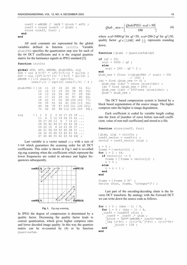
1×64 which guarantees the scanning order for all DCT coefficients. This order is shown in Fig.1 and is so-called zig-zag scanning when the coefficients which represent the lower frequencies are coded in advance and higher fre-quencies subsequently.

n = 0 ; frafor j = 2 : 64,

me = [vector(1)] ;

if vector(j) ~= 0 frame = [frame n vectro(j)] ; n = 0 ; else

coeff(8,1)

coeff(1,1) coeff(1,8)

coeff(8,8)

n = n + 1 ; end end frame = [frame 0 0]’ ; fwrite (fout, frame, ‘integer*1’) ;

Last part of the encoding/decoding chain is the In-verse DCT transform. By analogy with the Forward DCT we can write down the source code as follows. for = 0 : (nbx – 1) / 8, i for j = 0 : (nby – 1) / 8, Fig. 1. Zig-zag scanning.

_coeff = loadDCT (fin) ; In JPEG the degree of compression is determined by a quality factor. Decreasing the quality factor leads to coarser quantization, which gives higher compress ratio and lower decoded image quality. In this way the quantize matrix can be re-counted by (4) or by function QuantizeTab.

_coeff = _coeff .* Qtab ; _block = (mYV*(mNORM.*_coeff)*mUX) ; _img (i*8+1 : (i+1)*8, j*8+1 : (j+1)*8)=

_block + 128 ; end end

20 T. FRÝZA, S. HANUS, IMAGE COMPRESSION ALGORITHMS OPTIMIZED FOR MATLAB

2.2 Compression Quality Appreciation The fundamental aspect in testing image compression

methods is a final quality examination as well. We used the Normalized Root Mean Square Error (NRMSE) defined by (5).

( )

( )∑ ∑

∑ ∑−

=

−

=

−

=

−

=

−=

1

0

1

0

2,

1

0

1

0

2,,

ˆ

nbx

i

nby

jji

nbx

i

nby

jjiji

p

ppNRMSE (5)

where pi,j is the intensity of picture element and p^i,j is the

intensity of picture element of the reconstructed image when MATLAB source code is suggested below. NUM = img - _img ; NUM = NUM .^ 2 ; num = sum (NUM(:)) ; NRMSE = sqrt (num / sumsqr (img)) ;

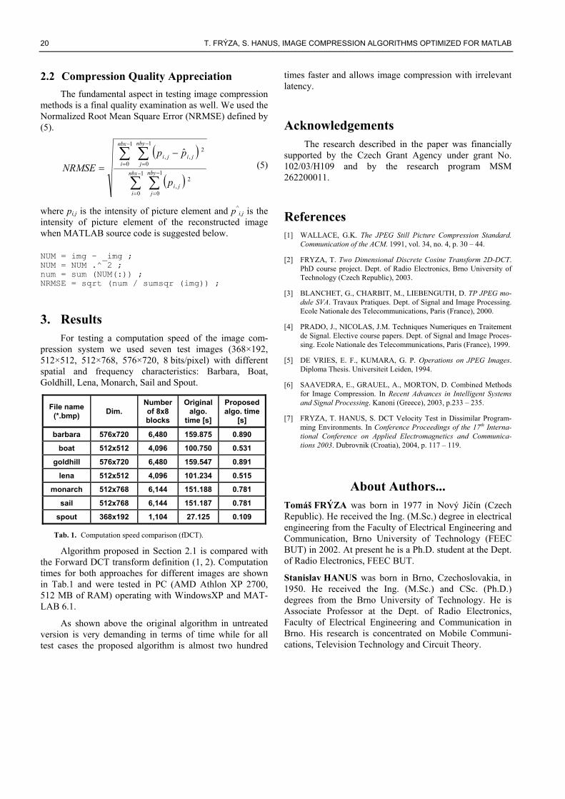
3. Results For testing a computation speed of the image com-

pression system we used seven test images (368×192, 512×512, 512×768, 576×720, 8 bits/pixel) with different spatial and frequency characteristics: Barbara, Boat, Goldhill, Lena, Monarch, Sail and Spout.

File name (*.bmp) Dim.

Number of 8x8 blocks

Original algo.

time [s]

Proposed algo. time

[s]

barbara 576x720 6,480 159.875 0.890

boat 512x512 4,096 100.750 0.531

goldhill 576x720 6,480 159.547 0.891

lena 512x512 4,096 101.234 0.515

monarch 512x768 6,144 151.188 0.781

sail 512x768 6,144 151.187 0.781

spout 368x192 1,104 27.125 0.109

Tab. 1. Computation speed comparison (fDCT).

Algorithm proposed in Section 2.1 is compared with the Forward DCT transform definition (1, 2). Computation times for both approaches for different images are shown in Tab.1 and were tested in PC (AMD Athlon XP 2700, 512 MB of RAM) operating with WindowsXP and MAT-LAB 6.1.

As shown above the original algorithm in untreated version is very demanding in terms of time while for all test cases the proposed algorithm is almost two hundred

times faster and allows image compression with irrelevant latency.

Acknowledgements The research described in the paper was financially

supported by the Czech Grant Agency under grant No. 102/03/H109 and by the research program MSM 262200011.

References [1] WALLACE, G.K. The JPEG Still Picture Compression Standard.

Communication of the ACM. 1991, vol. 34, no. 4, p. 30 – 44.

[2] FRYZA, T. Two Dimensional Discrete Cosine Transform 2D-DCT. PhD course project. Dept. of Radio Electronics, Brno University of Technology (Czech Republic), 2003.

[3] BLANCHET, G., CHARBIT, M., LIEBENGUTH, D. TP JPEG mo-dule SVA. Travaux Pratiques. Dept. of Signal and Image Processing. Ecole Nationale des Telecommunications, Paris (France), 2000.

[4] PRADO, J., NICOLAS, J.M. Techniques Numeriques en Traitement de Signal. Elective course papers. Dept. of Signal and Image Proces-sing. Ecole Nationale des Telecommunications, Paris (France), 1999.

[5] DE VRIES, E. F., KUMARA, G. P. Operations on JPEG Images. Diploma Thesis. Universiteit Leiden, 1994.

[6] SAAVEDRA, E., GRAUEL, A., MORTON, D. Combined Methods for Image Compression. In Recent Advances in Intelligent Systems and Signal Processing. Kanoni (Greece), 2003, p.233 – 235.

[7] FRYZA, T. HANUS, S. DCT Velocity Test in Dissimilar Program-ming Environments. In Conference Proceedings of the 17th Interna-tional Conference on Applied Electromagnetics and Communica-tions 2003. Dubrovnik (Croatia), 2004, p. 117 – 119.

About Authors... Tomáš FRÝZA was born in 1977 in Nový Jičín (Czech Republic). He received the Ing. (M.Sc.) degree in electrical engineering from the Faculty of Electrical Engineering and Communication, Brno University of Technology (FEEC BUT) in 2002. At present he is a Ph.D. student at the Dept. of Radio Electronics, FEEC BUT.

Stanislav HANUS was born in Brno, Czechoslovakia, in 1950. He received the Ing. (M.Sc.) and CSc. (Ph.D.) degrees from the Brno University of Technology. He is Associate Professor at the Dept. of Radio Electronics, Faculty of Electrical Engineering and Communication in Brno. His research is concentrated on Mobile Communi-cations, Television Technology and Circuit Theory.