image based rendering an overview. 2 photographs we have tools that acquire and tools that display...
TRANSCRIPT
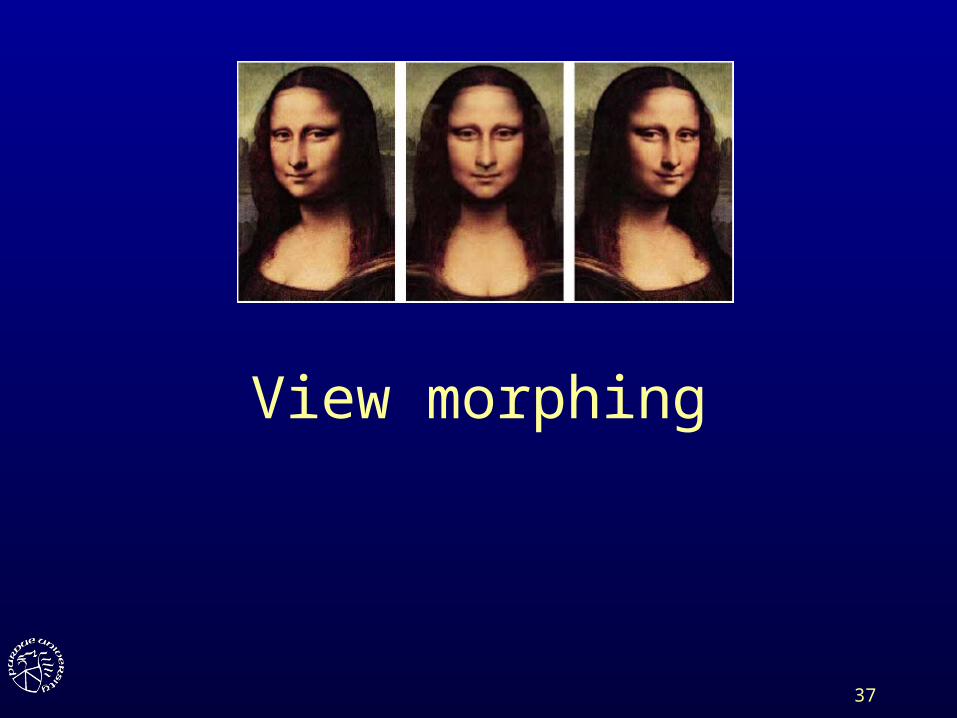
Image Based Rendering
an overview
2
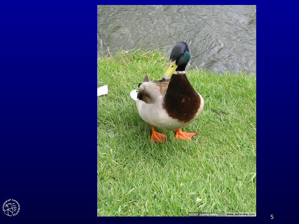
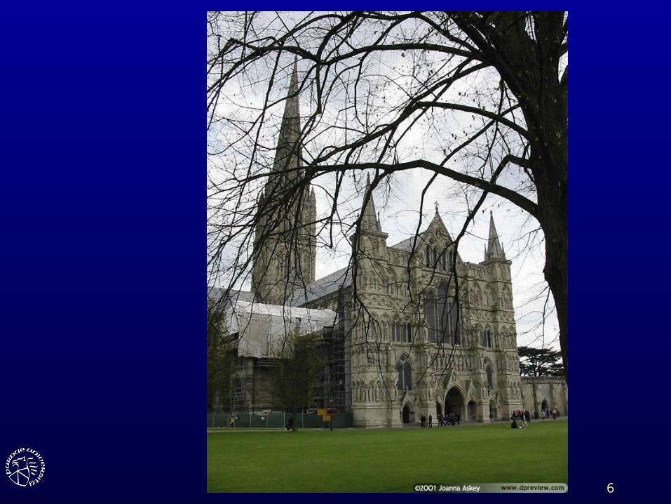
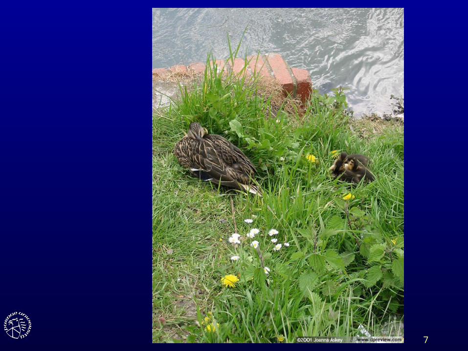
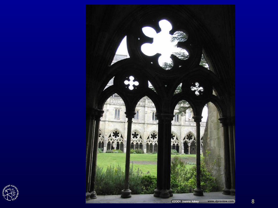
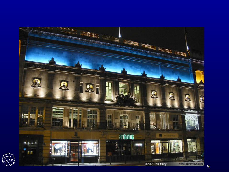
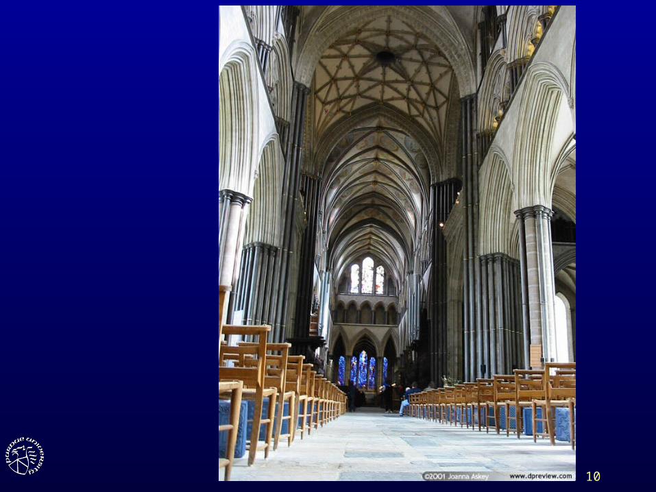
Photographs
• We have tools that acquire and tools that display photographs at a convincing quality level

3

4
5
6
7
8
9
10
11
Photographs
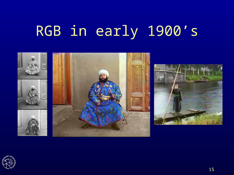
• We have tools that acquire and tools that display photographs at a convincing quality level, for almost 100 years now
12
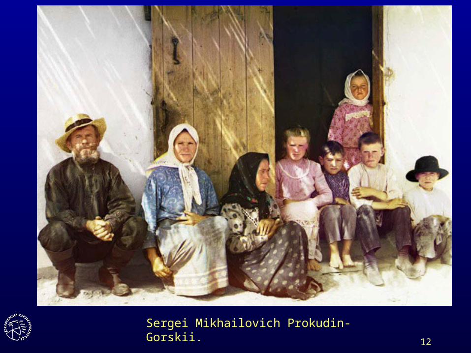
Sergei Mikhailovich Prokudin-Gorskii.
A Settler's Family, ca. 1907-1915.
13
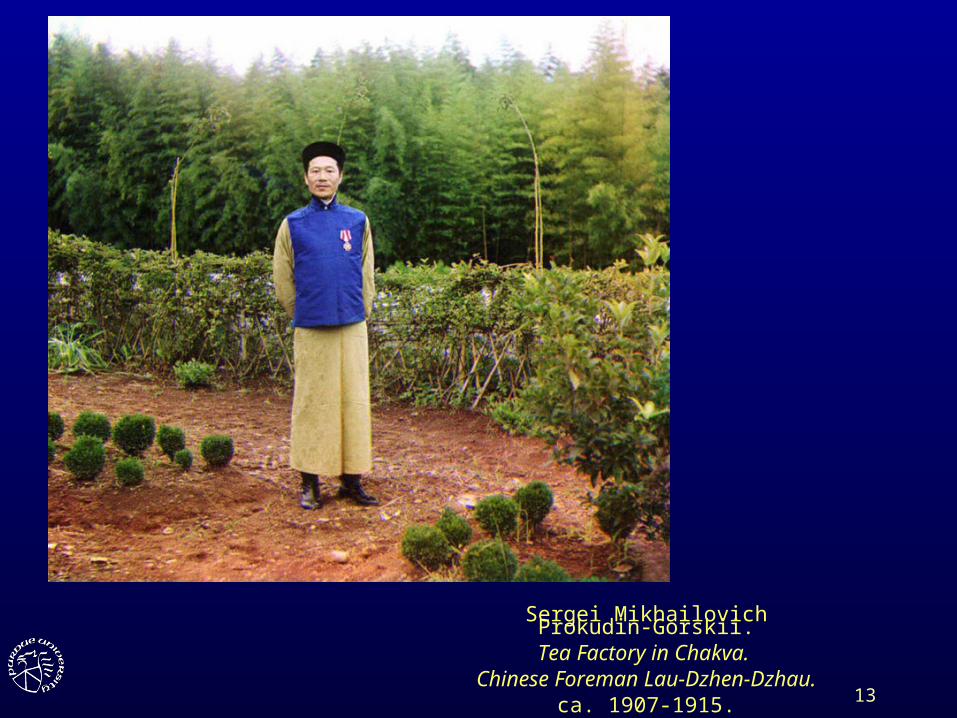
Sergei Mikhailovich Prokudin-Gorskii.Tea Factory in Chakva.
Chinese Foreman Lau-Dzhen-Dzhau.ca. 1907-1915.
14
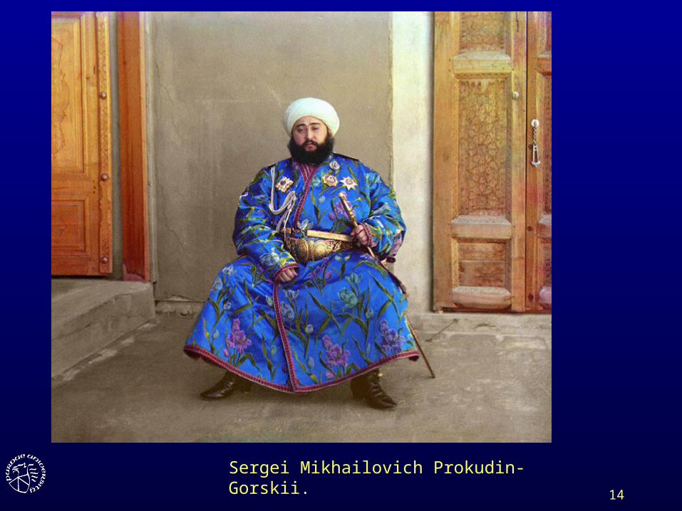
Sergei Mikhailovich Prokudin-Gorskii.
The Emir of Bukhara, 1911.
15
RGB in early 1900’s
16
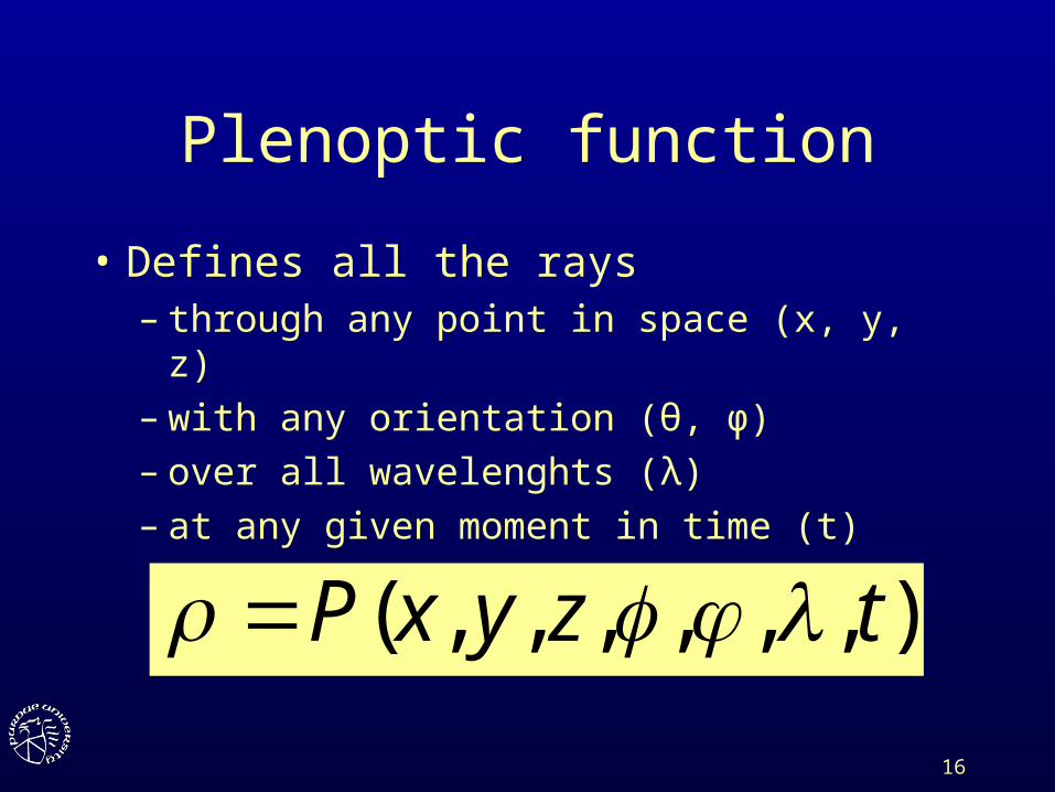
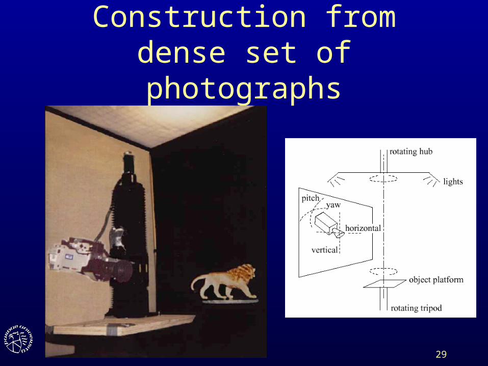
Plenoptic function
• Defines all the rays– through any point in space (x, y, z)– with any orientation (θ, φ)– over all wavelenghts (λ)– at any given moment in time (t)
),,,,,,( tzyxP
17
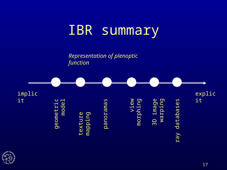
IBR summary
explicitimplicit
geom
etri
c m
odel
text
ure
map
ping
pano
ram
as
view
mor
phin
g
3D im
age
war
ping
ray
data
base
s
Representation of plenoptic function
18
Lightfield – Lumigraph approach[Levoy96, Gortler96]
• Take all photographs you will ever need to display
• Model becomes database of rays
• Rendering becomes database querying
19
Overview
• Introduction
• Lightfield – Lumigraph– definition– construction– compression
20
Overview
• Introduction
• Lightfield – Lumigraph– definition– construction– compression
21
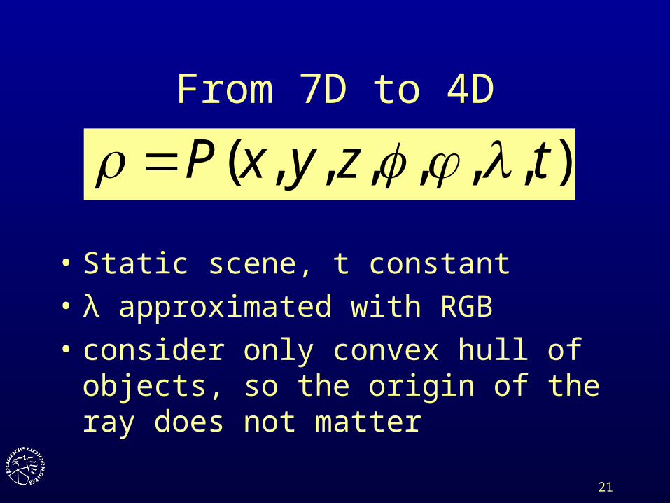
From 7D to 4D
• Static scene, t constant
• λ approximated with RGB
• consider only convex hull of objects, so the origin of the ray does not matter
),,,,,,( tzyxP
22
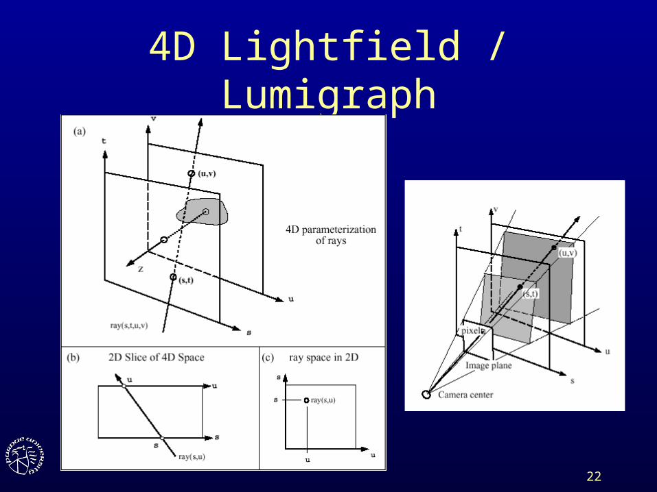
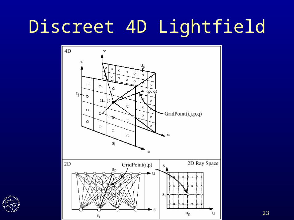
4D Lightfield / Lumigraph
23
Discreet 4D Lightfield
24
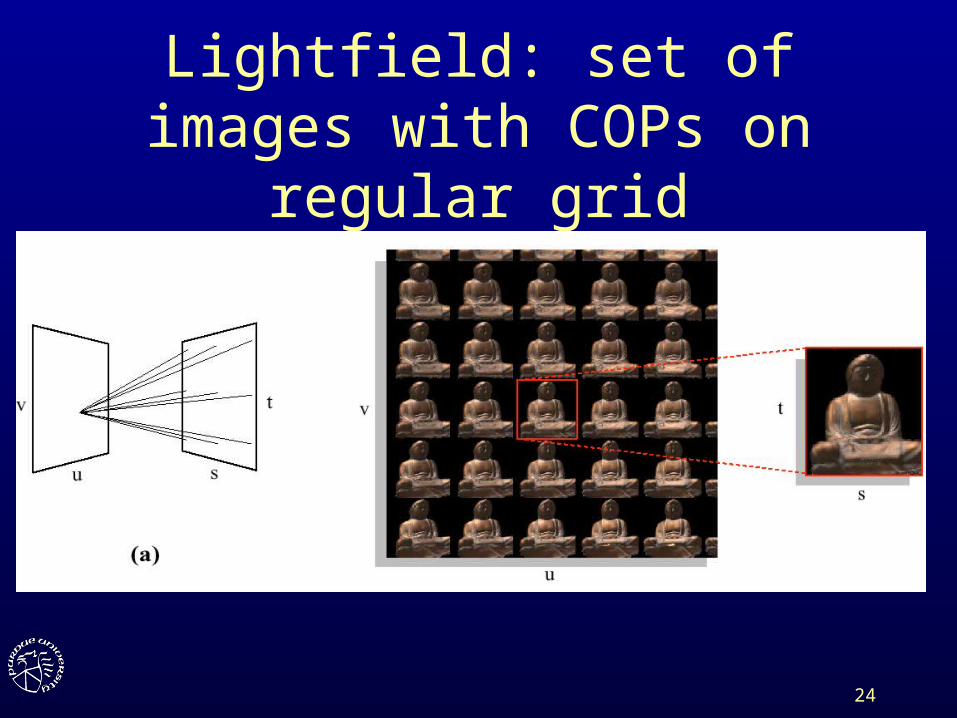
Lightfield: set of images with COPs on regular grid
25
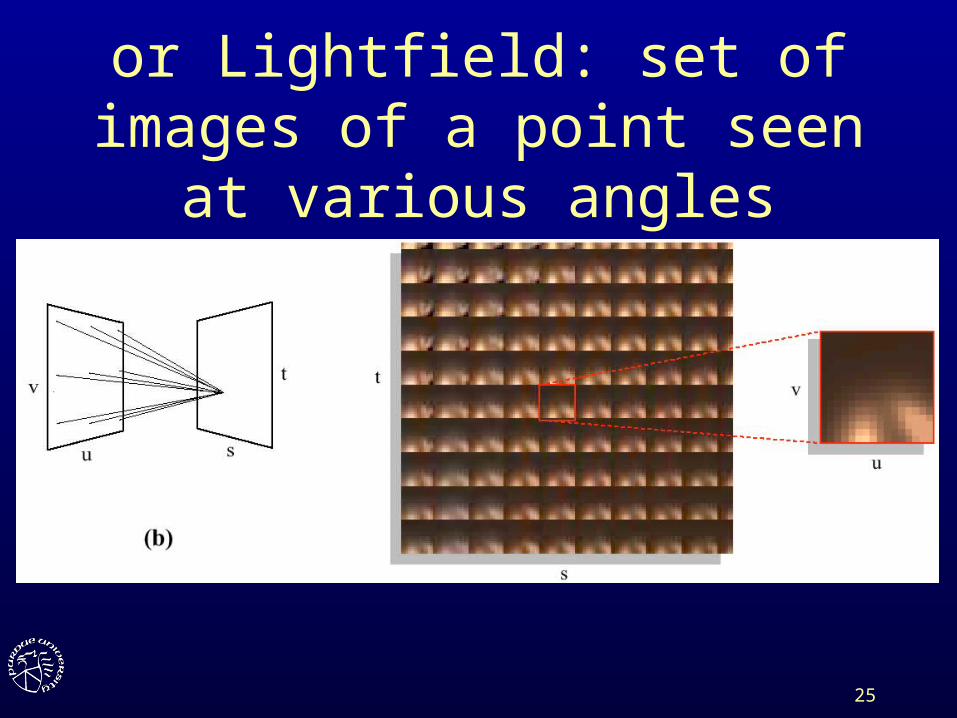
or Lightfield: set of images of a point seen at various angles
26
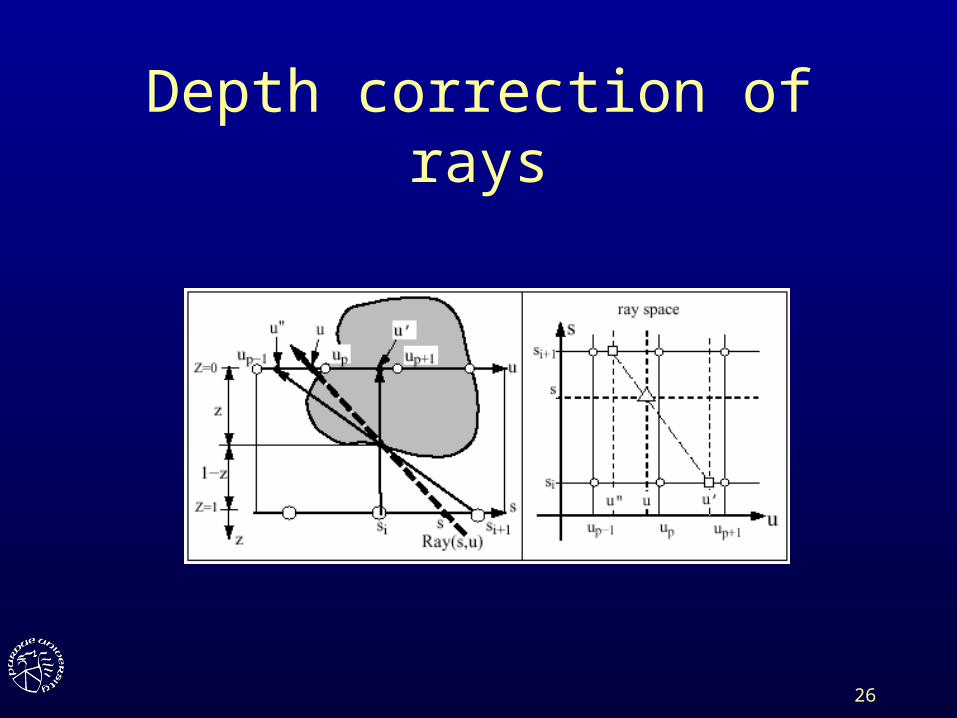
Depth correction of rays

27
Overview
• Introduction
• Lightfield – Lumigraph– definition– construction– compression

28
Overview
• Introduction
• Lightfield – Lumigraph– definition– construction– compression
29
Construction from dense set of photographs
30
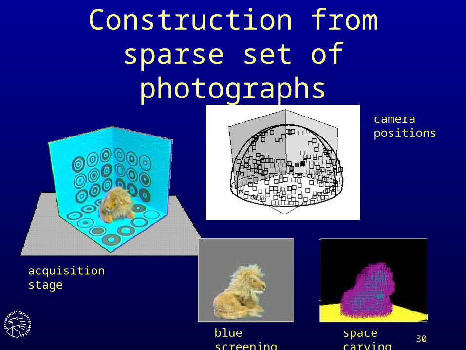
Construction from sparse set of photographs
acquisition stage
camera positions
blue screening space carving
31
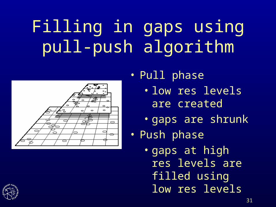
Filling in gaps using pull-push algorithm
• Pull phase • low res levels are
created• gaps are shrunk
• Push phase• gaps at high res levels
are filled using low res levels
32
Overview
• Introduction
• Lightfield – Lumigraph– definition– construction– compression
33
Overview
• Introduction
• Lightfield – Lumigraph– definition– construction– compression
34
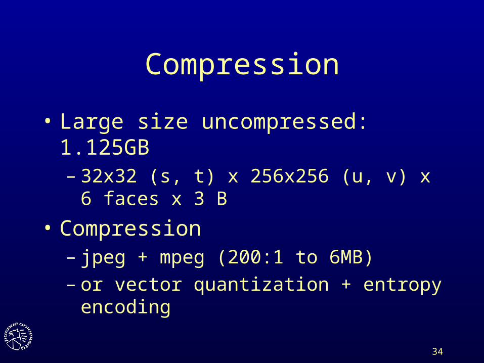
Compression
• Large size uncompressed: 1.125GB– 32x32 (s, t) x 256x256 (u, v) x 6 faces x 3 B
• Compression– jpeg + mpeg (200:1 to 6MB)– or vector quantization + entropy encoding
35
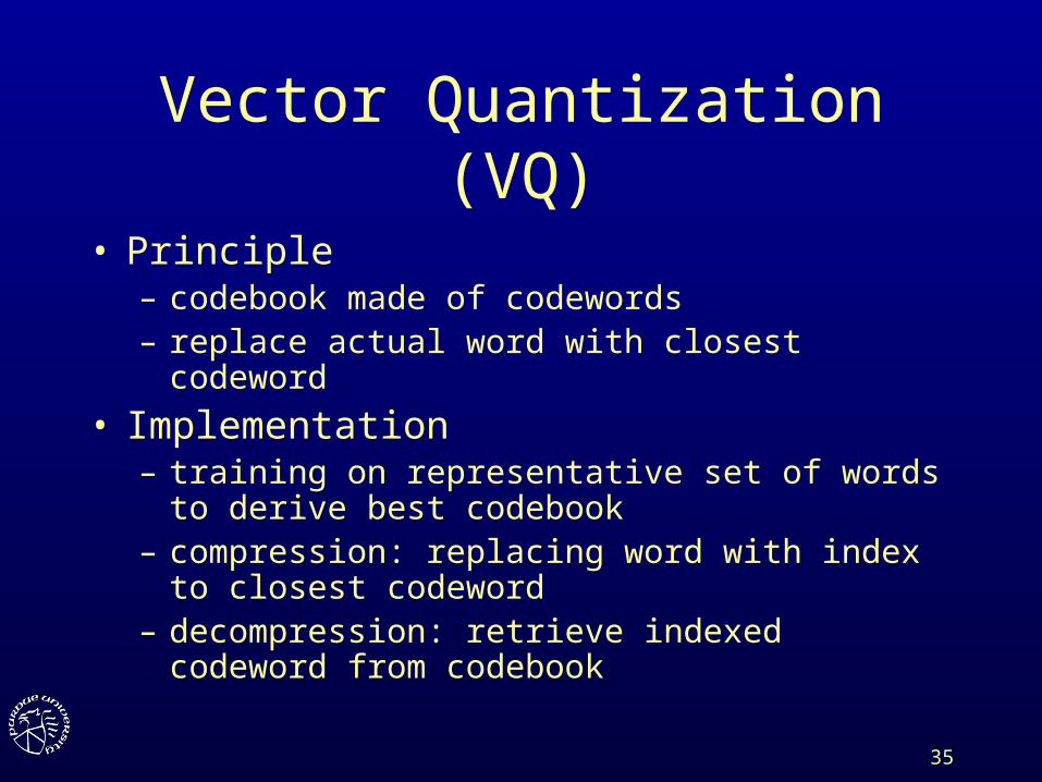
Vector Quantization (VQ)
• Principle– codebook made of codewords– replace actual word with closest codeword
• Implementation– training on representative set of words to derive best
codebook– compression: replacing word with index to closest
codeword– decompression: retrieve indexed codeword from
codebook
36
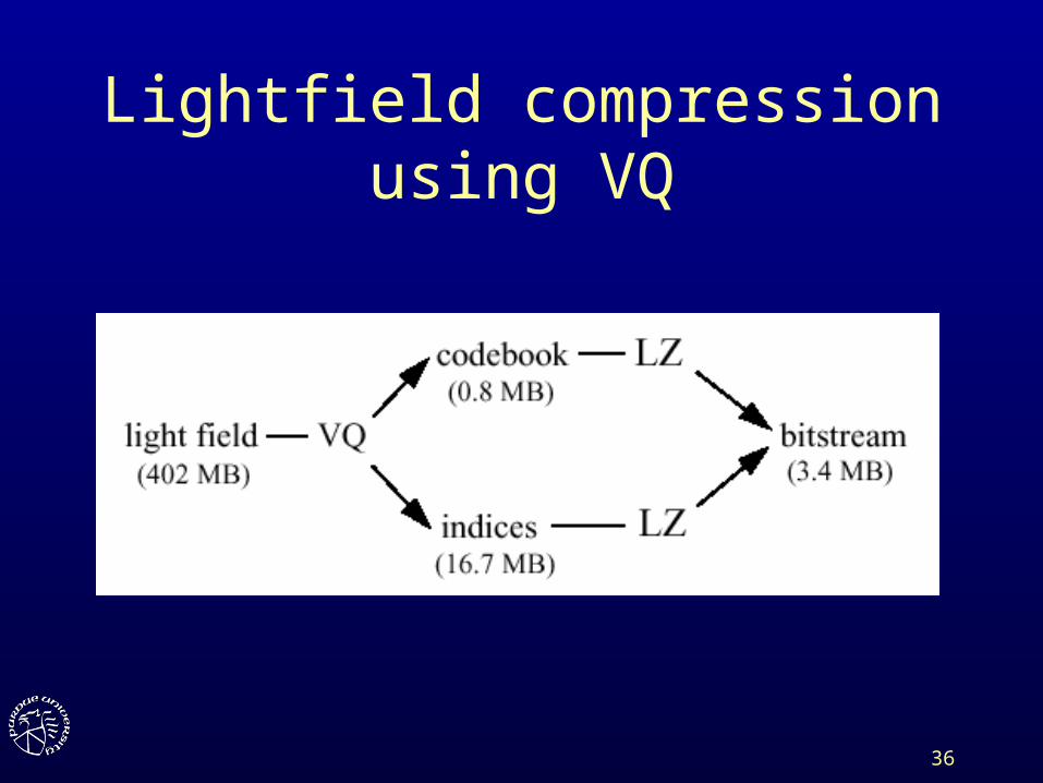
Lightfield compression using VQ
38
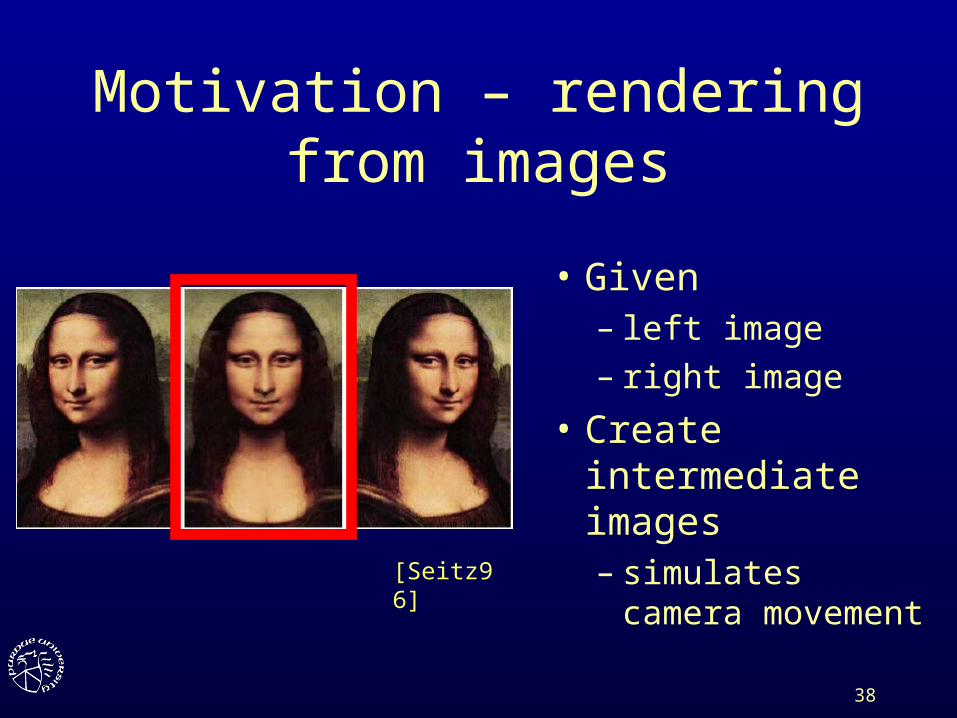
Motivation – rendering from images
• Given– left image– right image
• Create intermediate images– simulates camera
movement[Seitz96]
39
Previous work
• Panoramas ([Chen95], etc)– user can look in any direction at few given locations
• Image-morphing ([Wolberg90], [Beier92], etc)– linearly interpolated intermediate positions of features
– input: two images and correspondences
– output: metamorphosis of one image into other as sequence of intermediate images
40
Previous work limitations
• Panoramas ([Chen95], etc.)– no camera translations allowed
• Image morphing ([Wolberg90], [Beier92], etc.)– not shape-preserving– image morphing is also a morph of the object– to simulate rendering with morphing, the object
should be rigid when camera moves
41
Overview
• Introduction
• Image morphing
• View morphing– image pre-warping– image morphing– image post-warping
42
Overview
• Introduction
• Image morphing
• View morphing– image pre-warping– image morphing– image post-warping

43
Image morphing
1. Correspondences

44
Image morphing
1. Correspondences
45
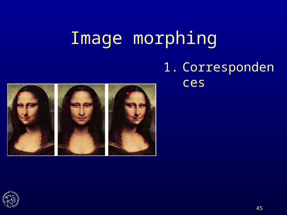
Image morphing
1. Correspondences

46
Image morphing
1. Correspondences
47
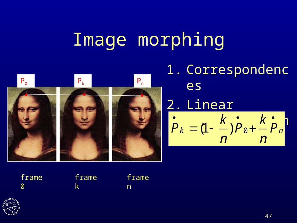
Image morphing
1. Correspondences
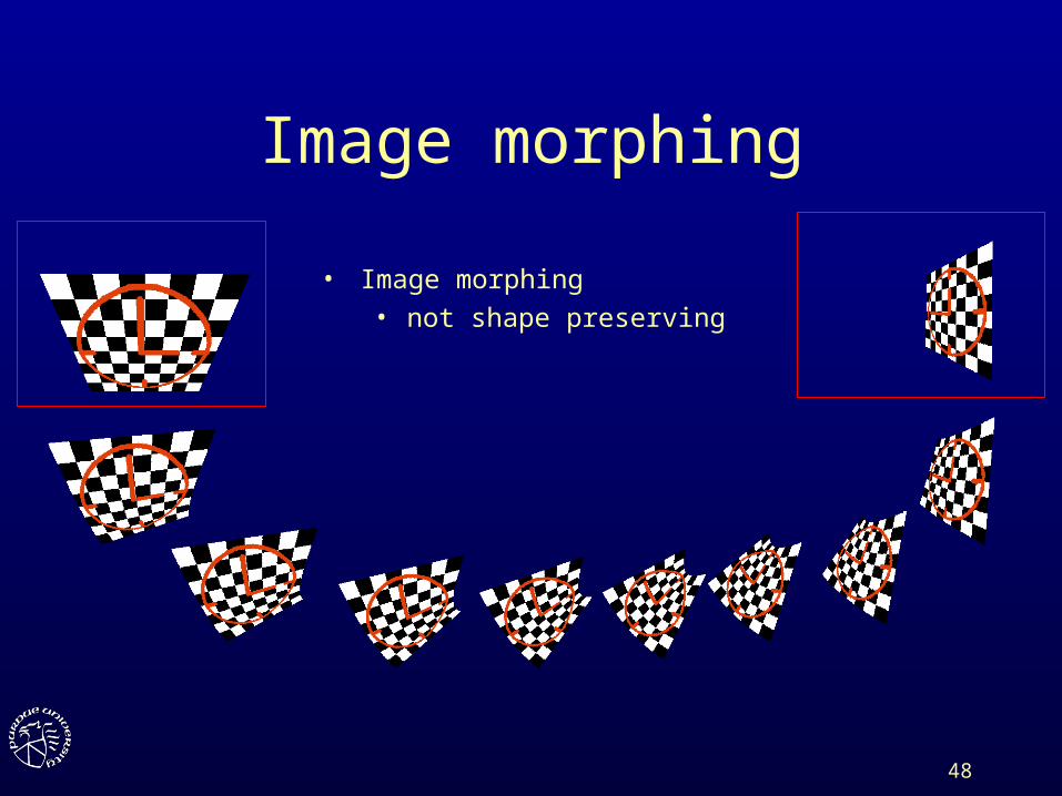
2. Linear interpolation
nk Pn
kP
n
kP
0)1(
P0 Pk Pn
frame 0 frame k frame n
48
Image morphing
• Image morphing
• not shape preserving
49
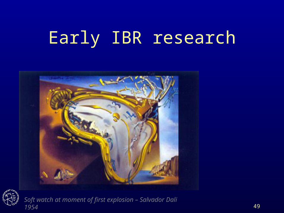
Early IBR research
Soft watch at moment of first explosion – Salvador Dali 1954
50
Overview
• Introduction
• Image morphing
• View morphing– image pre-warping– image morphing– image post-warping
51
Overview
• Introduction
• Image morphing
• View morphing– image pre-warping– image morphing– image post-warping
52
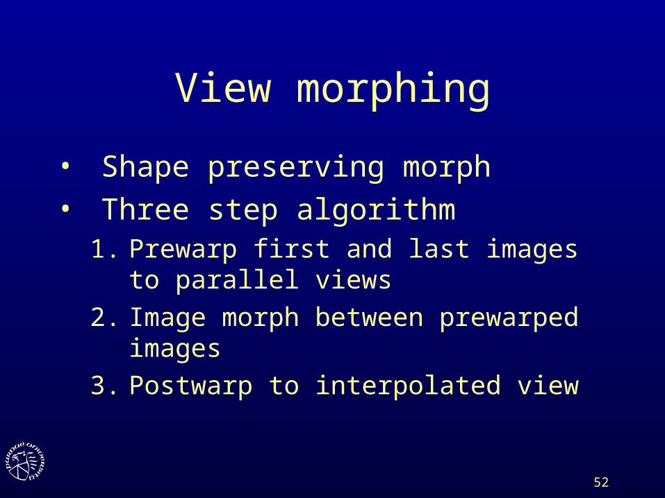
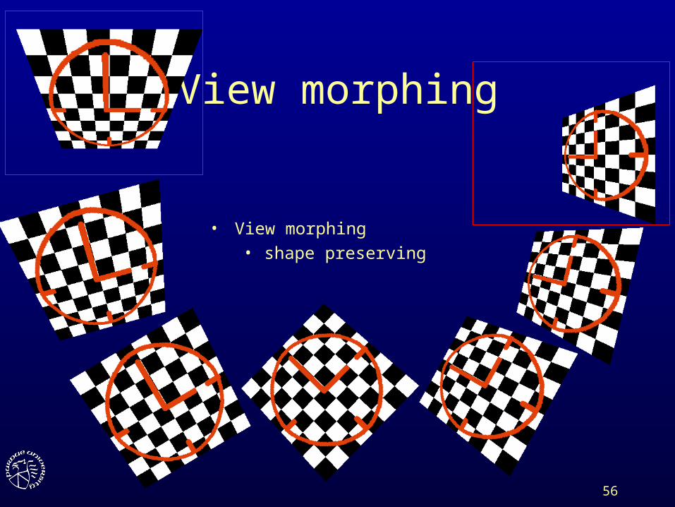
View morphing
• Shape preserving morph
• Three step algorithm1. Prewarp first and last images to parallel views
2. Image morph between prewarped images
3. Postwarp to interpolated view
53
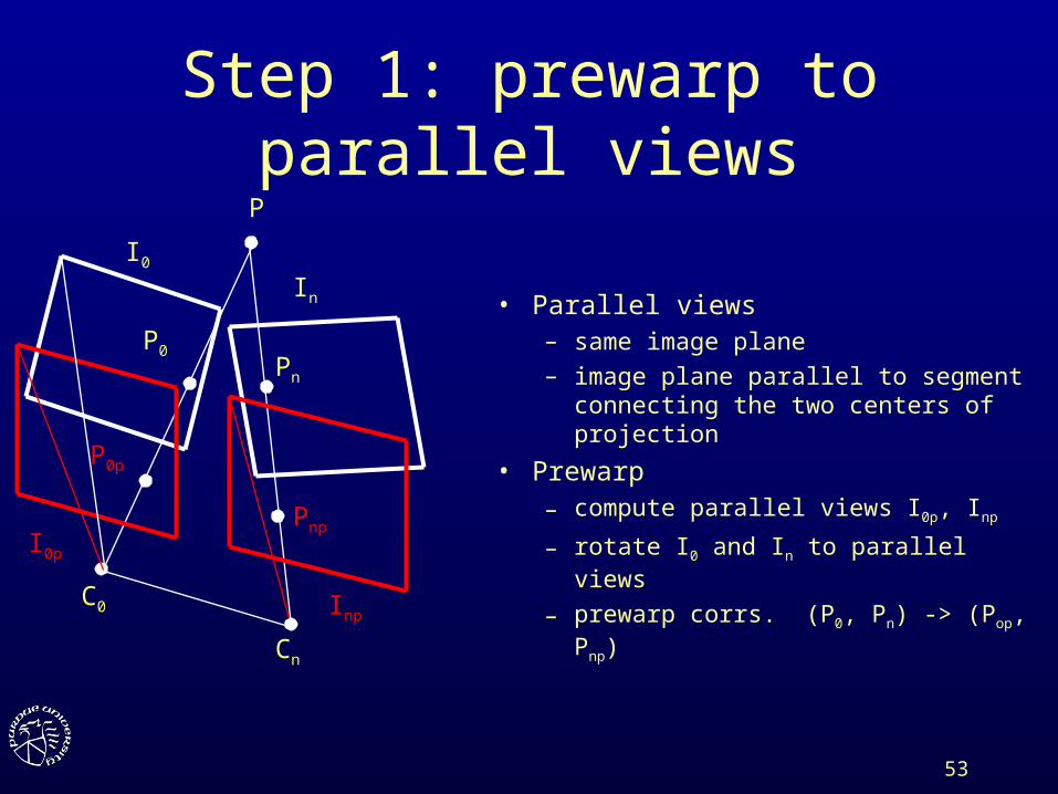
Step 1: prewarp to parallel views
• Parallel views– same image plane
– image plane parallel to segment connecting the two centers of projection
• Prewarp– compute parallel views I0p, Inp
– rotate I0 and In to parallel views
– prewarp corrs. (P0, Pn) -> (Pop, Pnp)
Cn
C0
I0
In
Inp
I0p
P
P0 Pn
P0p
Pnp
54
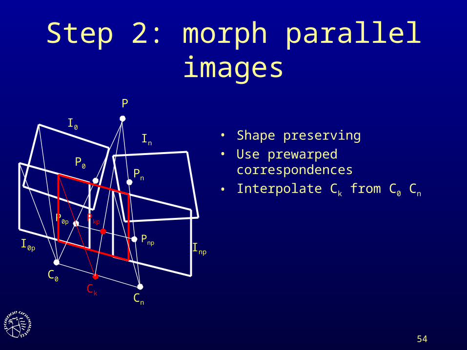
Step 2: morph parallel images
• Shape preserving
• Use prewarped correspondences
• Interpolate Ck from C0 Cn
Cn
C0
I0
In
InpI0p
P
P0 Pn
P0p
Pnp
Ck
Pkp
55
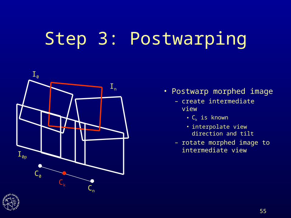
Step 3: Postwarping
• Postwarp morphed image– create intermediate view
• Ck is known
• interpolate view direction and tilt
– rotate morphed image to intermediate view
Cn
C0
I0
In
I0p
Ck
56
View morphing
• View morphing
• shape preserving

57
Overview
• Introduction
• Image morphing
• View morphing, more details– image pre-warping– image morphing– image post-warping
58
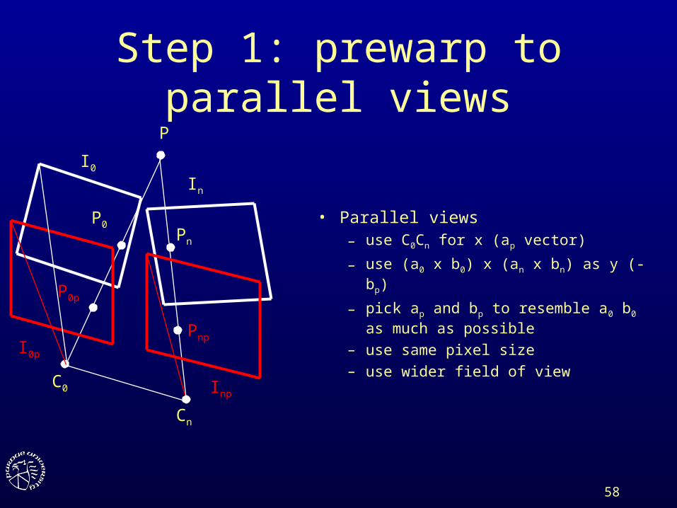
Step 1: prewarp to parallel views
• Parallel views– use C0Cn for x (ap vector)
– use (a0 x b0) x (an x bn) as y (-bp)
– pick ap and bp to resemble a0 b0 as much as possible
– use same pixel size
– use wider field of view
Cn
C0
I0
In
Inp
I0p
P
P0 Pn
P0p
Pnp
59
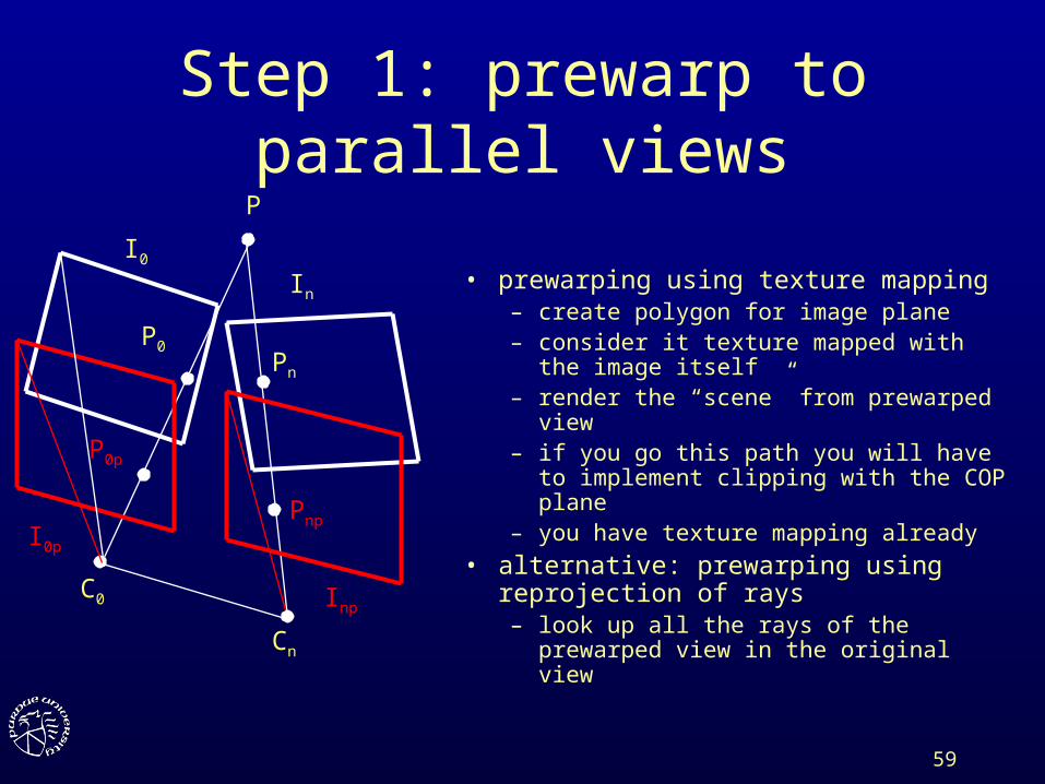
Step 1: prewarp to parallel views
• prewarping using texture mapping– create polygon for image plane– consider it texture mapped with the image
itself– render the “scene” from prewarped view– if you go this path you will have to
implement clipping with the COP plane– you have texture mapping already
• alternative: prewarping using reprojection of rays– look up all the rays of the prewarped view
in the original viewCn
C0
I0
In
Inp
I0p
P
P0 Pn
P0p
Pnp
60
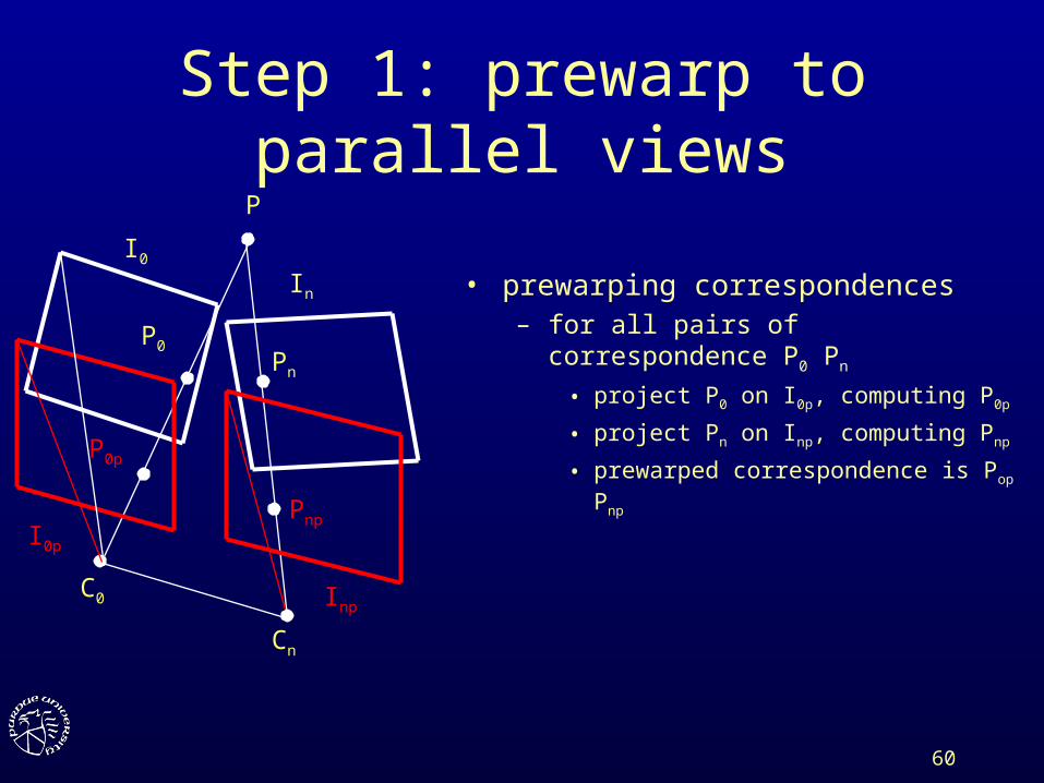
Step 1: prewarp to parallel views
• prewarping correspondences– for all pairs of correspondence P0 Pn
• project P0 on I0p, computing P0p
• project Pn on Inp, computing Pnp
• prewarped correspondence is Pop Pnp
Cn
C0
I0
In
Inp
I0p
P
P0 Pn
P0p
Pnp
61
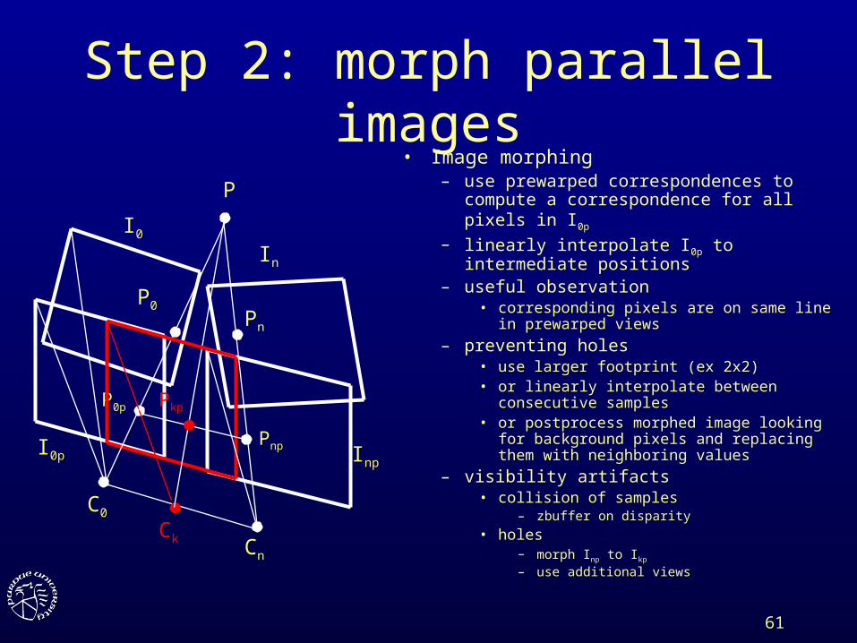
Step 2: morph parallel images• Image morphing
– use prewarped correspondences to compute a correspondence for all pixels in I0p
– linearly interpolate I0p to intermediate positions– useful observation
• corresponding pixels are on same line in prewarped views
– preventing holes• use larger footprint (ex 2x2)• or linearly interpolate between consecutive
samples• or postprocess morphed image looking for
background pixels and replacing them with neighboring values
– visibility artifacts• collision of samples
– zbuffer on disparity
• holes– morph Inp to Ikp
– use additional views
Cn
C0
I0
In
InpI0p
P
P0 Pn
P0p
Pnp
Ck
Pkp
62
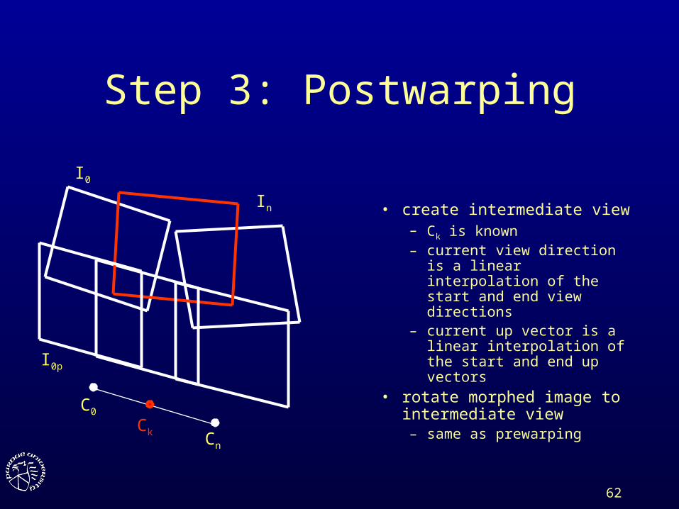
Step 3: Postwarping
• create intermediate view– Ck is known– current view direction is a
linear interpolation of the start and end view directions
– current up vector is a linear interpolation of the start and end up vectors
• rotate morphed image to intermediate view– same as prewarping
Cn
C0
I0
In
I0p
Ck
63
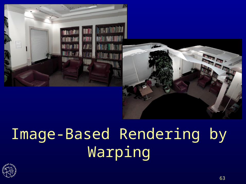
Image-Based Rendering by Warping
64
Overview
• Introduction
• Depth extraction methods
• Reconstruction for IBRW
• Visibility without depth
• Sample selection
65
Overview
• Introduction– comparison to other IBR methods– 3D warping equation– reconstruction
66
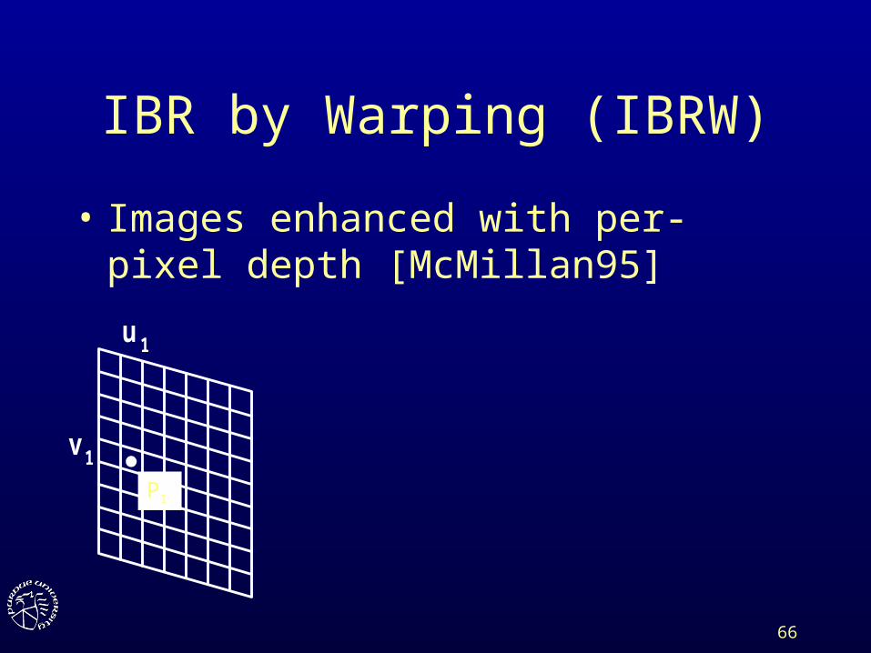
IBR by Warping (IBRW)
• Images enhanced with per-pixel depth [McMillan95]
u1
v1P1
67
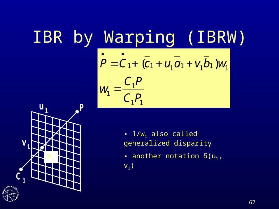
IBR by Warping (IBRW)
C1
Pu1
v1
11
11
1111111 )(
PC
PCw
wbvaucCP
P1
• 1/w1 also called generalized disparity
• another notation δ(u1, v1)
68
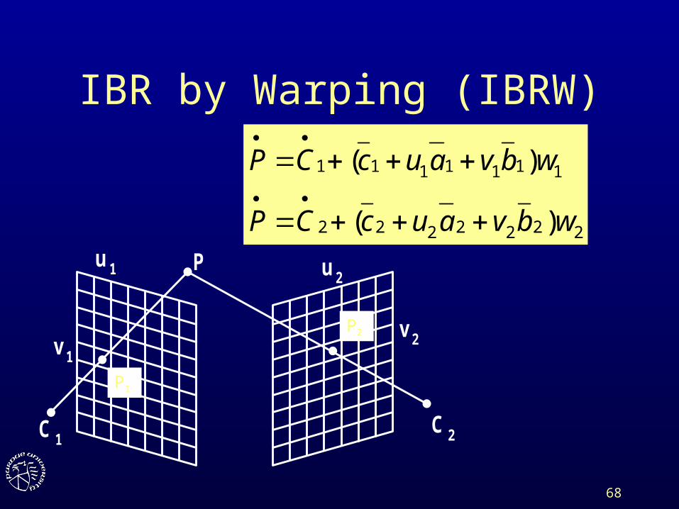
IBR by Warping (IBRW)
C1
P
C2
u2
v2
u1
v1
2222222
1111111
)(
)(
wbvaucCP
wbvaucCP
P1
P2
69
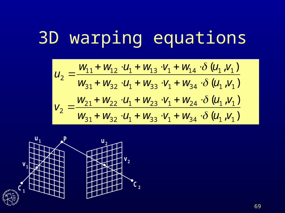
3D warping equations
C1
P
C2
u2
v2
u1
v1
),(
),(
),(
),(
113413313231
1124123122212
113413313231
1114113112112
vuwvwuww
vuwvwuwwv
vuwvwuww
vuwvwuwwu
70
A complete IBR method
• Façade system– (coarse) geometric model needed
• Panoramas– viewer confined to center of panorama
• View morphing– correspondences needed
• IBRW– rendering to arbitrary new views
71
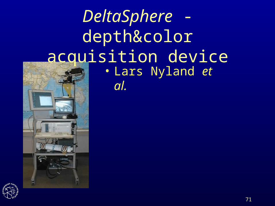
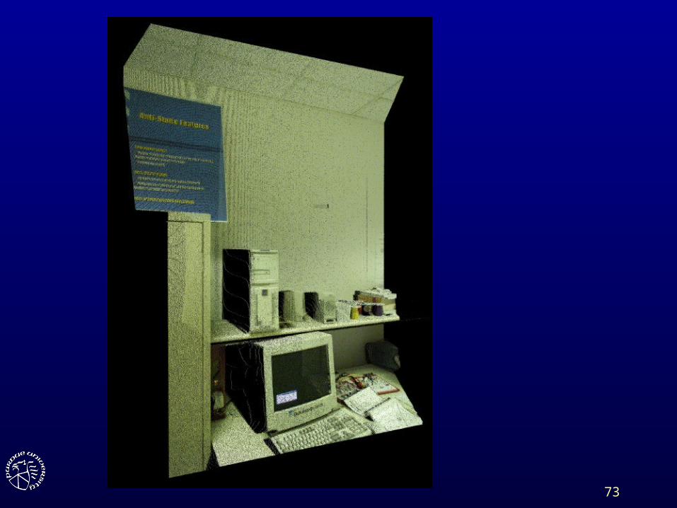
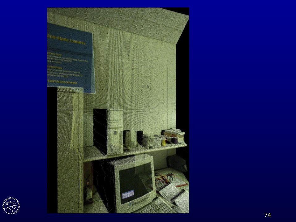
DeltaSphere - depth&color acquisition device
• Lars Nyland et al.
72
73
74
75
76
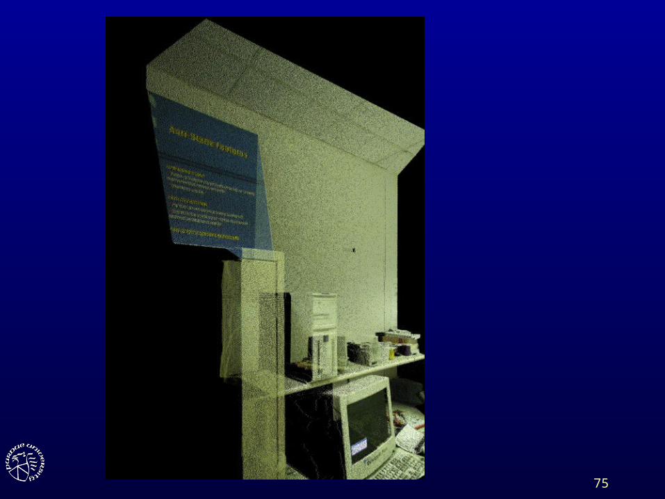
Reconstructing by splatting
• Estimate shape and size of footprint of warped samples– expensive to do accurately– lower image quality if crudely approximated
• Samples are z-buffered
77
Overview
• Introduction
• Depth extraction methods
• Reconstruction for IBRW
• Visibility without depth
• Sample selection
78
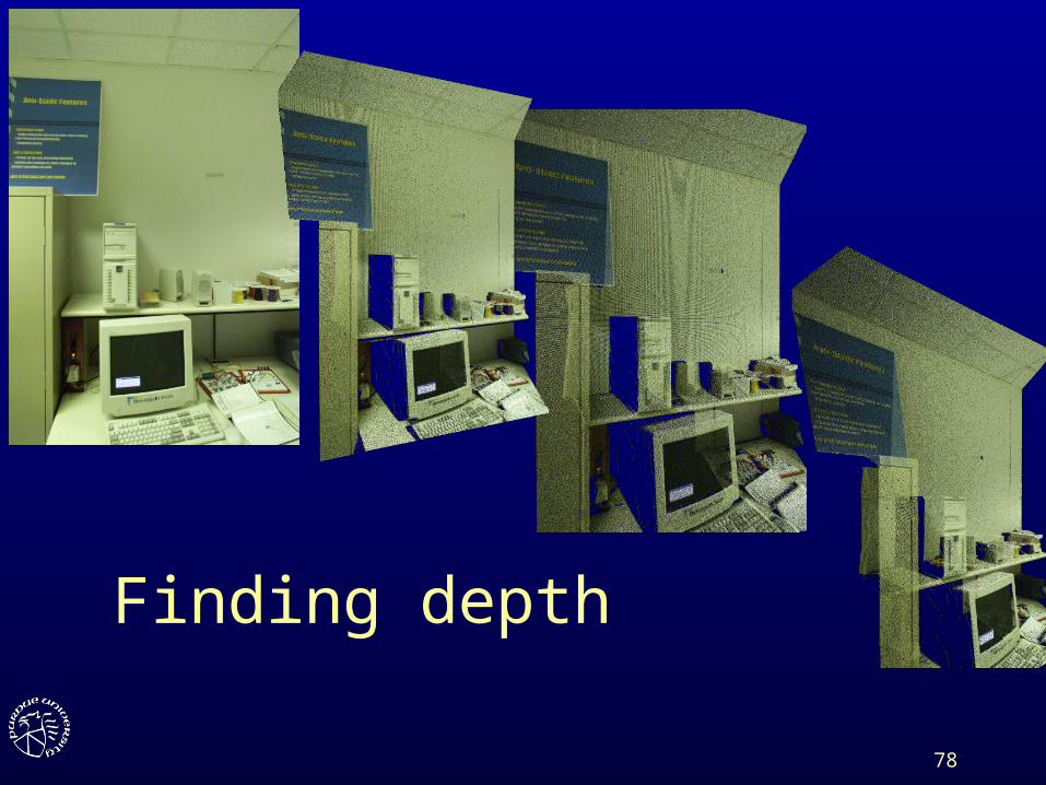
Finding depth
79
Overview
• Depth from stereo
• Depth from structured light
• Depth from focus / defocus
• Laser rangefinders

80
Overview
• Depth from stereo
• Depth from structured light
• Depth from focus / defocus
• Laser rangefinders
81
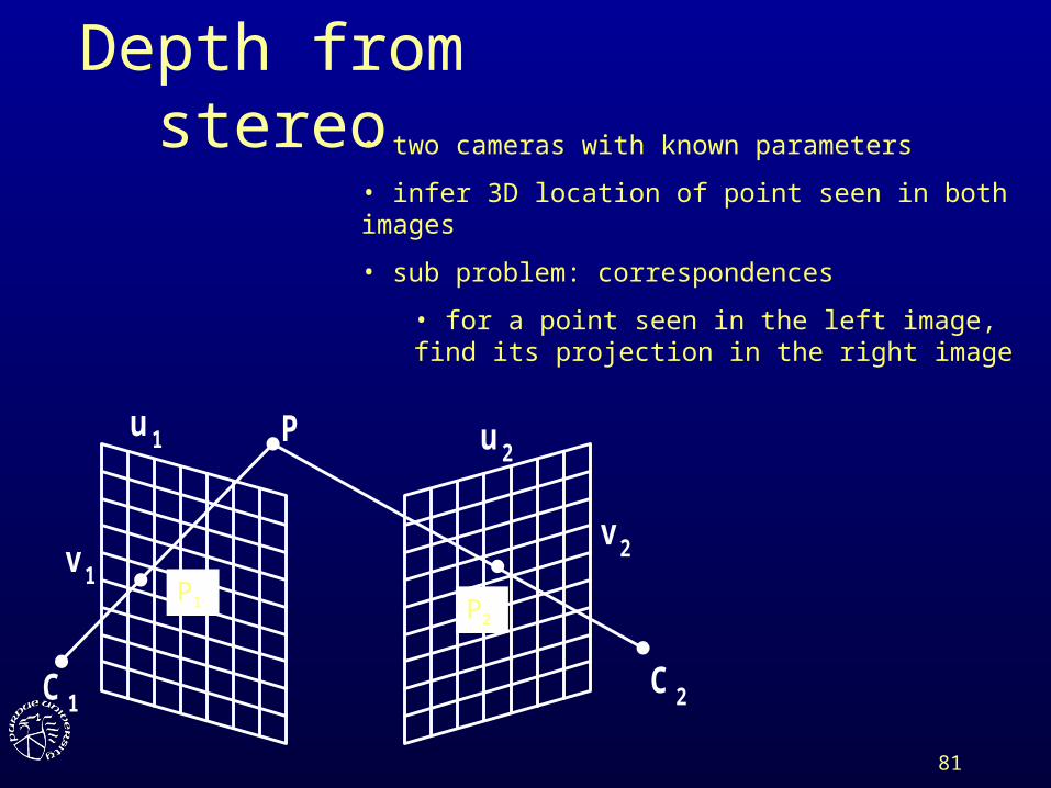
Depth from stereo
C1
P
C2
u2
v2
u1
v1P1 P2
• two cameras with known parameters
• infer 3D location of point seen in both images
• sub problem: correspondences
• for a point seen in the left image, find its projection in the right image
82
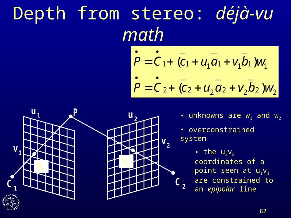
Depth from stereo: déjà-vu math
C1
P
C2
u2
v2
u1
v1
2222222
1111111
)(
)(
wbvaucCP
wbvaucCP
P1
P2
• unknowns are w1 and w2
• overconstrained system
• the u2v2 coordinates of a point seen at u1v1 are constrained to an epipolar line
83
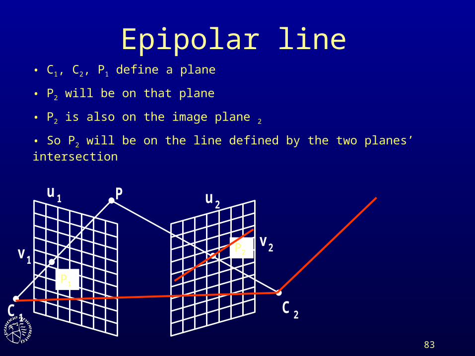
Epipolar line
C1
P
C2
u2
v2
u1
v1P1
P2
• C1, C2, P1 define a plane
• P2 will be on that plane
• P2 is also on the image plane 2
• So P2 will be on the line defined by the two planes’ intersection
84
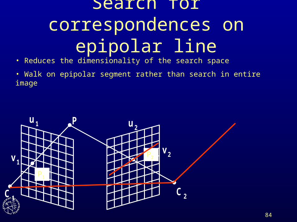
Search for correspondences on epipolar line
C1
P
C2
u2
v2
u1
v1P1
P2
• Reduces the dimensionality of the search space
• Walk on epipolar segment rather than search in entire image
85
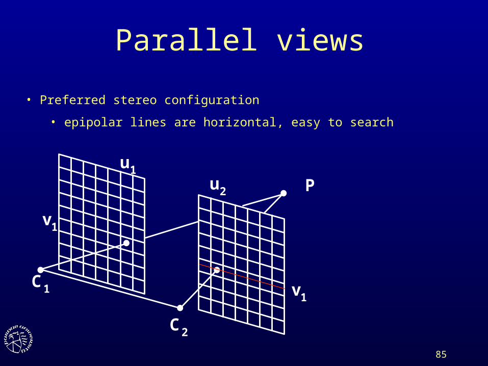
Parallel views
C1
P
C2
u2
v1
u1
v1
• Preferred stereo configuration
• epipolar lines are horizontal, easy to search
86
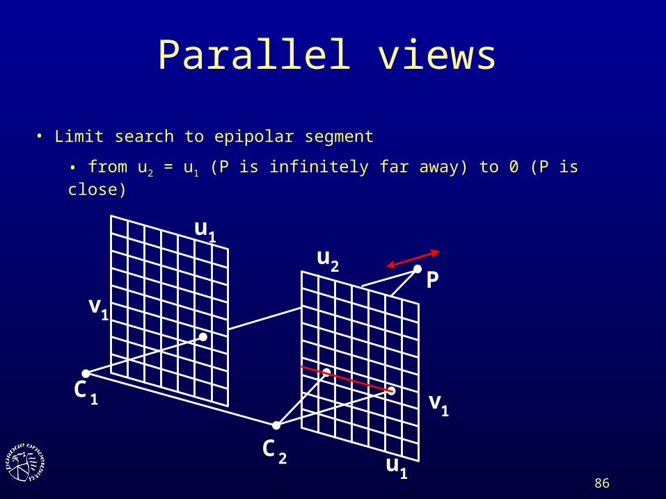
Parallel views
C1
P
C2
u2
v1
u1
v1
u1
• Limit search to epipolar segment
• from u2 = u1 (P is infinitely far away) to 0 (P is close)
87
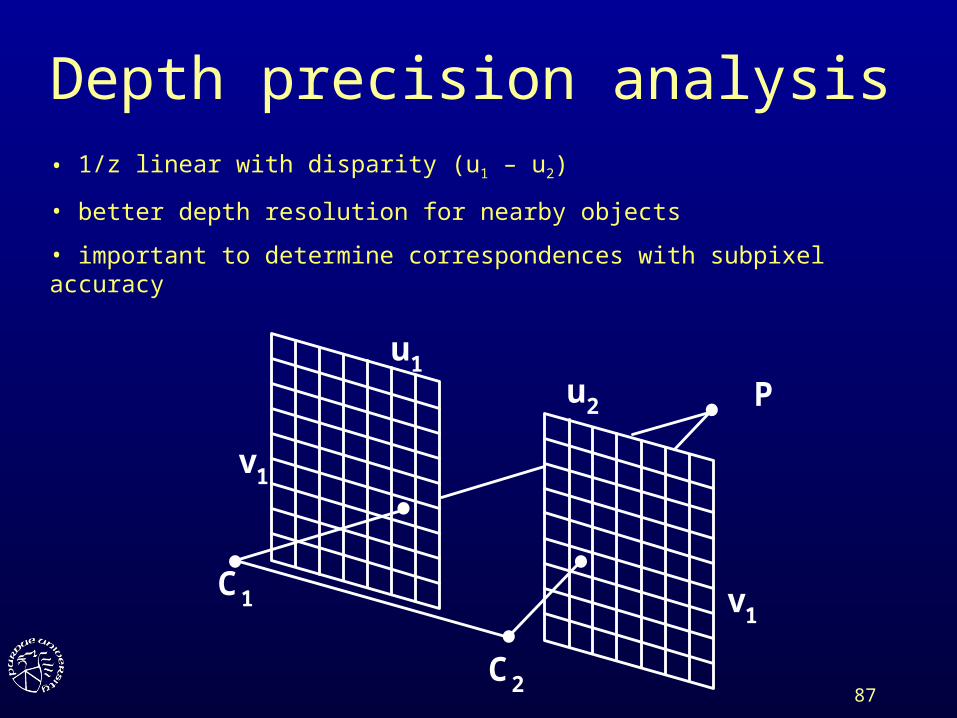
Depth precision analysis
C1
P
C2
u2
v1
u1
v1
• 1/z linear with disparity (u1 – u2)
• better depth resolution for nearby objects
• important to determine correspondences with subpixel accuracy
88
Overview
• Depth from stereo
• Depth from structured light
• Depth from focus / defocus
• Laser rangefinders
89
Overview
• Depth from stereo
• Depth from structured light
• Depth from focus / defocus
• Laser rangefinders
90
Depth from stereo problem
• Correspondences are difficult to find
• Structured light approach– replace one camera with projector– project easily detectable patterns– establishing correspondences becomes a lot
easier
91
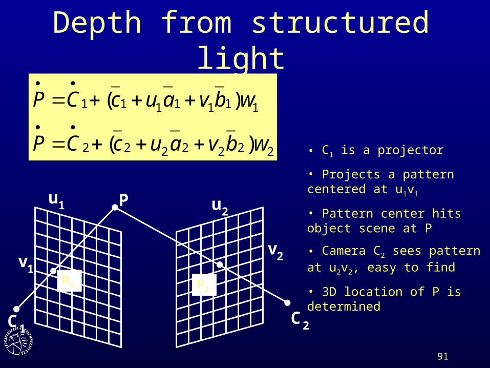
Depth from structured light
C1
P
C2
u2
v2
u1
v1
2222222
1111111
)(
)(
wbvaucCP
wbvaucCP
P1 P2
• C1 is a projector
• Projects a pattern centered at u1v1
• Pattern center hits object scene at P
• Camera C2 sees pattern at u2v2, easy to find
• 3D location of P is determined

93
94
Depth from structured light challenges
• Associated with using projectors– expensive, cannot be used outdoors, not
portable
• Difficult to identify pattern– I found a corner, which corner is it?
• Invasive, change the color of the scene– one could use invisible light, IR

95
Overview
• Depth from stereo
• Depth from structured light
• Depth from focus / defocus
• Laser rangefinders

96
Overview
• Depth from stereo
• Depth from structured light
• Depth from focus / defocus
• Laser rangefinders
97
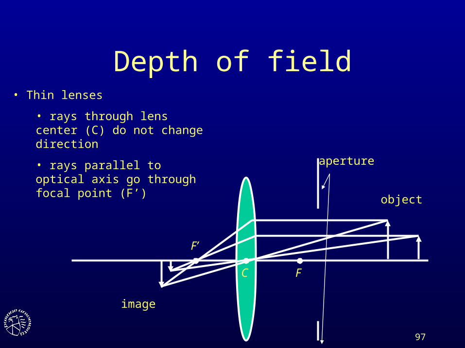
Depth of field
aperture
object
image
C F
F’
• Thin lenses
• rays through lens center (C) do not change direction
• rays parallel to optical axis go through focal point (F’)
98
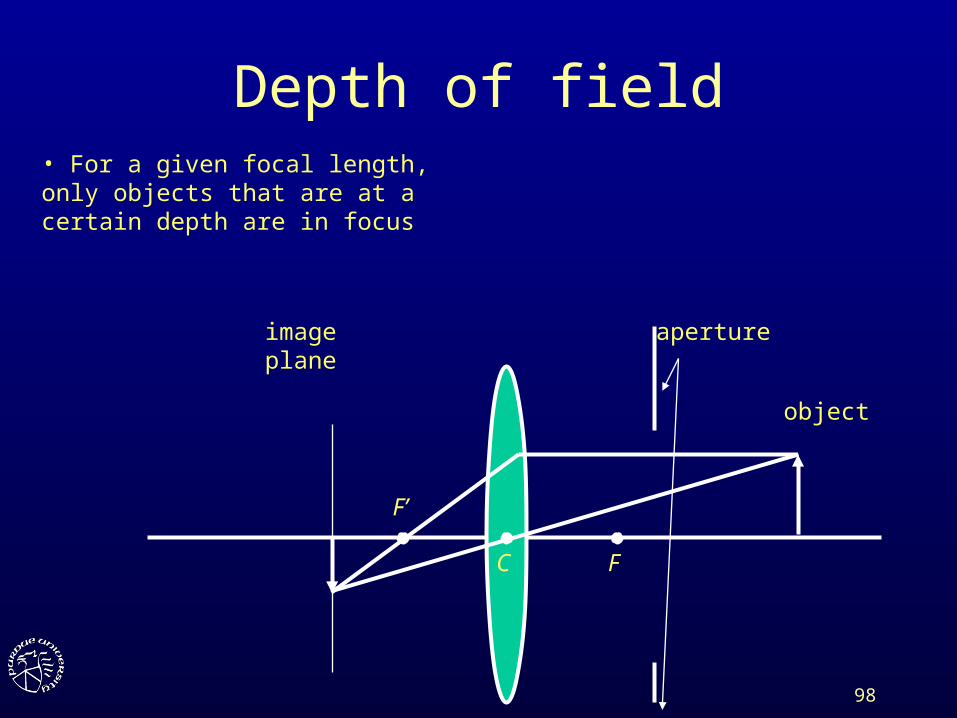
Depth of field
aperture
object
image plane
C F
F’
• For a given focal length, only objects that are at a certain depth are in focus
99
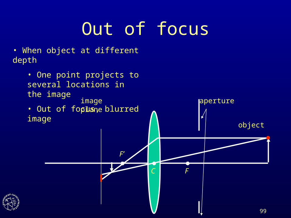
Out of focus
aperture
object
image plane
C F
F’
• When object at different depth
• One point projects to several locations in the image
• Out of focus, blurred image
100
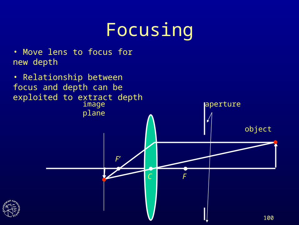
Focusing
aperture
object
image plane
C F
F’
• Move lens to focus for new depth
• Relationship between focus and depth can be exploited to extract depth
101
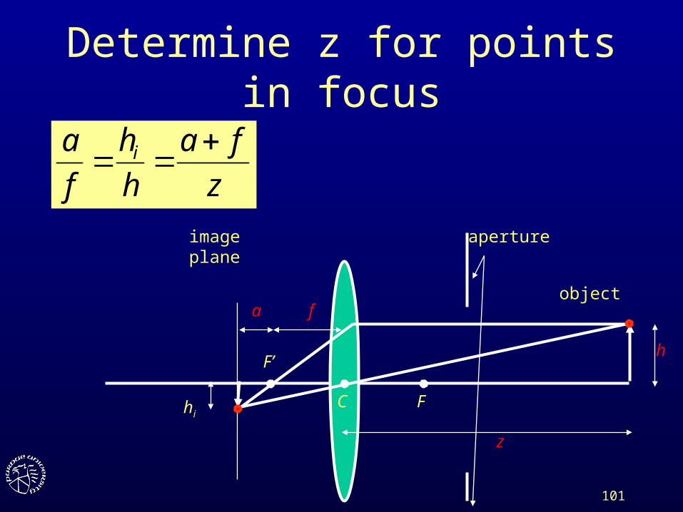
Determine z for points in focus
aperture
object
image plane
C F
F’
z
fa
h
h
f
a i
hi
h
a f
z
102
Depth from defocus
• Take images of a scene with various camera parameters
• Measuring defocus variation, infer range to objects
• Does not need to find the best focusing planes for the various objects
• Examples by Shree Nayar, Columbia U
103
Overview
• Depth from stereo
• Depth from structured light
• Depth from focus / defocus
• Laser rangefinders
104
Overview
• Depth from stereo
• Depth from structured light
• Depth from focus / defocus
• Laser rangefinders
105
Laser range finders
• Send a laser beam to measure the distance– like RADAR, measures time of flight
106
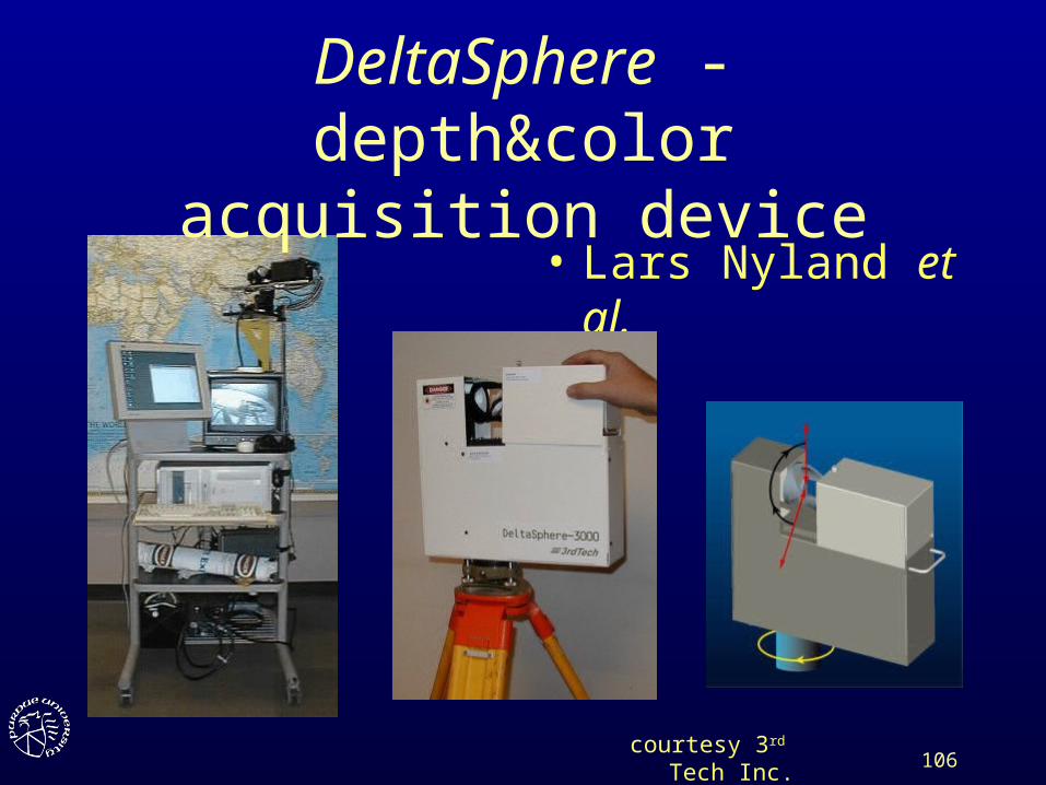
DeltaSphere - depth&color acquisition device
• Lars Nyland et al.
courtesy 3rd Tech Inc.
107
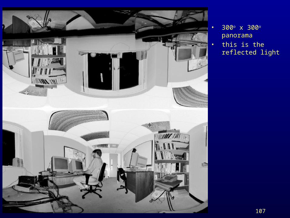
• 300o x 300o panorama
• this is the reflected light
108
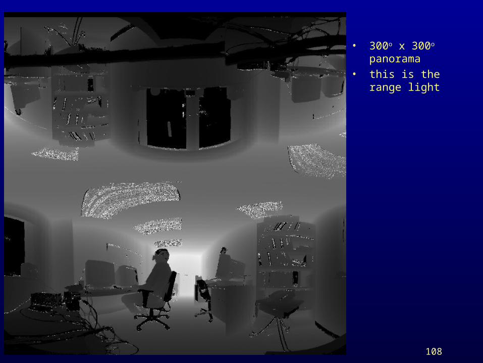
• 300o x 300o panorama
• this is the range light
109
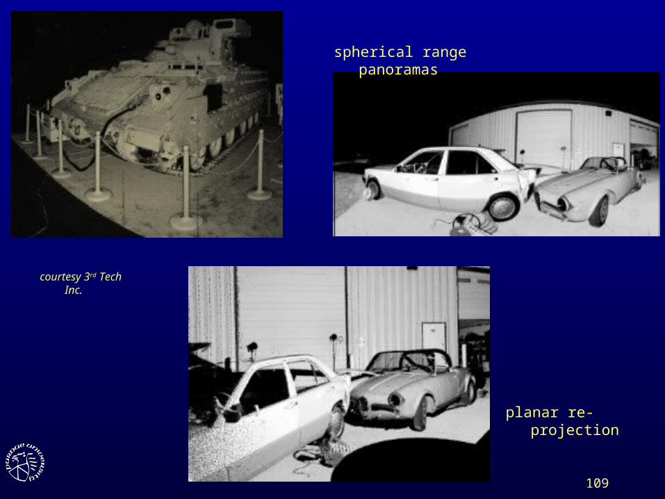
courtesy 3rd Tech Inc.
spherical range panoramas
planar re-projection
110
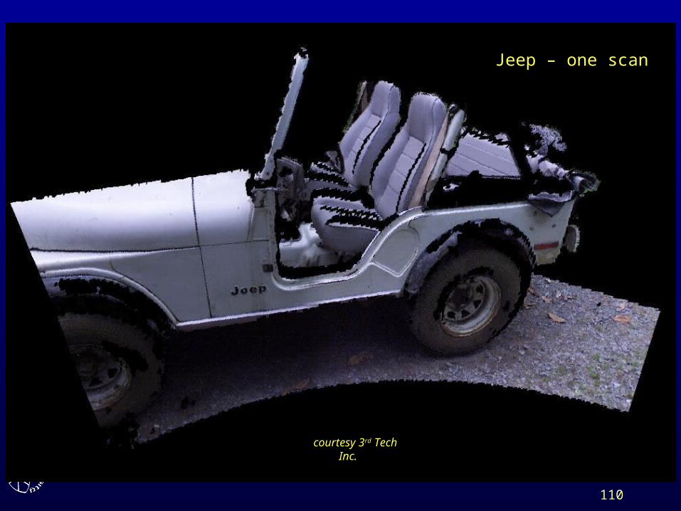
courtesy 3rd Tech Inc.
Jeep – one scan
111
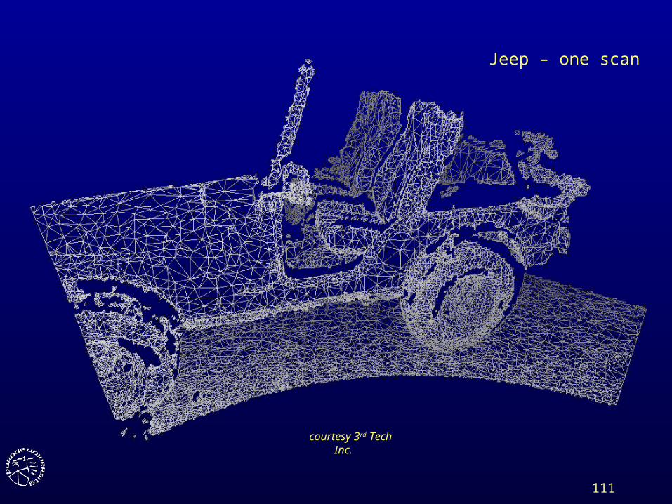
courtesy 3rd Tech Inc.
Jeep – one scan
112
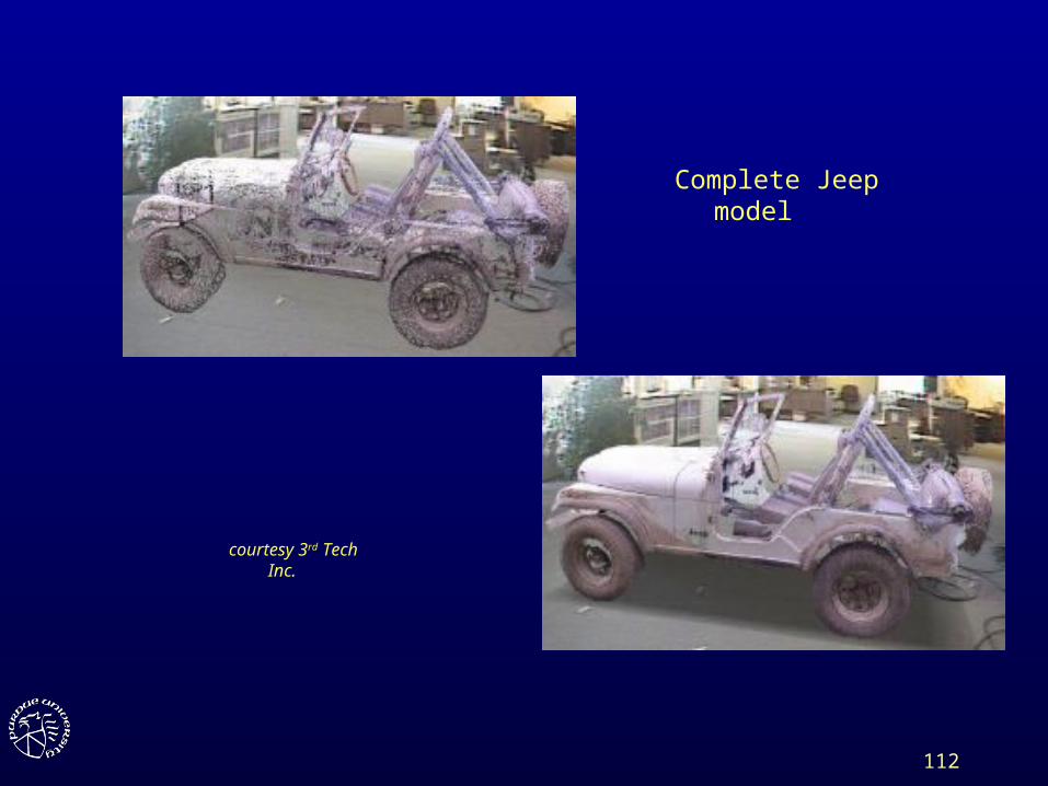
courtesy 3rd Tech Inc.
Complete Jeep model
113