arX

iv:1

711.

0913

9v1

[as

tro-

ph.G

A]

24

Nov

201

7Mon. Not. R. Astron. Soc. 000, 1–14 (2017) Printed 28 November 2017 (MN LATEX style file v2.2)

Galaxy And Mass Assembly (GAMA): the G02 field,

Herschel-ATLAS target selection and Data Release 3

I.K. Baldry,1 J. Liske,2 M.J.I. Brown,3 A.S.G. Robotham,4 S.P. Driver,4,5 L. Dunne,6,7

M. Alpaslan,8,9 S. Brough,10 M.E. Cluver,11 E. Eardley,6 D.J. Farrow,12 C. Heymans,6

H. Hildebrandt,13 A.M. Hopkins,14 L.S. Kelvin,1 J. Loveday,15 A.J. Moffett,16

P. Norberg,17 M.S. Owers,18 E.N. Taylor,19 A.H. Wright,13 S.P. Bamford,20

J. Bland-Hawthorn,21 N. Bourne,6 M.N. Bremer,22 M. Colless,23 C.J. Conselice,20

S.M. Croom,21 L.J.M. Davies,4 C. Foster,14,21 M.W. Grootes,24 B.W. Holwerda,25

D.H. Jones,3 P.R. Kafle,4 K. Kuijken,26 M.A. Lara-Lopez,27 A.R. Lopez-Sanchez,14,18

M.J. Meyer,4 S. Phillipps,22 W.J. Sutherland,28 E. van Kampen,29 S.M. Wilkins15

1Astrophysics Research Institute, Liverpool John Moores University, IC2, Liverpool Science Park, 146 Brownlow Hill, Liverpool, L3 5RF, UK2Hamburger Sternwarte, Universitat Hamburg, Gojenbergsweg 112, 21029 Hamburg, Germany3School of Physics and Astronomy, Monash University, Clayton, Victoria 3800, Australia4International Centre for Radio Astronomy Research (ICRAR), University of Western Australia, 35 Stirling Highway, Crawley, WA6009, Australia5School of Physics and Astronomy, University of St Andrews, North Haugh, St Andrews, KY16 9SS, UK6Institute for Astronomy, University of Edinburgh, Royal Observatory, Blackford Hill, Edinburgh EH9 3HJ, UK7School of Physics and Astronomy, Cardiff University, Queens Buildings, The Parade, Cardiff, CF24 3AA, UK8NASA Ames Research Center, N244, Moffett Field, Mountain View, CA 94035, USA9NYU Center for Cosmology and Particle Physics, New York, NY 10002, USA10School of Physics, University of New South Wales, NSW 2052, Australia11Department of Physics and Astronomy, University of the Western Cape, Robert Sobukwe Road, Bellville, 7535, South Africa12Max-Planck-Institut fur Extraterrestrische Physik, Postfach 1312 Giessenbachstrasse, D-85741 Garching, Germany13Argelander-Institut fur Astronomie, Universitat Bonn, Auf dem Hugel 71, 53121 Bonn, Germany14Australian Astronomical Observatory, PO Box 915, North Ryde, NSW 1670, Australia15Astronomy Centre, University of Sussex, Falmer, Brighton BN1 9QH, UK16Vanderbilt University, 2401 Vanderbilt Place, Nashville, TN 37240, USA17Institute for Computational Cosmology, Department of Physics, Durham University, South Road, Durham DH1 3LE, UK18Department of Physics and Astronomy, Macquarie University, NSW 2109, Australia19Centre for Astrophysics and Supercomputing, Swinburne University of Technology, P.O. Box 218, Hawthorn, VIC 3122, Australia20Centre for Astronomy and Particle Theory, University of Nottingham, University Park, Nottingham NG7 2RD, UK21Sydney Institute for Astronomy, School of Physics, University of Sydney, NSW 2006, Australia22Astrophysics Group, HH Wills Physics Laboratory, University of Bristol, Tyndall Avenue, Bristol BS8 1TL, UK23Research School of Astronomy and Astrophysics, The Australian National University, Cotter Road, Weston Creek, ACT 2611, Australia24ESA/ESTEC, 2201 AZ Noordwijk, The Netherlands25Department of Physics and Astronomy, 102 Natural Science Building, University of Louisville, Louisville KY 40292, USA26Leiden University, P.O. Box 9500, 2300 RA Leiden, The Netherlands27Dark Cosmology Centre, Niels Bohr Institute, University of Copenhagen, Juliane Maries Vej 30, DK-2100 Copenhagen, Denmark28Astronomy Unit, Queen Mary University London, Mile End Rd, London E1 4NS, UK29European Southern Observatory, Karl-Schwarzschild-Str. 2, 85748 Garching, Germany

2017 November, accepted by MNRAS

c© 2017 RAS

2 I.K. Baldry et al.

ABSTRACT

We describe data release 3 (DR3) of the Galaxy And Mass Assembly (GAMA) survey. TheGAMA survey is a spectroscopic redshift and multi-wavelength photometric survey in threeequatorial regions each of 60.0 deg2 (G09, G12, G15), and two southern regions of 55.7 deg2

(G02) and 50.6 deg2 (G23). DR3 consists of: the first release of data covering the G02 regionand of data on H-ATLAS sources in the equatorial regions; and updates to data on sourcesreleased in DR2. DR3 includes 154 809 sources with secure redshifts across four regions.A subset of the G02 region is 95.5% redshift complete to r < 19.8mag over an area of

19.5 deg2, with 20 086 galaxy redshifts, that overlaps substantially with the XXL survey (X-ray) and VIPERS (redshift survey). In the equatorial regions, the main survey has even highercompleteness (98.5%), and spectra for about 75% of H-ATLAS filler targets were also ob-tained. This filler sample extends spectroscopic redshifts, for probable optical counterparts toH-ATLAS sub-mm sources, to 0.8 mag deeper (r < 20.6mag) than the GAMA main sur-vey. There are 25 814 galaxy redshifts for H-ATLAS sources from the GAMA main or fillersurveys. GAMA DR3 is available at the survey website (www.gama-survey.org/dr3/).

Key words: catalogues — surveys — galaxies: redshifts — galaxies: photometry

1 INTRODUCTION

Modern day surveys designed to study galaxy evolution typically

combine data from many wavelength regimes. Often this starts

out with an optical imaging or spectroscopic survey, which can

be a wide field or a deep-small field, and other instruments fol-

low suit adding to the available data that can be combined. This is

useful because different phenomena dominate at different wave-

lengths: young stars in the UV, older stars in the near-IR, dust

emission in the far-IR, AGN-driven jets in the radio, and hot gas

around AGN or in clusters of galaxies in the X-ray bands. Investi-

gating the connections between these and other phenomena is en-

abled by a multi-wavelength approach (e.g. Jannuzi & Dey 1999;

Dickinson & Giavalisco 2003; Scoville et al. 2007; Driver et al.

2016).1

With the advent of wide-field imagers at the European South-

ern Observatory, OmegaCAM on the VST (Kuijken et al. 2002)

and the VISTA Infrared Camera (Dalton et al. 2006), large pub-

lic surveys were sought. One of these, KiDS using the VST, was

approved to cover 1500 deg2 (de Jong et al. 2013). The chosen sky

areas covered the 2dFGRS (Colless et al. 2001) in the south and

the 2dFGRS and SDSS (Stoughton et al. 2002) near the celestial

equator for their spectroscopic redshifts. The 2dFGRS areas were

originally chosen for low Galactic extinction, i.e. in the Galactic

caps, and for all year access from the AAT. The VIKING survey

(Edge et al. 2013) was designed to cover the same area of sky as

1 List of abbreviations used in paper: AAT, Anglo-Australian Telescope;

AGN, active galactic nucleus/nuclei; CFHTLenS, Canada-France-Hawaii

Telescope Lensing Survey; CFHTLS, Canada-France-Hawaii Telescope

Legacy Survey; GALEX, Galaxy Evolution Explorer (telescope); GAMA,

Galaxy And Mass Assembly (survey); H-ATLAS, Herschel – Astrophysical

Terahertz Large Area Survey; HerMES, Herschel Multi-tiered Extragalactic

Survey; IR, infrared; KiDS, Kilo Degree Survey; PRIMUS, PRIsm MUlti-

object Survey; SDSS, Sloan Digital Sky Survey; 2dF, Two-Degree Field

(instrument); 2dFGRS, 2dF Galaxy Redshift Survey; UKIDSS, UKIRT In-

frared Deep Sky Survey; UV, ultraviolet; VIDEO, VISTA Deep Extragalac-

tic Observations (survey); VIKING, VISTA Kilo-Degree Infrared Galaxy

(survey); VIPERS, VIMOS Public Extragalactic Redshift Survey; VISTA,

Visible and Infrared Survey Telescope for Astronomy; VST, VLT Survey

Telescope; VVDS, VIMOS VLT Deep Survey; WISE, Wide-field Infrared

Survey Explorer (telescope); XMM, X-ray Multi-Mirror (telescope); XXL,

XMM eXtra Large (survey).

KiDS. VIKING observations are now complete, over a final area

of 1350 deg2, and KiDS will cover the same area, i.e. 90% of the

original aim.

In 2007, the GAMA survey was selected as a large-

programme galaxy redshift survey on the AAT, using an update

to the 2dF spectrograph called AAOmega (Sharp et al. 2006). The

motivations included an aim for high redshift completeness to

r < 19.8mag for reliably selecting groups of galaxies to measure

the halo mass function, and for a general purpose study of galaxy

evolution using multi-wavelength data (Driver et al. 2009). The ar-

eas chosen were primarily within the KiDS footprint with GAMA

regions now known as G09, G12 and G15 straddling the equator,

and starting later, G23 in the south (see Table 1 for details of the

GAMA regions). These four regions were also chosen to be ob-

served with the Herschel Space Observatory, in the far-IR, as part

of the H-ATLAS (Eales et al. 2010).

Unfortunate delays to VST meant that GAMA target selec-

tion was based on SDSS for the equatorial fields, and an additional

GAMA field was sought and chosen, G02, to cover the CFHTLS-

W1 field (Gwyn 2012). The initial aim was to make use of the

combined lensing maps from the CFHTLenS team (Heymans et al.

2012) and GAMA group catalogue (Robotham et al. 2011) based

on a highly-complete redshift survey to r < 19.8mag. However,

this GAMA region was not observed to a high level of redshift

completeness except in an area that overlaps with the XXL sur-

vey, XXL-N field (Pierre et al. 2016). Thus, while the G02 region

does not have the same homogeneous data set from the u-band to

far-IR that have covered the other four regions (KiDS/VIKING/H-

ATLAS), it has the largest area covered by XMM-Newton observa-

tions. Other surveys such as VIDEO (Jarvis et al. 2013) and Her-

MES (Oliver et al. 2012) cover some of the XXL-N field; and there

are observations in the K-band with CFHT (Ziparo et al. 2016) and

3.6 and 4.5µm with Spitzer (Lonsdale et al. 2003; Bremer et al.

2012).

The total sky area of the five GAMA regions is 286 deg2.

The first and second data releases of the GAMA survey, as well as

extensive survey diagnostics, are presented in Driver et al. (2011)

and Liske et al. (2015). The target selection and the 2dF tiling

strategy are described in Baldry et al. (2010) and Robotham et al.

(2010), with spectroscopic reduction and redshift measurements

described in Hopkins et al. (2013) and Baldry et al. (2014). Cura-

c© 2017 RAS, MNRAS 000, 1–14

GAMA: G02 field and DR3 3

Table 1. Overview of the GAMA survey regions. The southern G02 and G23 regions were not part of GAMA I. The last column provides the magnitude limits

for DR3, which was selected from GAMA II. The qualifier ‘GAMA II’ refers to the fact that a revised input catalogue was used for the second phase of the

GAMA survey. See Baldry et al. (2010) for a detailed description of the GAMA I input catalogue and Liske et al. (2015) for a description of the changes to

the input catalogue for GAMA II. Thus, I and II refer to two phases of target selection, and not the data releases, DR1, DR2, and DR3.

Survey region RA range (J2000) Declination range (J2000) Area main survey limits (r band except in G23)

(deg) (deg) (deg2) (mag)

GAMA I GAMA II GAMA II GAMA I GAMA II DR3

G02 30.2 – 38.8 – −10.25 – −3.72 55.71 – 19.8 19.8G09 129.0 – 141.0 −1.0 – +3.0 −2.0 – +3.0 59.98 19.4 19.8 19.0G12 174.0 – 186.0 −2.0 – +2.0 −3.0 – +2.0 59.98 19.8 19.8 19.0G15 211.5 – 223.5 −2.0 – +2.0 −2.0 – +3.0 59.98 19.4 19.8 19.8G23 339.0 – 351.0 – −35.0 – −30.0 50.59 – 19.2 (i band) –

tion of and photometric measurements using the multi-wavelength

imaging data, for the four regions excluding G02, are described in

Driver et al. (2016).

In DR2, data products based on spectroscopic data or redshifts

were released for targets down to r < 19.0mag in G09 and G12,

and r < 19.4mag in G15. The aim of this paper is to describe

the third data release of the GAMA survey. In addition to the DR2

targets, this includes: data from the G02 region; data on H-ATLAS

selected targets regardless of magnitude; data on targets in G15 to

r < 19.8mag; expanded areal coverage of the equatorial regions;

and any updates to data products since DR2. The G02 data are de-

scribed in § 2 and 3. The H-ATLAS target selection is described in

§ 4, GAMA-team data products are described in § 5, and a summary

of DR3 is provided in § 6. Optical magnitudes were corrected for

Galactic dust extinction using the maps of Schlegel et al. (1998).

2 G02 IMAGING

The G02 field is the region defined by 30.2 < RA < 38.8 and

−10.25 < DEC < −3.72, which is a large subset, covering 87%,

of the CFHTLS W1 field. As well as CFHTLS data, SDSS imag-

ing covers most of the G02 field, and XXL covers about 25 deg2.

The optical imaging surveys were used to define the target selec-

tion, while the XXL coverage was considered when defining the

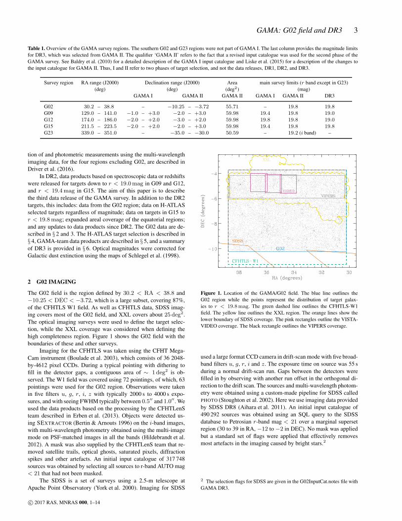
high completeness region. Figure 1 shows the G02 field with the

boundaries of these and other surveys.

Imaging for the CFHTLS was taken using the CFHT Mega-

Cam instrument (Boulade et al. 2003), which consists of 36 2048-

by-4612 pixel CCDs. During a typical pointing with dithering to

fill in the detector gaps, a contiguous area of ∼ 1 deg2 is ob-

served. The W1 field was covered using 72 pointings, of which, 63

pointings were used for the G02 region. Observations were taken

in five filters u, g, r, i, z with typically 2000 s to 4000 s expo-

sures, and with seeing FWHM typically between 0.5′′ and 1.0′′ . We

used the data products based on the processing by the CFHTLenS

team described in Erben et al. (2013). Objects were detected us-

ing SEXTRACTOR (Bertin & Arnouts 1996) on the i-band images,

with multi-wavelength photometry obtained using the multi-image

mode on PSF-matched images in all the bands (Hildebrandt et al.

2012). A mask was also supplied by the CFHTLenS team that re-

moved satellite trails, optical ghosts, saturated pixels, diffraction

spikes and other artefacts. An initial input catalogue of 317 748

sources was obtained by selecting all sources to r-band AUTO mag

< 21 that had not been masked.

The SDSS is a set of surveys using a 2.5-m telescope at

Apache Point Observatory (York et al. 2000). Imaging for SDSS

Figure 1. Location of the GAMA/G02 field. The blue line outlines the

G02 region while the points represent the distribution of target galax-

ies to r < 19.8mag. The green dashed line outlines the CFHTLS-W1

field. The yellow line outlines the XXL region. The orange lines show the

lower boundary of SDSS coverage. The pink rectangles outline the VISTA-

VIDEO coverage. The black rectangle outlines the VIPERS coverage.

used a large format CCD camera in drift-scan mode with five broad-

band filters u, g, r, i and z. The exposure time on source was 55 s

during a normal drift-scan run. Gaps between the detectors were

filled in by observing with another run offset in the orthogonal di-

rection to the drift scan. The sources and multi-wavelength photom-

etry were obtained using a custom-made pipeline for SDSS called

PHOTO (Stoughton et al. 2002). Here we use imaging data provided

by SDSS DR8 (Aihara et al. 2011). An initial input catalogue of

490 292 sources was obtained using an SQL query to the SDSS

database to Petrosian r-band mag < 21 over a marginal superset

region (30 to 39 in RA, −12 to −2 in DEC). No mask was applied

but a standard set of flags were applied that effectively removes

most artefacts in the imaging caused by bright stars.2

2 The selection flags for SDSS are given in the G02InputCat.notes file with

GAMA DR3.

c© 2017 RAS, MNRAS 000, 1–14

4 I.K. Baldry et al.

3 G02 TARGET SELECTION

Targets were selected from both the CFHTLenS and SDSS DR8

input catalogues, described above, which were then merged. SDSS

objects were matched to the nearest CFHTLenS object within a 2′′

matching radius. If an SDSS object did not have a counterpart in the

CFHTLenS catalogue then a new object was added to the merged

catalogue (e.g., this can happen for galaxies that were initially lost

in the large CFHTLenS bright star halos). Objects could be selected

for spectroscopic targeting using photometry from either input cat-

alogue, whether or not they had photometry from one or both.

For the G02 main survey, galaxies with r < 19.8mag af-

ter correction for Galactic dust extinction were targeted in G02.

The type of magnitudes used, for this flux-limited selection, were

SEXTRACTOR AUTO (Kron 1980; Bertin & Arnouts 1996) for

CFHTLenS and Petrosian (Petrosian 1976; Stoughton et al. 2002)

for SDSS. These both use adaptive apertures. Other magnitudes

used were 3′′-aperture (SDSS fibre-size) magnitudes, which help

to exclude artefacts related to the adaptive apertures, PSF magni-

tudes and profile-fitted (PSF+model) magnitudes. The differences

between the latter two magnitudes for each source was used by

SDSS as a star-galaxy profile separator.

Galaxies were targeted if they met the r < 19.8 criterion in

either the CFHTLenS or SDSS input catalogues, with details be-

low:

• For CFHTLenS, the selection criteria were objects with SEX-

TRACTOR CLASS STAR < 0.70 and rauto < 19.8mag. In ad-

dition: targets were required to have an r-band 12 pixel (3′′, i.e.,

SDSS-size fibre) aperture magnitude in the range 17 < rfib <22.5; and data in masked regions were excluded, for example,

around bright stars.

• For SDSS DR8, the selection criteria were galaxies with

rPetro < 19.8mag. Star-galaxy separation for SDSS was done us-

ing the method outlined by Baldry et al. (2010), without the J −Kmeasurements, using a combination of r-band PSF and model mag-

nitudes (Stoughton et al. 2002) as follows:

rpsf−rmodel >0.250.25− 1

15(rmodel − 19)

0.15for

rmodel < 19.019.0 ... 20.5rmodel > 20.5

(1)

SDSS selected targets had an SDSS r-band fibre magnitude in the

range 17 < rfib < 22.5. A number of standard flags were also

applied to exclude artefacts.

Filler targets were selected down to r < 20.2mag (with lower

priority) from both surveys using the same criteria, other than the

change in magnitude limit, outlined above.

Data for the targets are given in the G02TilingCat table. Tar-

gets selected as part of the main survey can be identified using the

G02 survey class (SC) parameter. The SC parameter takes the val-

ues: 6 for main-survey targets selected from SDSS and CFHTLenS;

5, from SDSS only; 4, from CFHTLenS only; and 2 for filler tar-

gets selected from either. Visual classification was performed on a

subset of SC > 4 sources, particularly those with discrepant pho-

tometry between the two input catalogues, to identify artefacts, de-

blended parts of large galaxies and severely affected photometry.

Based on these visual checks, 290 sources were given an SC value

of zero to indicate that they were not a target. The number of re-

maining main survey (SC > 4) targets in G02TilingCat is 59 285.

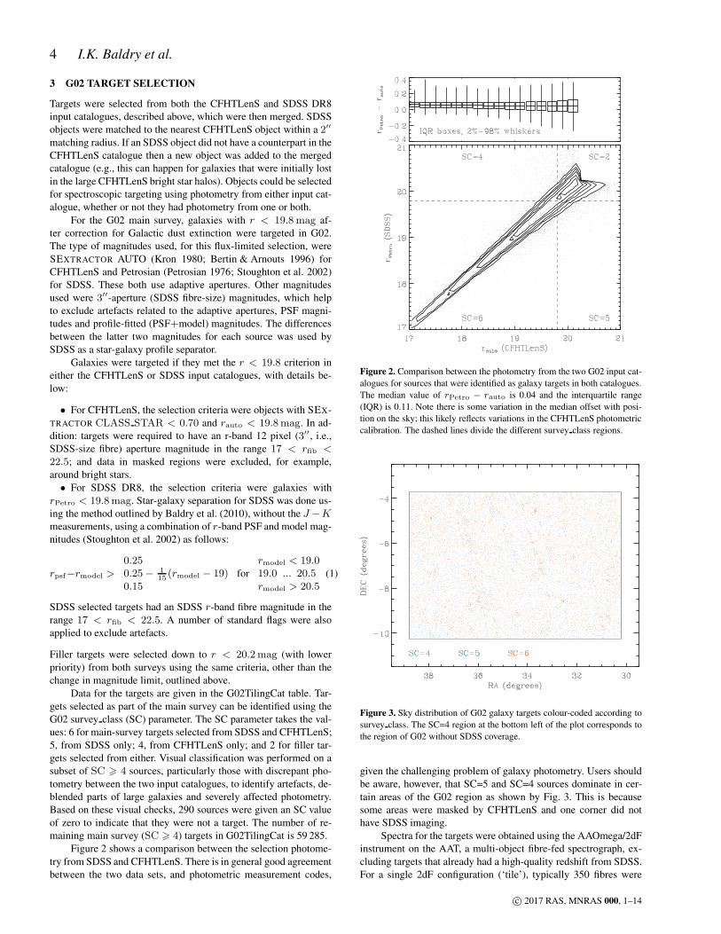
Figure 2 shows a comparison between the selection photome-

try from SDSS and CFHTLenS. There is in general good agreement

between the two data sets, and photometric measurement codes,

Figure 2. Comparison between the photometry from the two G02 input cat-

alogues for sources that were identified as galaxy targets in both catalogues.

The median value of rPetro − rauto is 0.04 and the interquartile range

(IQR) is 0.11. Note there is some variation in the median offset with posi-

tion on the sky; this likely reflects variations in the CFHTLenS photometric

calibration. The dashed lines divide the different survey class regions.

Figure 3. Sky distribution of G02 galaxy targets colour-coded according to

survey class. The SC=4 region at the bottom left of the plot corresponds to

the region of G02 without SDSS coverage.

given the challenging problem of galaxy photometry. Users should

be aware, however, that SC=5 and SC=4 sources dominate in cer-

tain areas of the G02 region as shown by Fig. 3. This is because

some areas were masked by CFHTLenS and one corner did not

have SDSS imaging.

Spectra for the targets were obtained using the AAOmega/2dF

instrument on the AAT, a multi-object fibre-fed spectrograph, ex-

cluding targets that already had a high-quality redshift from SDSS.

For a single 2dF configuration (‘tile’), typically 350 fibres were

c© 2017 RAS, MNRAS 000, 1–14

GAMA: G02 field and DR3 5

allocated to targets and 25 fibres were allocated to positions for de-

termining a mean sky background. The AAOmega dual-beam setup

was chosen so that spectra were obtained from 3750A to 8850A

with a dichroic split at 5700A. The dispersion was 1A per pixel in

the blue arm and 1.6A per pixel in the red arm. For an observa-

tion of a tile, data from usually three exposures and from each arm

were combined such that a single sky-subtracted spectrum per tar-

get was obtained (Hopkins et al. 2013). The redshifts for each spec-

trum were then measured using a robust and reliability-calibrated

cross-correlation method (Baldry et al. 2014).

The tiling strategy was similar to the GAMA equatorial re-

gions (Robotham et al. 2010) with priorities from high-to-low for:

main-survey targets that had not been observed spectroscopically,

main-survey targets with one spectrum but no reliable redshift,

quality-control targets, and filler targets. Clustered main-survey tar-

gets, defined as being within 40′′ of another main-survey target,

were given a boosted priority. This helps with the strategy of ob-

taining high completeness, regardless of target density, with mul-

tiple visits because of the necessity in avoiding fibre collisions on

any single visit.

Note that it became apparent during 2013 that the time allo-

cated for the GAMA survey was not going to allow completion

of the G02 region to a high completeness level. At this stage, it

was decided to prioritise the overlap with the XXL survey. In the

last season of observing, main-survey targets north of −6.0 were

given the highest priority though some targets between −6.3 and

−6.0 were observed to avoid a hard edge in completeness. As a

result of this, the redshift completeness is 95.5% for the main sur-

vey north of −6.0, 46.4% between −6.3 and −6.0, and 31%

south of −6.3, on average. The redshift completeness is defined

as the percentage of objects in a sample with reliable redshifts. Fig-

ure 4 shows a completeness map of the G02 region. Note that for

the area south of −6.0, the completeness is significantly higher

for clustered targets compared to unclustered targets.

It is clear that the 19.5 deg2 area north of −6.0 has the fi-

delity required for a robust group catalogue and other clustering

measurements, however, care must be taken to understand the ef-

fect of combined SDSS and CFHTLenS selection. There are 21 152

main-survey targets, of which 20 200 have a reliable redshift with

nQ > 3 (completeness of 95.5%; nQ is the redshift quality flag

as defined in Liske et al. 2015). The completeness is 96.2% for

main-survey targets that have a CFHTLenS r-band AUTO mag

measurement. Figure 5 shows the magnitude distribution of targets

and the redshift completeness versus rauto. The magnitude distri-

bution is also shown divided according to source of redshift: SDSS

or AAOmega, and in the latter case whether more than one spec-

trum was taken. This demonstrates that in order to obtain high com-

pleteness at the faint end, it is necessary to observe many of the tar-

gets twice. This can compensate for variable conditions and fibre

throughput, as well as allowing coadding of two spectra to increase

the signal-to-noise ratio.

Figure 6 shows the redshift histogram of the GAMA-

G02 high-completeness area. Also shown are the histograms

for VIPERS (Garilli et al. 2014) and PRIMUS (Coil et al. 2011),

which covers part of G02. VIPERS uses photo-z selection to target

galaxies at z > 0.5, thus, there are almost no common targets be-

tween GAMA and VIPERS (which covers ∼ 15 deg2). In consider-

ation of matching with XXL, for example, this leads to the situation

where the structures are well defined by GAMA at z < 0.35 and by

VIPERS at z > 0.5, with a redshift coverage gap. PRIMUS only

fills this over a significantly smaller area. There are also 11 000 red-

Figure 4. Map of the redshift completeness of the G02 field. The colour

coding is according to the percentage of main-survey targets (SC > 4)

with a reliable redshift (nQ > 3) in areas of 0.2 × 0.2. The yellow line

outlines the XXL region.

Figure 5. Magnitude distribution and redshift completeness of the main-

survey targets in the G02 field north of −6.0. The colour coding in the

upper panel shows targets with reliable redshifts from SDSS and AAOmega,

and whether or not more than one spectrum were taken for the GAMA

survey. The main-survey targets to the right of the dashed line were selected

because of their SDSS magnitudes (SC=5, see Fig. 2).

shifts available from VVDS (Le Fevre et al. 2013), not shown, over

about 0.6 deg2 with a redshift interquartile range of 0.54–1.12.

The G02 group catalogue was constructed using the same code

as presented in Robotham et al. (2011), primarily over the highly

complete region of G02 (declination > −6). To make use of the

less complete redshifts available below declination −6, we made

a hard cut at declination > −6.3 but use −6 as the border flag

c© 2017 RAS, MNRAS 000, 1–14

6 I.K. Baldry et al.

Figure 6. Redshift histograms for the G02 area, DEC > −6.0, compar-

ing GAMA (solid line), VIPERS (dashed line) and PRIMUS (dotted line).

The bin spacing is 0.01 in ln(1 + z).

within the group finding code. To be consistent with the GAMA

equatorial regions, we use the SDSS rPetro < 19.8mag selected

targets only (SC > 5). After redshift cuts, this results in 20 029

galaxies available for group finding. The resultant group catalogue

has 2 540 ‘groups’ with two or more members. We compute the

same standard group statistics as per Robotham et al. (2011), with

the same halo mass and group luminosity calibrations.

It is important to note that the number of galaxies linked in

each group, NFOF, does not have a physical meaning because it is

defined using a magnitude-limited sample. Here, we compute the

richness using a density-defining population (DDP) that has Mr <−21mag.3 The richness (N ) is the the number of DDP galaxies in

a group. The absolute magnitude is given by

Mr = rPetro − 5 log(DL/10 pc)− kr + 1.03z , (2)

with k-corrections using KCORRECT (Blanton & Roweis 2007) and

with an evolution factor of 1.03 from the Qe value derived by

Loveday et al. (2015) (table 3 of their paper). Given the spectro-

scopic limit of r < 19.8mag, the DDP galaxies are volume limited

to z < 0.28, though we assume the richness values are reliable to

z < 0.3.

The number of ‘rich’ groups, N > 5, in the high-

completeness G02 region (DEC > −6, 19.5 deg2), and in the red-

shift range 0.1 < z < 0.3, is 98. This gives a number density of

3.0× 10−5 Mpc−3. This is higher than the average for the equato-

rial regions but consistent with cosmic variance. For the equatorial

regions divided into nine 20 deg2 areas, the number density ranges

from 2.1×10−5 Mpc−3 to 3.4×10−5 Mpc−3. Figure 7 shows the

distribution of the G02 rich groups in RA and redshift as a ‘cone

plot’.

The groups and clusters from the XXL bright 100 sample

Pacaud et al. (2016), with L500,MT > 1043erg s−1,4 were matched

to GAMA groups, taking the richest group within 6 arcmin and

800 km/s (between the XXL-designated redshift and median red-

shift of GAMA galaxies in a group). All but two XXL groups at

3 We assume a flat ΛCDM cosmology with H0 = 70 km s−1 Mpc−1

and Ωm,0 = 0.3 for absolute magnitudes and distances.4 L500,MT is the estimate of the X-ray luminosity within a radius within

which the average mass density of the cluster equals 500 times the critical

density of the Universe.

redshifts z < 0.4 were matched to N > 5 GAMA groups. The

locations of XXL bright groups are also shown in Fig. 7. The G02

region can thus be used to determine the optical properties of X-ray

selected groups, or vice versa.

4 H-ATLAS TARGET SELECTION IN THE

EQUATORIAL REGIONS

The H-ATLAS was the largest open time survey completed with

the Herschel Space Observatory (Eales et al. 2010). This survey

observed 600 deg2 of sky including four of the GAMA regions,

with imaging in five bands from 100µm to 500µm. The 4σ limit

at 250µm is about 30 mJy (Valiante et al. 2016). The FWHM of

the PSF is about 18′′ , which is significantly larger than the opti-

cal images. One technique developed to identify counterparts was

a likelihood-ratio technique that assigns a reliability R to nearby

SDSS sources (Smith et al. 2011).

The H-ATLAS chose the GAMA equatorial regions in order

to increase the number of available redshifts matched to H-ATLAS

sources compared to, for example, SDSS or 2dFGRS. This is be-

cause of the higher median redshift of GAMA compared to the

shallower redshift surveys. The GAMA main survey in the equa-

torial regions is primarily rPetro < 19.8mag but also includes

about 2000 targets from z-band and K-band selection (Baldry et al.

2010). In February 2011, L. Dunne provided the GAMA team

with a preliminary cross-identification of H-ATLAS sources with

SDSS imaging based on the method of Smith et al. (2011). Any

matches (reliability R > 0.8), that were not in the GAMA main

survey, were included as AAOmega filler targets if they satisfied

rmodel < 20.6mag, passed the GAMA star-galaxy separation and

were not in masked regions.

The observations of the GAMA equatorial regions with

AAOmega went well such that nearly all of the main survey tar-

gets had a spectrum taken, and this meant that 86% of H-ATLAS

filler targets had a spectrum taken as well. This happened because,

toward the end of the observations, we could not fill every tile with

main survey targets that either did not have a reliable redshift mea-

surement or were not already observed twice.

Subsequent to the selection of filler targets in 2011, the

H-ATLAS team had obtained some additional Herschel imag-

ing, improved reductions, and improved the cross-identification.

The cross-identifications with SDSS are described in Bourne et al.

(2016). Thus, the identifications that are given in the H-ATLAS

data release are not the same as used for the GAMA filler targets.

An assessment of the completeness issues associated with using the

H-ATLAS data release and GAMA redshifts is described below.

We selected an H-ATLAS-GAMA sample as follows.5 The

H-ATLAS optical identifications were matched to the GAMA in-

put catalogue, and the tiling catalogue that contains redshift infor-

mation. Sources were selected that: were in the GAMA equato-

rial regions, passed the r-band star-galaxy separation (Eq. 1), had

rmodel < 20.6mag, were not masked by GAMA, had H-ATLAS-

SDSS cross-matching reliability R > 0.8, and had m250 <12.72mag (AB magnitudes from best flux estimate in the 250-

µm band; flux density > 29.65mJy). The completeness of H-

ATLAS detections is significantly lower at fainter 250-µm mag-

nitudes (Valiante et al. 2016).

5 We used the data table HATLAS DR1 CATALOGUE V1.2 from

http://www.h-atlas.org/public-data/download

c© 2017 RAS, MNRAS 000, 1–14

GAMA: G02 field and DR3 7

Figure 7. Cone plot of the GAMA groups in the G02 high-completeness region (−6.0 < DEC < −3.72, the two dimensions shown correspond to RA and

redshift). The GAMA groups with richness N > 5 are shown with filled circles, shaded according to the number of galaxies with Mr < −21mag. The XXL

clusters from the bright cluster sample of Pacaud et al. (2016) are shown with red circles.

Figure 8. H-ATLAS selected galaxies in the GAMA regions with 20.0 < rmodel < 20.6. The black points represent sources that were not GAMA targets,

while the orange points represent sources that were GAMA targets. The blue solid lines outline the areas where there was H-ATLAS coverage prior to February

2011, and therefore H-ATLAS selection was available for the GAMA filler sample. Saw-tooth boundaries are limits of the H-ATLAS coverage arising from

Herschel observing constraints.

Figure 8 shows the distribution of these H-ATLAS selected

galaxies with rmodel > 20mag. Also shown is whether or not they

were a GAMA target. This demonstrates that the Herschel imag-

ing over half of G12 was not available for filler selection in 2011.

Only the targets that were within the blue solid outlines shown on

Fig. 8 were selected for this reason. This left an H-ATLAS-GAMA

sample of 20 380 sources.

Figure 9 shows a histogram of the sample in rmodel, with

colour filling where there are reliable redshifts. The redshift com-

pleteness is high for rmodel < 19.6mag but drops off at fainter

magnitudes (this would be a sharp drop at 19.8 in rPetro because of

the GAMA main survey selection). Figure 10 shows how the com-

pleteness depends on m250 and rmodel. This makes it clear there

is a region of low completeness at faint magnitudes in both filters.

This can be understood in terms of separate effects associated with

targeting completeness and redshift success rate.

Targeting completeness is defined as the percentage of ob-

jects in a sample that have been observed spectroscopically. This

is essentially 100% for targets that are in the main survey (15 453),

but depends on m250 for non-main survey targets (4 927) as shown

in Fig. 11. From this, it is clear that the targeting completeness is

high for m250 < 12.35mag and drops off significantly at fainter

magnitudes. This reflects the change in the cross-identifications

between GAMA filler selection and the H-ATLAS data release

(Bourne et al. 2016).

The other feature of the redshift completeness map shown in

Fig. 10 is the drop off toward fainter rmodel. This is caused by a

decrease in the redshift success rate, which is defined as the per-

centage of spectroscopically-observed targets that have a reliable

redshift measurement, as shown in Fig. 12. To summarize, the red-

shift completeness map of the H-ATLAS-GAMA sample in Fig. 10

can be explained in terms of: 100% targeting completeness for main

survey sources; about 75% targeting completeness for non-main

survey sources at m250 < 12.35mag with a drop off fainter than

this; and for all sources, a general decrease in redshift success rate

with rmodel fainter than 19.5.

To show the demographics of the H-ATLAS-GAMA sample,

we select sources with galaxy spectroscopic redshifts less than 0.8,

m250 < 12.35mag, a random selection of 75% of the main survey,

and all the fillers to rmodel < 20.6mag. This is unbiased within

these magnitude limits other than the redshift success rate variation

(Fig. 12). The distribution of this sample in visible-band absolute

magnitude versus redshift is shown in Fig. 13, with colour cod-

ing according to far-IR luminosity. This clearly demonstrates the

increase in the number density of the most luminous far-IR galax-

ies (L250 > 1025WHz−1; cf. Dye et al. 2010; Guo et al. 2014).

The filler sample is particularly useful for selecting luminous far-

IR galaxies at 0.4 < z < 0.8.

c© 2017 RAS, MNRAS 000, 1–14

8 I.K. Baldry et al.

Figure 9. Histogram showing sources of redshifts to the H-ATLAS matched

sample as a function of magnitude. The solid line shows the H-ATLAS-

GAMA selected sample described in the text. The dotted line shows sources

that either have a reliable redshift or were a GAMA target. The coloured

filling is according to source of redshift.

Figure 10. Redshift completeness of the H-ATLAS-GAMA sample as a

function of 250-µm magnitude and rmodel. The colour scale representing

completeness percentage is the same as in Fig. 4.

Figure 11. Targeting completeness for the H-ATLAS-GAMA sample as a

function of m250 . The solid and dashed line show the completeness for non-

main survey and main survey sources. The dotted line shows the fraction of

the non-main survey sources that were assigned as filler targets in February

2011.

Figure 12. Redshift success rate as a function of rmodel for the H-ATLAS-

GAMA sample.

Figure 13. Demographics of the H-ATLAS-GAMA sample to rmodel <

20.6mag and m250 < 12.35mag with spectroscopic redshifts. The

dashed line shows the r-band magnitude limit using an average k-correction

as a function of redshift. The points are colour coded according to their 250-

µm rest-frame luminosity, which is estimated using m250 and an average

k-correction as a function of redshift.

5 DATA MANAGEMENT UNITS

The GAMA database is organised into data management units

(DMUs). Here they are briefly introduced with any significant up-

dates noted.

5.1 Spectroscopic, redshift and input catalogue DMUs

5.1.1 SpecCat

This DMU includes the spectra and redshifts obtained from the

AAT, and tables combining the redshifts from all the curated spec-

troscopic data for the GAMA survey. In DR2, the redshifts from

AAT spectra were obtained using the semi-automatic code RUNZ

(Saunders, Cannon, & Sutherland 2004) with user interaction. For

DR3, the primary choice of redshift has been updated; these are

now from the automatic code AUTOZ (Baldry et al. 2014) except

for some broadlined-AGN spectra.

A detailed description of the redshift procedure using RUNZ,

and other spectroscopic survey procedures, are given in § 2 of

c© 2017 RAS, MNRAS 000, 1–14

GAMA: G02 field and DR3 9

Liske et al. (2015), while the AUTOZ method and its calibration are

described in detail in Baldry et al. (2014). An analysis of the survey

redshift completeness, and a comparison between redshift accuracy

from AUTOZ and RUNZ, are described in § 3 of Liske et al. (2015).

5.1.2 ExternalSpec

Spectra and redshifts were curated from 10 other surveys within

the GAMA regions. These external spectroscopic surveys are used

for 12% of the best redshifts of the main-survey targets (equatorial

and G02 regions). This DMU is described in § 2.7 of Liske et al.

(2015), and the list of surveys is given in table 2 of that paper.

5.1.3 EqInputCat

This DMU includes the input catalogue and the tiling catalogue for

GAMA equatorial regions, G09, G12 and G15. The input catalogue

was derived from SDSS. Previous versions of the tiling catalogue

were used to track redshift completeness during the observations.

The current version is designed to be used as a starting point for

selecting well defined samples, from the best redshifts for each

source and information on target selection. Visual classifications

were made for a significant fraction of sources in order to identify

deblends and artefacts.

A detailed description of the procedure for defining the input

catalogue and selecting targets is given in Baldry et al. (2010). Up-

dates to the DMU are described in § 2.9 of Driver et al. (2011) and

§ 2.1 of Liske et al. (2015).

5.1.4 G02InputCat

The input catalogue and tiling catalogue for the G02 region are

described in § 2 and § 3 of this paper.

5.1.5 SpecLineSFR

This DMU contains three tables with line flux and equivalent

width measurements for GAMA II spectra, which have nQ > 1and 0.002 < z < 1.35. As well as providing the additional

measurements for the G02 region, there are several key differ-

ences between this DMU version and an earlier version used in

DR2 (Gunawardhana et al. 2013, Hopkins et al. 2013, § 5.1.10 of

Liske et al. 2015). First, this DMU provides line fluxes and equiv-

alent widths (EWs) measured in a consistent manner for spectra

from several surveys that used AAOmega, SDSS, 2dF or 6dF; al-

though we note that flux measurements are only useful for the

SDSS and AAOmega spectra that were flux calibrated. Second, un-

certainties are estimated for the line flux and EWs by propagat-

ing the formal uncertainties on the fitted parameters. Third, we in-

clude direct summation EW measurements for various line species,

as well as estimates of the strength of the 4000A break, D4000.

Fourth, we include more complicated two-Gaussian fits to the Hαand Hβ emission lines where the second component accounts for

broad emission or stellar absorption. We include various model se-

lection techniques to determine where more complicated models

are favoured over simple ones. The fitting, line measurements and

model selection techniques are described in detail in Gordon et al.

(2017).

5.1.6 LocalFlowCorrection

This DMU provides corrections from the heliocentric redshifts to

the cosmic-microwave-background frame, and uses the flow model

of Tonry et al. (2000) to provide redshifts primarily corrected for

Virgo-cluster infall at low redshift. The procedure for, and the effect

of, this are described in detail in § 2.3 of Baldry et al. (2012).

5.2 Image analysis DMUs

5.2.1 ApMatchedPhotom

This DMU provides AUTO (Kron) and Petrosian photometry, as

well as other SEXTRACTOR outputs (Bertin & Arnouts 1996) for

the ugrizZY JHK bands. The DMU is described in detail in

Driver et al. (2016). This outlines the processing of the VISTA

VIKING data (Sutherland 2012; Edge et al. 2013) in detail, along

with aperture-matched photometry from SDSS ugriz and VISTA

ZY JHK. As part of the process all data were smoothed to a com-

mon seeing FWHM of 2′′ to ensure accurate colour measurements.

Earlier versions of ApMatchedPhotom were based on SDSS and

UKIDSS (Warren et al. 2007)) data and later versions on SDSS and

VISTA VIKING data where a significant improvement was seen in

the near-IR colours in particular. ApMatchedPhotom has been su-

perseded by the in-house LAMBDAR code (Wright et al. 2016) but

is included in this release for completeness and verification of ear-

lier publications.

5.2.2 SersicPhotometry

The Sersic Photometry DMU provides single-component Sersic

(1968) fit results for sources across the GAMA equatorial survey

regions. Independent fits are provided for each galaxy in each of

the SDSS ugriz, UKIDSS Y JHK and VISTA ZY JHK pass-

bands. Galaxy models are constructed using SIGMA v1.0-2 (Struc-

tural Investigation of Galaxies via Model Analysis, Kelvin et al.

2012). SIGMA is a wrapper around several contemporary astron-

omy tools including Source Extractor (Bertin & Arnouts 1996),

PSF Extractor (Bertin 2011) and GALFIT 3 (Peng et al. 2010), as

well as analysis and processing code written in the open-source R

programming language. In addition to standard GALFIT outputs,

several additional value-added parameters are also output, such as

truncated Sersic magnitudes and central surface brightnesses. Fur-

ther details on the fitting process and outputs may be found in

Kelvin et al. (2012).

5.2.3 GalexPhotometry

This DMU contains catalogues for the NUV and FUV fluxes of

each GAMA galaxy derived using three different methods. These

are ‘simple match photometry’ (nearest neighbour), ‘advanced

match photometry’ and ‘curve-of-growth (CoG) photometry’. In

the second case, UV flux from the GALEX sources is distributed

among the GAMA objects based on knowledge of the positions

and sizes of the objects involved. In the CoG case, surface photom-

etry is performed on the GALEX images at the optically-defined

location of each GAMA galaxy, The procedures are extensively de-

scribed in § 4.2 of Liske et al. (2015).

c© 2017 RAS, MNRAS 000, 1–14

10 I.K. Baldry et al.

5.2.4 WISEPhotometry

This DMU provides the photometry from imaging with the Wide-

field Infrared Survey Explorer for GAMA sources. The con-

struction of the catalogue follows the methodology described in

Cluver et al. (2014), in particular identifying and measuring re-

solved sources. Photometry of GAMA galaxies not resolved by

WISE is taken from the AllWISE Catalogue; here the “stan-

dard aperture” photometry (w*mag) is used, and not the profile-

fit photometry (w*mpro). This is to account for the sensitiv-

ity of WISE when observing extended, but unresolved sources

(Driver et al. 2016). Further details can be found in Jarrett et al.

(2017). All photometry in the DMU has been corrected to re-

flect the updated characterisation of the W4 filter as described in

Brown, Jarrett, & Cluver (2014).

5.2.5 LambdarPhotometry

This DMU provides far-UV to far-IR aperture-matched photome-

try in 21-bands, measured consistently using the Lambda Adaptive

Multi-Band Deblending Algorithm in R (LAMBDAR; Wright et al.

2016). Photometry has been measured using apertures defined as

described in Wright et al. (2016), where a considerable effort has

been made to clean the input catalogue of apertures affected by

contamination or extraction problems such as shredding. Addition-

ally, the photometry is deblended from both GAMA sources and

catalogued contaminants, which are defined independently for the

far-UV to near-IR data, the mid-IR data, and the far-IR data. Fluxes

from this DMU show considerable improvement in panchromatic

consistency, i.e. smoothly changing behaviour with wavelength,

when compared to the catalogue-matched photometry presented in

Driver et al. (2016).

5.2.6 VisualMorphology

This catalogue provides a number of visual morphological classifi-

cations performed for various samples of galaxies in the equatorial

survey regions. In total, 38 795 sources have one or more classifi-

cations.

• A basic visual classification using giH images (SDSS and

UKIDSS/VIKING) was made by 2 team members for sources with

0.002 < z < 0.1. The classes used were: Elliptical, NotElliptical,

Little Blue Spheroid (LBS), Star, Artefact and Uncertain. A earlier

version of the classification was used in Driver et al. (2012).

• Hubble type galaxy classifications were made by 6 team mem-

bers for sources with 0.002 < z < 0.06. These were made using

a decision tree, which was translated to the following classes: E,

S0-Sa, SB0-SBa, Sab-Scd, SBab-SBcd, Sd-Irr, LBS, Star, Artefact.

See § 3 of Kelvin et al. (2014) and § 3.1 of Moffett et al. (2016) for

details.

• Disturbed galaxy classifications were made by 24 team mem-

bers with multiple inspections of galaxies in close pairs and a con-

trol sample, over a redshift range of 0.01–0.33 depending on stellar

mass. Inspections were made of inverted grK images of 60 kpc

× 60 kpc around each source using SDSS and VIKING data. The

classes used were: Disturbed, Normal, and Unsure. See § 2.5 of

Robotham et al. (2014) for details.

• A positional match was made to Galaxy Zoo 1 data

(Lintott et al. 2011) for galaxies with 0.002 < z <0.1. The columns included in this DMU are: P EL, P CS,

P EL DEBIASED, P CS DEBIASED. The first two give the raw

fraction of Galaxy Zoo votes for Elliptical and NotElliptical, re-

spectively, with the second two giving the values corrected for red-

shift bias. See Lintott et al. (2011) for details.

5.3 Spectral energy distribution DMUs

These DMUs make use of photometric measurements and redshifts

to derive rest-frame luminosities, stellar population and dust prop-

erties.

5.3.1 kCorrections

K-corrections are provided in the GALEX FUV and NUV bands,

the SDSS ugriz bands and the UKIDSS Y JHK bands for all

galaxies with redshifts in the GAMA equatorial survey regions

(i.e. excluding G02). As well as the k-corrections themselves, we

provide fourth-order polynomial fits to K(z), the k-correction as

a function of redshift, to aid in the calculation of Vmax values.

These k-corrections are calculated using the eigentemplate fitting

code KCORRECT v4 2 of Blanton & Roweis (2007), and are fur-

ther described in Loveday et al. (2012).

New for DR3, is that we provide k-corrections in passbands

blueshifted by z0 = 0.2 as well as 0.1 and 0.0. The advantage of

using k-corrections for blueshifted passbands is that the uncertain-

ties in the rest-frame magnitudes are smaller when the choice of

bandpass shift is similar to the typical redshifts of a galaxy sam-

ple (cf. Fig. 13). We also provide k-corrections from fits to GAMA

AUTO magnitudes (§ 5.2.1), in addition to those from SDSS model

magnitudes. See § 2 of Loveday et al. (2015) for a discussion of the

advantages of using GAMA AUTO magnitudes for this purpose.

5.3.2 StellarMasses

The StellarMasses DMU comprises estimates of total stellar mass

and other population parameters (including mean stellar age,

dust attenuation, etc.) based on stellar population synthesis (SPS)

of the optical-to-near infrared SEDs. The fits are based on the

Bruzual & Charlot (2003) simple stellar population models, as-

suming a Chabrier (2003) IMF, uniform metallicity, exponentially-

declining star formation histories, and single-screen Calzetti et al.

(2000) dust. The parameter estimation is done in a Bayesian way

(rather than, for example, naive maximum likelihood), which has

an important systematic effect on the inferred values for mass and

mass-to-light ratio (M/L). The main reference for this DMU is

Taylor et al. (2011).

The main improvement in the current version of this catalogue

in comparison to DR2 is the incorporation of the VISTA-VIKING

near-IR photometry, which largely removes the problems seen in

Taylor et al. (2011) when using the UKIDSS near-IR data. In the

fitting, the full ugrizZY JHK SEDs are weighted in such a way

that the fits are to a fixed restframe wavelength range of 3000-

11000 A; i.e. restframe u-Y . This decision is designed to protect

against redshift-dependent biases arising from, for example, the

different availabilities of restframe near-UV information for galax-

ies at different wavelengths. In practice, there are not significant

redshift-dependent systematic differences between the current ver-

sion of the StellarMasses DMU and earlier iterations.

Taylor et al. (2011) have shown that the numerical values of

the SED-fit mass estimates can be approximated using the simple

prescription (solar units): log(M∗/Li) = −0.68+ 0.70(g− i)restwith a typical 1-sigma uncertainty of ∼ 0.12 dex. This provides

c© 2017 RAS, MNRAS 000, 1–14

GAMA: G02 field and DR3 11

authors with a simple way of deriving robust mass estimates from

minimal information. Further, this provides a transparent way for

authors to compare directly to the GAMA mass scale, in order to

identify or account for possible systematic biases in the derivation

of stellar mass estimates. Figure 14 (left) shows M/L versus ob-

served g− i. There is still a tight correlation becoming less steep at

higher redshift. Stellar mass derived using observed g and i mag-

nitudes was used by Bryant et al. (2015) (their eq. 3) for a trans-

parent stellar-mass selection avoiding the need for even SED-fit k-

corrections.

Figure 14 (right) shows M/L in the i-band versus stellar mass

for four redshift slices. This demonstrates the typical range in fitted

M/L is from 0.2 to 2. At higher redshifts, GAMA samples becomes

increasingly biased toward lower M/L because of the r-band mag-

nitude selection limit. In order to create volume- and stellar-mass

limited samples, one needs to select the unbiased region in M/L as

demonstrated by the vertical lines in the figure. These limits were

obtained using a method similar to Lange et al. (2015), see their

fig. 1. Basically one needs to ensure that galaxies of every type

(star-formation history, dust, profile), given a lower stellar-mass

limit, could be selected over the redshift range of the sample. In

practice, it is not always necessary to be quite so strict and one

could relax the stellar-mass limits shown by ∼ 0.1 dex.

5.3.3 MagPhys

The MagPhys DMU is based on parsing the extinction-corrected

flux and flux error for colours from LAMBDAR through MAGPHYS

(da Cunha et al. 2008). The code fits stellar and dust-emission tem-

plates to photometry, with dust attenuation applied to the stellar

templates such that there is a balance between the attenuated and

the dust-emitted energy. Energy balance is correct on average for

a random distribution of galaxy inclinations, but will overestimate

(underestimate) attenuation for face-on (edge-on) disks because of

anisotropic attenuation. The MagPhys DMU provides estimates of

a number of key parameters in particular the stellar mass, dust

mass, and star-formation rate (SFR), which we consider reliable

and useful for broader science. The DMU is described in detail in

Driver et al. (2017).

This DMU provides stellar mass estimates in addition

to the StellarMasses DMU (Taylor et al. 2011). Both use

Bruzual & Charlot (2003) models for the stellar population synthe-

sis and assume a Chabrier (2003) IMF. For the MagPhys DMU,

the dust attenuation uses the Charlot & Fall (2000) model with ab-

sorption redistributed in wavelength assuming various dust compo-

nents for dense stellar birth clouds and for the ambient inter-stellar

medium (da Cunha et al. 2008). Fits are performed to the 21-band

LAMBDAR photometry using models with a range of exponentially-

declining star-formation histories, with bursts, and a range of dust

attenuation. Note however that that the key flux at 250µm is only

measured with a S/N > 2 for about 30% of galaxies. Figure 14

(left) shows a comparison of the M/L, for the different stellar mass

estimates, as a function of observed g − i. The median logarithmic

offset varies from −0.09 for the lowest redshift slice, to −0.03 for

the highest redshift slice shown. The good agreement between the

stellar mass estimates demonstrates that the choice of dust attenua-

tion approach does not make a significant difference.

The long-wavelength baseline (UV to far-IR) used by the

MagPhys DMU also allow an estimate of SFR averaged over

timescales less than a Gyr. MagPhys calculates SFRs from a com-

bined UV and total IR SED fit, summing both the unobscured and

obscured star formation, and provides various estimates over differ-

Figure 14. Mass-to-light ratios for four redshift slices versus observed

colour (left) and stellar mass (right). Solar units are used for M/L and stel-

lar mass. The red contours and points show stellar masses from the Stel-

larMasses DMU (Taylor et al. 2011) while the black contours show the

MagPhys DMU (Driver et al. 2017). The vertical dashed lines represent the

lower limits in stellar mass for unbiased, volume-limited, samples for the

four different redshift limits. Note the stellar masses use LAMBDAR pho-

tometry whereas the samples are selected to rPetro < 19.8mag.

ent timescales. For estimates of the SFR over the last 0.1 Gyr, the

formal 1-sigma errors typically range from 0.2 dex to 0.6 dex.6 De-

tailed comparisons between these MagPhys SFRs and other SFR

indicators in GAMA are discussed in Davies et al. (2016, 2017),

and are used to determine the cosmic star-formation history in

Driver et al. (2017).

5.4 Environment DMUs

5.4.1 GroupFinding

This DMU provides the GAMA Galaxy Group Catalogue (G3C)

for the GAMA equatorial and G02 survey regions. The G3C is one

of the major data products for the GAMA project. At the most basic

level it is a friends-of-friends (FoF) group catalogue that has been

run on GAMA survey style mocks to test the quality of the grouping

6 The median estimate of the logarithm of the SFR over the last 108 yr

is given by the column sfr18 percentile50 for each galaxy in the Mag-

Phys DMU. An estimate of the 1-sigma error was determined using

(sfr18 percentile84 − sfr18 percentile16)/2. This encomposes measure-

ment and fitting errors.

c© 2017 RAS, MNRAS 000, 1–14

12 I.K. Baldry et al.

and then run on the real GAMA data in order to extract our best

effort groups. The details of the process are discussed extensively

by Robotham et al. (2011).

There have been a number of minor changes since the first ver-

sion used by the GAMA team. Redshifts now use the CMB frame

instead of the heliocentric frame. We include galaxies with lower-

quality nQ = 2 redshifts (AUTOZ calibrated probability of 0.4 to

0.9) because if these galaxies link with a group, they are likely at

the correct redshift since the chance of accidentally being aligned

with a group is small. The grouping parameters were re-calibrated

over a larger suite of GAMA mock lightcones (Farrow et al. 2015)

created using the Gonzalez-Perez et al. (2014) model.7

The parameters are b0 = 0.0608, R0 = 18.5000, Eb =0.0449, Er = −0.0712, and ν = 0.7830 as defined in § 2.1 of

Robotham et al. (2011). These determine the linking length in the

radial and line-of-sight directions as a function of survey location.

The impact of these new grouping parameters is ultimately

very small, with grouping changes at the ∼ 1% level. A bigger up-

date has been to use the Farrow et al. (2015) randoms catalogue to

determine the global redshift volume density [n(z)] rather than the

luminosity function fit originally used in Robotham et al. (2011).

Out to redshift z = 0.3, the difference between the two methods

for estimating the local density of observable points is small, but at

higher redshifts they smoothly diverge at the 10% level, resulting

in larger implied densities and smaller implied FoF links. The im-

pact of this change is still fairly minor, but it does result in fewer

grouped high-redshift galaxies.

5.4.2 FilamentFinding

Elements of large-scale structure are clearly visible in GAMA data.

The FilamentFinding DMU identifies and characterizes filaments

and voids using a multiple-pass modified minimum spanning tree

(MST) algorithm. Initially, group centres from the GroupFinding

DMU are used as nodes for a MST that identifies filaments. All

galaxies within a distance r of each filament are said to be filament

galaxies associated with that structure. A second MST is gener-

ated from all galaxies that are not associated with filaments; this

identifies smaller-scale interstitial structures dubbed as ‘tendrils’

(Alpaslan et al. 2014a), which typically contain few galaxies and

exist within underdense regions. Galaxies that are beyond a dis-

tance q from a tendril are said to be isolated void galaxies. r and qare selected so as to minimize the volume-weighted two point cor-

relation function of the void galaxy population. For further details,

see Alpaslan et al. (2014a,b).

5.4.3 GeometricEnvironments

This DMU identifies the cosmic web of large scale structure within

the GAMA equatorial survey regions by classifying the geometric

environment of each point in space as either a void, a sheet, a fil-

ament or a knot. The classification system is based on evaluation

of the deformation tensor (i.e. the Hessian of the gravitational po-

tential) on a grid. The number of eigenvalues above an imposed

7 The GAMA lightcone mocks are available through the Virgo database

portal at virgodb.dur.ac.uk (GAMA v1 table). They are built on the Millen-

nium MR7 dark-matter-only simulation (Guo et al. 2013) and are populated

with galaxies following the Gonzalez-Perez et al. (2014), and an early ver-

sion of the Lacey et al. (2016), semi-analytic galaxy formation models.

threshold indicates the number of collapsed dimensions of struc-

ture at that location – either 0, 1, 2 or 3, corresponding to a void,

sheet, filament or knot, respectively. The classification of the grid,

as given in the GeometricGrid table, allows the geometric environ-

ment of any object within the grid (any object in the G09, G12 or

G15 regions with 0.04 < z < 0.263) to be determined by assign-

ing the object the same environment as the cell of the grid in which

the object is located. See Eardley et al. (2015) for full details of the

DMU.

5.4.4 EnvironmentMeasures

The EnvironmentMeasures DMU provides three different metrics

of the local environment of GAMA galaxies. The three different

metrics are the 5th nearest-neighbour surface density (Brough et al.

2013), the number of galaxies within a cylinder (Liske et al. 2015),

and the adaptive Gaussian environment parameter (Yoon et al.

2008). The method used to calculate these has not changed from

DR2 to DR3.

5.4.5 Randoms

The random catalogue DMU contains a series of randomly-placed

points (‘randoms’), each tagged with a galaxy CATAID, that fill the

volume of the equatorial fields of the GAMA survey in a way that

follows the galaxy selection-function. It is designed to be used as

a reference for measuring overdensities and estimating clustering

statistics. See Farrow et al. (2015) for details.

The method used to produce these points was introduced in

Cole (2011), whilst the particular implementation for GAMA is

given in Farrow et al. (2015). The method involves cloning real

galaxies, with each random point in the catalogue being stored with

the CATAID of its parent. This allows the randoms to be assigned

galaxy properties by matching on CATAID. Once properties are as-

signed to the randoms a suitable random catalogue can be produced

by applying the same sample selection cuts as applied to the galax-

ies. One must, however, take care when using luminosity-selected

samples, as a particular form of luminosity evolution is explicitly

assumed in their production. In addition, if your sample has addi-

tional sources of incompleteness beyond the r < 19.8 selection,

for example a Hα flux limit, further work is required so please con-

tact the DMU authors (for an example of this, see Gunawardhana

et al. in preparation).

The DMU contains two tables. In RANDOMSUNWINDOWED

the standard Cole (2011) method is used, whilst in the RAN-

DOMS table the randoms created from a cloned galaxy are re-

stricted to a window around the redshift of that galaxy, as explained

in Farrow et al. (2015). The window is designed to minimise the

impact of any unmodeled galaxy evolution effects on the random

n(z).

The DMU version of the randoms has two important differ-

ences to the ones used in Farrow et al. (2015). Firstly, the parame-

ters used to model luminosity evolution have been changed follow-

ing the results of Loveday et al. (2015). Secondly the size of the

redshift window has been increased, to adjust the balance between

limiting the effect of unmodeled galaxy-evolution and keeping the

window large enough to completely remove large-scale structure

from the input catalogue.

c© 2017 RAS, MNRAS 000, 1–14

GAMA: G02 field and DR3 13

6 DATA RELEASE 3

The third GAMA data release (DR3) provides AAT/AAOmega

spectra, redshifts and a wealth of ancillary information for pri-

marily 215 260 objects from the GAMA II survey (Table 1). Of

these, 178 856 are main survey objects and 36 404 are fillers. In

turn, 150 465 (84%) and 4 344 (12%) of these, respectively, have

secure redshifts. DR3 updates all data previously released in DR2,

and significantly expands on DR2: DR3 includes both more ob-

jects and a wider range of data products than DR2. DR3 thus

supersedes DR2 in every way. The data release is available at

http://www.gama-survey.org/dr3/∼.

In DR3 we are releasing data primarily for the following

GAMA II objects:

• Main survey objects: all for G02 and G15, r < 19.0magselected for G09 and G12;

• Fillers: all for G02, H-ATLAS selected for G09, G12 and G15.

The region areas and main survey limits for GAMA I, GAMA II

and DR3 are shown in Table 1. In addition, we include a small set

of objects that were part of DR2 or the H-ATLAS DR1 and not

already covered by the selection above. Note that for G02, we are

releasing all GAMA II data, and for G15, all main survey data. The

environment measurements that use the equatorial main survey are

only available for G15.

GAMA DR3 doubles the number of galaxies with released

spectroscopic redshifts compared to DR2 (Liske et al. 2015). New

redshifts are available, in particular, for the G02 region (§ 3), H-

ATLAS selected sources (§ 4), and in G15. The redshift measure-

ments now use the more accurate AUTOZ code (Baldry et al. 2014).

New environment measurements for G15 are made available in-

cluding a filament catalogue (Alpaslan et al. 2014a), and geomet-

ric measurements (Eardley et al. 2015). The galaxy distribution is

shown in Fig. 15 with colour coding to showcase the different en-

vironment classifications. New image analysis is made available

including LAMBDAR photometry (Wright et al. 2016) that provides

consistent photometry across all the bands from the far-UV to far-

IR. All the available redshifts, including the G23 region, and all

GAMA data products will be made available in DR4.

ACKNOWLEDGEMENTS

GAMA is a joint European-Australasian project based around a

spectroscopic campaign using the Anglo-Australian Telescope. The

GAMA input catalogue is based on data taken from the Sloan Digi-

tal Sky Survey and the UKIRT Infrared Deep Sky Survey. Comple-

mentary imaging of the GAMA regions is being obtained by a num-

ber of independent survey programmes including GALEX MIS,

VST KiDS, VISTA VIKING, WISE, Herschel-ATLAS, GMRT and

ASKAP providing UV to radio coverage. GAMA is funded by the

STFC (UK), the ARC (Australia), the AAO, and the participating

institutions. The GAMA website is http://www.gama-survey.org/ .

I. Baldry acknowledges funding from Science and Technology

Facilities Council (STFC) and Higher Education Funding Coun-

cil for England (HEFCE). L. Dunne acknowledges support from

the European Research Council advanced grant COSMICISM and

also consolidator grant CosmicDust. H. Hildebrandt is supported

by an Emmy Noether grant (No. Hi 1495/2-1) of the Deutsche

Forschungsgemeinschaft. P. Norberg acknowledges the support of

the Royal Society through the award of a University Research Fel-

lowship, and of the Science and Technology Facilities Council

(ST/L00075X/1).

Figure 15. Galaxy distribution in the GAMA G15 field showing different

environmental measurements. Galaxies were selected with 0.10 < z <

0.18 and −1.5 < dec < 1.5 (the two dimensions shown correspond

to RA and redshift). Each panel shows the galaxies colour coded according

to environment: top panel, using the 5th nearest neighbour surface density

(Brough et al. 2013); middle panel, using the geometric environment classi-

fications (Eardley et al. 2015); lower panel, using the filament-finder classi-

fications (Alpaslan et al. 2014a). The top two panels show a volume-limited

sample with Mr < −20.0mag, while the filament finder uses only galax-

ies with Mr < −20.55mag (h = 0.7). In the latter case, the classified

groups, from the FoF catalogue (Robotham et al. 2011), used as the starting

point of the filament finder, are those with two or more members from the

volume-limited sample. Also shown are rich groups shaded according to the

number of member galaxies with Mr < −21.0mag (cf. Fig. 7). Note also

the FilamentFinding DMU provides links beween galaxies and groups in a

filament.

REFERENCES

Aihara H., et al., 2011, ApJS, 193, 29

Alpaslan M. et al., 2014a, MNRAS, 438, 177

Alpaslan M. et al., 2014b, MNRAS, 440, L106

Baldry I. K. et al., 2014, MNRAS, 441, 2440

Baldry I. K. et al., 2012, MNRAS, 421, 621

Baldry I. K. et al., 2010, MNRAS, 404, 86

Bertin E., 2011, in ASP Conf. Ser. 442, Astronomical Data Anal-

ysis Software and Systems XX, Evans I. N., Accomazzi A.,

Mink D. J., Rots A. H., eds., ASP, San Francisco, p. 435

c© 2017 RAS, MNRAS 000, 1–14

14 I.K. Baldry et al.

Bertin E., Arnouts S., 1996, A&AS, 117, 393

Blanton M. R., Roweis S., 2007, AJ, 133, 734

Boulade O. et al., 2003, Proc. SPIE, 4841, 72

Bourne N. et al., 2016, MNRAS, 462, 1714

Bremer M. et al., 2012, Spitzer Proposal ID #90038

Brough S. et al., 2013, MNRAS, 435, 2903

Brown M. J. I., Jarrett T. H., Cluver M. E., 2014, Publ. Astron. Soc.

Australia, 31, 49

Bruzual G., Charlot S., 2003, MNRAS, 344, 1000

Bryant J. J. et al., 2015, MNRAS, 447, 2857

Calzetti D., Armus L., Bohlin R. C., Kinney A. L., Koornneef J.,

Storchi-Bergmann T., 2000, ApJ, 533, 682

Chabrier G., 2003, PASP, 115, 763

Charlot S., Fall S. M., 2000, ApJ, 539, 718

Cluver M. E. et al., 2014, ApJ, 782, 90

Coil A. L. et al., 2011, ApJ, 741, 8

Cole S., 2011, MNRAS, 416, 739

Colless M., et al., 2001, MNRAS, 328, 1039

da Cunha E., Charlot S., Elbaz D., 2008, MNRAS, 388, 1595

Dalton G. B. et al., 2006, Proc. SPIE, 6269, 62690X

Davies L. J. M. et al., 2016, MNRAS, 461, 458

Davies L. J. M. et al., 2017, MNRAS, 466, 2312

de Jong J. T. A., Verdoes Kleijn G. A., Kuijken K. H., Valentijn

E. A., 2013, Experimental Astronomy, 35, 25

Dickinson M., Giavalisco M., 2003, in The Mass of Galaxies at

Low and High Redshift, Bender R., Renzini A., eds., Springer-

Verlag, p. 324

Driver S. P. et al., 2017, MNRAS, in press (arXiv:1710.06628)

Driver S. P. et al., 2011, MNRAS, 413, 971

Driver S. P. et al., 2012, MNRAS, 427, 3244

Driver S. P. et al., 2016, MNRAS, 455, 3911

Driver S. P., et al., 2009, Astron. Geophys., 50, 5.12

Dye S. et al., 2010, A&A, 518, L10

Eales S. et al., 2010, PASP, 122, 499

Eardley E. et al., 2015, MNRAS, 448, 3665

Edge A., Sutherland W., Kuijken K., Driver S., McMahon R., Eales

S., Emerson J. P., 2013, The Messenger, 154, 32

Erben T. et al., 2013, MNRAS, 433, 2545

Farrow D. J. et al., 2015, MNRAS, 454, 2120

Garilli B. et al., 2014, A&A, 562, A23

Gonzalez-Perez V., Lacey C. G., Baugh C. M., Lagos C. D. P.,

Helly J., Campbell D. J. R., Mitchell P. D., 2014, MNRAS,

439, 264

Gordon Y. A. et al., 2017, MNRAS, 465, 2671

Gunawardhana M. L. P. et al., 2013, MNRAS, 433, 2764

Guo Q. et al., 2014, MNRAS, 442, 2253

Guo Q., White S., Angulo R. E., Henriques B., Lemson G., Boylan-

Kolchin M., Thomas P., Short C., 2013, MNRAS, 428, 1351

Gwyn S. D. J., 2012, AJ, 143, 38

Heymans C. et al., 2012, MNRAS, 427, 146

Hildebrandt H. et al., 2012, MNRAS, 421, 2355

Hopkins A. M. et al., 2013, MNRAS, 430, 2047

Jannuzi B. T., Dey A., 1999, in ASP Conf. Ser. 191, Photometric

Redshifts and the Detection of High Redshift Galaxies, Wey-

mann R., Storrie-Lombardi L., Sawicki M., Brunner R., eds.,

ASP, San Francisco, p. 111

Jarrett T. H. et al., 2017, ApJ, 836, 182

Jarvis M. J. et al., 2013, MNRAS, 428, 1281

Kelvin L. S. et al., 2014, MNRAS, 439, 1245

Kelvin L. S. et al., 2012, MNRAS, 421, 1007

Kron R. G., 1980, ApJS, 43, 305

Kuijken K. et al., 2002, The Messenger, 110, 15

Lacey C. G. et al., 2016, MNRAS, 462, 3854

Lange R. et al., 2015, MNRAS, 447, 2603

Le Fevre O. et al., 2013, A&A, 559, A14

Lintott C. et al., 2011, MNRAS, 410, 166

Liske J. et al., 2015, MNRAS, 452, 2087

Lonsdale C. J. et al., 2003, PASP, 115, 897

Loveday J. et al., 2015, MNRAS, 451, 1540

Loveday J., et al., 2012, MNRAS, 420, 1239

Moffett A. J. et al., 2016, MNRAS, 457, 1308

Oliver S. J. et al., 2012, MNRAS, 424, 1614

Pacaud F. et al., 2016, A&A, 592, A2

Peng C. Y., Ho L. C., Impey C. D., Rix H.-W., 2010, AJ, 139, 2097

Petrosian V., 1976, ApJ, 209, L1

Pierre M. et al., 2016, A&A, 592, A1

Robotham A., et al., 2010, Publ. Astron. Soc. Australia, 27, 76

Robotham A. S. G. et al., 2014, MNRAS, 444, 3986

Robotham A. S. G. et al., 2011, MNRAS, 416, 2640

Saunders W., Cannon R., Sutherland W., 2004, Anglo-Australian

Obser. Newsletter, 106, 16

Schlegel D. J., Finkbeiner D. P., Davis M., 1998, ApJ, 500, 525

Scoville N. et al., 2007, ApJS, 172, 1

Sersic J. L., 1968, Atlas de galaxias australes. Observatorio Astro-

nomico, Universidad Nacional de Cordoba

Sharp R., et al., 2006, Proc. SPIE, 6269, 62690G

Smith D. J. B. et al., 2011, MNRAS, 416, 857

Stoughton C., et al., 2002, AJ, 123, 485

Sutherland W., 2012, in Science from the Next Generation Imaging

and Spectroscopic Surveys, ESO, p. 40

Taylor E. N., et al., 2011, MNRAS, 418, 1587

Tonry J. L., Blakeslee J. P., Ajhar E. A., Dressler A., 2000, ApJ,

530, 625

Valiante E. et al., 2016, MNRAS, 462, 3146

Warren S. J., et al., 2007, MNRAS, 375, 213

Wright A. H. et al., 2016, MNRAS, 460, 765

Yoon J. H., Schawinski K., Sheen Y.-K., Ree C. H., Yi S. K., 2008,

ApJS, 176, 414

York D. G., et al., 2000, AJ, 120, 1579

Ziparo F. et al., 2016, A&A, 592, A9

c© 2017 RAS, MNRAS 000, 1–14