(ijiajl) department of analytical solutions of the one
TRANSCRIPT

í^^ UnKed states (i JiAJl) Department of "^^^ Agriculture
Agricuiturai Research Service
Technical Bulletin Number 1661
Analytical Solutions of the One-Dimensional Convective-Dispersive Solute Transport Equation

ABSTRACT
M. Th. van Genuchten and W. J. Alves. 1982. Analytical Solutions of the One-Dimensional Convective-Dispersive Solute Transport Equation. U.S. Department of Agriculture, Technical Bulletin No. 1661, 151 p.
This compendium lists available mathematical models and associated computer programs for solution of the one-dimen- sional convective-dispersive solute transport equation. The governing transport equations include terms accounting for convection, diffusion and dispersion, and linear equilibrium adsorption. In some cases, the effects of zero-order produc- tion and first-order decay have also been taken into account. Numerous analytical solutions of the general transport equation have been published, both in well-known and widely distributed journals and in lesser known reports or conference proceed- ings. This study brings together the most common of these solutions in one publication.
Some of the listed solutions have been published previously. Many others, however, were not available and have been derived to make the list of solutions more complete. User-oriented FORTilAN IV computer programs of several analytical solutions and one numerical solution are given in an appendix. A list of Laplace transforms used to derive the analytical solutions is provided also.
Keywords: Salt movement, solute transport models, analytical solutions, equilibrium adsorption, degradation, con- vective-dispersive transport, Laplace transforms, boundary conditions, miscible displacement.
Document Delivery Serviœs Branch USDA, NationaS Agricultural Library 6ih Floor, NÂL BIdg 10301 Saiî^more Bivd Beitsville, MD 20705-2351

COI^fTENTS
1. Introduction 1
2• The governing transport equation 2
3• Initial and boundary conditions ••• 3
4 • List of analytical solutions 8
A. Solutions for no production or decay ••••• 9 B. Solutions for zero-order production only 27 C. Solutions for simultaneous zero-order production
and first-order decay • 56
5. Effect of boundary conditions 90
6. Notation 96
7 • Literature cited 98 4
8. Appendix A. Table of Laplace Transforms 102
9• Appendix B. Selected computer programs 108
Issued June 19 82

Analytical Solutions of the One-Dimensional Convective-Dispersive Solute Transport Equation
By M. Th. van Genuchten and W. J. Alves ^
1. iríTRQDUCTION
The rate at which a chemical constituent moves through soil is determined by several transport mechanisms. These mechanisms often act simultaneously on the chemical and may include such processes as convection, diffusion and dispersion, linear equi- librium adsorption, and zero-order or first-order production and decay. Because of the many mechanisms affecting solute transport, a complete set of analytical solutions should be available, not only for predicting actual solute transport in the field but also for analyzing the transport mechanisms themselves, for example, in conjuction with column displacement experiments.
This publication lists mathematical models and several computer programs for solution of the one-dimensional convective- dispersive solute transport equation. Numerous analytical solutions of this equation have been published in recent years, both in well-known and widely distributed scientific journals and in lesser known reports and conference proceedings. This publication brings together the most common of these solutions in one publication.
Several of the listed solutions have been published previously. Many others, however, are new and were derived to make the list of solutions more complete. User-oriented FORTRAN IV computer programs of several analytical solutions are given in an appen- dix. All programs were successfully tested on an IBM 370/155 computer. Furthermore, results of each program were compared with results based on a numerical solution of the governing transport equation; this was done to check the programming accuracy of each solution. Card-deck copies of all computer programs, including those listed in appendix B, are available upon request.
^Research soil scientist and research technician, respectively, U.S. Salinity Laboratory, 4500 Glenwood Drive, Riverside, Calif. 92501.
2. THE GOVERNING TRANSPORT EQUATION
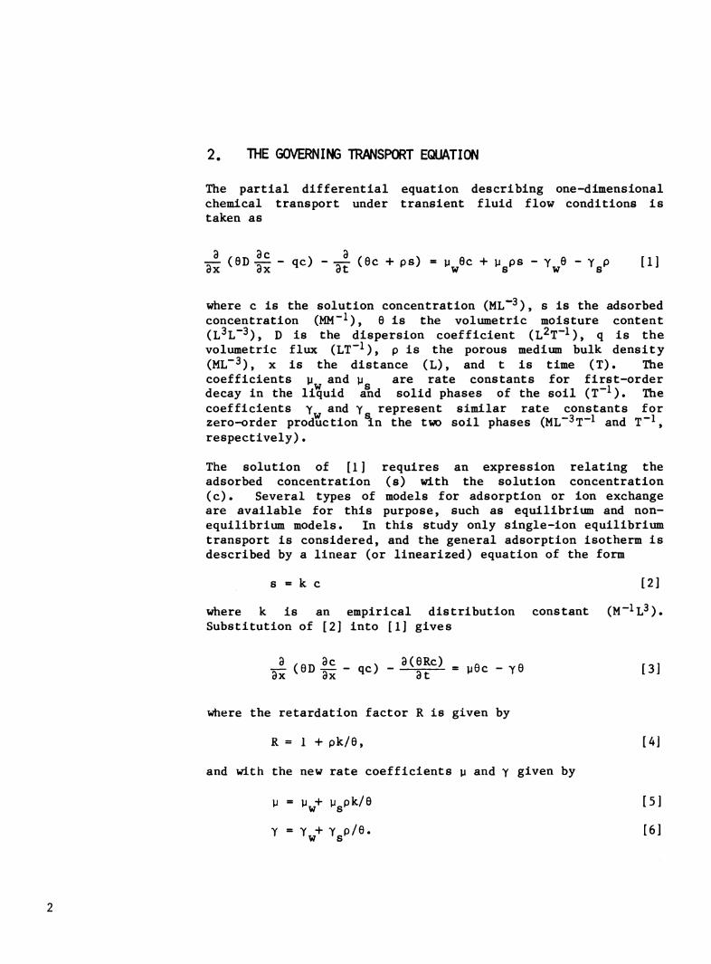
The partial differential equation describing one-dimensional chemical transport under transient fluid flow conditions is taken as
gi (6D 1^ - qc) - ^ Oc + PS) = y^ec + y^ps - Y„6 - Y3P [1]
where c is the solution concentration (ML"^), s is the adsorbed concentration (MM"^), 0 is the volumetric moisture content (L^L*"^), D is the dispersion coefficient (L^T"^), q is the volumetric flux (LT"^), p is the porous medium bulk density (ML"^), X is the distance (L), and t is time (T). The coefficients p and \i are rate constants for first-order decay in the liquid and solid phases of the soil (T~^). The coefficients y and y represent similar rate constants for zero-order production m the two soil phases (ML~^T~^ and T"^, respectively)•
The solution of [1] requires an expression relating the adsorbed concentration (s) with the solution concentration (c). Several types of models for adsorption or ion exchange are available for this purpose, such as equilibrium and non- equilibrium models. In this study only single-ion equilibrium transport is considered, and the general adsorption isotherm is described by a linear (or linearized) equation of the form
s = k c [2]
where k is an empirical distribution constant (M""^L^). Substitution of [2] into [1] gives
i^ere the retardation factor R is given by
R = 1 + pk/e, [4]
and with the new rate coefficients y and y given by
y = y^+ ygPk/6 [5]
Y = Y^+ YgP/e« 16]

When the volumetric moisture content and the volumetric flux remain constant in time and space (steady-state flow), the transport equation reduces to
.2 , , P, 0 c oc ^ OC _ f-j.
ÔX
where v (=q/9) is the interstitial or pore-water velocity. Equation [7], or its appropriate simplifications, has found widespread application in soil science, chemical and environ- mental engineering, and water resources. Some of the known applications include the movement of ammonium or nitrate in soils (Gardner 1965, Reddy et al. 1976, Misra and Mishra 1977),^ pesticide movement (Kay and Elrick 1967, van Genuchten and Wierenga 1974), the transport of radioactive waste materials (Arnett et al. 1976, Duguid and Reeves 1977), the fixation of certain iron and zinc chelates (Lahav and Hochberg 1975), and the precipitation and dissolution of gypsum (Kemper et al. 1975, Glas et al. 1979, Keisling et al. 1978) or other salts (Melamed et al. 1977). Transport equations similar to [7] have also been applied to saltwater intrusion problems in coastal aqui- fers (Shamir and Harleman 1966 ), to thermal and contaminant pollution of rivers and lakes (Cleary 1971, Thomann 1973, Baron and Wajc 1976 , DiToro 1974), and to convective heat transfer problems in general (Lykov and Mikhailov 1961^ Carslaw and Jaeger(;959 )•
3. INITIAL AND BOUNDARY CONDITIONS
This compendium gives analytical solutions of [7] subject to various initial and boundary conditions. The general initial condition is
c(x,0) = f(x) (t = 0) [8]
where f(x) can take on several forms: a constant value with distance, an exponentially increasing or decreasing function with x, or a steady-state type distribution for production or decay. Two different boundary conditions can be applied at x = 0: a first- or concentration-type boundary condition of the form
c(0,t) = g(t) (x = 0) [9a]
or a third- or flux-type boundary condition of the form
^The year in italic, when it follows the author's name, refers to Literature Cited, p. 98.

-D 11+ ve = V g(t) (x = 0) [9b]
where g(t) also can take on several distributions, such as a constant value in time (continuous feed solution), a pulse-type distribution, or an exponentially increasing or decreasing function with time« Note that [9b] does lead to conservation of mass inside a soil column, whereas [9a] may lead to mass balance errors when applied to displacement experiments in which the tracer solution is injected at a prescribed rate. These errors can become significant for relatively large values of the ratio (D/v).
For the lower boundary, the following condition can be applied
1^ («>,t) - 0. [10a]
This condition assumes the presence of a semi-infinite soil column« When analytical solutions based on this boundary condition are used to calculate effluent curves from finite columns, some errors may be introduced* An alternative boundary condition, one that is used frequently for dis- placement studies, is that of a zero concentration gradient at the lower end of the column:
If (L,t) « 0 [10b]
where L is the column length. This condition, which leads to a continuous concentration distribution at x=L, has been discus- sed extensively in the literature (Wehner and Wilhelm 1956, Pearson 1959^ van Genuchten and Wierenga 1974^ Bear 1979). In our opinion, no clear evidence exists that [10b] leads to a better description of the physical processes at and around x=L than [10a]« Moreover, boundary condition [9b] does lead to a discontinuous concentration distribution at the column entrance (x«0) and, as such, seems to contradict the requirement of having to have a continuous distribution at x=L.
In this study, we present analytical solutions for both lower boundary conditions ([10a] and [10b]). Because of the relatively small influence of the imposed mathematical boundary conditions, the analytical solutions for a semi-infinite system should provide close approximations for analytical solutions that are applicable to a physically well-defined finite system, especially for laboratory soil columns that are not too short.

Boundary condition [10a] cannot be applied to Eq. [7] for the particular case when ^i = 0 and y > 0» The lower boundary con- dition for a semi-infinite system that is subject to zero-order production only (no first-order decay) is
ÔC
ax (oo,t) = finite. [10c]
Table 1 summarizes the various mathematical models for which analytical solutions are given in the next section. The gov- erning equations and associated initial and boundary conditions are grouped into three categories: Category A, where the gov- erning transport equation has no production and decay terms (y = ji = 0); category B, for zero-order production only (y ^ 0; [i = 0); and category C, for simultaneous zero-order production and first-order decay (y ^ 0, |i ^ 0). No special category is given for those models in which the transport equa- tion has only a first-order decay term (y = 0; ji ît 0). The analytical solutions for these cases follow immediately from those of category C by simply putting y = 0 in the various expressions. A similar reduction from category C to category B, by assuming ^i = Ü, is mathematically not possible because of divisions by zero.
Table 1.—Summary of mathematical models for which analytical solutions are given
Governing Equation
%t \^2 %x
Initial condition f(x)l
Upper boundary condition
Case Type2 g(t)3 Lower boundary
condition**
Al A2 A3 A4
A5
A6 \C2
Ci —do— —do— —do— (0 < X < X, ) (x > xp —do-
1 C^ (pulse)5 3 —do— 1 —do— 3 —do—
1 —do—
3 —do-
Semi-infinite, —do- Finite. —do—
Semi-infinite.
—do—
See footnotes at end of table.

Table 1.—Summary of mathematical models for which analytical solutions are given—Continued
Governing Equation
at = D ö^*' - V ^^ 0x2 ^ôx
Upper boundary
Initial condition
condition
Lower boundary Case f(x)l Type2 g(t)3 condition**
A7 C, + C, e-^ 1 C (pulse) 5 —do— A8 A9
^ ~do~
Ci
3 ~do~ 1 C + C. e" 3 —do—
-\t ~do~ Semi-infinite.
AlO -do~ —do- All ~do~ 1 ~do~ Finite. Al 2 ~do~ 3 —do— —do—
Governing Equation
-, ÔC T. Ô c ÔC . ôt ^2 ôx ^
ôx
Bl NA^ 1 Co Semi-inifite. B2 —do— 3 —do— —do— B3 —do— 1 —do— Finite. B4 —do~ 3 —do— —do— B5 Ci 1 CQ (pulse) Semi-infinite. B6 —dS— 3 —do— —do— B7 —do— 1 —do— Finite. B8 —do— 3 —do— —do— B9 ST-ST^ 1 —do— Semi-infinite. BIO —do— 3 —do— —do— BU —do— 1 —do— Finite. B12 —do— 3 —do— . . —do— B13 ^i 1 C + C^ e"'''^
a , b —do—
Semi-infinite. B14 —do— 3 —do~ B15 —do— 1 —do— Finite. B16 —do— 3 —do— —do—
See footnotes at end of table.

Table 1.—Summary of mathematical models for which analytical solutions are given—Continued
Governing Equation
^ôt ÔX
ÔC
Upper boundary
Initial Condition
condition
I Lower boundary Case f(x)l Type 2 g(t)3 condition**
Cl NA^ 1 Co Semi-infinite. C2 —do~ 3 -dl- —do— C3 —do— 1 —do— Finite. C4 —do— 3 —do— —do— C5 Ci 1 C- (pulse)5 Semi-infinite. C6 —dS— 3 ° —do— —do— C7 —do~ 1 —do— Finite. C8 —do— 3 —do— —do— C9 ST-ST7 1 —do— Semi-infinite. CIO —do~ 3 —do— —do— Cll ~do~ 1 —do— Finite. C12 C13
—do—
^i
3 1
__do— C + C^ e ^"^
—do—
—do— Semi-infinite.
C14 —do— 3 —do- C15 —do— 1 —do— Finite. C16 ~do~ 3 —do- —do—
^f(x) in equation [8]. 2'!' for a first-type boundary condition (equation [9a]); '3' for a third-type boundary condition (equation [9b]).
3g(t) in Eq. [9a] or [9b]. ^Equation [10a] or [10c] for a semi-infinite system; equation [10b] for a finite system. ^Indicates a pulse-type application:
g(t) 10
(0 < t < t ) o
(t > t^) o
^Not applicable; steady-state solution. ^Steady-state type initial distribution.
4. LIST OF ANALYTICAL SOLUTIONS
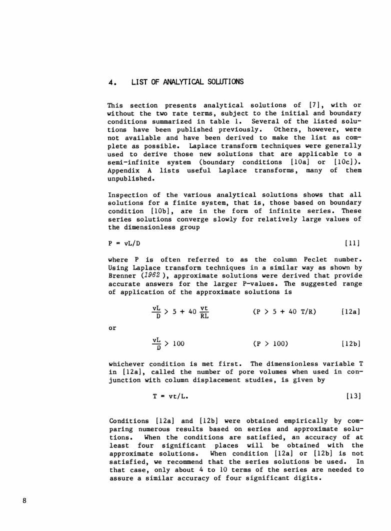
This section presents analytical solutions of [7], with or without the two rate terms, subject to the initial and boundary conditions summarized in table 1. Several of the listed solu- tions have been published previously. Others, however, were not available and have been derived to make the list as com- plete as possible. Laplace transform techniques were generally used to derive those new solutions that are applicable to a semi-infinite system (boundary conditions [10a] or [10c]). Appendix A lists useful Laplace transforms, many of them unpublished.
Inspection of the various analytical solutions shows that all solutions for a finite system, that is, those based on boundary condition [10b], are in the form of infinite series. These series solutions converge slowly for relatively large values of the dimensionless group
vL/D [111
where P is often referred to as the column Peclet number. Using Laplace transform techniques in a similar way as shown by Brenner (2962 ), approximate solutions were derived that provide accurate answers for the larger P-values. The suggested range of application of the approximate solutions is
^>'-'°s or
vL > 100
(P > 5 -f 40 T/R)
(P > 100)
[12a]
[12b]
whichever condition is met first. The dimensionless variable T in [12a], called the number of pore volumes when used in con- junction with column displacement studies, is given by
T = vt/L. [13]
Conditions [12a] and [12b] were obtained empirically by com- paring numerous results based on series and approximate solu- tions. When the conditions are satisfied, an accuracy of at least four significant places will be obtained with the approximate solutions. When condition [12a] or [12b] is not satisfied, we recommend that the series solutions be used. In that case, only about 4 to 10 terms of the series are needed to assure a similar accuracy of four significant digits.
A. Solutions for No Production or Decay
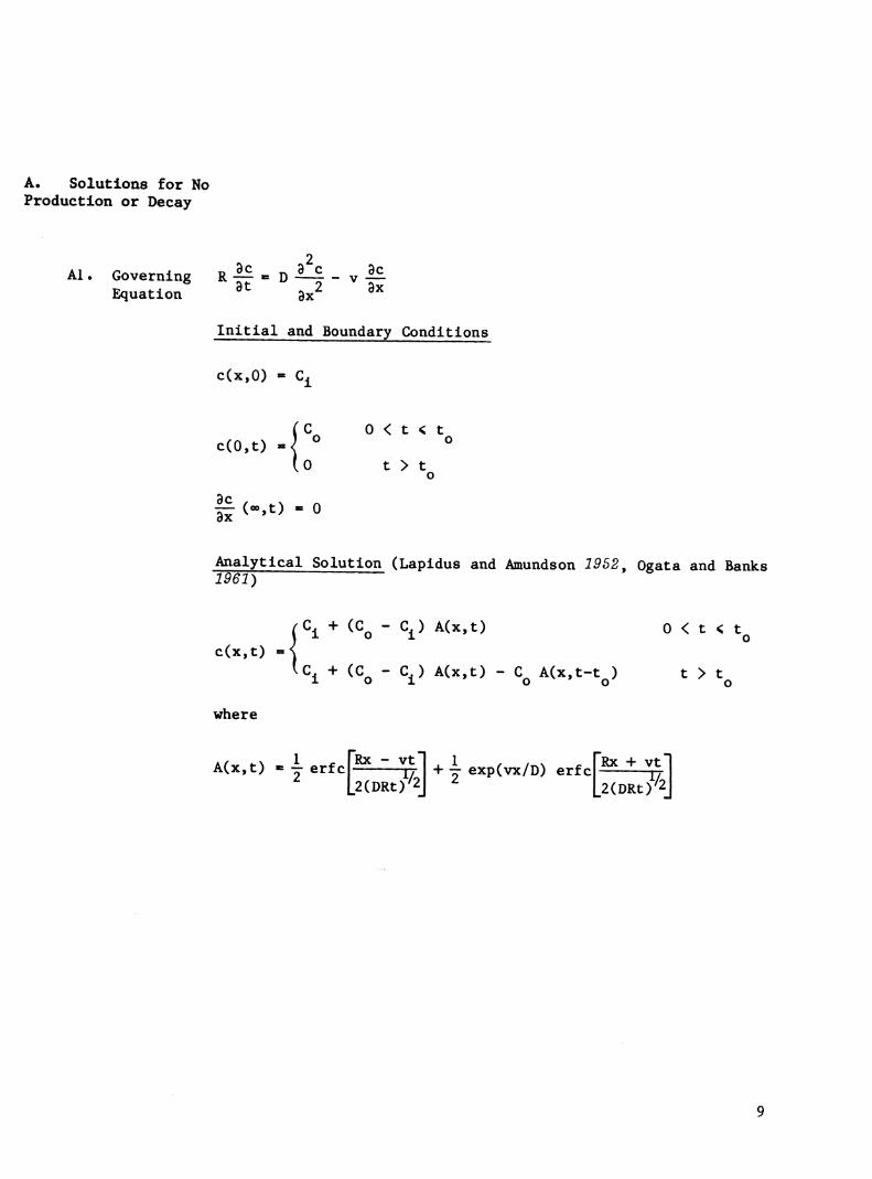
2 Al. Governing R |£ = D -^ - v -^
Equation ^^ 3x^ ^*
Initial and Boundary Conditions
c(x,0) - C^
(C 0 < t < t c(0,t) J °
t > t o
H (..t) - 0
Analytical Solution (Lapidus and Amundson 1952, Ogata and Banks T96J)
(^1 "^ ^^o " ^i^ ^^""'^^ ^ < ^ ^ ^o c(x,t) -<
ic + (C - C ) A(x,t) - C A(x,t-t ) t > t •*- V i o o o
where
A(x,t) --l i erfcpíL^l + 1 exp(vx/D) erfcp^JlJitl 2 L2(DRt)/2j 2 L2(DRt72j

A2. Governing R — = D —r- - v — Equation "^"^ 3x^ "^^
Initial and Boundary Conditions
c(x,0) = C^
(vC 0 < t < t
^"^ x=0 (0 t > t ' ^ o
Analytical Solution (Mason and Weaver 1924, Lindstrom et al. 1967, Gershon and Nir 1969),
Í ^1 "^ ^^o " ^1^ A(x,t) 0 < t < t^ c(x,t) =S
^ ^i "^ ^^o ~ *^i^ ^^"^'^^ " ^o A(x,t-t^) t > t^
where
2 ^/2 2 */ ^x 1 iT fRx - vt"| _^ /V t. f (Rx - vt) , A(x,t) - - erfc ——IT + (^) exp[ ^^g^—]
2 j (1 + ^ + ^) exp(vx/D) erfc
[Rx + vtl
2(DRt)^J
10

2 A3. Governing R|^=D^-VÍ^
Equation ^^ dx^ ^^
Initial and Boundary Conditions
c(x,0) = C^
(C 0 < t < t c(O.t) =] °
(o t > t o
t <■■•'> ■ °
Analytical Solution (Cleary and Adrian 1973 )<
c(x,t)
where
C. + (C - C.) A(x,t) 0 < t < t i o i * o
C^ + (C^ - C^) A(x,t) - C^ A(x,t-t^) ^ > ^o
,2, 3 X 2^ ß Dt o o ^ / ™ \ rVX V t m ,
« 2ß^ 8in(—) expido - 4DR - ;-2-l
A(x.t) " 1 - I ^ ^ 2
K^ ^2D^ ■'ID^
and where the eigenvalues ß are the positive roots of the equation
ßm^°^(^m> -^15=0
11
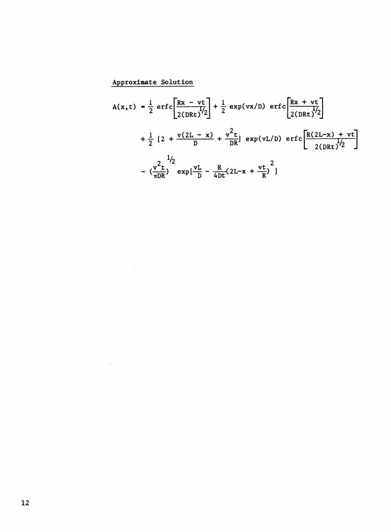
Approximate Solution
A(x,t) »y 1 -: PRX - vt"| ^1 / /TxN * FRX + vt*] T- erfc u + T exp(vx/D) erfc ^ 2 L2(DRt)^2j 2 L2(DRt)/2j
[R(2L-x) + vtl . 2(DRt/''2 J
+ 1- [2 +1(21^^ Aj ^,p(^L/D) erfc
2 '/2 2 ,V tv rVL R /OT _!_ Vtv 1 -^^^ «^Pl-D-4Dt<2L-x+—) ]
12

A4. Governing Equation
ôt g^2 ÔX
Initial and Boundary Conditions
c(x,0) = C,
(-D If + vc) ■1 vC
x=0 fO
0 < t < t
t > t
tí ''■•" - "
Analytical Solution (Brenner 1962, see also Bastian and Lapidus 2956)'
c(x,t) =.
^1 "^ ^^o " ^i^ A(x,t)
^1 "^ ^^o " ^1^ A(x,t) - C^ A(x,t-t^)
0 < t < t
t > t
where
A(x,t)
1 - I- m-1
2vL ß X
vL fix fVX V t "^m ^ 1 exp I-
^ ß. K -°«(-r-> + iïï «^-í-r>J "^ 2D 4DR 2 2
r^2 . /VLv , VLi r^2 , /VLx 1
•2D'
and where the eigenvalues ß are the positive roots of
^m . vL ß cotCß ) - -=- +717 = O ^m ^m vL 4D
13

Approximate Solution (Brenner 1962)
A(x, 2 '/2 ,„ o
L2(DRt)'2J
V2
2 [2I.-X H. 3|i + ^C2L-x +:|)'j exp(,I./D) .rf c fc^isl+vt] L 2(DRt)'2 J
14

2 A5. Governing R||=D^-V||
Equation 8x
Initial and Boundary Conditions
C 0 < X < X
c(x,0) =S vC^ X > X 1
/C 0 < t < t I o o
c(0,t) =< Í0 t > t
o
If (..t) - 0
Analytical Solution
c(x,t) -
(S "^ ^^r S^ A(x,t) + (C^- Cj) B(x,t) 0 < t < t^
^C- + (C- C„) A(x,t) + (C - C, ) B(x,t) - C B(x,t-t^) t > t^ ¿ 1 ¿ 01 o o o
where
I R(x+x, ) + vt" [RÍX-X ) - vt"! PRíX+X ) + V A(x,t) - \ erfc ^—j] + ^ exp(vx/D) erfc rj-
2 L 2(DRtf2 J 2 1^ 2(DRtf2
B(x.t) = I erfcF^L^I + j exp(vx/D) erfcp^L±^l 2 L2(DRtf2j 2 [2(DRt)/2j
15

A6. Governing Equation
^ 8c ^ 3c 3c 3t ^2 3x 3x
Initial and Boundary Conditions
c(x,0) =
C 0 < X < X
X > X,
(-D||+VC)
vC
x=0 VO
0 < t < t
t > t.
II (.,t) . 0
Analytical Solution [see also Jost (1952, p. 50) and Lindstrom and Boersma (1971)]
c(x,t) =
C^ + (C^- C2) A(x,t) + (C^- C^) B(x,t) 0 < t < t.
S "^ ^^r ^2^ A(x,t) + (C^- C^) B(x,t) - C^ B(x,t-t^) t > t^
where
A(x,t) ■j erf c R(x-x )-vt
2(DRtr2 nDR ^ D R / -._ ^ vt. 1 ^x+x^ + —) ]
1 v(x+x ) 2 " i ^^ "*" D "^ ~DR^ exp(vx/D) erfc
R(x+x.) + vt
VÖ' 2(DRt)'2
B(x,t) » 4 1 , [BX - vtl ^ .V t 2 ^/2 2
) exp[ /.TM>. 1 4DRt
- y (1 + ^ + ^) exp(vx/D) erfc [Rx + vtl 2(DRty2j
16

A7. Governing R — = D —- " ^ TZ Equation ^ ôx"^ ^^
Initial and Boundary Conditions
c(x,0) »= Cj^ + C2 e"^^
ÍC 0 < t < t o o
O t > t o
I; (-'> " " Analytical Solution
c(x,t) =
i^l ■*■ ^^o " ^1^ A(x»t) + C2 B(x,t) 0 < t < t^
Cj + (C^ - C^) A(x,t) + C2 B(x,t) -C^ A(x,t-t^) t > t^
where
A(x,t) =4 1 ^ FRX - Vtl ,1 / /r>\ c TRX + Vtl 2 erfc n- + j exp(vx/D) erfc n.
ÍRX - (v+2aD)t"|
L 2(DRt)''2 J
ERx + (v+2aD)t1 ) 2(DRtr2 J )
B(x,t) = \ exp(¿|^ +^- aK)}2- erfc
vx - exp(— + 2ax) erfc
17

2 A8. Governing l^lj^D-M-vl^
Equation '^^ Ôx^ ^"^
Initial and Boundary Conditions
c(x,0) = C^ + C^ e""''
!vC 0 < t < t o o
O t > t ■ o
ë (..t) - 0
Analytical Solution
c(x,t) =
( ^1 "^ ^^o " ^1^ A(x,t) + C2 B(x,t) 0 < t < t^j
^1 ■*■ ^^o " ^1^ A(x,t) + C2 B(x,t) - C^ A(x,t-t^) t > t^
where
2 ^à 2 */ N A x: I ^^ " VL I . ,V tv r (RX --Vt) ,
A(x.t) = 2 "^HriTT/J ■" ^"^^ ^""P^ 4DRÍE ^ 1 ^ FRX - vt "I . .v__t.
L2(DRt)'2j
2 - j (1 + ^ + ^) exp(vx/D) erfc
B(x.t) = exp(% + ^-ax)|l -
+ 4(1+^) exp(^ + 2ax) erfc 2 aD D
1 ^^.j^fRx - (v+2aD)t1 ^ [ 2(DRt/^2 J
[RX + (v+2aD)t1 ) L 2(DRt)''2 J)
y-Q exp(vx/D) erfc |_2(DRt)'2J
18

A9. Governing R|r*D-^-v|^ Equation °^ bx '^^
Initial and Boundary Conditions
c(x,0) = C^
c(0,t) = C + C, e"^*^ ' a b
H <".^)- » Analytical Solution [see Marino (1974a) for two special cases]
c(x,t) "= C^ + (C^ - C^) A(x,t) -H C^ B(x,t)
where
A(x,t) = -^ erfc \T + TT exp(vx/D) erfc \r 2 L2(DRt)^2j 2 [2(DRt)/2j
B(x,t) - e"^*^
+ jexpl-ii^l erfc L2(DRt)'2j j
and
,, 4XDR/2 y - V (1 2"^
V
19

Alü, Governing Equation ôt g^2 ôx
Initial and Boundary Conditions
x=0 = v(C + a e ^^)
a b
c(x,0) = C,
(-D II + vc)
II (<»,t) = 0
Analytical Solution
c(x,t) = C, + (C - C, ) A(x,t) + C, B(x,t) 1 a 1 D
where
2 V2 A(x.t) = 4 erfcF^^^I + (^
2 L2(DRt)^2j ^R . f (Rx - vt) 1
4DRt
Y (1 + ^ ■»- ^) exp(vx/D) erfc
./' ...\ ~^t 1 V r(v-y)xi ^ I Rx - yt Kx,t) = e {TTZZTT expL^ ,^^ ] erfcl i-
2XDR
L2(DRt)'2j
L2(DRt)^2j exp(vx/D) erfc
and
y = V (1 - —J-) V
V2
20

2 Al 1. Governing R —7 = D 7: "" v —-
Equation 9x
Initial and Boundary Conditions
c(x,0) = C^
c(0,t) = C + C. e"'^*^ a D
If <--^> ■ ° Analytical Solution
c(x,t) = C, + (C - C.) A(x,t) + C. B(x,t) 1 cL 1 D
where
2^ ß^Dt A(x.t) = 1 - I E(ß^,x) exp[2ö " -¡^ - -j-\
m=l L R
B(x,t) = e""^^ [B^(x,t) - B2(x,t)]
2 _,. . XL R ,vxv
B (x,t) = 1 + }, 2 2~ in=l f 2 ,vL _ \L R,
o t 2 2^ ß^Dt ^y« s r«2 , /VLv 1 rvx , ,^ V t m i - E(ß^.x) [ß^ + (^) ] exp[^ + xt - ^^ - —2-]
B2(x,t) - 5; 2 2 m=l r 2 ,vLv _ XL R,
^Pm ^ 4D^ D ^
and
ß x
E(ß„,x) 2ß^ 8in(-f-) m L
r/^2 . ,vL. . vL,
21
The eigenvalues ß^ are the positive roots of
ß cot(ß ) + ^ = O m m ¿u
The term Bj^Cx) converges much slower than the other terms in the series solution. This term, however, can be expressed in an alternative form that is much easier to evaluate:
, , , ^^P^ 2D ^ V-+v^ ^^^ 2D ^ B (x) = ^ U + C-^) exp(-yL/D)]
where
y = V (1 ^) V
Approximate Solution
A(x.t) = j erfcf^ ' ^^^l + j exp(vx/D) erfcl"^ "^ ^¿1 [2(DRt)'2J ^ L2(DRt)'2j
. 1 ,, . v(2L-x) . v^t, / T /T^^ Í rR(2L-x) + vt1
2 '''2 2 ,V tv rVL R /OT -l_ Vt. 1 - ^^ «^Pt^- 4DF^2L-X+-^) ]
BCx.t) = e"''^ B3(x,t)/B^(x)
where
22

c^ .,p,(:aO|^Jzt, «.cp^irïL^]
■" 2^ ^^P^^ -^ ^^^ ^'^^^l-
B^(x) = 1 + (^) exp(-yL/D)
and
V
rR(2L-x) + vt"| L 2(DRt)/2 J
23

A12. Governing Equation
2 ^ de - 3 c 9c
3x
Initial and Boundary Conditions
c(x,0) = C,
(-D If + vc) x=0
a b
3c dx
(L.t) = 0
Analytical Solution
c(x,t) - C^ + (Cg - C^) A(x,t) + C^ B(x,t)
where
A(x.t) «1 - Î E(ß^.x) exp[^-|5|
B(x,t) - e"^*" [Bj(x) - B^Cx.t)]
Bj(x) 1+ I m-1
2 „/- . XL R ,vx.
^^m ^ 4D^ D ^
E(e,'^> Iß^-^^f) 3 exp(g+Xt vit 4DR
B2(x,t)
and
2
L2R
m-1 rß2 + (VL)^ XI¿R,
E(B ,x) m
2vL ^ r^ . m V ^ vL . / m M
-p- ßm ^ßm ^°"^—^ -^ 2D ^^"(—>J 2 2
rn2 ^ /VLv , vL, r^2 ^/VLv 1
24

The eigenvalues ß are the positive roots of
"^m . vL ßr.^Ot(ß) -_-+_= 0
The term Bj^(x) converges much slower than the other terms in the series solution. This term, however, can be expressed in an alternative form that is much easier to evaluate:
B,(x) exp ̂ 2D ^ V-tv^ ^""P^ 2D ^
y+v _ (y-v)
where
y = V (1 j) V
Approximate Solution
r n 2 '/2 2 A/ ^N 1 ^ ^ - vt . .V t. r (Rx - Vt) 1 A(K,t) . j erfcj——ç^ + C^) expl- 4PR, 1
-5'^^-*TI*45«^-*^>'I-
B(x,t) = e ^^ B3(x,t)/B^(x)
where
. j ,r.\ f rR(2L-x) + vtl p(vL/D) erfc JT— L 2(DRt)'2 J
B3(x,t) = (^) exp[-^^^l erfc L2(DRt)'2j
25
L2(DRt)'^2J
- 2Î55 "P<^ * "> "i=P^^-^l L2(DEt)'2j
L 2(DRt)^2 J
(y+v) '° L 2(DRt//2 J
- ^^ exp[-to02,±iZkj erfcp(2L-x) H- ytl L 2(DRt)/2 J
(y.v)2 -- 2D
B^(x) = 1 --telL. exp(-yL/D) (y+v)^
26

B. Solutions for Zero- order Production Only
Bl. Governing ^2^ ^^ Equation D —j " ^ d^ "*" >" ^ ^
(Steady-state) dx
Boundary Conditions
c(0) = C^
4^ (») = finite dx
Analytical Solution
c(x) = c + ^ o V
27
B2. Governing 2 Equation D -^-1 - v ~^ + y = 0
(Steady-state) dx
Boundary Conditions
(-D 4^ + vc) I = vC ^ dx In O x=0
^ (oo) = finite dx
Analytical Solution
c(x) = C + ^^^^ O 2
V
28

B3. Governing ^2^ ^^ Equation D —j - v — + y = 0
(Steady-state) dx
Boundary Conditions
c(0) = C o
i| (L) . 0
Analytical Solution
ß X ^2 m X vL /Vx>
■J lavni
c(x) - c^ + Î 5 5"
where the eigenvalues ß^j^ are the positive roots of
The series solution converges too slowly to be of much use numerically. An alternative and more attractive solution is given by
c(x) - C^ + IJ + If |exp(- :^) - exp[-^]}
29

, . de de „ 34. Governing D —«- - v -^ 1- y = 0
Equation dx (Steady-state)
Boundary Conditions
(-D 4^ + vc) = vC ^^ x=0
ff^^>=° Analytical Solution
c « (-D-) (V ^mt^m ^°«(-r^ + 2D ^^"^—-^^ ^^^^20^
™=1 r«2 ^ .vL. ^ vL, f„2 . ,vL. , I^m-^ ^2D^ ■'"DI f^m-' ^2D^ ^
Where the eigenvalues ß^^ are the positive roots of
The series solution converges too slowly to be of much use numerically. An alternative and more attractive solution is given by
Y^ -^ Y^ il ^..«r^(^~L) -^^^ = ^o "^ V "^ 2 i^ ~ ^""P' D~^^
30

B5. Governing R |£ = D ^ - v || + y Equation ox
Initial and Boundary Conditions
c(x,ü) = C^
1 ° 0 < t < t o
c(0,t) = < (o ^>^o
Il (œ,t) = finite
Analytical Solution (Carslaw and Jaeger 1959, p. 388)
c(x,t)
where
C^ + (C^ - C^) A(x,t) + B(x,t) 0 < t < t^
C. + (C - CJ A(x,t) + B(x,t) - C A(x,t-t ) t > t 1 o i o o o
A(x,t) = -77 erfc ^j + -TT exp(vx/D) erfc \T 2 L2(DRt)/2j 2 L2(DRt)/2j
T>/ ^A Y L ^ (Rx-vt) ^ FRX - vtl
(Rx + vt) , ,^. - - exp(vx/D) erfc 2v
[Rx + vt"| ) 2(DRt//2j ¡
31

B6. Governing R|f"D-^-v||+Y Equation ox
Initial and Boundary Conditions
c(x,0) = C^
/vC 0 < t < t
(-D 1^ + vc) x=0 10 t > t o
ÔX
1^ (»,t) - finite
Analytical Solution (van Genuchten 1981)
c(x,t)
C^ + (C^ - C^) A(x,t) + B(x,t) 0 < t < t
C^ + (C^ - C^) A(x,t) + B(x,t) - C^ A(x,t-t^) t > t^
where
2 ^'^ 2 A/ ^\ 1 £ FRX ~ vtl . fV t. r (Rx - vt) 1 A(x.t) = 2 "'"[j—^2j ■" ^^^ '"P^" ADRt ^
ERx + vt"! 2(DRt)^2j
B(x,t) -^Jt +^(Rx - vt
- y (1 + ^ + ^) exp(vx/D) erfcl
, DR. _ PRX - vt"|
^ [t DR , (Rx + vt) , . ,_. ^ FRX + vt" + 1-5- 5- + TTTjj ] exp(vx/D) erfc jy 2 2v^ ^^'^ L2(DRt)/2
32

2 B7. Governing R |^ = D -2-1 - ^, 21 + y
Equation °^ ox °^
Initial and Boundary Conditions
c(x,0) = C^
ÍC 0 < t < t o o
O t > t o
Analytical Solution
i*^i ■•" ^^o " ^i^ A(x,t) + B(x,t) 0 < t < t^
c(x,t) =<
i "*" ^^o " ^i^ A(x,t) + B(x,t) - C A(x,t-t ) t > t
where
2 ß^Dt A(x.t) = l- I E(ß^.x)exp[|§-|5|--^]
m=l L R
B(x,t) = B^(x) - B^Cx.t)
,, , -, E(ß,,x) 4- exp(i|) B^(x) = l ^
,2 2^ ß^Dt p/o \ YL rvx V t m ,
B^ix.t) = l ^
and
33
L R

E(ß^,x) =
6 X 2ß^ sin(-^)
lß^'îF^'-il
The eigenvalues ß^ are the positive roots of
ßm<=°^^ßm) ■'lïï" °
The term B^Cx) in this solution converges much slower than the other terms. This term, however, can be expressed in an alternative form that is much easier to evaluate (see case B3):
V
Approximate Solution:
A(x,t) - i- erfcf^^^^l + i exp(vx/D) erfcC^ÍL^] 2 L2(DRt)/2j 2 L2(DRt)^2j
. 1 f„ . v(2L-x) . v^t, / T /m £ rR(2L-x) + vtl + 2 12 + -^— + -3R] exp(vL/D) erfc[——i^J
2 '/2 2 /Vtx rVL R /OT _i_ Vtv 1
B(x.t) = X K + I^IÎ^ erf c [Rx - vtl 2(DRO^J
x+vt) , ,^. - FRX + vt"| ■r- exp(vx/D) erfc jj ^"^ L2(DRt)/2j
(Rx+vt)
•^ (4^)^' i^(2^-> -^ vt -K if ] exp(^ - J^(2L-^ -H ^)]
34

, . vR(2L-x)-DR ^ R ,-,T j. vts , ,vL. [t + 2 "'' 40 (2L-X + —) ] exp(—) erfc
2v
DR rv(x-L), - —=■ exp[—^^tr—-] erfc 2v
[R(2L-x) + vt] 2(DRt/'^2 J
tR(2L-x) - vt] (
2(DRtr2J /
35

B8. Governing R||"D-^-V||+Y Equations ox
Initial and Boundary Conditions
c(x,0) = C^
ft 0 < t < t o c
.„ „ 0 t > t
Analytical Solution
/C^ + (C - CJ A(x,t) + B(x,t) 0 < t < t 1 i o i o c(x,t)
where
^i ■*■ ^^o " ^i^ A(x,t) + B(x,t) - C^ A(x,t-t^) t > t^
2^ ß^Dt ./• \ , VT,/« \ fVX vt nil A(x.t) = 1-1 E(ß^,x) exp[-^ - j^ - -J-]
m"l L R
B(x,t) = Bj(x) - B2(x,t)
,, , % E(ß,>x) 4- expCg) B^(x) = I 2
T2 2^ ß^Dt 17/-n \ YL fVX V t m 1
» '^ißm^'^^D^^PflD-ÄDR-727-1 B^Cx) = I -2 ^-^
36

and
2vL - r^ ,'^m..vL . , ^m^v,
E(ß^,x) . ^_JL-^ÎL___L 2D L_
tßm-' ^2D> -"ill tßm-' W ^
The eigenvalues ß^^ are the positive roots of
The term Bj(x), which also appears in the steady-state solution (case B4), converges much slower than the other terms in the series solution. This term, however, can be expressed in an alternative form that is much easier to evaluate:
V
Approximate Solution
Rx - vt)^, 4DRt ^
1 2 j (1 + -^ + ^) exp(vx/D) erfc
L2(DRt)^2j
2 '/2 2 -L (^^ ^\ n j. v.^- . vtvi rVL R .^_ . vtv 1 ■" ^^SR-> ^^ ^ ÂD^2L-x + —)] expl— - ■45^(2L-x + —) ]
- - [2L-X + -^ + -^(ZL-x + —) ] exp(vL/D) erfc rR(2L-x) + vtl
L 2(DRt)^2 J
37

( t_/2 . ^ . 2DR, r (Rx - vt)^, (X;;ñR> (Rx + Vt + -—) exp[- y,nD. ] ^4TIDR' ^^^ • ^" " ^r^ ^^^I'l ÄDRT
+ í<= DR ^ (Rx + vt)^, , ,,^, + I7 - —9 + TT;^ ] exp(vx/D) erf c 2 ., 2 4DR 2v
DR fV(x-L), - —2 gxpt D ^ ^^^*^
2v
[Rx + vt"! 2(DRtr2j
rR(2L-x) - vt"| L 2(DRtr2 J
2
+ 2 H - —2ñ ^ —Ö ^^^-^ + -g-)(2L-x + -—) 2v ''^ 2D ^ ^
3 3 + -^(2L-x + ^) ] exp(vL/D) erfcl
ÖD-" *" L 2(DRt)*'
rR(2L-x) + vtl L 2(DRt)^2 J
6D
^HB} ^^P t-D - 4DF^2L^ + l-¡
38
B9. Governing R |£ . D ^ - v || + y Equation ox
Initial and Boundary Conditions
c(x,0) = C^ +^
ÍC 0 < t < t o o
O t > t o
Il (œ,t) = finite
Analytical Solution (Carslaw and Jaeger 1959^ p. 388)
C^ + -^ + (C - C^ ) A(x,t) 0 < t < t i V o i * <
C^ -H^ + (C - CJ A(x,t) - C A(x,t-t ) t > t i VO j^^N»^ o'o o
where
A(x,t) = 1 - TRX - Vtl _^ 1 / /T^^ r r^X + Vtl
= 2 ^^^^ lA r 2 ^xp(vx/D) erfc jr ^ L2(DRt)^2j ^ L2(DRt)^2j
Comment ; Note that the initial condition is of the same form as the steady-state solution for the same boundary conditions (case Bl).
39

2
BIO. Governing R-|r=D^-v|j+Y Equation ôx
Initial and Boundary Conditions
e(x.O) = c. -fXÇZÎÎËl V
!vC 0 < t < t o o
.... o t > t • O
1^ («,t) = finite
Analytical Solution
+ X(v^+(c-n ) A(x.t) _ i ¿ 0 1
c(x,t)
+ y(vyH-D) ^ ^ç _ ^ . A(x,t) - C A(x,t-t ) t > t i 2 o i ' 0 0 c
O < t < t o
where
2 ^^2 2 Kl ^\ 1 Í fRx - vt"! . /V t. f (Rx - vt) ,
2 j (1 + ^ + ^) exp(vx/D) erfc
L2(DRt)^2j
Comment: Note that the initial condition is of the same form as the steady-state solution for the same boundary conditions (case B2).
40

2 Uli. Governing R|r=D-^-v|^+Y
Equation ôx
Initial Condition
c(x,0) = A(x)
Note that the initial condition is of the same form as the steady-state solution for the same boundary conditions (case B3).
Boundary Conditions
!C 0 < t < t o o
O t > t o
i <^.^> - ° Analytical Solution
/ A(x) + (C^ - C^) B(x,t) 0 < t < t^
c(x t) = I ' A(x) + (C - C.) B(x,t) - C B(x,t-t^) t > t^
where A(x) is exactly the same as the initial condition, and where
ß X 2^ ß^Dt o ^ j / lû \ fVX V t m ,
» 2 ß^ 8in(^ exp[^ - -j^ - -^]
B(x,t) =1-1 ^ ^ 2
The eigenvalues ßjj^ are the positive roots of the equation
41

Approximate Solution
A(x,t) = 4 = I erfcfe-llj;!] + 1 exp(vx/D) erfcr-^L±j;^l L2(DRt)/2j 2 L2(DRt)/2j
+ 1 [2 + v(2L:20 + Aj exp(vL/D) erfcF^^^^-^) ^,/^] L 2(DRt)'2 J
V2
42

.12. Governing R |£ = D ^ - v || + y Equation ox
Initial Condition
c(x,0) = A(x)
Note that the initial condition is of the same form as the steady-state solution for the same boundary conditions (case B4).
Boundary Conditions
ÍC Ü < t < t o o
.. . ü t > t O
i <^-'> - ° Analytical Solution
c(x,t)
A(x) + (C - C.) B(x,t) 0 < t < t
A(x) + (C - C.) B(x,t) - C B(x,t-t ) t > t o 1 o o o
where A(x) is exactly the same as the initial condition, and where
B(x,t) =
o T ß X . ß X 2^ ß^Dt 2vL ^ r« / ni V . vL _, ,^m V 1 rvx v t m ,
» — ^ % "^^—> ■" 2D «i-(—>J --PÍ2D - 45^ - 72:^ 1 - I "-^ 2 2
^~1 r^2 ^ ^vLv ^ vL, r^2 . /VLx 1
The eigenvalues ß^^ are the positive roots of
43
^m ^m vL 4D
Approximate Solution
B(x,t) =i 2^2 ,„ ^0
1 ^^^^ffoc - vtl . /V tv r (Rx - vt) ,
[Rx + Vtl 2(DRt)^2j
1 vx v-^t 2 (1 + "^ ■*" -^^ exp(vx/D) erfc
2 '/2 2 •^ ^IDT^ 11 -^ 4D^2L-x + —)] exp[— - ;^(2L-x + —) ]
V roT „ j. 3vt . v,-^ , vtv , / T /TNN ^ rR(2L-x) + vtl --¡r [2L-X +-^^ +-T;^2L-X +-5-) ] exp(vL/D) erfc -i^ '—n— ° 2R 4D R L 2(DRt)/2 J
44
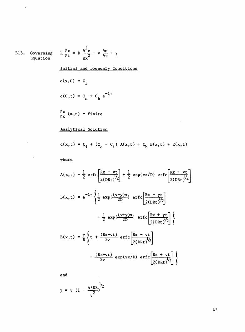
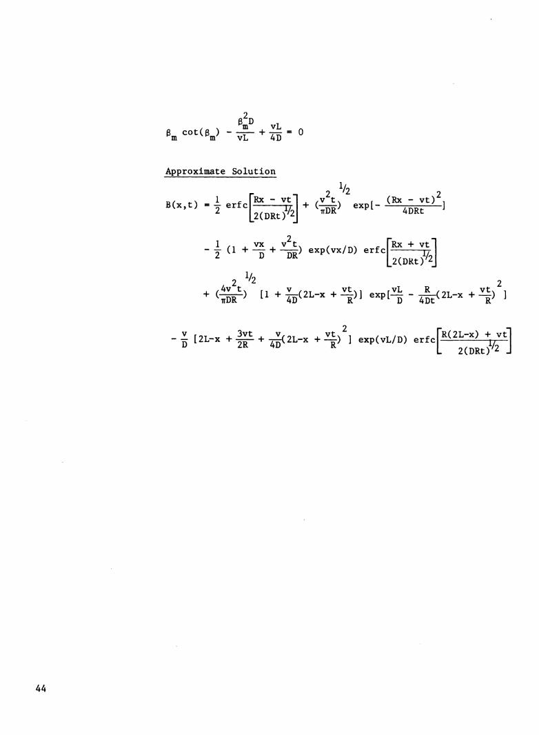
2 B13. Governing R |^ = D -^ - v |^ + y
Equation ox
Initial and Boundary Conditions
c(x,0) = C^
c(0,t) = C^ + C^ e"'''^
II (»,t) = finite
Analytical Solution
c(x,t) = C^ + (C^ - C^) A(x,t) + C^ B(x,t) + E(x,t)
where
A(x,t) - ^
B(x.t) =e-^^Uexp[l:iJg^] erfc L2(DRt)^2j
r?r -^ Y (^ -L (Rx-vt) - FRX - vtl E(x,t) = "¿- < t + -^—r erfc TT ^ ( 2^ L2(DRt)/2j
(Rx+vt) . /^.x ^ FRX + vt - -^—TT ^ exp(vx/D) erfc rr ^^ L2(DRt)^2
and
y = V (1 2~)
45

2 B14. Governing R |r = D -^ - v |^ + v
r. . ôt ,2 ÔX ' Equation 9x
Initial and Boundary Conditions
c(x,Ü) = C^
(_D|£+VC)| = V(C + C, e"'^'') ÔX \Q ab
Il («,t) = finite
Analytical Solution
c(x,t) = C. + (C - C,) A(x,t) + C, B(x,t) + E(x,t) 1 a 1 D
where
2 ^^2 2 A(x t) = ^ erfcf^ " ^i*^! + i^^-^) exp[- ^^ " ^<^> 1 AU.t; 2 [2(DRt)/2j ^R ^DRt J
[Rx_+_vt"l
2(DRt/^^
2 " i ^^ "*■ "^ "^ "^^ exp(vx/D) erfc
2 2j-j^ exp(vx/D) erfc
L2(DRt)'2j
46

E(x,t) X L j. 1/1, * ^ DR. - I Rx - vt n \t + vHRx - vt + —) erfc 2v' L2(DRt)'2j
-0"<^-'-^>-P'-^Í^TÍi#l
. rt PR . (Rx + vt) 1 , ,^. ^ ÍRx+vt" + [2 2 "^ 4DR ^ exp(vx/D) erfc rr
"^ 2v^ ^'^'^ L2(DRt)'2
and
y = V (1 r-) V2
47

2
B15. Governing R|f=I^-^-'^|f+Y Equation dx
Initial and Boundary Conditions
c(x,0) = C^
c(0,t) = C^ + C^ e"^^
Analytical Solution
c(x,t) = C, + (C^ - C,) A(x,t) + C. B(x,t) + F(x,t) 1 a 1 D
where
2^ ß Dt rVx V t m A(x.t) = 1-1 E(ß^.x) exp[^ - ioè - -Vl m=l L R
B(x,t) = e"-^*" [B^(x) - B^Cx.t)]
2 „,„ ^ AL R ,vxv
«0 E(ß_,,x) =r- exp(-;r-) B l(x) = 1 + I —^ D -'»-^20'
o , 2 2^ ß^Dt ^/^ \ r^2 , /VL\ 1 ivx , ,^ V t m 1
- E(ß^.x) [ß^ + (^) ] expl2Ö+ At -^- -2-1
m=l ,1 ^ ,vL.^ AL^R,
F(x,t) = F^(x) - F^Cx.t)
48

o. E(ß x) J¿- exp(^) FjCx) = I —^ 2 _2D_
-2 2^ ß^Dt !?/■ o N yL rVx V t mi
« ^(Pm'^) D «^PÍ2D-4DR-X"^ F2(x,t) - I 2 ^^^-
and
ß X 2ß^ sin(-5^)
E(ßm'^> ^^ r— ^ O T -^ T rr»2 . /VLv , vLi
The eigenvalues ß^j^ are the positive roots of
The terms Bj^(x) and Fj^Cx) converge much slower than the other terms in the series solution. Both terms, however, can be expressed in alternative forms that are much easier to evaluate:
„ , , ^^P^ 2D ^ Srfv^ ^^P^ 2D ^ B (x) » ^ U + (^) exp(-yL/D)l
where
V2
V '
and
y « V (1 - —^)
FjW.J:ï + i||exp(-ii)-.xp[:^il
49

Approximate Solution
A(x,t) = ^ 1 ^ [RX - vt"| ^1 / ,^. ^ FRX + vt"| = -r erfc u + T exp(vx/D) erfc rj
2 L2(DRt)/2j 2 L2(DRt)/2j
rR(2L-x) + vt"| L 2(DRt)^2 J 2 ^ ^^ ■ 2(DRt)
2 '/2 2 ,V tv rVL R ,^_ . Vtx 1
B(x,t) = e"''^ B3(x,t)/B^(x)
(y-v) _,<itZ)ílM¡i 1.1-r, r^<^'--''> - yfl 2(y^) "Pi 2D 1 "n 2(„R,)V2j
I (y>v) ,(v-y)»<-2yL, rR(2L-K) l- ytl 2(y-v) -"> 2D 1 "'1 2(DRt//2j
rR(2L-x) + vt"| L 2(DRt)''2 J
^2 ^^
^^"^ ° ' 2(DRt)
B^(x) = 1 + (^) exp(-yL/D)
and
^ ( 2v L2(DRt//2j
(Rxt-vt) , ,^. ^ = exp(vx/D) erfc [Rx + vt"| 2(DRt?^2j
50

- ^4^>'' í^<2^-> -^^-^^ -Pí^ - 4IF<2^- -^>'I
^^ ,.K(2^.^(..-. .Z|)^ expCl) erfc[M2^^]
2v
[R(2L-x) - vtl I . 2(DRt//2 J)
51

B16. Governing R |^ - D-^ - v |^ + Y Equation dx
Initial and Boundary Conditions
c(x,0) = C,
(-D If * vc) x«0
v(C + a e"^^) a b
H <'••'> ■ »
Analytical Solution
c(x,t) = C^ + (C^ - C^) A(x,t) + C^ B(x,t) + F(x,t)
where
A(x,t) = 1 - I E(a^,x) exp[ m=l
vx 2D
2^ e^Dt V t m 4DR L2R
B(x.t) - e"^^ [Bj(x) - B2(x,t)]
Bj(x) ^ 2 2
^(^m'^) i^^-^^i) 1 exp[||+Xt 4DR B^Cx.t)
L^R
m=l rg2 + (VL ^ XÍ¿Ri ^^m ^ 4D'' D ^
F(x,t) = F^(x) - F^Cx.t)
52

F,(x,t) = I
.2 2^ B Dt r./-/, \ r'^ rVx V t m 1
2 m=l r^2 , .vL. 1
and
E(ß .X) - "^ "^ "^ ^ 2D L
2vL . r- .'^^m V , vL . / m
The eigenvalues ß^ are the positive roots of
The terms B^Cx) and Fj(x) converge much slower than the other terms in the series solution. Both BjCx) and F^Cx), however, can be expressed in alternative forms that are much easier to evaluate:
B (x) = '^
i^-i^»p<-^^'«'
where
/I 4\DR/2 y = V (1 ^)
V
and
53
Approximate Solution
lu .2
*<-'-^4¡3]^<^ V2
V r (RX - Vt) 1
1 2 - j (1 + ^ + ^) exp(vx/D) erf c
V2
L2(DRt)^2j
2 ^ 2 + ^-^-^ f^ + 4D^2L-x +—)] exp[— - ^(2L-x + —) J
2 - I [2L-X + ^ + 4^2L-x + ^) ] exp(vL/D) erf c
B(x,t) = e"^^ B3(x,t)/B^(x)
ER(2L-x) + vt"!
2(DRt)''2 J
2
2XDR ^""P^"^ "^ '^^^ ^'^^^
2 /OT N 2^ 2
[Rx + vt"| 2(DRt/^2j
v ,v(2L-x) . V t . „ V 1 /-vL . . ^. . rR(2L-x) + vt1 ñDR I—D— + -DR •*■ 3 - XDRJ ^^P^-D "^ '^'^^ ^ [ 2(DRt//2 J
3 V2 2 -^XM<^> -Pt^^^t-^(2L-,-Hl|)]
H.v(z=vl^^pt(vfy)x-2yLj 3,^ J R(2L-x) - ytl (y4v)2 2D |_ 2(DRt)/2 J
- v(ztvi exp[lrz2£t2zli] erfcp^^^LÄJhy^l (y-v)2 2D L 2(DRt)/2 J
54

B (x) = 1 - ^y~''\ exp(-yL/D)
and
F(x,t) = ^ < t + yi(Rx - vt + —) erfc ix i ZV V
Rx - vt
2(DRt)^2 .] 2DRs
- (x;;?^) (Rx + vt +-^) expi- (Rx - vt)'
4DRt
o
j. r*^ DR . (Rx + vt) 1 . ,_. . FRX + vtl
["R(2L-X) - vt"! DR rv(x-L)i ^ -j exp[—^¡r—'-] erfc
2v^ " L 2(DRt)
DR r v(2L-x) . V , vt...^ , 3vt. + —2 ^^ 2D ■*" —9<2L-x + —)(2L-x + —-)
2v^ ^" 2D'^ ^ ^
vt, rR(2L-x) ^ vtl L 2(DRt)^2 J
+ ^(2L-rx +-^) ] exp(vL/D) erfc óD-' *^ L 2(DRt)'
oD
^^^ ^^PI-D-4DF^2L-X+—) ]^
55

C. Solutions for Simultaneous Zero- order Production and First-order Decay
d c do Cl • Governing D —^ " ^ "A jiC + y^O
Equation dx (Steady-state)
Boundary Conditions
c(0) = C o
^ (.) - 0
Analytical Solution
,(,) . X . (C^ - Jt, ...li^i
where
u = V (1 + -^)
56
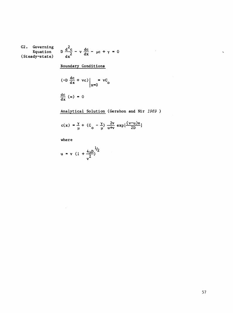
C2. Governing ^2^ ^^ Equation D —j "^"d |ic + y«0
(Steady-state) dx
Boundary Conditions
(-D |£ + vc)
ᣠ(., . 0
« vC x«0 ^
Analytical Solution (Gershon and Nir 1969 )
/ \ Y ^ /n Y\ 2v r(v-u)xi \i o \i u+v 2D
where
V
57

C3, Governing ,2 , Equation D —j " ^ 'A pLC + y^^O
(Steady-state) dx
Boundary Conditions
c(0) = C o
â| (u . 0
Analytical Solution
c(x) = ^ + (C^ - ^) A(x)
where
A(x) =1-1 2 2 2 ^"^^ fo2 . /VLv , vL, rQ2 . .vLx . uL,
'Pm"" %^ '^ 2D^ tPm^ ^2D^ "^ D '
and where the eigenvalues ß^ are the positive roots of
The above series solution converges too slowly to be of much use numerically. The following equivalent expression for A(x) is much easier to evaluate
r (v-u)Xi /U^Vv r(vHl)x uL,
A(x) = [1 + (~^) exp(-uL/D)]
where
« V (1 * ^)'''
58

C4, Governing ,2 , Equation D —j ""^Tî iic + y'^O
(Steady-state) dx
Boundary Conditions
(-D is * vc) = vC x=0
dc dx
(L) - 0
Analytical Solution
c(x) = ^ + (C - ^) A(x) \i o ^i
where
A(x) =
1 - I in=l
.2vL. /liXix« rrs /îû\.vL j/^mv, .vxv ^T-^ ^ D ^ K % ^°s(-r^ + 2D ^^"^^r^^ ^^PW
2 2 2 2 rr.2 . /VLv . vL, r^2 . .vLv ir«2 , ,vLv , uL . iPm -^ ^2D^ -^ -D^ tPm "^ ^2D^ ^ ^^m ^ ^2D^ "^ V
and where the eigenvalues ß^j^ are the positive roots of
The above series solution converges too slowly to be of much use numerically. The following equivalent expression for A(x) is much easier to use (see also Gershon and Nir 1969)
A(x)
where
r(v-u)xi . /U-Vv r (v-Hi)x-2uLi exp[—^p-l -H (r^) exp[ ^^ ]
jU-Hv (u-v) . T /nM
U = V (1 + M V2
59

rye r ' r» OC T^ 0 C OC , C5. U)verning R — = D —^ "" ^ ä P^^ "^ Y
Equation ox
Initial and Boundary Conditions
c(x,0) = C^
C 0 < t < t
c(0,t)
!u u ^ t ^ t o o
o t > t
Analytical Solution (van Genuchten 1981; see also Bear 1972, p. 630)
c(x,t) =
l^ (C, -^) A(x.t) + (C^-^) B(x.t) 0< t < t^
X+ (C^ - ^) A(x.t) + (C^ - ^) B(x,t) - C^ B(x,t-t^) t > t^
where
A(x,t) - exp(-nt/R) Il - I erfcF^ " "^^l ( 2 L2(DRt)/2j
- y exp(vx/D) erfc [Rx + vt 1 )
2(DRt//2j ]
■ai ^^ 1 r(v-u)x, ^ FRX - Ut I B(x,t) ' - exp[ ^^' ] erfc jr L2(DRt)^2j
7 expl———J erfc n\ 2 ^° l2(DRt)/2j
, 1 r(v-hi)xi ^ 2" ^^^ ^—2D—^ ®^ L2(DRt)^2j
and u •= V (1 + —^) V
60

2
C6. Governing R »l^ = D ^ "" ^ S| " fA<^ + Y Equation ox
Initial and Boundary Conditions
c(x,0) = C^
ivC 0 < t < t o o
,-. - o t > t ' o
i (..t) - o
Analytical Solution (van Genuchten 1981; see also Parlange and Starr 1978)
c(x,t) =
^+ (C, - ^) A(x,t) + (C -^) B(x,t) 0 < t < t
,^+ (C^ --J) A(x,t) + (C^ --J) B(x,t) - C^ B(x,t-t^) t > t
where
A(x,t) - exp(-^it/R) I 1 - 4 erfcf^ " ^n]
2 ^/2 2 ,v t. r (Rx - vt) ,
2
+ j (1 + ^ + ^) exp(vx/D) erfc L2(DRt)^2j j
61

V r(v+u)x, ^ TRX + utl
4. V «^^/VX Utv ^ FRX + vtl IÏ5 -P<-T - V "^^[^
and
V
62

2
C7. Governing ^ |f " ^ ^ " "^ Ix " ^^ '^ ^ Equation ox
Initial and Boundary Conditions
c(x,0) = C^
ÍC 0 < t < t o o
O t > t o
Analytical Solution (Selim and Mansell 1976)
c(x,t) =
^+ (C. -^) A(x,t) + (C - ^) B(x,t) 0 < t < t o
X+ (C. - J^) A(x,t) + (C -^) B(x,t) - C B(x,t-t ) t > t |iipL op. O O o
where
2^ ß^Dt w X TT./« \ fVX Lit vt m 1 A(x.t) = I E(ß^,x) expiró - -^ - 4M ■ TIT^
ni=l Li K
B(x,t) = B^(x) - b^iyi.t)
B l(x) =1-1
.2 » E(ß^,x) ^ exp(^)
2 .2
m "20^^ D '""' lß! + (^) +^1
,2,
ß2(x,t) = ); 2 2
63

and
ß X 2ß^ sin(-5^)
E(ß„,x) = ^ ^ r/n2 . /VL. , vL,
The eigenvalues ßjjj are the positive roots of
vL ßm ^°^^ßm^ ■*■ 2D = °
The term Bj(x), which also appears in the steady-state solution (case C3), converges much slower than the other terms in the solution. This term, however, can be expressed in an alterna- tive form that is much easier to evaluate:
r(v-u)Xi , /U-Vv r(v+u)x uLi
B (x) » 11 + (^) exp(-uL/D)]
Approximate Solution
A(x.t) - exp(-jit/R) |l - j erfcF^ " "^^1 ( 2 L2(DRt)/2j
- -j exp(vx/D) erf c
2 1 r^ . V(2L-X) . V t, / T /r.\ r
" 2 ^ D "DR^ exp(vL/D) erfc
L2(DRt)'2j
rR(2L-x) + vtl L 2(DRt)^2 J
2 '2 2 \ , .v tv r^L R .„T , vt. ,1
B(x,t) - B2(x,t)/B^(x)
where
64

1 r(v-u)x, j. B3(x,t) = 2 exp[^ 2^ ] erfc L2(DRt)'2J
4 expli!g2ï, erfc L2(DRt)'2J
(uzi) expl^-^^g-'""^ ^^,- rR(2L-x) - utl (u+v) *- 2D |_ 2(DRt)'2 J ■^ 2(u+v)
2(u-v) »^ 2D L 2(DRt)'2 J
v^ ,vL lit. . rR(2L-x) + vtl
B^(x) - 1 + <^) exp(-uL/D)
and
u = V (1 + ^) 2'
65
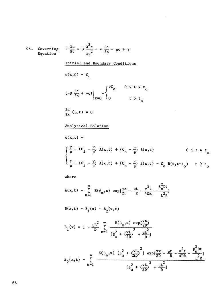
C8. Governing Equation
„ ac ^ 3^c ac '^ at = ^ ^^2 - ^ 3x - ^'^ -^ ^
Initial and Boundary Conditions
c(x,0) = C,
vC
(-D |£ H- VC) x=0 ^0
0 < t < t
t > t
If (L'^)=0
Analytical Solution
c(x,t) =
Í+ (Ci-^) A(x,t) + (C^-^) B(x,t) 0 < t < t
^+ (Ci --J) A(x,t) + (C -^) B(x.t) - C B(x.t-t ) o p' t > t
where
vx A(x,t) = I E(ß^,x) exp[2p m=l R 4DR
2
B(x,t) = B^(x) - B^ix.t)
Bj(x) = 1 UL 2 « E(ß^,x) exp(g)
D ^ 2 2 ">=! fg2 + Ä + ^'L 1
B2(x,t) = I B(3„.x)l3f.(^)]exp[||-^-|^ m m
L2R
in=l 2 2
^^m ^ 4D^ D ^
66
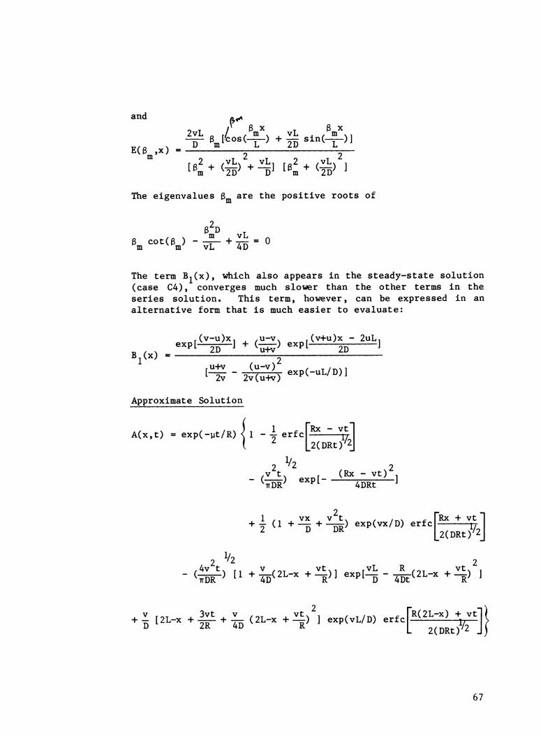
and p^^ o T /^ ß X - ß X
2Xilß r/eo8(-^)+|^sin(-^)] E(3^,x) =-^_^ ^ 2D L__
The eigenvalues ß are the positive roots of
2 ß D
, V m vL ß cot(ß ) - -^r— +-^ = 0 m m vL 4D
The term B,(x), which also appears in the steady-state solution (case C4), converges much slower than the other terms in the series solution. This term, however, can be expressed in an alternative form that is much easier to evaluate:
r(v-u)x, , /U-Vv r(v+u)x - ZuL, , , , ^^P[-2D-^ ^ ^-^^ ^^Pt 2D ^ B^(x) = 2
rU+V (U-V) . T/^v1
Approximate Solution
A(x,t) = exp(-pt/R) < 1 1 crfcf'^ " ^w1 2 [2(DRt/'^2j
2 ^/2 2 ,v t. r (Rx - vt) ,
- (¥DR> ^^Pt äDRT—J
2 + |- (1 + ^ + ^) exp(vx/D) erfc
L2(DRt)'2j
2 '/2 2 /^V tv r, . V ,^_ . Vt., rVL R /OT J Vt. ,
- (lÍDR-> fl + 4D^2L-x H-^)] exp(^ - ^(2L-x + _) ]
+ ^ [2L-X +|ïi + ^ (2L-X +^) ] exp(vL/D) erfc [R(2L-x) + vt"jl 2(DRt//2 Jl
67

B(x,t) « B2(x,t)/B^(x,t)
where
r. / N V .(v-u)xi - [EX - utl
<^-"> 2D L2(DRtr2j
l^D D R L 2(DRt)/2 J
3 Vo 2 - :îL_ (_L.) exDl— -^ - -^(2L-x + ^) 1
. _vf rV(2L-x) .A 2(iD ^ D DR
+
|j,D TtDR
v(u-v) r(v+u)x - 2uL r(v+u)x - 2uL, ._^.rR(2L-x) - utl
(.u+vy ^ L 2(DRt)^2 J
v(u+v)
(u-v)^
r(v-u)x + 2uL, - r R(2L-x) + ut] exp[ 20 ^ ^^^'^X 7h~ ^" L 2(DRt)^2 J
Í - ^2 B, (x) = 1 - *-" "^^ exp(-uL/D)
^ (u+v)^
and
u = V (1 + ^) V
V2
68
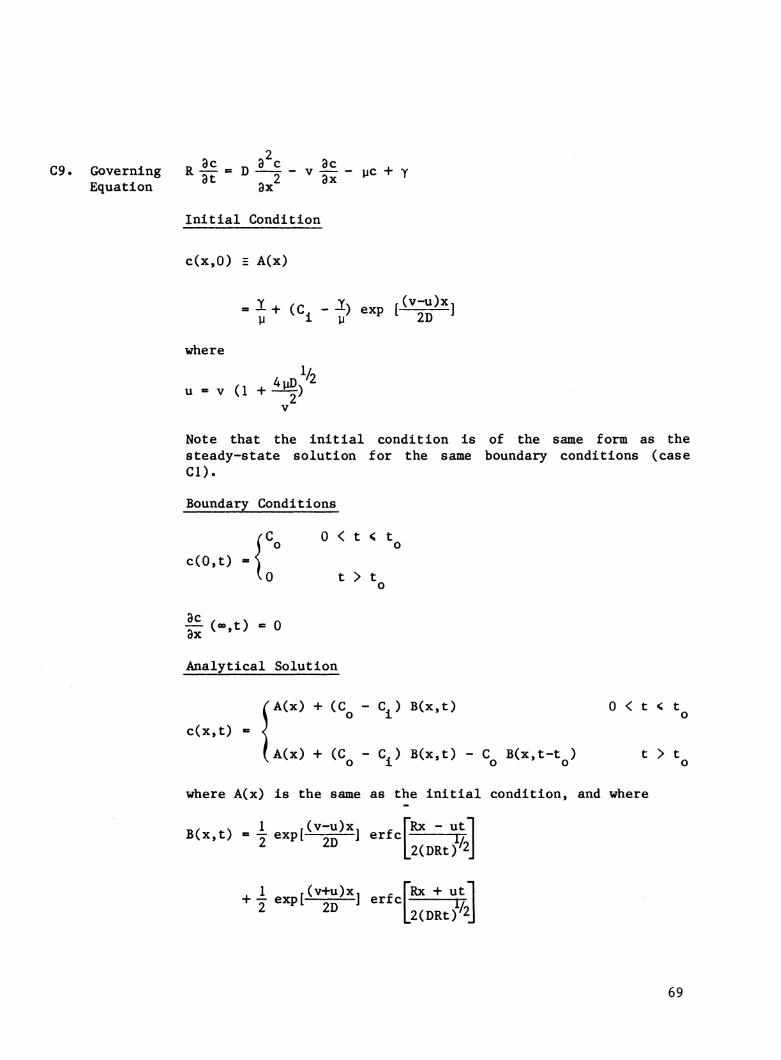
C9. Governing R |^ « D ^ " ^ |j " 1^^ + y Equation 3x
Initial Condition
c(x,0) = Ä(x)
= í*«=l- where
u « V (1 V
(v--u)x, 2D ^
Note that the initial condition is of the same form as the steady-state solution for the same boundary conditions (case Cl).
Boundary Conditions
(C 0 < t < t j o o c(0,t) =<
^0 t > t o
t(-,t).o
Analytical Solution
c(x,t)
A(x) + (C - C ) B(x,t) 0 < t < t
A(x) + (C - C^) B(x,t) - C B(x,t-t ) t > t o ^^ -< 9 y oo o
where A(x) is the same as the initial condition, and where
B(x,t) = j exp[—2D—1 ®rf^
. 1 r(v-hu)x, ^ 1 ^^Pt 2D -*
[Rx - uti 2(DRt?2j
L2(DRt)^2j
69

2 CIO. Governing R |f = D -^ - v -f^ - yc + y
Equation 8x
Initial Condition
c(x,0) E A(x)
Y . /r. Y\ 2v r(v-u)xi
where
V9
V V
Note that the initial condition is of the same form as the steady-state solution for the same boundary conditions (case C2).
Boundary Conditions
/vC^
(-DH+VC) =< ^"^ x=0 (0
0 < t < t 0
t > t 0
II (..t) . 0
Analytical Solution
c(x,t)
'A(X) + (C - C.) B(x,t) 0 < t < t 01 o
A(x) + (C - C^) B(x,t) - C B(x,t-t ) t > t
where A(x) is the same as the initial condition, and where
L2(DRt)^2j
[Rx + ut"|
2(DRt?y
,vx utv j, FRX + vt"] exp(— - -^) erfc jy
° ^ L2(DRt)/2j
V f(v+u)xi £
2
70

cil. Governing R||-=D^-v||-yc + Y Equation 9x
Initial Condition
c(x,0) = A(x)
where
r(v-u)x, , /U-v. ,(v+u)x - 2uL, - 1 + (C 1) ^^P^~2D-J -^ ^^^ ^^P^ 2D ^
"^ ' ^ [l + (^) exp(-uL/D)]
V2 u = V (1 + A!|)
V
Note that the initial condition is of the same form as the steady-state solution for the same boundary conditions (case C3).
Boundary Conditions
c(0,t) =
C 0 < t < t o o
\0 t > t o
Analytical Solution
A(x) + (C^ - C^) B(x,t) 0 < t < t^
c(x,t)
.A(x) + (C - C^) B(x,t) - C B(x,t-t ) t > t o 1 00 o
where A(x) is exactly the initial condition, and where
B(x,t) = B^(x) - B^Cx.t)
with
71
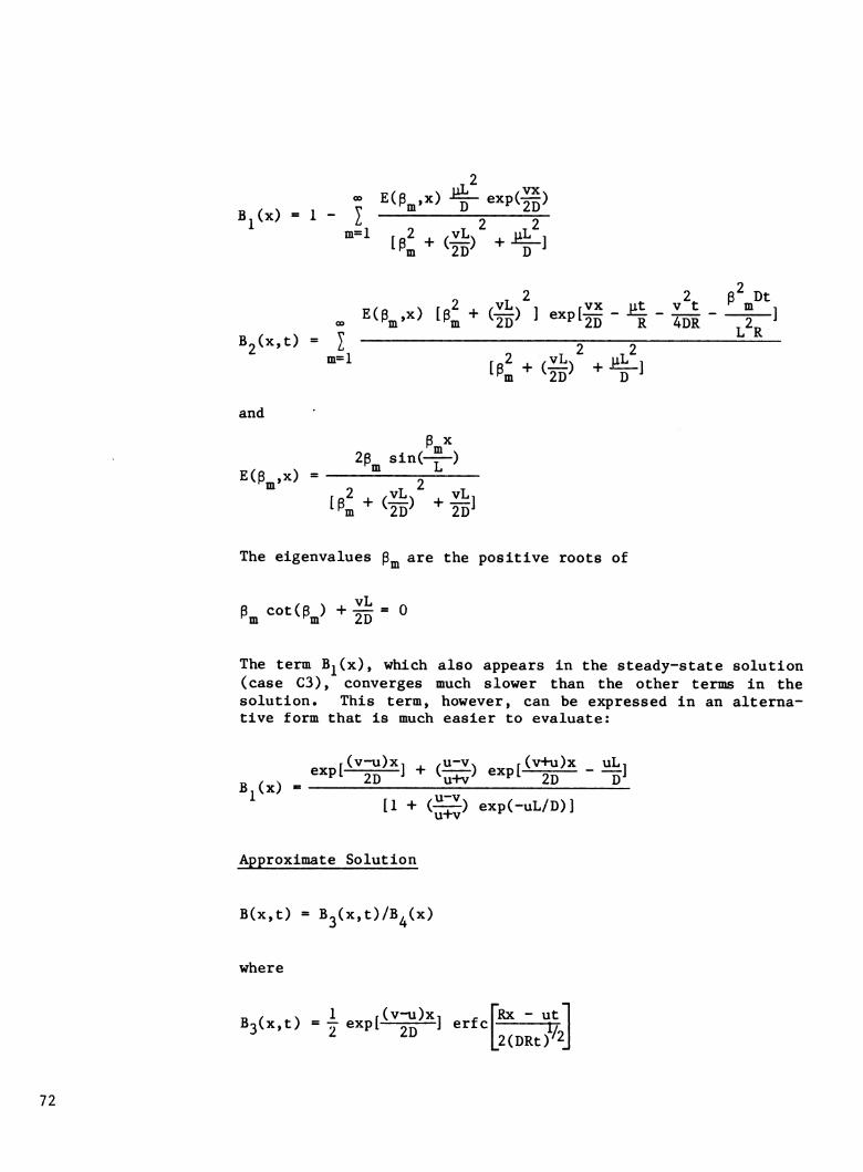
B^(x) = 1-1 2 2~
9 T 2 ^ 2^ ß^ Dt » E(ß^.x) Iß^ + (^) ] exp[^ - ü^ - _ - ]
B^Cx.t) = l 2 2 ^^
and
2p„ sIn(-J!-)
The eigenvalues ß^^^ are the positive roots of
ßm^°^^ßm^ ■'lïï-O
The term Bj^(x), which also appears in the steady-state solution (case C3), converges much slower than the other terms in the solution. This term, however, can be expressed in an alterna- tive form that is much easier to evaluate:
r(v-u)x, . /U-Vv r(v-Ki)x ULi
^ , , ^^Pt-2^^ ^ ^^^ ^^P^-2D pJ B (x) « [1 + (^) exp(-uL/D)]
Approximate Solution
B(x,t) = B2(x,t)/B^(x)
where
BjCx.t) - I exp(iïg^l erfc L2(DRt)'2j
72

. 1 r(v+u)x, ^ FRX -h Utl
v^ rVL ut, , rR(2L-x) + vtl -=r exp -fT - -^] erf c -i ij— ^"^ "^ ^ L 2(DRt)/2 J
B^(x) = 1 + (^) exp(-uL/D)
73
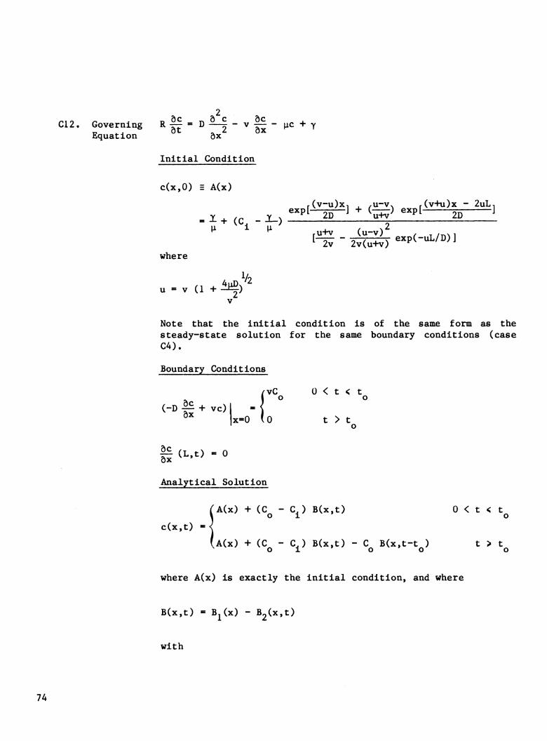
2 C12. Governing í^|f=í^-^-v|f- Jic + y
Equation ôx
Initial Condition
c(x,0) = A(x)
f(v-u)x, , /U-v. f(v+u)x - 2uLi
= X + (c - X_) ^^P^~lD~^ "^ ^^^ ^^P^ 2D J
^ ^ rU+V CU-V) f T /TN\ 1
where
V
Note that the initial condition is of the same form as the steady-state solution for the same boundary conditions (case C4).
Boundary Conditions
!vC Ü < t < t o o
.0 t > t o
H ^^-^^ - " Analytical Solution
c(x,t)
A(x) + (C^ - C^) B(x,t) 0 < t < t
,A(x) + (C^ - C^) B(x,t) - C^ B(x,t-t^) ^ '* ^o
where A(x) is exactly the initial condition, and where
B(x,t) = Bj(x) - B2(x,t)
with
74

.2
Bj(x) = 1 - ¿ 2 T
T-/0 \ r,,2 . /VL. , fVX Lit V t m 1
B^Cx.t) = ^ 2 2 ™=1 r«2 . .vL. . LlL 1
ißm + %> -^ D 1
and
The eigenvalues ß^^ are the positive roots of
E(ß„,x) =
'^m . vL ß cot(ß ) - —r + TT: = 0 ^m ^m vL 4D
The term B^Cx), which also appears in the steady-state solu- tion (case C4), converges much slower than the other terms in the series solution. This term, however, can be expressed in an alternative form that is much easier to evaluate:
r(v-u)x, . /U-Vv r(v-Ki)x - 2uLi , , , ^^pt-2ïr-i "^ ^^^ ^^pt 2D ^ B,(x) =
rU+V (U-V) f T /TAM
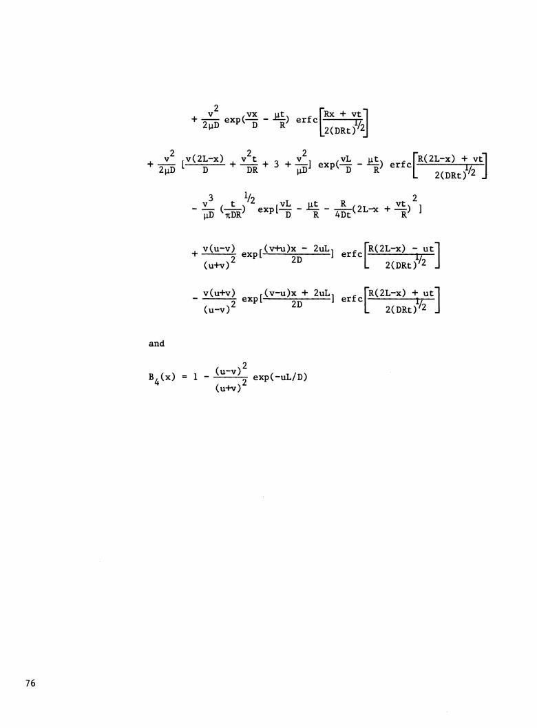
Approximate Solution
B(x,t) = B2(x,t)/B^(x,t)
where
Ti ( ^\ V r(v-u)x, ^ TRX - ut"|
V r(v-Ki)Xi ^ FRX + utl
75
2 , V ,VX lit, ^
^ 2¡lD ^^P^-D - R^ "^'^
V rV(2L-x) . V t , ^ . V 1 .VL LLtv -
L2(DRt)'2j
[R(2L-x) + vt] 2(DRt)^2 J
V , t . ^ fVL ut R /OT j. vt. , - TiD ^xDR> ^^P^-^ - R - 4DF^2L^ + —) ]
. v(u-v) r(v+u)x - 2uL, j. I + —^^ 5" exp[-^ '-— 1 erfc (u+v)^ ^" L 2(DRt)'
v(u+v) r(v-u)x + 2uL, ^ 3 ^'^Pl 2D ^ ^^^^ (u-v)
rR(2L-x) - ut"| L 2(DRt)^2 J
[R(2L-x) + ut"! 2(DRt)^2 J
and
.2 B (x) = 1 - -^ii=^ exp(-uL/D)
(u+v)^
76

C13. Governing R 1^ = D ^ - v |^ - HC + Y T-i ^j ot ^ z ox Equation ox
Initial and Boundary Conditions
c(x,0) = C^
c(0,t) = C + C, e"''^ a D
If (-.t) - 0
Analytical Solution [see Cleary and Ungs ( 1974 ) and Marino (1574b) for some special cases]
c(x,t) = ^ + (C, - ^) A(x,t) + (C^ - ^) B(x,t) + C, E(x,t)
where
A(x,t) «= expf^it/R) |l - j erfc]^ " "g 1 ( ^ L2(DRt)^2j
- -r- exp(vx/D) erfc \T > 2 L2(DRt)/2j )
B(x,t) = T; exp[^ ^/ ] erfc jr L2(DRt)'2j ^ e.pl-^, -'=fc^
^ 1 r(v4-u)xT - 2" ^^^ "20—^ L2(DRt)'2j
r./- ^^ ~^t» 1 f(v-w)Xi ^ FRX-Wtl
[Rx + wtl )
.2(DRt)'/2j ] . 1 r(v-h^)xT ^
"2 ^^^'—2D—^
and with
77

u = v (1+-^) V
V2
w = V [1 +^i\i - \R)] V
V2
78

C14. Governing ^ ff " ^ ^ " ^ fs " »^^ "*" ^ Equation ox
Initial and Boundary Conditions
c(x,0) = C,
(-D II + vc)
ë <-'' - °
= v(C + C^^e"'^'^) n ab x=0
Analytical Solution (see also Lindstrom and Oberhettinger 1975)
c(x,t) =
^+ (C, -^) A(x,t) + (C - ^) B(x,t) + C, E(x,t) i[i * XR)
^ + (C, - C, - ^) A(x,t) + (C -^) B(x,t) + C.e"^*^ ((x = \R) Hibp, an b
where
A(x,t) = exp(-|it/R) { 1 - 1 erf r^ " "^.^1
V2 2 ^ 2 ,v t. r (Rx - vt) ,
. (—) exp[ 45R^—1
2
+ T (1 +^ + ^) exp(vx/D) erfcl^i^^ 2 ^ ^^ l2(DRtf2
JMJL L2(DRt
B(x.t) = i-;^) exp[Í5^] erfc
. / V V r(v-»-u)Xi r:
L2(DRt)'2j
L2(DRt)^2j
79

^2 ^^ ^
L2(DRt)'2j
u ^\ _ „"^»•t)/' V X r(v-w)xi £ PRX - wtl
[Rx + wtl )
2(DRt//2j ) . / V V r(V+W)X, ^ + (^) exp[-2Ö-] erfc
and
u = V (1 + -^) V
4D ^/2 w = V [1 +-=^(ti - \R)]
V
80

C15. Governing l^|f=D^-v|j-iiC + Y Equation ox
Initial and Boundary Conditions
c(x,0) = C^
c(Ü,t) = C^ + C^^ eT^^
If (^'^> = ' Analytical Solution
c(x,t) =
^+ (C -^) A(x,t) + (C -^) B(x,t) + C, F(x,t) {[X t XR) ^i i |i a |i b
^ + (C - C^ - ^) A(x,t) + (C - ^) B(x,t) + C. e"''^ (^i = \R) |i i b p. Û ^ b
where
^2^ ß^Dt w N VT.fr. \ rVX lit vt nil A(x,t) = I E(ß^.x) expl^ - J±_ - ^^ - ]
IIl~l ij K
B(x,t) = B^(x) - B2(x,t)
2 - E(ß„.x) ^ exp(||)
Bj(x) =1-1
""' Ie^<3>'-^1
2 L ^ vx t v^t ^m^*^ » E(ß^.x) [ß^ + (f^) 1 exp[|f - ü^ - |j^ - -^]
B2(x,t) = I 2 2
^Pm ^ 4D^ D ^
81

F(x,t) = e"^*" [Fj(x) - F2(x,t)]
F l(x) = 1-1
2
~ ^(^m''^^ D ^^P^lD^
m=l .2 ,vL.^ (ti - XR)L^. ^^m ^ %^ + D J
2 2 2 ß Dt
V''> ' Î 2 2 ^"-^ and m 2D D
6 X 23^ 8in(^)
E(3„,x) " ^
^^^<i)'-Iü^
The eigenvalues ß are the positive roots of
^ ^°^(^> -^ il = 0
The terms B^Cx) and F^Cx) converge much slower than the other terms in the series solution. Both B^(x) and F^(x), however, can be expressed in alternative forms that are much easier to evaluate (case C3):
^ ^r(v-u)xi , /U-Vv r(v+u)x - 2uLi R r ^ exp[-^g-] + (^ exp[ ^ ] B (x) =
[1 + (^) exp(-uL/D)l
^„„r(v-w)x, , /W-Vv f(v+w)x - 2wL, F (X) = ^^-^P-J + <^ ^^Pt 2B J
^ [1 + (^) exp(-wL/D)]
where
u = V ( 1 + —^) V
V2
82

4D '/2 w = V [1 +^(|i - \R)]
V
Approximate Solution
[Rx - vtl A(x,t) = exp(-(it/R)<l - -^ erfc
1 / /T.N ^ TRX + vtl ■ -y exp(vx/D) erfc jj ^ L2(DRt)^2j
¿t 2 '" ■ D 'DR' 1 f„ . v(2L-x) . V t, ,- T /n^ Í rR(2L-x) + vt1 -T 12 + f^ + -f^] exp(vL/D) erfc n—
L 2(DRt)^2 J
2 '/2 2 . /V tx rVL R /OT -i_ Vtx 1 ■^ ^^^ ^^Pi-D- 4DF^2L-X+—) ]
B(x,t) = B2(x,t)/B^(x)
where
„ , ^. 1 r(v-u)x, £ FRX - ut"| B (x,t) =-=■ expl—^T-—] erfc n;
. 1 ,(V+U)XT „ FRX + ut"| ■*" 2 ^^Pt 2D ^ ^'"^'^ 1/9
^ (u-v) r(v+u)x - 2uL, ^^,^ rR(2L-x) - ut1 + T7::Z;TT expl ^^^ J erfc rr
L 2(DRt)'2 J Tü+v) ""^^ 2D"
^2 (u+v) ,(v-u)x + 2uL, ^ rR(2L-x) + utl
2-^ -P<^ - ^^ "i^l ,,„^^, rR(2L-x) + vtl L 2(DRt)^2 J
83

rU-Vx ^4^""^ " ^ "^ ^i+7^ exp(-uL/D)
and
F(x,t) - e"'^'' F3(x,t)/F^(x)
where
F3(x.t) = i exp[i3^] erfcP^Í^-:i-SÍt' :3vx,ty = Y expi—20"
, 1 r(V+W)Xi - "2 ®^Pl 2D ^
L2(DRt)'2j
["RX + wtl
+ _(wil). ^,pr(v+w)x - 2wL, ._,JR(2L-X) - wt1 * 2(w+v) ^Pl 2D ^ "^^ : 1^— L 2(DRt)'2 J
-. (w+v) ,(v-w)x + 2wL, ^ rR(2L-x) + wtl
2 - V «^„/-vL M X ^^^ t rR(2L-x) + vtl ___ exp(- - \ + Xt) erf c[——T^J
F^(x) - 1 + (^) exp(-wL/D)
84

2 C16. Governing R -5— = D —^ - v -5— - yc + y
„ ^ . ot ,. Z ox Equation 9x
Initial and Boundary Conditions
c(x,0) = 0
(-D|^+ VC)| = v(C + C. e ^^) 3x ^ a b x=0
t (^■"=° Analytical Solution
c(x,t) =
^ + (C- I) A(x,t) + (C - I) B(x,t) + C, F(x,t) (u * XR) pip a p D
1 + (C- C, - I) A(x,t) + (C - I) B(x,t) + C, e"'^*' (y = XR) y 1 D )j ay D
where
^2^ ß^Dt w \ V T./0 N fVx yt V t m 1 A(x.t) = I E(3^,x) exp[^ -_-_-]
m=l L R
B(x,t) = B,(x) - B,(x,t)
» E(ß* ,x) ^ exp(^) Bi(x) = 1-1 -^5 5_ 2D_
m=l roZ .vL. yL ,
o T 2 ,2^ ß^Dt 17/o \ ro2 . .vLv , rvx yt V t m ,
« ^(^'^> f^m -^ %^ Í ^^Pt2D - -R - 4DR - -^^ B^Cx.t) = I 2 2
85

F(x,t) = e'-^'^LFjíx) - F^íx.t)]
F ̂(x) =1-1
2
'% "^ W "^ D
2 2 ß^Dt
ri Li K F (x,t) = I 2 2
■"=! [«2 . ^VL/ (y - XR)L ,
and
ß X ^ ß X ß_ [ß_ cos(-^ï-) + C-^r^) sin(-=—)] „,„ - D m ^"^m ^ L ' 2D' L
E(ß ,x) = ^ j-
The eigenvalues ß are the positive roots of m
ß^D ^
The terms B,(x) and F,(x) converge much slower than the other terms in the series solution. Both B^ix) and F^Cx), however, can be expressed in alternative forms that are much easier to evaluate (case C4):
B,(x) exp[<Ig)£j . (^) exp[<-^">- ^"^]
1 2 rU-HV (U-V) . - /-v ,
exD (^~^)^ + (2î::l) expí-^3^tí^^^^_2í5;i exp + í.^^; expi 2D [ F (x) = 2
,/W+V. (W-V) , T /T^^ 1
where
86

V
. 4D ^/2 w-vll+-í|(p- XR)]
V
^proximate Solution
A(x,t) exp(-pt/R) <1 - Y i ^.j.f TRX - vtl
2 ^'^ ""UCDR^J \
_ (¿t^ (Rx - vt)^ ''TTDR'' ^"^^ 4DRt J
L2(DRt)'2J
2 '/2
T - 4DF(2L-X + —) ]
-^ ÏÏ f2L-x + Ü^ + ^2L-x + :|)'] exp(vL/D) erfoF^^iL-^ L 2(DRt)
vt w B(x,t) = B2(x,t)/B^(x,t)
where
[ÍRX + utl
2(DRt?2j
[Rx + vt"|
2(DRt?y
. V r(v+u)x,
, V ,VX lit. D R
.2. 2 + JL. r^(2L-x) + v_t v_ vL _ pt ,_^.rR(2L-x) + vt1
L 2(DRt)'2 J
87

- -^ (;;ïï^> ^^P^ D R 4Dt^ R yD irDR
, v(u-v) ,, .iZÍHli-JHÍi] erfc^Mli=^^^f| + :i ^''P^ 2D L 2(DRt)'2 J
(u+v)
72 ® P^ 2D L 2(DRt)'2 J (u-v)
B (X) - 1 - -^ exp(-uL/D) 4 (u+v)^
and
F(x,t) - e"^^ F (x.t)/F^(x)
where
F3( X.C, . C^) «XP.^^1 «-g¿¡S
¿ ^ TRX + vt I v^ _„^vx _ JMt + ^t) erfc - 1/
L2(DRt)^2J ■^ züñFm ""P^"^ " "^
v^ ,v(2L-x). ^ ¿t - ^ .YI
i- FRCZL-X) 4- vt"l
2 ) 1
D(y-XR) TTDR
88

vÇwzvl e,pt(v4^)x - 2wLj ^^^ rR(2L-x) - wtl (wfv)2 2D L 2(DRt)/2 J
(w-v)2 2D L 2(DRt)'2 J
( ^2 F, (x) - 1 - -i^Î=^ exp(-wL/D)
^ (wfv)^
89

5. EFFECT OF BOUNDARY CONDITIONS
In this section we will present several calculated solute distributions as a function of distance and time. Special attention will be given to the effects of the applied upper and lower boundary conditions. The results are generalized by making use of the following dimensionless variables
P = vL/D T = vt/L z = x/L [14]
where P is the column Peclet number, T is the number of dis- placed pore volumes, and z is the reduced distance. To make the solutions for a semi-infinite system applicable to a finite profile of length L (for example, a laboratory soil column), the reduced distance cannot exceed one (0 < x < L).
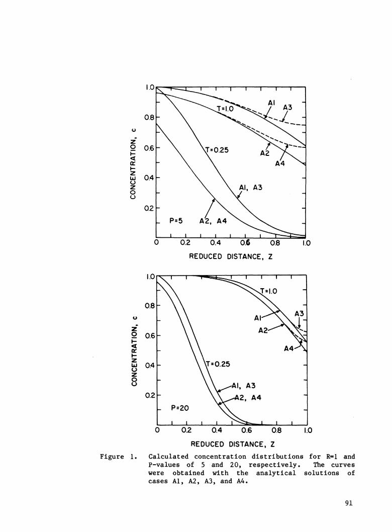
Figure 1 shows calculated distributions obtained with the solutions of cases Al (first-type boundary condition at x = 0; semi-infinite profile), A2 (third-type boundary condition; semi-infinite profile), A3 (first-type boundary condition; finite profile), and A4 (third-type boundary condition; finite profile). Results are given for P-values of 5 and 20, and at times equivalent to displaced pore volumes of 0.25 and 1.0. The retardation factor (R) is assumed to be one; by replacing T by T/R, the curves in figure 1 also hold for values of R other than one. Furthermore, the curves are for no production and decay (y = ^1 = 0), for an initial concentration (C^) of zero, and for a continuous input concentration (C^) of one.
A considerable effect of the upper boundary condition on the results is apparent at a Peclet number of 5. The curves for a first-type boundary condition (cases Al and A3) are much higher than those for a third-type boundary condition (A2, A4) throughout the entire profile. The curves for a semi-infinite system (Al, A2), furthermore, are very similar to those for a finite system (A3, A4) at relatively small times (T < 0.25 in fig. 1). This similarity occurs when the solute fronts are still not influenced by the lower boundary. Large differences between the solutions for a finite and semi-infinite system, however, are present at later times. These differences are greatest after about one pore volume. When P increases from 5 to 20, the differences between the various solutions become much smaller. Note that for P = 20 the solutions for a finite and semi-infinite system deviate from each other only in a very small region near the lower boundary.
From a large number of comparisons we found that the solution for a finite system can be approximated with an accuracy of at
90
1.0
0.8-
9 0.6
er
u 0.4 o z o o
0.2"
^
lili
>4" - \ V=0.25 A2 /\ '
" \ A4 \
- Al, A3
- P=5
1 1
A2, A4
1 1 1 \^^^^
0.2 0.4 0.6 0.8
REDUCED DISTANCE, Z
1.0
REDUCED DISTANCE, Z
Figure 1. Calculated concentration distributions for R=l and P-values of 5 and 20, respectively. The curves were obtained with the analytical solutions of cases Â1, A2, A3, and A4.
91

least four significant places by solutions for a semi-infinite system as long as z is restricted to
0 < 2 < .9 - 8/P. [15]
This empirical rule, which holds for all values of T, applies also for cases where production or decay terms are present. For relatively small values of T (for example, for T less than 0.25 in fig. 1), [15] could be expanded to a much larger part of the profile.
Except for the region close to the column entrance, the largest differences between the four solutions occur at the lower boundary after about one pore volume. Figure 2 shows the effect of P on the lower boundary concentration at T = 1 for the four analytical solutions. The curves diverge considerably from each other at the lower Peclet numbers. The curves for Al and A4 approach each other slowly when P increases; at a Peclet number of 10, the difference is only 0.05 unit. The curve for A2, although always less than 0.5, converges to 0.5 rather quickly; it reaches a value of 0.493 at P = 10.
Differences among the various analytical solutions, such as those shown in figure 2, are important. Estimates of the coefficients P and R in the transport equation are often obtained by fitting one of the analytical solutions (Al to A4) to observed column effluent data (van Genuchten 1980). This procedure assumes that the exit concentration can be equated to the concentration at the lower boundary.
Although considerable differences between the analytical solutions are present, even at Peclet numbers as high as 100 to 200, the significance of these differences are somewhat mis- leading when judged from figure 2 alone. This is because of the increasingly steeper slope of the exit concentration when plotted against T. This effect is shown in figure 3, where effluent curves are given for Peclet numbers of 5, 20, and 60. Figure 3c shows that only a small displacement is needed to let all solutions converge to the same curve (P = 60). The maximum differences between the curves in figures 3b and 3c, furthermore, are roughly of the same order of magnitude as the experimental errors one may expect in carefully obtained effluent curves. It seems likely, therefore, that the effects of the imposed mathematical boundary conditons can be neglected when P reaches values of about 20 or 30.
Two additional observations follow from figure 3. First, the effluent curves for cases Al and A4 are very close when P is about 5 or higher. This property was demonstrated earlier by
92

Figure 2. Effect of P on the concentration at x = L and for T = 1. The curves were obtained with the analyt- ical solutions of cases Al, A2, A3, and A4.
0.4 08 1.2 \4 2.0 ZA
PORE VOLUME, T
08
H 04
02-
—r 1 1 1 1 1 1 '^^^i^*''^^ ' 1
" /óy - B
'// -
11 _ ///^Al. A4
- II - - I - - I -
L -L^ ¿1-. J- i 1 > 1 i 1 1
-
0.4 Oß 12 I 6 2 0 2 4
PORE VOLUME, T
08
2 0.6-
z ui 04 •i O
02
-T 1 1 1 1 r
P«60
J I UW I I I I L_ I I I L 04 08 \z Te 2^0 ZÄ
PORE VOLUME. T
Figure 3. Effect of P on calculated effluent curves for cases Al, A2, A3, and A4.
93

Parlange and Starr {1975 ). The errors introduced by approx- imating the solution of A4 by the much simpler solution of Al are about the same as the differences between the curves Al and A4 in figure 2. Second, the curves for Al in figure 3 are located exactly between those for A2 and A3. In equation form this can be expressed as
^A3 = 2c^i - CA2 (^=L) [16]
where the subscripts Al, A2, and A3 refer to the appropriate analytical solutions. This last property, which is extremely accurate for values of P that are not too small, follows directly from the approximate solution of case A3. Similar relations apply for all approximate solutions for a finite system and a first-type boundary condition at x = 0 (that is, also for nonzero values of \, ^i, and y). For example, for case C7 one has
^C7 ' 2cc5 - c^^. (x=L) [17]
The above discussion of the boundary effects is restricted to cases where the production and decay terms are zero. Similar effects of the boundary conditions can also be demonstrated when either y» M-» or both are nonzero. Only a few comments for these cases will be given here. The effects of the boundary conditions are generally more pronounced for the special case of zero-order production only (y ^ 0, ^L = 0). This is shown in figure 4 where the steady-state solutions of cases Bl to B4 are plotted for two values of the column Peclet number. Results are given for C = 1 and a value of one for the dimensionless rate term
Y » yL/v. [18]
The differences between the four solutions are considerable, especially when P equals 5. Note that the solution for case Bl is independent of P.
The effects of the boundary conditions are generally less significant when, in addition to zero-order production, the chemical is also subject to first-order decay. Figure 5 shows the steady-state solutions of cases Cl to C4, for two values of y, and for a value of one for the dimensionless decay constant
Il = ^lL/v. [19]
The curves for the two values of y are, in this particular example, sjnmnetric with respect to the line c = 1. Note that.
94

02 0.4 0.6 0.8 1.0
REDUCED DISTANCE, Z
Figure 4. Effect of P on steady-state concentration distributions for cases Bl, .B2, B3, and B4,
1.6
•2-
i .(
Ö 0«
06
04-
02-
- T IT T— I I 1 1 I
_ C2 ^ ̂ ;;^^^^^\ - \^^ _
y yy^ /•2
' y^ -
< yc\ -
xT - N N/\. X-o
- I^\^^v^ - - C2 ^\^ \:>;4-.; - ^^**^§< - C4
- P«5 _
- lili -L. .± _._! 1-, 1
Ü
1.6
T V 1 ■ T ■ -T r T ■ -r- - I
1.4 : . .^^^^^^^ _
C2 yy^^ -
12
yy -
1.0 x' -
08 /\v -
- C2 \X^ -
0.6 : ^ ̂ ^v^^.O -
0.4 - ==^
0.2 P«20
1 1 1 1 1 1 1 1 L.
0 02 04 0.6 OB 1.0
REDUCED DISTANCE. Z
02 04 06 Oß 1.0
REDUCED DISTANCE, Z
Figure 5. Effect of P on steady-state concentration distributions for cases Cl, C2, C3, and C4.
95

at a Peclet number of 20, the finite and semi-infini te solu- tions are essentially the same over the region 0 < z < 0.95. The effects of the boundary conditions are generally more pronounced when the ratio y/p increases; the effects are relatively small when y = 0 and y is large.
6. NOTATION
S3anbol Definition
c Solution concentration.
^Al» ^A2* ^A3 Effluent concentrations based on the solu- tions of cases Al, A2 and A3, respectively.
^C5» ^C6> ^C7 Effluent concentrations based on the solu- tions of cases C5, C6, and C7, respectively.
Cj^, C2 Constants in several initial conditions (table 1).
C^, C^ Constants in several boundary conditions (table 1).
C^ Initial concentration (table 1).
CQ Input concentration (table 1).
D Dispersion coefficient.
f(x) General initial condition.
g(t) General input concentration.
k Distribution constant.
L Column length.
P Column Peclet number (P = VL/D).
q Volumetric flux.
R Retardation factor (R = 1 + pk/e).
S Adsorbed concentration.
t Time.
t Duration of solute pulse (table 1).
96

u
Pore volume (T = vt/L).
Y Pore-water velocity,
w w = [v^ + 4D(^-\R]'^2
X Distance«
Xj Constant in several initial conditions (table 1).
y y » (v - ^\mr^.
z Reduced distance (z = x/L).
a Decay constant in several initial conditions (table 1).
ß m-th eigenvalue«
Y General zero-order rate coefficient for produc- tion.
Y Zero-order solid phase rate coefficient for production.
Y Zero-order liquid phase rate coefficient for production.
Y Dimensionless zero-order rate coefficient (Y = Y^/v).
9 Volumetric moisture content.
\ Decay constant in several boundary conditions (table 1).
\x General first-order rate coefficient for decay.
|i First-order solid phase rate coefficient for decay.
|i First-order liquid phase rate coefficient for decay.
¡I Dimensionless first-order rate coefficient (í¡ = ^iL/v).
p Bulk density
97

7. LITERATURE CITED
Abramowitz, M., and Stegun, I. A. 1970. Handbook of mathe- matical functions. Dover Publications, New York.
.Arnett, R. C, Deju, R. A., Nelson, R. W., and others. 1976. Conceptual and mathematical modeling of the Hanford groundwater flow regime. Report No. ARH-ST-140, Atlantic Richfield Hanford Co., Richland, Wash.
Baron, G., and Wajc, S. J. 1976. Thermal pollution of the Scheldt estuary. In; G. C. Vansteenkiste (editor). System simulation in water resources, North-Holland Publishing Co., Amsterdam, p. 193-213.
Bastian, W. C, and Lapidus, L. 1956. Longitudinal diffusion in ion exchange and Chromatographie columns. Finite column. Journal of Physical Chemistry 60:816-817.
Bear, J. 1972. Dynamics of fluids in porous media. American Elsevier Publishing Co., New York.
— — — 1979. Analysis of flow against dispersion in porous media - Comments. Journal of Hydrology 40:381-385.
Brenner, H. 1962. The diffusion model of longitudinal mixing in beds of finite length. Numerical values. Chemical Engi- neering Science 17:229-243.
Carslaw, H. S. and Jaeger, J. D. 1959. Conduction of heat in solids. Second edition. Oxford university Press, London.
Cleary, R. W. 1971. Analog simulation of thermal pollution in rivers. In: Simulation Council Proceedings l(2):41-45.
— — — 3jj¿ Adrian, D. D. 1973. Analytical solution of the convective-dispersive equation for cation adsorption in soils. Soil Science Society of America Proceedings 37:197- 199.
— — — 3^¿ Ungs, M. J. 1974. Analytical longitudinal dis- persion modeling in saturated porous media. Summary reprint of paper presented at the Fall Annual Meeting of the American Geo- physical Union, San Francisco.
DiToro, D. M. 1974. Vertical interactions in phytoplankton — An asymptotic eigenvalue analysis. Proceedings of the 17th Conference, Great Lakes Research, International Association Great Lakes Research, p. 17-27.
98

Duguid, J. 0., and Reeves, M. 1977. A comparison of mass transport using average and transient rainfall boundary con- ditions. J[n W. G. Gray, G. F. Pinder, and C. A. Brebbia (editors). Finite elements in water resources, Pentech Press, London, p. 2.25-2.35.
Gardner, W. R. 1965. Movement of nitrogen in soil. _rn W. V. Bartholomew and F. E. Clark (editors). Soil nitrogen. Agronomy 10:550-572. American Society of Agronomy, Madison, Wis.
Gershon, N. D., and Nir, A. 1969. Effect of boundary condi- tions of models on tracer distribution in flow through porous mediums. Water Resources Research 5:830-840.
Glas, T. K., Klute, A., and McWhorter, D. B. 1979. Dis- solution and transport of gypsum in soils: I. Theory. Soil Science Society of America Journal 43:265-268.
Jost, W. 1952. Diffusion in solids, liquids, gases. Academic Press, New York.
Kay, B. D., and Elrick, D. E. 1967. Adsorption and movement of lindane in soils. Soil Science 104:314-322.
Keisling, T. G., Rao, P. S. C., and Jessup R. E. 1978. Per- tinent criteria for describing the dissolution of gypsum beds in flowing water. Soil Science Society of America Journal 42:234-236.
Kemper, W. D., Olsen, J., and Demooy, C. J. 1975. Dissolution rate of gypsum in flowing groundwater. Soil Science Society of America Proceedings 39:458-463.
Lahav, N., and Hochberg, M. 1975. Kinetics of fixation of iron and zinc applied as FeEDTA, FeHDDHA, and ZnEDTA in the soil. Soil Science Society of America Proceedings 39:55-58.
Lapidus, L., and Amundson, N. R. 1952. Mathematics of adsorp- tion in beds. VI. The effects of longitudinal diffusion in ion exchange and Chromatographie columns. Journal of Physical Chemistry 56:984-988.
Lindstrom, F. T., Haque, R., Freed, V. H., and Boersma, L. 1967. Theory on the movement of some herbicides in soils: Linear diffusion and convection of chemicals in soils. Journal of Environmental Science and Technology 1:561-565.
— — — ^j^¿[ Boersma, L. 1971. A theory on the mass transport of previously distributed chemicals in a water saturated sorbing porous medium. Soil Science 111:192-199.
99

— — — ^j^¿ Ober he t tinger, ¥. 1975. A note on a Laplace transform pair associated with mass transport in porous media and heat transport problems. SIAM, Journal of Applied Mathe- matics 29:288-292.
Lykov, A. v., and Mikhailov, Y. A. 1961. Theory of energy and mass transfer. Prentice-Hall, Englewood Cliffs, N.J.
Marino, M. A. 1974a. Longitudinal dispersion in saturated porous media. Journal of the Hydraulics Division, Proceedings of the American Society of Civil Engineers 100:151-157.
— — — 1974b. Distribution of contaminants in porous media flow. Water Resources Research 10:1013-1018.
Mason, M. and Weaver, W. 1924. The settling of small parti- cles in a fluid. Physiological Reviews 23:412-426.
Melamed, D., Hanks, R. J., and Willardson, L. S. 1977. Model of salt flow in soil with a source-sink term. Soil Science Society of America Journal 41:29-33.
Misra, C, and Mishra, B. K. 1977. Miscible displacement of nitrate and chloride under field conditions. Soil Science Society of America Journal 41:496-499.
Ogata, A., and Banks, R. B. 1961. A solution of the differ- ential equation of longitudinal dispersion in porous media. U.S. Geological Survey Professional Paper 411-A, A1-A9.
Parlange, J. Y., and Starr, J. L. 1975. Linear dispersion in finite columns. Soil Science Society of America Proceedings 39:817-819.
— — — and Starr, J. L. 1978. Dispersion in soil columns: Effect of boundary conditions and irreversible reactions. Soil Science Society of America Journal 42:15-18.
Pearson, J. R. A. 1959. A note on the 'Danckwerts' boundary condition for continous flow reactors. Chemical Engineering Science 10:281-284.
Reddy, K. R., Patrick, Jr., W. H., and Phillips, R. E. 1976. Ammonium diffusion as a factor in nitrogen loss from flooded soils. Soil Science Society of America Journal 40:528-533.
Selim, H. M., and Mansell, R. S. 1976. Analytical solution of the equation for transport of reactive solute. Water Resources Research 12:528-532.
100

Shamir, U. Y., and Harleman, D. R. F. 1966. Numerical and analytical solutions of dispersion problems in homogeneous and layered aquifers. Report No. 89, Hydrodynamics Laboratory, Mass. Inst. Tech. Cambridge, Mass.
Thomann, R. V. 1973. Effect of longitudinal dispersion on dynamic water quality response of streams and rivers. Water Resources Research 9:355-366.
van Genuchten, M. Th. 1977. On the accuracy and efficiency of several numerical schemes for solving the convective-dispersive equation. ^n_ W. G. Gray, G. F. Finder, and C. A. Brebbia (editors), Finite elements in water resources, Pentech Press, London, p. 1.71-1.90.
— — —. 1980. Determining transport parameters from solute displacement experiments. Research Report No. 118, U.S. Salinity Laboratory, Riverside, Ca.
— — —. 1981. Analytical solutions for chemical transport with simultaneous adsorption, zero-order production and first- order decay. Journal of Hydrology 49:213-233.
— — — and Wierenga, P. J. 1974. Simulation of one-dim- ensional solute transfer in porous media. New Mexico Agri- cultural Experiment Station Bulletin No. 628, Las Cruces.
— — — Qj^¿ Gray, W. G. 1978. Analysis of some dispersion corrected numerical schemes for solution of the transport equation. International Journal of Numerical Methods in Engineering 12:387-404.
Wehner, J. F., and Wilhelm, R. H. 1956. Boundary conditions of flow reactor. Chemical Engineering Science 6:89-93.
101
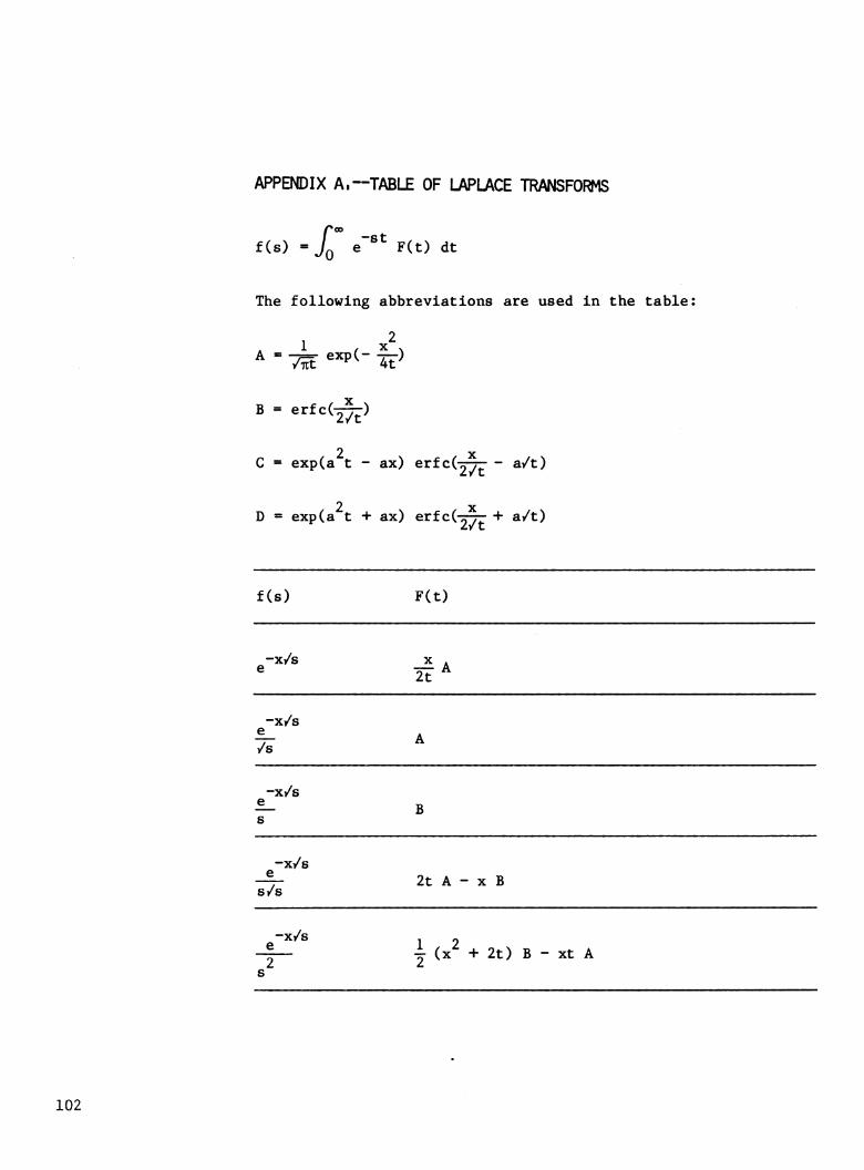
APPENDIX A.—TABLE OF LAPLACE TRANSFORMS
^0 f(s) = L e"^^ F(t) dt
The following abbreviations are used In the table:
A = -^ exp(- 1^)
B = erfcC^^)
2 X C = exp(a t - ax) erf 0(271" "" a/t)
2 X D = exp(a t + ax) erfCC-^TT + a/t)
f(s) F(t)
^-x/s "^ A 2t ^
-x/s e /s A
-x/s e s B
-x/s
s/s 2t A - X B
-x/s , 2 ® (x + 2t) B - xt A 2 2
s
102
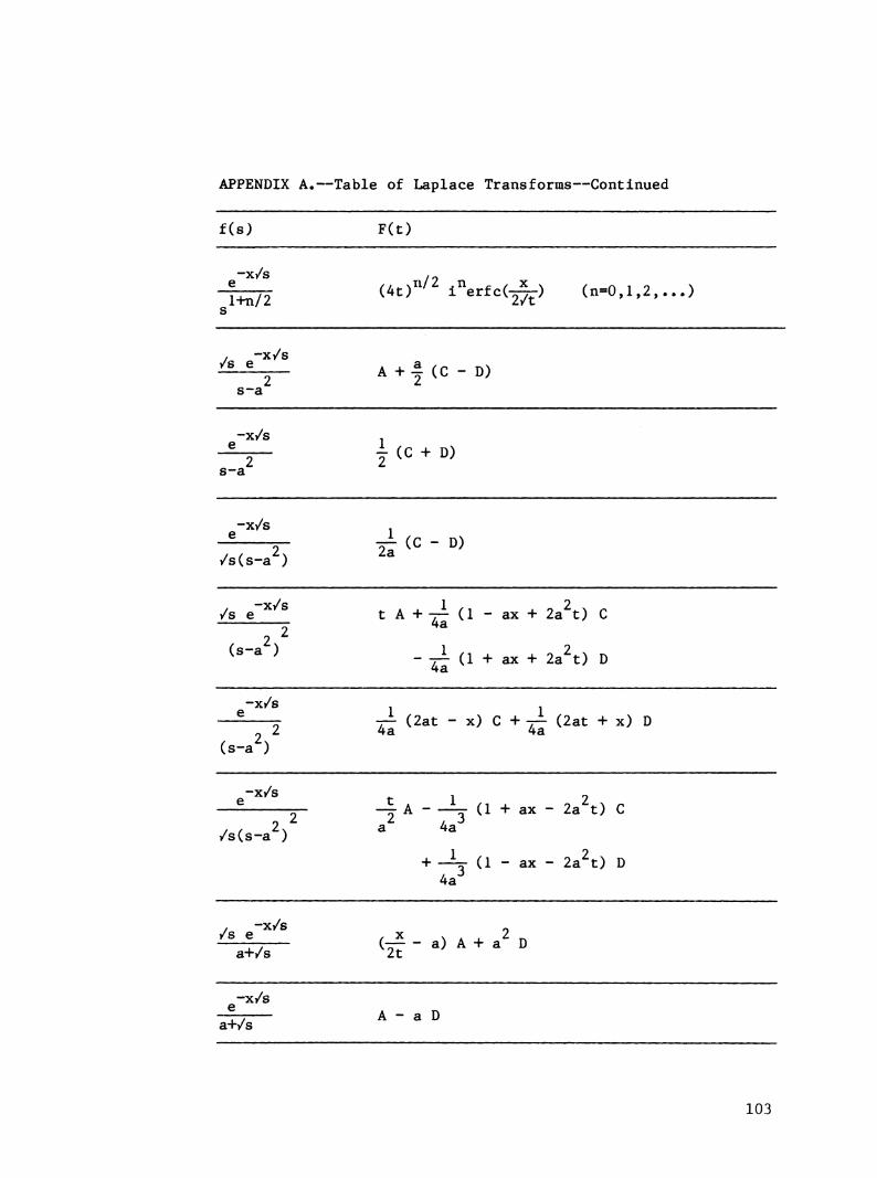
APPENDIX A.—Table of Laplace Transforms—Continued
f(s) F(t)
^ (4t)''^^ i"erfc(^) (n=0,l,2,...) l+n/2 '^' """"'2/t
s
/ -x/s /se . ■ a
2 2 s-a
A +4 (C - D)
e"^»"^ 1 2 2
8-a ^ (C + D)
-x/s , e 1
/ / 2v 2a /s(s-a )
(s-a')
■e (C - D)
/s e""^*^^ t A + 7^ (1 - ax + 2a^t) C
—2 '^
^^"^ ^ - 7^ (1 + ax + 2a^t) D 4a
-x/s . ^ 2 4"^ (2at - x) C + -^ (2at + x) D
-x/s , „ 2~ -^ A - -ij (1 + ax - 2a^t) C
/s(s-a2) ^ "^^
+ -Xr (1 - ax - 2a^t) D 4a-^
/ -x/s „ /se , X \ . . 2
a+/s ^2t
-x/s e
a+/s
(^ - a) A + a D
A - a D
103

APPENDIX A.—Table of Laplace Transforms—Continued
f(s) F(t)
-x/s e /s(a+/s)
-x/s , e 1
s(a+/s) a - (B - D)
^x^s
a a
1 2 12 2 -x/s —7 (14-ax + at+-=rax) B
e J z a
s (a+/s) - -j D - -| (2 + ax) A
a a
8
-x/s , r n-1 "I
y« e~ ® 11 2 '^ -f C + 4- (3 + 2ax + 4a t) D - at A (8-a^)(a+/8) ^ *
-x/s , , „ ® tA+TÍC-7-í^(l + 2ax + 4a t) D
(8-a^)(a+/8) ** **
—x/s ^^ -^ C + -^ (-1 + 2ax + 4a^t) D - -| A /s(s-a )(a+/s) 4a 4a
-x/s ,3 ,3 e 4a 4a
^ C + -^3 - 2ax - 4a^t) D
2 s(s-a )(a+/s)
a a
104
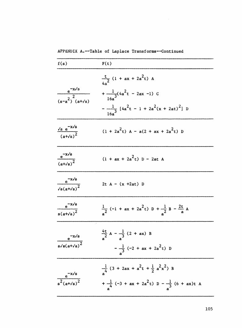
APPENDIX A.—Table of Laplace Transforms—Continued
f(s) F(t)
(s-a ) (a+/s)
(a+/s)^
-^- (1 + ax + 2a^t) A
e"^"^^ , 1 ., 2
l}, . . . 16a^ + —^4a t - 2ax -1) C
16a^ ^ [4a^t - 1 + 2a^(x + 2at)^l D
'^^ ® (1 + 2a^t) A - a(2 + ax + 2a'^t) D
e"^^" „ . . „ 2
(a+/s)^ (1 + ax + 2a t) D - 2at A
-x/s e
/s(a+/s)^ 2t A - (x +2at) D
2 ^ (-1 + ax + 2a^t) D + -| B - ^ A 8(a+/s) a a
-x/s At A _ _1 (2 + ,,) B e a a
«'^«^-•^•^«>' - 4 (-2 + ax + 2a2t) D a
-^ (3 + 2ax + a^t + -| a^x^) B -x/s a e
s^(a+/s)^ + -^ (-3 + ax + 2a^t) D - -j (6 + ax)t A a a
105

106
APPENDIX A.—Table of Laplace Transforms—Continued
f(s) F(t)
, -x/s I- (3 + ax + 2a^t) A + -^^ C /se 2 8a
(s-a2)(a+/s)2 _ _i ^^ ^ g^^ + ^^ ^2^ + 2a2(x + 2at)2] D
^ C - -rî- (1 + ax + 2a^t) A / Q 2 2a -x/s 8a e
2 2 (s-a )(a+/s) + 1 [_i + 2ax + 8a^t + 2a^(x + 2at)^l D
8a^
-x/s -^ (-1 + ax + 2a^t) A + -^ C 2a2 8a3
/s(s-a )(a+/s)
-ir- [1 - 2ax + 2a'^(x + 2at)'^] D 8a-^
16a^ ^ [1 + a(4a^t - l)(x + 2at)
® +4 a^(x + 2at)^] D 2 3 2/, . , x2 -^ (s-a ) (a+/s)
16a^ ^ (1 + ax - 2a^t) C
12a3 ^ [-3 + 4a^t + a^(x + 2at)^] A
-!^^-^ ^ [1 + 2ax + Sa'^t + |- (x + 2at)^] D (a+/s)-^ ^
2 - at(4 + ax + 2a t) A
e"^'^^ t(2 + ax + 2a^t) A
(a+/s)^ - [x + 3at + "I (x + 2at)^] D

APPENDIX A.—Table of Laplace Transforms—Continued
f(8) F(t)
-x/s e
It + I" (x + 2at)^] D - t(x + 2at) A /s(a+/8)^
-x/s e
—^- [-3 + 3ax + 14a\ + 2a^(x + 2at)^] A 12a^
(s-a^)(aVs)^ + -^ [C + (2ax - 1) D] 16a-^
" ifc i^^'^ "^ 2at)(x + 6at) + 2a(x + 2at)^] D
/ -x/s /s e
(a+/s)^
2 t[2 + 2ax + ^ a\ + |- (x + 2at)^] A
- [x + at + a(x + 2at)(x + 3at)
2 „ + ^ (x + 2at)-^l D
-x/s e [t + j (x + 2at)(x + 4at) + f (x + 2at)^] D
- 1 [3x + 10 at + a(x + 2at)^] A
(a+/s)^
-x/s y [4t + (x + 2at)^] A
- [t(x + 2at) + -i (x + 2at)^] D 0
/s(a+/s)^
-x/s 1 r - 1 n 2(a+b) ^ 2(a-b) °
(s-a^)(b+/s) + 2 ^ ^ exp(b^t + bx) erfc(^ + b/t)
a - b
107

APPENDIX B.—SELECTED COMPUTER PROGRAMS
This appendix contains a series of tables listing user-oriented computer programs of several key analytical solutions of the one-dimensional convective-dispersive transport equation. Each program is augmented with sample input data and associated listings of the computer printout. The sample programs con- sidered are those for cases Al (together with A2), A3, B14, and C8. A numerical computer solution (Nl) is also provided. This solution may be used for those cases where no analytical solu- tion is available.
Table 2 (page 111) lists the most significant variables in the computer programs. The names of similar variables in different programs have been kept the same whenever possible. Table 3 lists the sample input data used for the five computer pro- grams. A listing of the function EXF, which is common to all programs except Nl, is given separately in table 4. This function will be discussed below. Listings of the programs themselves, together with the computer output, are given in tables 5 and 6 for case Al, tables 7 and 8 for case A3, tables 9 and 10 for case B14, tables 11 and 12 for case C8, and tables 13 and 14 for case Nl (the numerical solution).
The function EXF(A,B), which appears in all programs except Nl, is listed in table 4. This function defines the product of the exponential function (exp) and the complementary error function (erfc) as follows
EXF(A,B) - exp(A) erfc(B) [Bl]
where
erfc(B) =-^ / " exp(-T^) dx. [B2]
Two different approximations are used for EXF(A,B). For 0 < B < 3 (see also equation [7.1.26] of Abramowitz and Stegun 1970):
EXF(A,B) ^ exp(A - B^)(ajT + a^x^ + a^x^ + a^x^ + a^x^) [B3]
where
'^ ^ 1 + 0.3275911 B f^^
108

aj » .2548296 32 = -.2844967
33 - 1.421414 34 = -1.453152
85 « 1.061405 [B5]
and for B > 3 (see also equation [7.1,14] of Abramowitz and Stegun 1970):
EXF(A,B) ^ j- exp(A - B^)/(B + 0.5/(B + l./(B + [B6]
1.5/(B + 2./(B + 2.5/(B + 1.)))))).
For negative values of B, the following additional relation is used:
EXF(A,B) = 2 exp(A) - EXF(A,-B), [B7]
The function EXF(A,B) can not be used for very small or very large values of its arguments A, B, The function returns zero for the following two conditions:
|A| > 170 |A - B^l > 170 [B8]
B < 0 ^^ B > 0
The computer programs for the analytical solutions are all written in double precision FORTRAN IV; they produce answers that have an accuracy of at least four significant digits. Initially, some problems were encountered with an accurate evaluation of the approximate solutions for the finite systems, especially those that are applicable to flux-type soil surface boundary conditions (cases A4, C8). These approximate solu- tions require the addition and substraction of very large numbers, leading to large roundoff errors and an overall accuracy of at most three significant places when P > 100. The following procedure, first suggested by Brenner {1962)^ was used to derive alternative and more easily evaluated forms of the approximate solutions.
As an example, consider the approximate solution C^¿^ of case A4. This solution can be written in the form
c^4 - c^2 "^ G(x,t) [B9]
where c^ is the analytical solution of case A2 and where G(x,t) is given by
2 ^/2 2
109

exp(vL/D) erfc^^^^"''^ ^i/^1 [BIO] L 2(DRt)^2 J
The approximate solution is used only for relatively large values of the argument in the erfc-function of [BIO]. A suitable asymptotic expansion for erfc is therefore (equation 7.1.23 of Abramowitz and Stegun 1970):
erfc(B) -^^^^^[l -H I ("D" [1 >3... .(2m^l) ] )
Substituting [Bll] into [BIO] and combining appropriate terms allows several of the lead terms in the series to be cancelled. Additional simplification leads to the new form
2 '/2 2 o/ 4.\ /^v tv .vL R ,^- . vtv T
-^1 /'2Dt ™ roT (m-l)vti : (-l)'^^I1.3....(2m-l)] (^> [2L-X-—^—] 1 ;^^SS:i IB12]
■"=' (2L-X + ^)
This series expansion converges rapidly; at most five terms of the series are needed to generate answers that have an accuracy of 4 significant digits. An important advantage of [B12] is that the expression now can be evaluated easily in single precision arithmetic without affecting the four-place accuracy. However, the double precision format of the computer programs has been retained for the present. Wherever necessary, asymptotic expansions similar to [B12] for case A4 were derived also for the other cases involving a finite system; they have been included in the computer solutions.
The numerical solution Nl, listed in table 13, is based on a linear finite element approximation of the spatial derivatives in the transport equation and a third-order finite difference approximation of the time derivative. The theoretical basis of this particular scheme is discussed elsewhere (van Genuchten 1977 , van Genuchten and Gray 1978) and will not be reviewed here. The program assumes that the nodal spacing (DELX) and the time increment (DELT) remain constant.
110

Table 2.—List of the most significant variables in the computer programs
Variable
APRX
BETA
C
C(I)
CO
CA, CB
CI
CONC
Definition
Variable to indicate if the solution for a semi-infinite system can be used to approx- imate the solution for a finite system: APRX = x/L - 0.9 + 8/P. (A3, C8).
Dummy variable for the I-th eigenvalue, G(I). (A3, C8).
Dummy variable for concentration, c.
Nodal values of concentration (Nl).
Constant input concentration, C •
Constants (C^, C^) in several boundary conditions (see table 1). (B14, Nl).
Constant initial concentration, C^*
Concentration, c.
CONS(V,D,R,...) Subroutine to calculate the concentration for a finite profile (A3, C8).
D
DBND
DELT
DELX
DONE
DT
DX
DZERO
Dispersion coefficient.
Constant (a) in several boundary conditions (see table 1). (B14, C8).
Time increment in numerical solution (Nl).
Nodal distance in numerical solution (Nl).
First-order rate coefficient for decay, y. (C8, Nl).
Increment in time for computer printout.
Increment in distance for computer printout.
Zero-order rate coefficient for production, y. (B14, Nl).
Ill
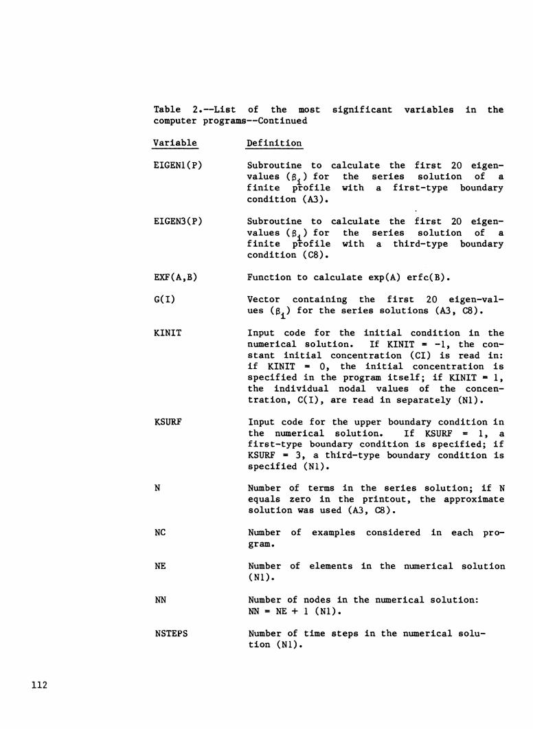
Table 2.—List of the most computer programs—Continued
significant variables in the
Variable Definition
ElGENl(P) Subroutine to calculate the first 20 eigen- values (ß.) for the series solution of a finite profile with a first-type boundary condition (A3).
E1GEN3(P) Subroutine to calculate the first 20 eigen- values ( ß. ) for the series solution of a finite profile with a third-type boundary condition (C8).
EXF(A,B)
G(I)
KINIT
Function to calculate exp(A) erfc(B).
Vector containing the first 20 eigen-val- ues (3 ) for the series solutions (A3, C8).
Input code for the initial condition in the numerical solution. If KINIT = -1, the con- stant initial concentration (CI) is read in: if KINIT = 0, the initial concentration is specified in the program itself; if KINIT = 1, the individual nodal values of the concen- tration, C(I), are read in separately (Nl).
KSURF Input code for the upper boundary condition in the numerical solution. If KSURF = 1, a first-type boundary condition is specified; if KSURF = 3, a third-type boundary condition is specified (Nl).
N Number of terms in the series solution; if N equals zero in the printout, the approximate solution was used (A3, C8).
NC Number of examples considered in each pro- gram.
NE Number of elements in the numerical solution (Nl).
NN Number of nodes in the numerical solution: NN = NE + 1 (NI).
NSTEPS Number of time steps in the numerical solu- tion (Nl).
112
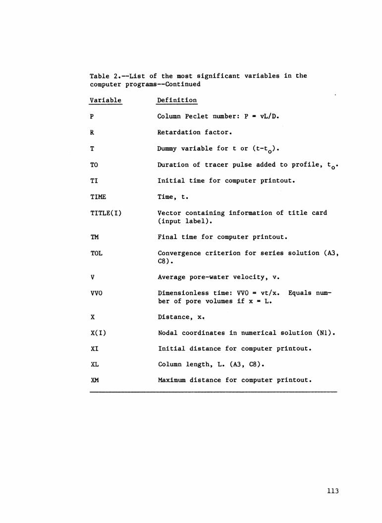
Table 2.- computer
Variable
P
R
T
TO
TI
TIME
TITLE(I)
TM
TOL
V
WO
X
X(I)
XI
XL
XM
—List of the most significant variables in the programs—Continued
Definition
Column Peclet number: P * vL/D.
Retardation factor.
Dummy variable for t or (t-t^).
Duration of tracer pulse added to profile, t^.
Initial time for computer printout.
Time, t.
Vector containing information of title card (input label).
Final time for computer printout.
Convergence criterion for series solution (A3, C8).
Average pore-water velocity, v.
Dimensionless time: WO = vt/x. Equals num- ber of pore volumes if x * L.
Distance, x.
Nodal coordinates in numerical solution (Nl).
Initial distance for computer printout.
Column length, L. (A3, C8).
Maximum distance for computer printout.
113
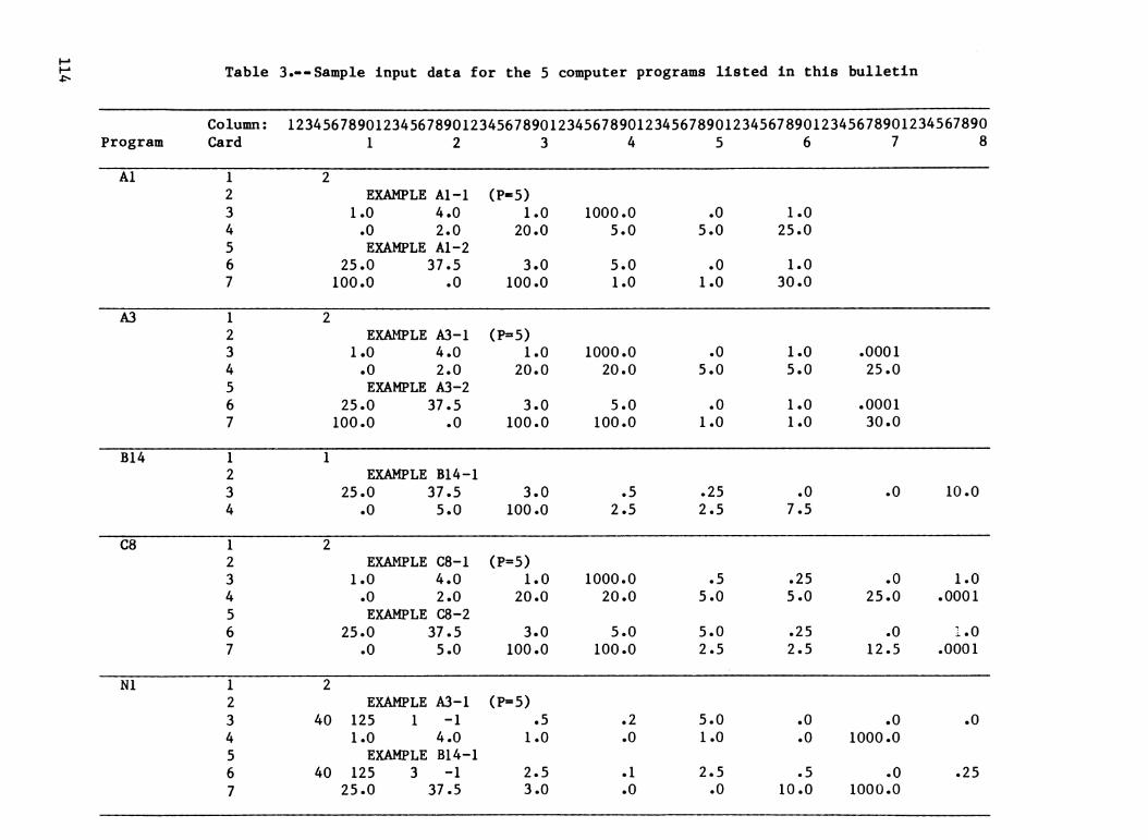
Table 3.--Sample input data for the 5 computer programs listed in this bulletin
Column: 12345678901234567890123456789012345678901234567890123456789012345678901234567890 Program Card 1 2 3 4 5 6 7 8
Al 1 2
2 EXAMPLE Al-1 (P"5)
3 1.0 4.0 1.0 1000.0 .0 1.0 4 .0 2.0 20.0 5.0 5.0 25.0 5 EXAMPLE Al-2 6 25.0 37.5 3.0 5.0 .0 1.0 7 lOO.O .0 100.0 1.0 1.0 30.0
A3 1 2
2 EXAMPLE A3-1 (P=5)
3 1.0 4.0 1.0 1000.0 .0 1.0 .0001 4 .0 2.0 20.0 20.0 5.0 5.0 25.0 5 EXAMPLE A3-2 6 25.0 37.5 3.0 5.0 .0 1.0 .0001 7 lOO.O .0 100.0 100.0 1.0 1.0 30.0
B14 1 2
1 EXAMPLE B14-1
3 25.0 37.5 3.0 .5 .25 .0 .0 10.0 4 .0 5.0 100.0 2.5 2.5 7.5
C8 1 2
2 EXAMPLE C8-1 (P=5)
3 1.0 4.0 1.0 1000.0 .5 .25 .0 1.0 4 .0 2.0 20.0 20.0 5.0 5.0 25.0 .0001 5 EXAMPLE C8-2 6 25.0 37.5 3.0 5.0 5.0 .25 .0 1.0 7 .0 5.0 100.0 100.0 2.5 2.5 12.5 .0001
Nl 1 2
2 EXAMPLE A3-1 (P=5)
3 40 125 1 -1 .5 .2 5.0 .0 .0 .0 4 1.0 4.0 1.0 .0 1.0 .0 1000.0 5 EXAMPLE B14-1 6 40 125 3 -1 2.5 .1 2.5 .5 .0 .25 7 25.0 37.5 3.0 .0 .0 10.0 1000.0

Table 4.—Fortran listing of the function EXF(A,B) = exp(A) erfc(B)
EXF
FUNCTICN EXPÍA,BJ C C PURPOSE: TO CALCULATE EXPÍA) ERFCÍBJ C
IMPLICIT REAL*8 ÍA-H,0-Z) EXF=0.0 IFÍIDABSÍA).GT.170.J.AND.ÍB.LE.0.)) RETURN IF(B.NE.O.O) GO TO 1 EXF=DEXP(A) RETURN
1 C=A-B*B IFi(DABS(C).GT.170.).AND.(B.GT.O.)) RETURN IF(C.LT.-170.) GO TO 4 X=DABSÍB) IFÍX.GT.3.0) GO TO 2 T=l./(!•+.32759I1*X) Y=T*i.2548296-T*(.2844967~T*(1.421414-T*(1.453152-1.061405*T)J)J GO TO 3
2 Y=.5641896/(X+-5/(X+l./<X+1.5/iX+2./(X+2.5/CX+l.J))))) 3 EXF=Y*DEXP(C) 4 IFÍB.LT.O.O) EXF=2.*0EXP{AJ-EXF
RETURN END
115
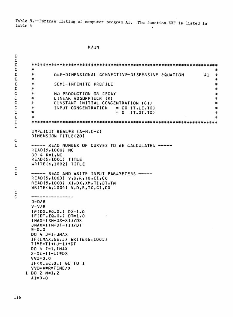
Table 5.—Fortran listing of computer program Al. The function EXF is listed in table 4
MAIN
C c
C * * C * GNE-DIMENSIQNAL CCNVECTIVE-DISPERSlVE EQUATION Al * C * * C * SEMI-INFINITE PROFILE * C * * C * NÜ PRODUCTION OR CECAY ♦ C * LINEAR ADSORPTICN (R) * C * CONSTANT INITIAL CONCENTRATION tCIJ * C * INPUT CGNCENTRATICN = CO (T.LE.TOJ * C * =0 (T.GT.TO) * C * *
C IMPLICIT REAL*8 (A-H,C-Z) DIMENSION TITLE(20)
C C READ NUMBER OF CURVES TO dE CALCULATED
READ(5,1000) NC DO ^ K=1,NC READ(5,I001) TITLE WRITE{6,1002) TITLE
C C READ AND WRITE INPUT PARAMETERS
READ(5,1003) V,D,R,TO,CI,C0 READ(5.1003i XI,DX,XM,TI,DT»TM WRITE(6,1004) V,D,R,TC,CI,CO
C C
D=D/R V=V/R IFiDX.Eû.O.) DX=1.0 IF(DT.EQ.O.) DT=1.0 IMAX=(XM+DX-XIJ/DX JMAX=(TM+DT-TI)/DT E=0.0 DO 4 J=1,JMAX IF(IMAX.GE.J) WRITE(6,1005) TIME=TI+(J-1)*DT DO 4 I=1,IMAX X=XI+(I-1J*DX VVO=0.0 IFiX.Et.O.) GO TO 1 VVO=V*R*TIME/X DO 2 M=l,2 A1=0.0
116

MAIN
A2=0.0 T=TIME+(1-M)*T0 IFÍT.LE.O.) GO TO 2 CM=(X-V*T)/DSQRT(4.*D*T) CP=iX+V*T)/0SQRTÍ4.*D*T) Q=V*X/D A1=0.5*(EXF(E,CMJ+EXF(C,CP)) A2=0.5*EXF(E,CM)+V*DSCRT{.3183099*1/jJ*EXFi-CM*CM,c)-0.5*(l.+w+V*V 1*T/0)*EXF(Q,CP) IF(M.EG.2) GO TO 3 CONC1=CI+(CO-CI)*A1 CONC2=CI+(CO-CI)*A2
2 CONTINUE 3 CONC1=CONC1-CO*A1
C0NC2=C0NC2-C0*A2 4 WRITE(6,1006) X,TIMEtVVC»CCNCl,C0NC2
1000 F0RMAT(I5) 1001 FCRMAT(20A4) 1002 F0RMAT(lHl,10X,82iIH*)/llX ,1H*,80X,iH*/liX,IH*,9X, 'ONE-DIMENSIONAL
1 CQNVECTIVE-DISPERSIVE ECUATION«,25X,lH*/iiX,1H*»äOX,1H*/11X,1H*, 29X,«SEMI-INFINITE PROF ILE• ,50X,1H*/1IX,IH*,9X,«NO PRODUCTION AND D 3ECAY',48X,1H*/11X,1H*,9X,•LINEAR ADSORPTION ÍR)•,50X,1H*/11X,IH*,9 4X,«CONSTANT INITIAL CONCENTRATION (CI)•,36X,1H*/11X,IH*,9X,« INPUT 5C0NCENTRATI0N = CO (T .LE .TO « ,37X, lH*/liX,lH*,29X, •= 0 (T.GT.TOJ« 6,37X,lH*/llX,lH*,80X,lH*/llX,lH*,20A4,lH*/ilX,lH*,80X,lH*/llX,82(l 7H*))
1003 F0PMATÍ8F10.0) 1004 FORMAT(//ilX,«INPUT PARAMETERS«/IIX,16(lH=i//IIX, « V =«,F12.4,15X,•
ID =« ,F12.4/ilX,«R =«,F12.4,15X,«T0 =',F11.4/11X,«CJ =«,Fii.4,15X,« 2C0 =«,F11.4}
1005 FORMAT(///IIX, «DISTANCE«,11X,«TIME«t7X,«PuKE VOLUME«,12X,«CONCENTR 1ATI0N«/14X,«(X)«,i3X,«ÍTJ« ,11X,«(VVOJ «,ÓX,« FIRST-TYPE BC«,4X,«THIR 2D-TYPE BC«)
1006 F0RMAT(4X,3(5X,F10.4),3X,F12.4,5X,F12.4J STOP END
117

Table 6.—Sample output from computer program Al
4c3«c4c4c3ee:(c3«e«:(e:«e«4e4c4c4(3ee4(:Oc:tc4c;tc30e;íe:9e:O(:ec:OE:ec4c:«c3O(*«4t4(4[««««««^^**1t4c4e^
* ONÊ-OIMENSIONAL CONVECTIVE-CISPERSIVÊ EQUATION
SEMI-INFINITE PROFILE NO PRODUCTION AND DECAY LINEAR ADSORPTION ÍR) CONSTANT INITIAL CONCENTRATION (CD INPUT CONCENTRATION = CO (T.LE.TO)
= 0 (T.GT.TO)
EXAMPLE Al-1 (P=5)
:«c4e:9e:ec3tc:«c3gc4c:ec«30c:^:ee:ec:ie:Qc:^:eciOc:ee4c:9e3ec:jc4c«4e3gc*:íeaS.«:e(3Sc:4e^4(4í«:ecXe3fic:ic«
INPUT PARAMETERS
V = 1.0000 R = 1.0000 CI = 0.0
D = 4.0000 TO = 1000.0000 CO = 1.0000
DISTANCE (X)
0.0 2.0000 4.0000 6.0000 8.0000 10.0000 12.0000 14.0000 16.0000 18.0000 20.0000
TIME (T)
5.0000 5.0000 5.0000 5.0000 5.0000 5.0000 5.0000 5.0000 5.0000 5.0000 5.0000
PORE VOLUME (WO)
0.0 2.5000 1.250C C.8333 0.^250 0.5000 0.4167 0.3571 0.3125 C.2778 G.25C0
CONCENTRATION FIRST-TYPE BC THIRD-TYPE BC
1.0000 0.9036 0.7731 0.6209 0.4648 0.3224 0.20ö4 0.1215 0.0635 0.0324 0.014Ó
0.7640 0.6376 0.5023 0^3712 0.2559 0.1638 0.0970 0.0530 0.0266 0.0123 0.0052
DISTANCE (X)
0.0 2.0000 4.0000 6.0000 8.0000 10.0000 12.0000 14.0000 16.0000 18.0000 20.0000
TIME (TJ
10.0000 10.0000 IC.OOOO 10.0000 10.0000 10.0000 10.0000 10.0000 10.0000 lO.QOOO 10.0000
PORE VCLUME (WO)
0.0 5.000C 2.5000 1.6667 1.2500 1.0000 C.8333 C.7143 0.625C C.5556 C.500C
CONCENTRATION FIRST-TYPE BC THIRD-TYPE BC
1.0000 0.9626 0.9086 0.8377 0.7517 0.6544 0.5512 0.44öl 0.350Ö 0.2641 0.1909
0.8845 0.8198 0.7424 0.6548 0.5610 0.4657 0.3738 0.2895 0.2161 0.1551 0.1070
DISTANCE (X)
0.0 2.0000
TIME (Ti
15.0000 15.0000
PORE VOLUME (VVC) CO 7.50C0
CONCENTRATION FIRST-TYPE BC THIRD-TYPE BC
1.0000 0.9365 0.9818 0.9003
118

4.0000 6.0000 8.0000 10.0000 12.0000 14.0000 16.0000 18.0000 20.0000
15.0000 15.0000 15.0000 15.0000 15.0000 15.0000 15.0C00 15.0000 15.0000
3.75CC 2.500C 1.875C 1.50C0 1.25CC 1.C714 0.9375 C.8333 C.750C
0.9549 0.9181 0.8707 0.8129 0.7456 0.6707 0.5907 0.5087 0.4278
0.8549 0.8004 0.7375 0.6677 0.5931 0.5161 0.4394 0.3656 0.2969
DISTANCE (X)
0.0 2.0000 4.0000 6.0000 8.0000 10.0000 12.0000 14.0000 16.0000 18.0000 20.0000
TIME (T)
20.0000 20.0000 20.0000 20.0000 20.0000 2C.0000 20.0000 20.0000 20.0000 2C.0000 20.0000
PORE VOLUME (VVC) CO
IC.OOOO 5.0OC0 3.2333 2.5000 2.C0GC 1.66é7 1.^286 1.2500 1.1111 l.OOCO
CONCENTRATION FIRST-TYPE BC THIRD-TYPE BC
1.0000 0.9902 0.9756 0.9551 0.9278 0.8933 0.8511 0.8014 0.7449 0.6827 0.6162
0.9630 0.9416 0.9142 0.8801 0.8392 0.7916 0.7379 0.6788 0.6157 0.5501 0.4837
DISTANCE (X)
0.0 2.0000 4.0000 6.0000 8.0000 10.0000 12.0000 14.0000 16.0000 18.0000 20.0000
TIME ÍT)
25.0000 25.0000 25.0000 25.0C00 25.0000 25.0000 25.0000 25.0000 25.0000 25.0000 25.0000
PORE VOLUME (VVC) CO
12.5000 6.2500 4.1667 3.125C 2.50CC 2.0833 1.7657 1.5625 1.3889 1.2500
CONCENTRATION FIRST-TYPtf
1.0000 0.9944 0.9860 0.9740 0.9578 0.9368 0.9103 0.8780 0.8399 0.7960 0.7467
BC THIRD-TYPE BC 0.9776 0.9646 0.9476 0.9261 0.8995 0.8677 0.8304 0.7879 0.7404 0.6886 0.6334
119

:¡^i^:^^:^:¡^:tliiíí:í^:(,:i^i(lí7^:tí^:^:t¡t:iii:i^iti:tíi^:í^ilt:fli:ti:^i(li:^
* *
*
*
ONE-DIMENSIONAL CONVECTIVE-CISPERSIVE EQUATION
SEMI-INFINITE PROFILE NO PRODUCTION AND DECAY LINEAR ADSORPTION ÍR) CONSTANT INITIAL CONCENTRATION (CD INPUT CONCENTRATION = CO (T.LE.TO)
= 0 (T.GT.TO)
EXAMPLE Al-2
*
*
30c
aie
4c :0c 4c ^ 4c :ec 4e :«( :Ac :9c :^ :«( ^Qc :^ :«e :^ 4c :«c 39e :Qe :«( :9c :9e :Cc :ec :0c # ♦ 34c 34c 41 :(c 4t :(( 30c :«c 4c :(c :«c :te :«c JÍC :^
INrUT PARAMETERS
V = R = CI =
25.0000 3.0000 0.0
D = TO =
37.5000 5.0000
CO = 1.0000
DISTANCE TIME PORE VCLUME CONCENTRATION (X) ÍT) (WO) FIRST-TYPE BC THIRD-TYPE
100.0000 1.0000 C.2500 0.0000 0.0000 100.0000 2.0000 C.5000 0.0000 0.0000 100.0000 2.0000 0.7500 0.0000 0.0000 100.0000 4,0000 l.COCO 0.0000 0.0000 100.0000 5.0000 1.250C 0.0000 0.0000 100.0000 6.0000 1.5000 0.0000 0.0000 100.0000 7.0000 1.7500 0.0010 0.0008 100.0000 8.0000 2.0000 0.0113 0.0088 100.0000 9.0000 2.2500 0.0563 0.0465 100.0000 10.0000 2.500C 0.1655 0.1439 100.0000 11.0000 2.7500 0.337b 0.3059 100.0000 12.0000 3.0000 0.5332 0.4987 100.0000 13.0000 3.2500 0.6975 0.6700 100.0000 14.0000 3.5CCC 0.7b02 0.7ÖÖ4 100.0000 15.0000 3.7500 0.7509 0.7592 100.0000 16.0000 4.0CC0 0.6228 O.0474 100.0000 17.0000 4.25C0 0.4485 0.4795 100.0000 18.0000 4.50C0 0.2840 0.3124 100.0000 19.0000 4.7500 0.1607 0.1816 100.0000 20.0000 5.00C0 0.0825 0.0956 100.0000 21.0000 5.25CC 0.0389 0.0462 100.0000 22.0000 5.50C0 0.0171 0.0208 100.0000 23.0000 5.7500 0.0071 0.0088 100.0000 24.0000 6.0000 0.0028 0.0035 100.0000 25.0000 6.2500 0.0010 0.0013 100.0000 26.0000 6.5000 0.0004 0.0003 100.0000 27.0000 6.7500 0.0001 0.0002 100.0000 28.0000 7.0000 0.0000 0.0001 100.0000 29.0000 7.2500 0.0000 0.0000 100.0000 30.0000 7.5000 0.0000 0.0000
BC
120
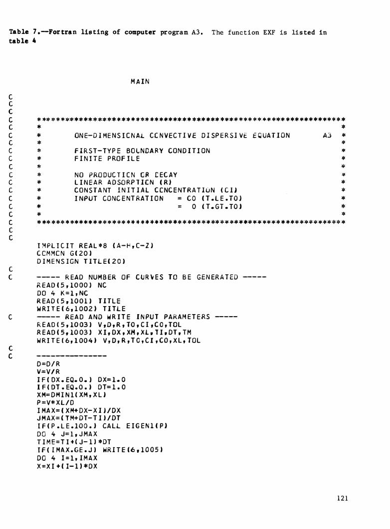
Table 7.—Fortran listing of computer program A3. The function EXF is listed in table 4
MAIN
C C C
C * * C * ONE-DIMENSICNAl CCNVECTIVE DISPERSIVE ÉQUATION AJ » C * * C * FIRST-TYPE BOLNDARY CONDITION * C * FINITE PROFILE * C * * C * NO PRODUCTICN C« CECAY » C * LINEAR ADSORPTICN (R) * C * CONSTANT INITIAL CCNCENTRATIÙN (CIJ * C * INPUT CONCENTRATION = CD (T.LE.TO) * C * =0 ÍT.GT.TO) * C * *
C C
IMPLICIT REAL*8 (A-H,C-2} CGMMCN G(20) DIMENSION TITLEÍ20)
C C READ NUMBER OF CURVES TO BE GENERATED
REA0Í5,1000) NC DO 4 K=1,NC READ(5,1001) TITLE WRITE(6,1002) TITLE
C READ AND WRITE INPUT PARAMETERS READ(5,1003) V,D,RtTO,CItC0,TOL READÍ5,1003) XI,DX,XM,XL,TI.DT,TM WRITE(6,1004) V,D,RfTC,CI,CO,XL,TOL
C
D=D/R V=V/R IF(OX.£Q.O.) DX=1.0 IF(DT.EQ.O.) DT=1.0 XM=DMIN1(XM,XL) P=V*XL/D IMAX=(XM+DX-XI)/DX JMAX=ÍTM+DT-TI)/DT IFÍP.LE.100.) CALL EIGENKP) DO 4 J=1,JMAX TIME=TI+(J-1)*DT IF(IMAX.GE.J) WRITE(6,1005) DO 4 I=1,IMAX X=XI+(I-1)*DX
121

c c
MÍIN
vva=o.o IFÍX.EQ.O.) GO TO 1 VVO=V*R*TIME/X
1 DO 2 M=l,2 C=0.0 T=TIME+(1-M)*T0 IF(T.LE.C.) GO TO 2 CALL CCNS(C,V,D,X,T,XL,TOL,NJ IF(M.EQ.2) GO TO 3 CCNC=CI+iCO-CIi*C
2 CONTINUE 3 CCNC=CCNC-CO*C 4 WRITE(6,1006) X, TIME, VVCCCNC, N
1000 FORMATdS) 1001 FORMAT(20A4} 1002 F0RMAT(1H1,10X,82(IH*)/IIX ,1H*,80X ,1H*/11X,IH*,9X,'ONE-DIMENSIONAL
1 CCNVECTIVE-DISPERSIVE ECUATIüN',25X,1H*/11X,1H*,80X,lH*/llX,lH*t9 2X,«FIRST-TYPE BOUNDARY CCNDITION•,42X,1H*/1IX,1H*,9X,'FINITE PROFI 3LE«,57X,lH*/llX,lH*,8CX,lh*/llX,lH*,9X,«Nü PRODUCTION Cft DECAY«,49 4X,1H*/11X,1H*,9X,«LINEAR ACSORPTION (RÍ«,50X,1H*/11X,IH*,9X,«CONST 5ANT INITIAL CONCENTRATICN (CI)•,36X,1H*/11X,1H*,9X,«INPJT CCNCÊNTR 6ATI0N = CO (T.LE.TO)« ,37X,1H*/11X,1H*,29X,«= 0 ÍT.GT.TOJ•,37X,1H* 7/llX,lH*,80X,lH*/llX,lH*,20A4,lH*/llX,lH*,80X,iH*/liX,d2(lH*iJ
1003 FORMAT(8F10.0) 1004 F0RMAT(//11X,«INPUT PARAMETERS'/IIX,16Í1H=J//IIX,•V =« ,F12.4,15X,•
ID =«,F12.4/11X,«R =«,F12.4,15X,«T0 =«,F11.4/11X,«CI =•,F11.4,15X,• 2C0 =«,F11.4/11X,«XL =«,F11.4,15X,«T0L =«,F10.6i
1005 FORMAT(///IIX , «DISTANCE«,IIX,«TIME «,7X,•POKE VOLUME«,6X,«CÜNCENTRA IT ION«.SX,«NUMBER«/14X,«(X)«,13X, «(TJ•,11X,«(VVOi «,14X,•<C)«,7X,«OF 2 TERMS«)
1006 F0RMAT(4X,3{5X,F10.4),8X,F10.4,7X,14) STOP END
122

EIGENl
SUBROUTINE EIGENKP) C C PURPOSE: TO CALCULATE THE EIGENVALUES C
IMPLICIT REAL*8 CA-H,0-Z) COMMON G(20) BETA=0.1 DC 4 1=1,20 J=0
1 J=J+1 IF(J.GT.15) GO TO 3 DELTA=-0.2*(-0.5)**J
2 BET2=BETA BETA=BETA+DELTA A=BET2*0C0S(BET2)+0.5*P*DSIN(BET2) B=BETA*DC0S(BETA)+0.5*P*0SINCBETA) IF(A*B) 1,3,2
3 G(I)=(BET2*B-BETA*AJ/(E-A) 4 BETA=BETA+0.2
WRITE(6,1000) (G(I),I=l,20i 1000 F0RMAT(//11X,«CALCULATED EIGENVALUESVliX,22i1H=J/(8X,5F12.6/JJ
RETURN END
123

CCNS
SUBROUTINE CONSÍC,V,D,X,T,XL,TOL,I) C C PURPOSE: TO CALCULATE CONCENTRATION C C
IMPLICIT REAL*8 (A-H,C-Z) CCMMCN G(20) 1=0 P=V*XL/D Q=V*X/D APRX=X/XL-0.9+8./P IFÍAPRX.LT.O.) GO TO 4 IF(<P.GT.100.).OR.((P-40.*V*T/XL).GT.5.JJ GO TO 4 EX=0.5*Q-0.25*V*V*T/0
C C SERIES SOLUTION
SUM=0.0 IFÍX.EÜ.O.) GO TO 3 DO 2 J=l,10 DSUM=0.0 DO 1 K=l,2 I=2*J+K-2 A=G(I)*DSIN(G(I)*X/XL) IF(DABS(A).LT.l.D-10) A=0.0 EXP=EX-(G(n/XL)**2*D«T IF<DABS(EXP).GT.160.J EXP=-160.
1 DSUM=DSJM+DtXP(£XP)«A/(G{I)**2+0.25*P*P+Û.5*P> SUM=SUM+DSUM 1F{DABS(DSUM/SÜM).LT.TCL) GO TO 3
2 CONTINUE GO TO 4
3 C=1.-2.«SÜM RETURN
C C APPROXIMATE SCLLTICN
4 S=DSQRT(4.*0*T) E=0.0 C=0.5*(EXFÍE,(X-V#T)/S)+EXF(Q,(X+V*T)/SJJ IFÍAPRX.LT.O.) RETURN A=2.*D*T/Í2.*XL-X+V*TJ**2 B=2.*V#T/(2.*XL-XJ C=C+(2.*XL-X)«'A*EXFÍP-0.5/A,E}*(l.-A*((l.-£J-J.*A*((l.-2.*Bj-5.*A* lí(l.-3.*BJ-7.*A*(l.-4.*B))J))/0SQRTÍ3.14i593*u*T) RETURN END
124

Table 8.—Sample output from computer program A3
]Oc:Ct«3ec4e«3t(3|c4c4c:Cc#3|(4t3|c:tc«:^#4c3te:(e^:Cc:tc3Cc4c:OcXc3íc4c3Í(4(«4c:0(3Oc:ec3Oe4c:íe:íc^aAe:^
*
ONE-DIMENSIONAL CONVECTIVE-CISPERSIV£ EQUATION
FIRST-TYPE BOUNCAKY CCNDITICN FINITE PROFILE
NO PRCÛUCTION OR DECAY LINEAR ADSORPTION (R) CONSTANT INITIAL CONCENTRATION (CD INPUT CONCENTRATION = CO (T.LE.TOi
= 0 (T.6T.T0)
EXAMPLE A3-1 (P=5)
i^i^^:^iií^:^i^i^:^i^t^^:^^:iii^^i^ií!i:t!:ilti!::¡^:¡(lt^i(lití^:¡(lt^:flíi(li^^
INPUT PARAMETERS
V = 1.0000 R = 1.0000 CI = 0.0 XL = 20.0000
D = 4.0000 TO = 1000.0000 CO = 1.0000 TOL = 0.000100
CALCULATED EIGENVALUES
2.380644 5.163306 8.151564 11.214906 14.310123
17.421289 20.541462 23.667186 26.796564 29.928469
33.062194 36.197272 39.333382 42.470298 45.607854
48.745928 51.884426 55.023276 58.162421 61.301816
DISTANCE TIME PORE VCLUME CONCENTRATION NUMBER (X) (T) (WO) (C) OF TERMS
0.0 5.0000 CO 1.0000 0 2.0000 5.0000 2.500C 0.9036 6 4.0000 5.0000 1.2500 0.7731 6 6.0000 5.0000 C.8333 0.6209 6 8.0000 5.0000 C.625C 0.4648 6
10.0000 5.0000 C.50C0 0.3ZZ5 6 12.0000 5.0000 0.4167 0.2064 6 14.0000 5.0000 C.3571 0.1216 6 16.0000 5.0000 C.3125 0.0661 6 18.0000 5.0000 C.2778 0.0348 6 20.0000 5.3000 C.250Û 0.0240 6
DISTANCE TIME PCBE VOLUME CONCENTRATION NUMBER (X) (T) (WO) (C) OF TERMS
0.0 10.0000 CO 1.0000 0 2.0000 10.0000 5.COCO 0.9626 6 4.0000 10.0000 2.50CC 0.9086 6
125

6.0000 10.0000 1.6667 0.8378 6 8.0000 10.0000 1.250C 0.7520 6
10.0000 10.0000 l.OCOC 0.6553 6 12.0000 IC.OOOO C.8323 0.5536 6 14.0000 10.0000 C.7143 0.4544 6 16.0000 10.0000 C.6250 0-3666 6 18.0000 10.0000 0.5556 0.3013 6 20.0000 10.0000 C.5ÛC0 0.2747 6
DISTANCE TIME POPE VCLÜME CONCENTRATION NUMBER (X) (T) (WO) ÍC) OF TERMS
0.0 15.0000 CO 1-0000 0 2.0000 15.0000 7.500C 0.*í819 6 4.0000 15.0000 3.7500 0.9553 6 6.0000 15.0000 2.50C0 0.9189 4 8.0000 15.0000 1.875C 0.6726 4
10.0000 15.0000 1.5000 0.8170 4 12.0000 15.0000 1.2500 0.7544 4 14.0000 15.0000 1.071^ 0.6889 4 16.0000 15.0000 C.9375 0.6271 4 18.0000 15.0000 0.8333 Û.5788 4 20.0000 15.0000 C.7500 0.5586 6
DISTANCE TIME PORE VOLUME CONCENTRATION NUMBER (X) (T) (VVC) (CJ OF TERMS
0.0 20.0000 CO 1-0000 0 2.0000 20.0000 IC.CCCO 0.9905 4 4.0000 20.0000 5.00CO 0-9764 4 6.0000 2C.0000 3.3333 0.9569 4 8.0000 20.0000 2.5000 0.9316 4
10.0000 20.0000 2.0000 0.9005 4 12.0000 20.0000 1.6667 0.8648 4 14.0000 20.0000 1.4286 0.8266 4 16.0000 20.0000 1.25C0 0.7899 4 18.0000 20.0000 1.1111 0.7608 4 20.0000 20.0000 1.0000 0.7485 4
DISTANCE TIME PORE VCLUME CONCENTRATION NUMBER (X) (T) (VVC) (C) OF TERMS
0.0 25.0000 CO 1.0000 0 2.0000 25.0000 12.50CC 0.9949 4 4.0000 25.0000 6.2500 0.9872 4 6.0000 25.0000 ^.1667 0.9766 4 8.0000 25i0000 2-1250 0.9626 4
10.0000 25.0000 2.50CC 0.94i>5 4 12.0000 25.0000 2.0823 0.9255 4 14.0000 25.0000 1.7857 0.9041 4 16.0000 25.0000 1.5625 0.8833 4 18.0000 25.0000 1.3889 0.8668 4 20.0000 25.0000 1.25C0 0.8598 4
126

:t¡i:^:^:^:¡^:¡^^:^^^:flíiíiíi::^i^ii¡ii^it^iílí;^i(lt:¡ií^^^i^:^:¡íli:i^^^:(li^
*
*
*
*
ONE-DIMENSIONAL CONVECT IVE-CISPERSIVh EgüATIÜN
FIRST-TYPE BOUNDARY CCNDITICN FINITE PROFILE
NO PRODUCTION Oi< DECAy LINEAR ADSORPTION (R) CONSTANT INITIAL CONCENTRATION (CD INPUT CONCENTRATION = CO (T.LE.TOi
= 0 (T.GT.TO)
EXAMPLE A3-2 *
«*#:íc««***««*«*««:ícXc *«*********♦*♦***♦♦♦♦***♦ Jit**«**********:ec«**«**^*^
INPUT PARAMETERS
V = 25.3C00 R = 3.0000 CI = 0.0 XL = 100.0000
D = 37.5000 TO = 5.0000 CO = 1.0000 TOL = C.000100
CALCULATED EIGENVALUES
3.050337 6.102126 9.15669C 12.215114 15.278191
18.346412 21.419993 24.49893C 27.583053 30.672083
33.765670 36.863467 39.965076 -^3.070143 46.178327
49.289314 52.402819 55.518585 56.636381 61.75o003
DISTANCE TIME PORE VOLUME CONCENTRATION NUMBER (XJ (T) LVVCJ ÍC) OF TERMS
100.0000 1.0000 C.250O 0.0000 0 100.0000 2.0000 C.5000 0.0000 0 100.0000 3.0000 C.750C 0.0000 0 100.0000 4.0000 l.OOCO 0.0000 0 100.0000 5.0CO0 1.2500 0.0000 0 100.0000 6.0000 1.500C 0.0000 0 100.0000 7.0000 1.7500 0.0013 0 100.0000 8.0000 2.COO0 0.0138 0 100.0000 9.0000 2.25CC 0.0660 0 100.0000 IC.OOOO 2.50C0 0.1872 0 100.0000 11.0000 2.750C 0.3697 0 100.0000 12.0000 3.0000 0.5677 0 100.0000 13.0000 3.2500 0.7250 0 100.0000 14.0000 3.5000 0.7920 0 100.0000 15.0000 3.7500 0.7427 0 100.0000 16.0000 ^.OOCO 0.5983 0 100.0000 17.0000 ^.2500 0.4174 0 100.0000 18.0000 4.5000 0.2557 0 100.0000 19.0000 4.7500 0.1399 0
127

lOO.COOü 20.0000 5.00CC 100.0000 21.0000 5.25C0 100.0000 22.0000 5.5CCC lOO.OOCO 23.0000 5.75CC lOO.COOO 2A.0000 é.CCCC lOC.OCOO 25.0000 6.250C 100.0000 26.0000 é.50CC 100.0000 27.0000 6.75C0 100.0000 28.0000 7.COCO lOO.tOOO 29.0000 7.2500 100.0000 30.0000 7.5CC0
0.0694 0 0.0317 0 0.0135 0 0.0054 0 0.0020 12 0.0007 10 0.0003 10 0.0001 10 0.0000 10 0.0000 10 0.0000 10
128

Table 9.—Fortran listing of computer program B14. The function EXF is listed in table 4
MÍIN
C C
c * * C * ONt-DIMENSIONAL CCNVECTIVE-DISPERSIVE EQUATION 614 * C * * C * THIRD-TYPE BOUNCARV CONDITION * C * SEHI-INFINITE FRGFILE * C * ♦ C * ZERÜ-CROER PRCDLCTIÜN (DZERO) * C * LINEAR ADSORPTICN (RJ ♦ C * CONSTANT INITIAL CCNCENTRATION (CD ♦ C * INPUT CONCENTRATICN = CA+CB*EXPi-OBND*T) * C * *
c IMPLICIT REAL*8 ÍA-H,C-ZJ DIMENSION TITLE(20)
C C READ NUMBER OF CURVES TO BE CALCULATED
READ(5,1000) NC DO 4 K=1,NC REA0(5,1001) TITLE WPITE(6,1002) TITLE
C C READ AND WRITE INPUT PARAMETERS
REA0(S),1003) V,D,R,DZ£f<D,CeNDfCI,CA,CB REA0(3,1003) XI,DX,XM,II,CT,TM WRITE{6,1004) V,D,R,DZERütCBND,CI,CA,CB
C C
D = D/R V=V/R DZERO=CZERC/R S=v**2-4.*D3ND*D IF(S.LE.O.) GO TO 5 Y=DSQRT(S) IFiOX.EQ.G.J DX=1.0 IFÍDT.EQ.G.) 0T=1.0 IMAX=(XM+DX-XI)/DX JMAX=(TM+DT-T1)/DT DO 4 J=1,JMAX T=TI+(J-1)*DT IFdMAX.GE.J) WRITE(6,1005J DO 4 I=1,IMAX X=XI+(I-1)*DX VVO=0.0 IF(X.EQ.O.) GO TO 1
129

c c
MAIN
VVO=V*R*T/X 1 P=V*X/D
S=DSQRT(4.*D*T) A1=X-V*T A2=X+V*T AM=0.5*EXF(0.D0,A1/SJ AP=0.5*EXF(P,A2/S) AZ=DSQRT(.3183099*T/D)*EXF(-(A1/S)**2,0.D0J BM=(X-Y*T)/S BP=(X+Y*T)/S CM=0.5*(V-Y)*X/D CP=0.5*(V+Y)*X/D A=AM+V*AZ-(1.+P+V*V*T/D)*AP B=DEXPl-DBND*T)*(V/(V+Y)*EXF(CM,BM)+V/(V-YJ*EXF(CP,BPJ)-V*V*AP/iOB
1ND*D) C0NC=CI+(CA-Cn*A+CB*B+CZ£R0*ÍT+(Al+D/V)*AM/V-.5*ÍA2+2.*D/V)*AZ+(T
l-0/V«*2+.5*A2**2/D)*APJ 4 WRITE(6,1006) X,T,VVC,CCNC
GO TO 6 5 KRITEÍ6,1007) 6 CONTINUE
1000 FORMATdS) 1001 FCRMATÍ20A4) 1002 FCRMAT(1H1,10X,82(1H*)/11X,1H*,80X,1H*/11X,1H*,9X,'ONE-DIMENSIONAL
i CONVECTIVE-OISPERSIVE EGUATION« f25X,1H*/11X,1H*,b0X,1H*,/11X ,lri*# 29X,'THIRD-TYPE BOUNDARY CCNDITION»,42X,lH*/ilX,lH*f9X,«SEMI-INFINI 3TE PROFILE«,50X,1H*/1IX,IH*,80X,1H*/11X,1H*,9X,«LINEAR ADSORPTION 4(R)' ,50X,lH«/llX,lH*f9X,«ZERO-ORDER PRODUCTION (DZEROJ «,42X,1H*/11 5X,1H*,9X,'CONSTANT INITIAL CONCENTRATION (CI)«,36X,1H*/11X,1H*,9X, 6'INPUT CONCENTRATION = CA+CB*EXP(-DBND*T)«,31X,lH*/liX,lH*,80X,lH* 7/llX,lri*,20A4,lH*/llX,lH*,80X,lH*/llX,82(lH*))
1003 FORMATOFIO.O) 1004 F0RMAT(//11X,«INPUT PARAMETERS«/IIX,16ÍiH=J//IIX,«V =«,F12.4,15X,•
ID =•,F12.4/11X,«R =«,F12.4,15X,'DZER0 =« ,F6.4/1IXt«OBND =',F9.4,i5 2X,«CI =',F11.4/11X,«CA =• ,Fil.4,15X,«CB =«,Fil.4)
1005 FORMAT(////IIX,«DISTANCE«,11X,«TIME«,7X,«PORE VOLUME«,6X,«CONCENTR 1ATI0N«/14X,«(X)« ,13X, «(T)« ,11X , « Í WO) « ,14X, « (C J «/)
1006 F0RMAT(4X,3(5X,F10.4J ,8XfF10.4} 1007 F0RMAT(///5X/6(1H*),« CBND IS TOO LARGE, THIS CASE NOT EXECUTED «,
16(1H*)) STOP END
130

Table 10,—Sample output from computer program B14
*
*
ONE-DIMENSIO.MAL CÛNVECT I VE-CISPERSl VE EQUATION
THIRD-TYPE BOUNDARY CCNOITICN SEMI-INFINITE PROFILE
LINEAR ADSORPTICN (R) ZERO-ORDER PRODUCTION (DZERC) CONSTANT INITIAL CONCENTRATION ÍCIJ INPUT CONCENTRATION = CA+CB*EXP(-DBNO*T)
EXAMPLE B14-Í
*
*
* 3ÍC
««**«;íc**:ít«««:íc*:{c*:íc*«:íc:ic:íc3{í:{c«:íc**4t******««****««*****aEc:ít**«*:je*:íc4c
INPUT PARAMETERS
V = 25.C000 R = 3.0000 OBND = 0.2500 CA = 0.0
D = 37.5000 CZERO = = 0.5000 CI = 0.0 Cß = 10.0000
DISTANCE TIME PORE VOLUME CONCENTRATION (X) (T) (WO) (C)
0.0 2.5000 CO 5.6301 5.0000 2.5000 12.5000 6.5099
10.0000 2.5000 6.2500 6.9976 15.0000 2.5000 4.1667 6.5451 20.0000 2.5000 2.1250 4.9945 25.0000 2.5000 2.500C 3.0083 30.0000 2.5000 2.0823 1.4860 35.0000 2.5000 1.7657 0.7302 40.0000 2.5000 1.5625 0.4809 45.0000 2.5000 1.3889 0.4258 50.0000 2.5003 1.250C 0.4176 55.0000 2.5000 1.13^4 0.4167 6U.0000 2.5000 1.0417 0.4167 65.0000 2.5000 C.S615 0.4167 7Ü.0000 2.5000 C.8929 0.4167 75.0000 2.5000 C.8333 0.4167 80.0000 2.5000 C.7812 0.4167 85.0000 2.5000 0.7353 0.4167 90.0000 2.5000 C.6944 0.4167 95.0000 2.5000 0.6579 0.4167 100.0000 2.5000 0.6250 0.4167
DISTANCE (X)
TIME (T)
PORE VOLUME (VVC)
COMCENTKATIüN (Ci
0.0 5.0000
5.0000 5.0000
0.0 25.00C0
3.036Ö 3.6467
131

10.0000 5-0000 12.5000 4.3309 15.0000 5.0000 8.3323 5.0686 20.0000 5.0000 6.2500 5.7862 25.0000 5.0000 5.000C 6.3312 30.0000 5.0000 4.1667 6.4937 35.0000 5.0000 2.571^ 6.1066 40.0000 5.0000 3.1250 5.1799 45.0000 5.0000 2.7778 3.9454 50.0000 5.0000 2.50CC 2.7417 55.0000 5.0000 2.2727 1.6251 60.0000 5.0000 2-0832 1.2o68 65.0000 5.0000 1.9221 0.9917 70.0000 5.0000 1.7857 Ü.ü815 75.0000 5.0000 1.6667 0.ö455 80.0000 5.0000 1.5625 O.o359 85.0000 5.0000 1.47C6 0.8336 90.0000 5.0000 1.3689 0.8334 95.C000 5.0000 1.2156 Ü.c333
100.0000 5.0000 1.25CC ü.d333
DISTANCE llf^E PCRE VCLJMt CL.NCI-I*TF..ATíLJN
(X) (T) ÍVVC) IC)
CO 7.5000 C.O l.o3 9c
5.0000 7.5000 37-50CC 2.ÜÍ40 10.0000 7.5000 ie.75C0 2.4348
15.3000 7.5000 12.5CCC 2.9091 20.0000 7.5000 9.3750 3.442^3
25.0000 7.5000 7.5CCC 4.0349
30.0000 7.5000 6.25CC 4.0721 35.0000 7.5000 5.3571 5.3136 40.0000 7.5000 4.6675 5.8bl8
45.0000 7.5000 4.1667 6.2657 50.0000 7.5000 2.75CC c. 3-^04
55.0000 7.5000 2.4C91 o.ObcS 60.0000 7.5000 2.125C b.tCll
65.0000 7.5000 2.8846 4.5164
70.0000 7.5000 2.6766 3.5685 75.0000 7.5000 2.5000 ¿.7251
80.0000 7.5000 2.3426 2-0879
85.0000 7.5000 2.2059 1.6733
90.0000 7.5000 2.0822 1.4397
95.0000 7.5000 1.9727 1.3253
100.0000 7.5000 1.8750 1.2764
132

Table 11.—Fortran listing of computer program C8. The function EXF is listed in table 4
M/ilN
C
c * ♦ C * ONE-DIMENSICNAL CCNVECTIVE DISPERSIVE EQUATION Cd ♦ C * * C * FIRST-TYPE BCCNCARY CONDITION ♦ C * FINITE PROFILE * C * * C * ZERO-ORDER PRODUCTION (DZEROi * C * FIRST-ORDER DECAY (DONE) * C * LINEAR ADSORPTICN (R) * C * CONSTANT INITIAL CONCENTRATION (CD * C * INPUT CONCENTRATICN = CO ÍT.LE.TO) * C * =0 (T.ÜT.TO) * C * *
C C
IMPLICIT REAL*8 ÍA-H,G-Z) COMMON G(20) DIMENSION TITLE(20)
C C READ NUMBER OF CURVES TO BE GENERATED
READ(5,1000) NC DO 4 K=1,NC READ(5,1001) TITLE WRITE(6,1002) TITLE
C C READ AND WRITE INPUT PARAMETERS
READ(5.1003) VtD*RtTOtCZEROtOONE,CItCO READ(5,1003) XI.OX,XM,XL,TI,OT,TM,TOL WRITE(6,1004) V,DtRfTC,DZERO,Cl,D0NE,C0,TÜL
C C
D=D/R V=V/R DZERO=DZERO/R DONE=DCNE/R DZD=DZERO/DONE IFÍDX.EQ.O.) DX=I.O IF(DT.EQ.O.) DT=1.0 XM=DMIN1(XM,XL) P=V*XL/0 IMAX=(XM+DX-XI)/DX JMAX=(TM+DT-Tn/DT IF(P.LE.100.) CALL EIGEN3(P) DO 4 J=1,JMAX TIME=TI-i(J-l)*DT
133

c c
MAIN
IF( IMAX.GE.J} ^<KITEÍ6,1005) DC 4 I=1,IMAX X=XI+(I-1)*DX VVO=0.0 IF(X.EQ.O.) GO TO 1 VVD=V*R*TIME/X
1 CALL CCNS(A,V,D,DONE,X,TIME,XL,TGL,N,0} CALL CCNSÍ3,V,D,D0NE,X,TIME,XL,T0L,N,1) CCNC=DZD+(CI-DZD}*A+(CO-CZC)*ß T=TIME-TO IF(T.LE.O.) GÜ TO 2 CAi.1. CCNS(3,V,û,D0NE,X,T,XL,T0L,N,l) CONC=CCNC-CO*ß
2 CONTINUE 4 ^<RITEÍ6,i006) X,TI ME, VVCCONCN
1000 F0RMAT(I5) 1001 F0RMAT(20A4) 1002 F0RMATilHl,10X,82( IH* J/IIX ,1H*, 80X,lH*/liX, IH*, 9X, • ONC-ÜIMENSIüíMAL
1 CONVECTIVE-DISPERSIVE ECUATION«,25X,lH*/ilX,lH*,oOX,lH*/iiX,IH*,9 2X,«THIRD-TYPE BOUNDARY CCNDITION•,42X,lH*/iIX,1H*,9X,«FINITE PROFI 3LE',57X,lH*/llX,lH*,faOX,lH*/llX,lH*,9X,'ZERO-URDER PRODUCTION (ü¿E 4Rr)«,42X,1H*/11X,1H*,SX,«FIRST-ORDER DECAY (DONE)•,47X,ÍH*/11X,Iri* 5,9X,«LINEAR ADSORPTICN (R)•,50X,lH*/llX,iH*,9X,«CONSTANT INITIAL C 6CNCENTRATI0N (CI)«,36X,lH*/ilX,IH*,9X,•INPUT CONCENTRATION = CO ÍT 7.LE.T0)«,37X,1H*/11X,1H*,29X,'= 0 (T.GT.TO)•,37X,1H*/11X,IH*,Ö0A, 81H*/11X,1H*,20A4,1H*/11X,1H*,80X,1H*/1ÍX,6¿(ÍH*)J
1003 F0RMATÍ8F10.0) 1004 F0RMAT(//11X,»INPUT PARAMETERS«/11X,16Í1H=)//ilX,« V =« ,F12.4,15X,•
ID =«fF12.4/liX,«R =«,F12.4,15X,«TO =•,Fli.4/ilX,«UZEKO =«,Fö.4,15X 2,«CI =«,Fil.4/llX,«DONE =•,F9.4,15X,«CO =•,Fli.5/llX,«TCL =«,F10.3 3J
1005 FORMAT(///IIX,«DISTANCE«,IIX,« TIME«,7X,« PORE VOLUME«,öX,•CONCENTKA ITION« ,3X, « NUMBER«/14X,«(X) • ,13X, ' (T) « ,11X, • Í >/V0) •, 14X , « iC) « , 7X, • OF 2 TERMS«)
1006 F0RMAT(4X,3(5X,F10.4),fiX,F10.4,7X,I4,F10.4J STOP END
134

EIGEN3
SUBROUTINE EIGEN3(P) C C PURPOSE: TO CALCULATE THE EIGENVALUES C
IMPLICIT REAL*8 (A-H,C-Z) COMMON GÍ20) BETA=0.1 DO 4 1=1,20 J=0
1 J=J+1 IF(J.GT.15) GO TO 3 OELTA=-0.2*(-0.5J**J
2 BET2=BETA BETA=BETA+DELTA A=BET2*DC0S(BET2)+(0.25*P-BET2**2/PJ*DSINÍBET2) B=BETA*DCOS(BETA)+(0.25*P-BETA**2/PJ*0SIN(BETA) IF(A*B)1,3,2
3 G(I)=(BET2*B-BETA*A)/(E-A) 4 BETA=BETA+0.2
WRITE(6,1000) (G(I),I=1,20) 1000 FORMAT(//IIX,«CALCULATED EIGENVALUES'/IIX,22(1H=)/(8X,5F12.6/)J
RETURN END
135

CCNS
SUBROUTINE CONS(C,V,0,DCNE,X»T,XL,TOL,I,M) C C PURPOSE: TO CALCULATE CONCENTRATION C C
IMPLICIT REAL*8 (A-H,C-Z) COMMON G(20) 1=0 E=0.0 U=V*DSQRT(1.+4,*D0NE*D/V**2J P=V*XL/0 Q=V*X/D PU=U*XL/D QU=U*X/D UV=(U-V)/(U+V) APRX=X/XL-0.9+8./P IFÎAPRX.LT.O.) GO TO 4 IFÍ(P.GT.100.).ÜR.((P-40.*V*T/XL].GT.5.JJ GO TO 4 EX=0.5*0-0.25*V*V*T/D-CCNE«T
C C SERIES SOLUTICN
C = 0.0 DO 2 J = I,10 LC=0.0 DO 1 K=l,2 I=2*J+K-2 BETA=G(I)*X/XL A=2.*P*GÎI)*(G(I)*0C0S(BETAJ+0.5*P*DSIN(BETAJ) IF(DABS(A).LT.1.D-10)A=0.0 EXP=EX-(G(I)/XL)**2*0*T IFÍDABSÍEXPÍ.GT.loO.O) EXP=-i60. GG=G(I)**2.+0.25*P*P IF(M.EQ.O) TEfiM=A*DEXF(EXPJ/(GG*(GG+P)) IFÍM.EQ.1) TERM=A*D£XPÎEXP>/( ( GG+P )♦( GG-*-0ÛNt*XL**2/DJ J
1 DC=DC+TERM C=C+DC IF(DABS(DC/CJ.LT.TOL) GG TC 3
2 CONTINUE 3 IFtM.Eg.O) RETURN
C=2.*V*(EXFÍ.5*(Q-QU)tEl+tW«EXF(.5*(Q+ûU)-PUtE))/({U+V)*(l.-UV**2* 1EXF(-PÜ,E)))-C
RETURN C C
4
AonanvTUATC Hrr r\iJ/\ j.riM • C
S = DS^'KT(4.*D*T)
UX=¿.*XL-X AM=(X-V*T}/S AP=(X+V*T)/S
B^'.= ÍÜX-V*T)/S
SOLUTICN
136

CCNS
EM=UX+V*T BP=EM/S CM=(UX-U*T}/S CP=(UX+Ü*T)/S DM=0.5*(Q-QÜ) DP=0.5*(Q+QÜJ FM=(X-U*T)/S FP=(X+U*T)/S A=0.5/EP*«2 IF(M.EQ.O) GO TO 5 C=V/(V+U)*EXF(DM,FMJ+V/(V-LJ*EXF(DP,FP)+Û.5*V**2/(D0NE*D)*EXFÎQ-D0
1NE*T,AP) IFÍAPRX.LT.O.) RETURN &=-A*(l.-3.*A*(l.-5.*A*(l.-7.*A*(l.-9.*A)J)í C=iC+.5641896*V*V/DCNE*DSCRT(T/D)*EXF(P-D0NE*T-ßP**2,E)*(V*3/D+(3.
1+V*V/(OONE*D))*(l.+B}/EM)+V*UV/(U+V)*EXF(DP-PUtCrt)-V/(UV*(U-V)J*EX 2F(DM+PU,CP))/il.-UV«*2*EXF(-PU,E))
RETURN i C=0.5*EXFÍE,AM)+V*DSCRTÍ.3183099*T/D)*EXF(-AM*AM,E}-U.5*Íl.+Q+V*V* 1T/D)*EXF(Q,AP) IFÍAPRX.LT.O.) GO TC 6 B=V*T/UX C=C+.7S78846*V*UX/D*A**i.5*EXFÍP-0.5/AtEJ*íl--3.*A*(íl.-BJ-5.*A*(Í
ll.-2.*B)-7.*A*í<l.-3.*ß}-9.*A*il.-4.*B))))) 5 C=il.-C)*DEXP(-ÛÛNE*TJ
RETURN END
137

Table 12.—Sample output from computer C8
*:íc^:^:íc*:<c:Cc:íca{c3Íí:{í:ítXc*:4c* *:«£****♦*♦***♦♦♦♦ ***4*****«*****«***Xc******^^
*
*
*
ONE-DIMENSIONAL CONVECTIVE-CISPEKSIVE EQUATION
THIRD-TYPE BOUNDARY CCNDITICN FINITE PROFILE
ZERG-CROER PRODUCTION (CZEROJ FIRST-ORDER DECAY (DONE) LINEAR ADSORPTICN ÍR) CONSTANT INITIAL CONCENTRATION (CD INPUT CONCENTRATION = CO (T^LE.TOJ
= 0 (T.GT.TO)
EXAMPLE C8-1 (P=5J
*
*
:t^:^^:¡íi::¡jlij(^:¡i::ií^^:(lt7i:^:(fi^:ii:f¡:^iíií:(li^ifli:(lítí:íti:^;i!li^i^
INPUT PARAMETERS
V = 1.0000 R = 1.0000 DZERO = 0.5C00 DONE = 0.2500 TOL = 0.00010
D = 4.0000 TO = 1000.0000 CI = 0.0 CO = 1.00000
CALCULATED EIGENVALUES
1.661513 4.212751 6.971795 9.918596 12.947841
16.017621 19.109725 22.215276 25.329502 28.449633
31.573955 34.701357 37.831086 4C.962616 44.095566
47.229657 50.364677 53.500464 56.636892 59.773860
DISTANCE TIME PORE VOLUME CONCENTRATION NUMÖER (XJ (T) (VVCJ (Ci OF TERMS
0.0 5.0000 CO 1.2715 6 2.0000 5.0000 2.5000 1.3760 6 4.0000 5.0000 1.25CC 1.4310 6 6.0000 5.0000 C.8333 1.45:54 6 8.0000 5.0000 C.625C 1.4570 Ö
10.0000 5.0000 C.5000 i.451tí 8 12.0000 5.0000 C.4167 1.4441 6 14.0000 5.0000 0.3571 1.4374 8 16.0000 5.0000 €.3125 1.4327 8 18.0000 5.0000 C.2778 1.4299 8 20.0000 5.0000 C.25C0 1.429Û b
DISTANCE TIME PORE VCLÜME CONCENTRATION NUMBER (X) (TJ (VVC) (C) OF TERMS
0.0 10.0000 CO 1.3661 6
138

2.0000 10.0000 5.C0CC 1.5214 6 4.0000 10.0000 2.50GC 1.6312 6 6.0000 10.0000 1.66Í7 1.7074 6 8.0000 10.0000 1.2500 1.7589 6 10.0000 10.0000 1-COOO 1.7925 6 12.0000 10.0000 €.8333 1.8136 6 14.0000 10.0000 C.7143 1.8261 6 16.0000 10.0000 0.6250 1.8330 6 18.0000 10.0000 0.5556 1.8364 6 20.0000 10.0000 C.500C 1.8375 6
DISTANCE TIME PORE VOLUME CONCENTRATION NUMBER ÍX) (T) (WO) ÍC) Of TERMS
0.0 15.0000 0.0 1.3794 6 2.0000 15-0000 7.50CC 1.5423 6 4.0000 15.0000 3.7500 1.6611 6 6.0000 15.0000 2.5000 1.7474 6 8.0000 15.0000 1.8750 1.8098 6
10.0000 15.0000 1.5000 1.8546 6 12.0000 15.0000 1.250C 1.8865 6 14.0000 15.0000 1.C714 1.90Ö7 6 16.0000 15.0000 0.9375 1.9238 6 18.0000 15.0000 C.8333 1.9329 6 20.0000 15.0000 0.7500 1.9363 6
DISTANCE TIME PORE VOLUME CONCENTRATION NUMBER (X) (T) (VVG) ÍC) ÛF TERMS
0.0 20.0000 CO 1.3815 6 2.0000 20.0000 10.coco 1.5456 6 4.0000 20.0000 5.00CC 1.6659 4 6.0000 20.0000 3.2333 1.7540 4 e.oooo 20.0000 2.5000 1.8185 4 10.0000 20.0000 2.0000 1.8656 6 12.0000 20.0000 1.6667 1.8999 4 14.0000 20.0000 1.4286 1.9245 4 16.0000 20.0000 1.2500 1.9417 4 18.0000 20.0000 1.1111 1.9525 6 20.0000 20.0000 l.OCOC 1.9565 6
DISTANCE TIME PORE VOLUME CONCENTRATION NUMBER (X) (T) (VVO) (C) OF TERMS
0.0 25.0000 0.0 1.3819 4 2.0000 25.0000 12.5000 1.5461 4 4.0000 25.0000 6.2500 1.6667 4 6.0000 25.0000 ^.1667 1.7552 4 8.0000 25.0000 3.1250 1.8200 4 10.0000 25.0000 2.5000 1.8676 4 12.0000 25.0000 2.0833 1.9023 4 14.0000 25.0000 1.7857 1.9274 4 16.0000 25.0000 1.5625 1.9450 4 18.0000 25.0000 1.2889 1.9561 4 20.0000 25.0000 1.2500 1.9603 4
139

^i^:^:ic:(lil^:t,::i^illi:íili:íiti^i^i(lí:í^:lli:íili:í^:^:^:t:iflt:í^1(i:i^3tli^
*
*
*
ONE-OIMENSIONAL CONVECTIVE-DISPERSIVE EQUATION
THIRD-TYPE BOUNDARY CCNDITICN FINITE PROFILE
ZERO-CRDER PRODUCTION (DZERC) FIRST-ORDER DECAY (DCNE) LINEAR ADSORPTICN (K) CONSTANT INITIAL CONCENTRATION (CI) INPUT CONCENTRATION = CO (T.LE.TOi
= 0 (T.GT.TO)
EXA^iPLE C8-2
4c
:í^:^:^:^:¡i::í(f::^iif::i^:^iiti^:í(líiíli:ílíili:(li^^i::ílt1^i^:iií:íi:^
INPUT PARAMETERS
V = 25.0000 R = 3.0000 DZERO = 0.5000 DONE = 0.2500 TOL = 0.00010
D = 37.5000 TO = 5.0000 CI = 0.0 CO = 1.00000
CALCULATED EIGENVALUES
2.964207 5.931010 8.902794 11.881558 14.868811
17.865546 20.872271 23.889085 26.915772 29.951892
32.996866 36.050045 39.110745 ^2.178296 45.252056
48.331425 51.415853 54.504837 57.597926 60.694713
DISTANCE TIME PORE VCLUME CONCENTRATION NUMbEK (X) (T) (VVC) (C) OF TERMS
0.0 2.5000 CO 1.0133 0 5.0000 2.5000 12.5000 1.0478 0
10.0000 2.5000 6.2500 1.0407 0 15.0000 2.5000 4.1667 0.9560 0 20.0000 2.5000 3.1250 0.7900 0 25.0000 2.5000 2.5000 0.6034 0 30.0000 2.5000 2.0833 0.4681 0 35.0000 2.5000 1.7857 0.4027 0 40.0000 2.5000 1.5625 0.3Ö15 0 45.0000 2.5000 1.3889 0.3769 0 50.0000 2.5000 1.25C0 0.3762 0 55.0000 2.5000 1.13^4 0.3761 0 60.0000 2.5000 1.0417 0.3761 0 65.0000 2.5000 C.9615 0.3761 0 70.0000 2.5000 C.8929 0.3761 0 75.0000 2.5000 C.8Í23 0.3761 0 80.0000 2.5000 C.7Ó12 0.3761 0
140

85.0000 90.0000 95.0000 00.0000
2.5000 2.5000 2.5000 2.5000
C.7353 0.6944 C.Ê579 C.é25C
0.3761 0 0.3761 0 0.3761 0 0.3761 0
IISTANCE TIME PORE VOLUME CONCENTRATION NUMBER (X) (T) (WO) (C) OF TERMS
0.0 5.0000 CO 1.0146 0 5.0000 5.0000 25.0ÛCC 1.0617 0 10.0000 5.0000 12.5000 1.1059 0 15.0000 5.0000 8.3333 1.1452 0 2C.C000 5.0000 6.2500 1.1745 0 25.0000 5.0000 5.00C0 1.1849 0 30.0000 5.0000 4.1667 1.1650 0 35.0000 5.0000 3.5714 1.1077 0 40.0000 5.0000 3.125C 1.0182 0 45.0000 5.0000 2.7778 0.9149 0 50.0000 5.0000 2.5000 0.0¿12 0 55.0000 5.0000 2.2727 Ü.7528 0 60.0000 5.0000 2.0833 0.7122 0 65.0000 5.0000 1.9231 0.6926 0 70.0000 5.0000 1.7657 0.6849 0 75.0000 5.0000 1.6667 0.6824 0 80.0000 5.0000 1.5625 0.6817 0 85.0000 5.0000 1.47C6 0.6815 0 90.0000 5.0000 1.3889 0.6815 0 95.0000 5.0000 1.3158 0.6815 0 100.0000 5.0000 1.250C 0.6815 0
DISTANCE TIME PCRE VOLUME CONCENTRATION NUMBER (X) (T) <VVC) (C) Of TERMS
0.0 7.5000 C.O 0.0303 0 5.0000 7.5000 37.5000 0.1367 0 10.0000 7.5000 18.7500 0.2737 0 15.0000 7.5000 12.5000 0.4725 0 20.0000 7.5000 9.3750 0.7296 0 25.0000 7.5000 7.5000 0.9830 0 30.0000 7.5000 6.2500 1.1652 0 35.0000 7.5000 5.3571 1.2626 0 40.0000 7.5000 4.6875 1.3027 0 45.0000 7.5000 4.1667 1.3104 0 50.0000 7.5000 2.750C 1.2946 0 55.0000 7.5000 3.4091 1.2569 0 60.0000 7.5000 2.1250 1.2014 0 65.0000 7.5000 2.8846 1.13 65 0 70.3000 7.5000 2.67Ê6 1.0725 0 75.0000 7.5000 2.5CC0 1.0186 0 80.0000 7.5000 2.3438 0.9792 0 85.0000 7.5000 2.2059 0.9543 0 90.0000 7.5000 2.0833 0.9405 0 95.C000 7.5000 1.9737 0.9338 0 loo.aooo 7.5000 1.8750 0.9314 0
141

DISTANCE TIME PORE VCLUME CONCENTRATION NUMBER (X) (T) (VVG) (CJ OF TERMS
0.0 10.0000 CO 0.0291 0 5.0000 10.0000 50.0000 0.1240 0 10.0000 10.0000 25.00CC 0.2151 0 15.0000 10.0000 lé.6667 0.3042 0 20.0000 10.0000 12.5000 0.3962 0 25.0000 10.0000 IC.OOCO 0.4990 0 30.0000 10.0000 8.3333 0.6220 0 35.C000 10.0000 7.1429 0.7697 0 40.0000 10.0000 6.2500 0.9347 0 45.0000 10.0000 5.5556 1.0973 0 50.0000 10.0000 5.00CC 1.2349 0 55.0000 10.0000 4.5455 1.3329 0 óO.OOOO 10.0000 4.1667 1.3896 0 65.0000 10.0000 3.8462 1.4117 0 70.0000 10.0000 3.5714 1.4080 0 75.0000 10.0000 3.3333 1.3855 0 80.0000 10.0000 3.125C 1.3497 0 85.0000 10.0000 2.9412 1.3067 0 90.0000 10.0000 2.7778 1.2622 0 95.C000 10.0000 2.6316 1.2219 0 100.0000 10.0000 2.50C0 1.1966 0
DISTANCE TIME PORE VOLUME CONCENTRATION NUMBER (X) (T) (WO) (C) OF TERMS
0.0 12.5000 CO 0.0291 0 5.0000 12.5000 62.50C0 0.1239 0 10.Ü000 12.5000 31.2500 0.2141 0 15.(000 12.5000 2C.8323 0.3000 0 20.0000 12.5000 15.6250 0.3820 0 25.0000 12.5000 12.5C00 0.4608 0 30.0000 12.5000 10.4167 0.5375 0 35.0000 12.5000 e.9286 0.6143 0 40.0000 12.5000 7.8125 0.6949 0 45.0000 12.5000 6.9444 0.7833 0 50.0000 12.5000 6.2500 0.8829 0 55.0000 12.5000 5.6818 0.9939 0 60.0000 12.5000 5.2C83 1.1116 0 65.0000 12.5000 4.8077 1.2270 0 70.C000 12.5000 4.4643 1.3293 0 75.0000 12.5000 4.1667 1.4098 0 80.0000 12.5000 2.9062 1.4642 0 85.0000 12.5000 2.6765 1.49J2 0 90.0000 12.5000 3.4722 1.5003 0 95.0000 12.5000 2.2895 1.4908 0
100.0000 12.5000 2.1250 1.4772 0
142
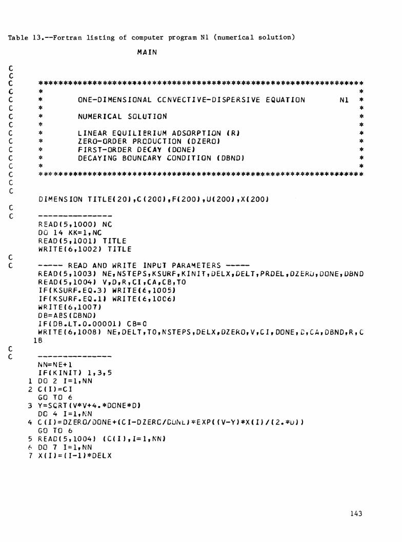
Table 13.—Fortran listing of computer program Nl (numerical solution)
MAIN
C C
C * * C * ONE-DIMENSIONAL CCNVECTIVE-DISPERSIVÊ EQUATION Nl * C * * C * NUMERICAL SOLUTION * C ♦ * C * LINEAR EQUILIBRIUM ADSORPTION ÍR) * C * ZERO-ORDER PRODUCTION (DZERO) * C * FIRST-ORDER DECAY (DONE) * C * DECAYING BOUNDARY CONDITION ÍDBND) ♦ C * * C *****♦♦****♦******♦«♦****♦♦******♦****♦****♦♦****♦*♦************** C C
C C
C C
DIMENSION TITLEÍ20),C(200),F(200),U{200J,XÍ200i
READ{5,1000) NC Dû 14 KK=1,NC READ(5,1001J TITLE WRITE(6»1002) TITLE
C C READ AND WRITE INPUT PARAMETERS
READ(5,1003) NE,NSTEPS,KSURF,KINIT,DELX,DELT,PRDêL,OZERU,OONE,üßND READÍ5,1004) V.D,R,CI ,CA ,CB,TO IF(KSURF.EQ.3) WRITEÍ6,1005J IFÍKSURF.EQ.ll WRITE(6,10C6) WRITE{6,1007J DB=AeS(CBNDi IFÍDB.LT.0.00001) CB=0 WRITE(6,1008) NE,DELT,T0,NSTEPS,DELX,DZER0,V,CI,D0NE,D,CA,D6ND,R,C
IB
NN=NE+1 IF(KINIT) 1,3,5
1 DO 2 1=1,NN 2 C(I)=CI
GO TO 6 3 Y=SCRT{V*V+4.*00NE*D)
DC 4 1=1,NN 4 C(I)=OZERO/uONE+(CI-DZERC/DüNLJ*EXP((V-Y)*X(I)/(2.*u))
GO TO 6 5 READ{5,1004) (C(I),1=1,NN) 6 DO 7 1 = 1,NN 7 X(I)=(I-1)*DELX
143

MAIN
V=V*OELT/DELX D=D*0£LT/DELX**2 RN=(R+0.5*DELT*OONE)/6. R0=(R-0.5*DELT*DONE)/6. DZERO=CZERO*D£LT DN=0-V*V/6. D0=D+V*V/6. EN=-0.5*DN+0.25*V+RN E0=0.5*D0-0.25*V+R0 BN=-0.5*DN-0.25*V+RN 60=0.5*00+0.2 5*V+K0 Uil)=0.5*DN+0.25*V+2.*RN IFÍKSÜRF.EQ.l) ü(l)=1.0 DN2=DN+A.*RN Dl=-0.5*00-0.25*V+2.*P0 02=-D0+4.*R0 BND=1.0 IF(DB.GE.O.OOOOl) BND=iEXPÍDBND*DELTJ-1.)/(DBND*DtLTJ IPRINT=PftDEL/OELT TIME=0.0 IF(KSURF.EQ.l) C(l)=Ci+CB KRITE(6,1009) TIME,(X(I),CíI),1=1,NNJ
C C DYNAMIC PART OF PRCGPAM
DO 12 II=l,NSTÊPS,IPkINT 0Ü 11 JJ=1,¡PRINT TIME=(II+JJ-1)*0ELT
IF(TIME.GT.T0J CA=0.0 IF(TIME.GT.TO} C3=0,0
C C CCNSTRüCT KNOWN VECTOR
EXT=CB*EXP(-OöNO*TIMEJ IFÍKSURF.EQ.li F(1J=CA+EXT IF(KSÜRF.EQ.3) Fí1)=D1*C(1J+E0*CÍ2)+0.5*D¿fcR0+V*ÍCA+BND*EXTJ DO 8 I=2»NE
8 F(IÍ=BO*C( I-1)+D2*C{IHE0*C(I + 1)+DZEK0 C C SOLVE FOR NEW VALLES
R=BN/U(I) F(2)=F(2)-R*F(1) IFÍKSÜRF.EQ.IJ R=0.0 U(2)=ÛN2-R*EN 00 9 1=3,NE R=bN/U(I-l) J(I)=0N2-R*EN
9 F<I)=F(I)-R*F(I-1) CÍNN)=F(N£)/(Ü(NE)+EN) DO 10 1=2,NN
144

MAIN
K=NN+1-I 10 C(K}=(f(K)-EN*C(K+1)}/U(K) 11 IF(KSüRF.EQ.l) C(1}=F(1) 12 WRITE(6,1009J TIME,(XÍI),C(I),1=1,NN) 14 CONTINUE
1000 FORMATdS) 1001 FORMAT (20A4) 1002 FORMAT(1H1,10X,82(1H*)/11X,1H*,80X,1H*/1IX,lH*,9X,'üNE-UlMfcNS10NAL
1 CONVECTIVE-OISPERSIVE EQUATION«,25X,1H*/11X,IH*,80X,1H*/11X,1H*,9 2X,«NUMERICAL SOLUTION« ,53X , 1H*/1IX ,iH*,SOX,1H*/11X,1H*,9X,« LINEAR 3EQUILIBRIUM ADSORPTICN (R) • ,38X,1H*/11X,IH*,9X,«ZERO-CRDER PRODUCT 4I0N (DZERO)«,42X,1H«/11X,1H*,9X,«FIRST-LkDER DECAY (DCNEJ«,47X,IH* 5/llX,lH*,9X,«DECAYING BOUNDARY CONDITION (DBND)«,37X,1H*/11X,1H*,8 60X,1H*/11X,1H*,20A4,1H*/11X,1H*,80X,1H*J
1003 F0RMAT(4I5,6F10.0) 1004 FORMAT(8F10.0) 1005 F0RMAT(11X,1H*,9X,«THIRD-TYPE BOUNDARY CONDITION«,42X,1H*J 1006 fÜRMAT(llX,lH*,9X,«FIRST-TYPE BOUNDARY CONDITION «,42X,IH*) 1007 F0RMAT(llX,iH»,80X,lH*/llX,82(lH*J) 1008 FCRMAT(//11X,« INPUT PARAMETERS«/11X,16(1H=}//IIX,« NE =«,oX,15,15X,
I'DELT =«,F9.4,15X,«TO =•,F11.4/11X,•NSTEPS =«,17,15X,«DELX =«,F9.4 2,15X,«DZERO =«,F8.4/11X,«V =•,F12.4,15X,«CI =«,Fil.4,15X,«DONE =«, 3F9.4/11X,«D =«,F12.4,15X,«CA =«,Fl1.4,15X,«DBND =«,F9.4/11X,«R =«, 4F12.4,15X,«CB =«,F11.4)
1009 F0RMAT(/llX,103ilH*)//llX,«CONCENTRATION AT TIME =«,F10.4//3X,5(8X 1,«DEPTH«,4X,'VALUE•)/(4X,5(2X,FIO.2,FIO.4J)) STOP END
145

Table 14.—Sample output from computer program Nl (numerical solution)
ONE-DIMENSIûNAL CONVECTIVE-CISPEKSIVE EQUATION
NUMERICAL SOLUTION
LINEAR EQUILIBRIUM ADSCRPTICN ÍR) ZERO-ORDER PRODUCTIÜN (OZEROJ FIRST-ORDER DECAY (DCNE) DECAYING BOUNDARY CCNDITIGN (DBND)
EXAMPLE A3-1 (P=5)
FIRST-TYPE BOUNDARY CONDITION
4c4c3»c4c:tc;(c4c:(c]tc;ec:^;«c:tc:tc4c4c:«:4c4(«4c«*«:|c«4c«:4c*3('*«4'«4c:^4c4c4c4c4c«4'4'4':t'«:tc4c^4t««4c:Ct4c«*«*
INPUT PARAMETERS = = =: = == = :
NE =
r = = = = = =
40 NSTEPS = 125 V = l.COOO D = 4,0000 R = 1.0000
OELT = 0.2000 DELX = 0.5000 CI = 0.0 CA = 1.0000 CB = 0.0
TO = iOOO, ► 0000 DZERO = 0, .0 DÜNE • 0, ► 0
DBND = 0, .0
««#4c:(c:^4c^4c;ic4c«4c4c:^4c4(4(«<(«:0c^4c4(4(«4(«4c«3^**:((*«4>««4c««««4(*«**4c4c:(c^««4c««««:(c4c34(:4c4e^^^
CONCENTRATUN AT TIME = 0.0
DEPTH VALUE DEPTH VALUE DEPTH VALUE DEPTH VALUE DEPTH VALUE 0.0 1.0000 0.50 0.0 1.00 0.0 1.50 0.0 2.00 0.0 2.50 0.0 3.00 0.0 3.50 0.0 4.00 0.0 4.50 0.0 5.00 0.0 5.50 0.0 6.00 0.0 6.5Û 0.0 7.00 0.0 7.50 0.0 8.00 0.0 8.50 0.0 9.00 0.0 9.50 0.0
10.00 0.0 10.50 0.0 11.00 0.0 11.50 0.0 12.00 Û.Û 12.50 0.0 13.00 0.0 13.50 0.0 14.00 0.0 14.50 0.0 15.00 0.0 15.50 0.0 16.00 0.0 16.50 0.0 17.00 0.0 17.50 0.0 18.00 0.0 18.50 0.0 19.00 0.0 19.50 0.0 20.00 0.0
:ec4c4c:^4c4c4t4t4c4c4c<t4cX«4c4e«4c4c:tc4c4c4c;|í4'4c4c4c««««*4i4'«*«««**««««*4(«««*«4(4c4e]4c4c:t(^]»c:tc9tc*3((4(4c#
CONCENTRATICN AT TIME 5.00CC
DEPTH VALUE DEPTH VALUE DEPTH VALUE DEPTH VALUE DEPTH VALUfc 0.0 l.COOO 0.50 0.S818 1.00 0.9532 1.50 0.9346 2.00 0.9019 2.50 0.8750 3.00 0.8424 3.50 0.8089 4.00 0.773o 4.5ü 0.7372 5.00 0.6Ç95 5.50 0.6610 6.00 0.6219 6.50 0.5626 7.00 0.543^ 7.50 0.5043 8.00 0.4659 8.50 0.4285 9.00 0.3921 9.50 0.3570
10.00 0.3235 10.50 0.2917 11.00 0.2616 11.50 0.2334 12.00 0.¿07¿ 12.50 0.1830 13.00 0.1608 13.50 0.1405 14.00 0.1221 14.50 O.i03o 15.00 0.0909 15.50 0.C779 16.00 0.0666 16.50 0.05ö7 17.00 O.Û4dJ 17.50 0.0413 18.00 0.0357 18.50 0.0313 19.00 0.02äj 19.50 0.02oä 20.00 0.0268
illi:^:tL:^:^tf:^^^itli:íti:i,:^^4iiii^i:^:^:ii,:ii:t,:t^:^^:tt.^,^^:t,:^t*************A'******'>i*
CONCENTRATION AT TIME = lO.OOOC
146

DEPTH VALUE DEPTH VALUE DEPTH VALUE DEPTH VALUE DEPTH VALUE 0.0 1.0000 0.50 0.9920 1.00 0.9835 1.50 0.9733 2.00 0.9628 2.50 0.9506 3.00 0.9379 3.50 0.9237 4.00 0.9087 4.50 0.8926 5.00 0.6754 5.50 0,8572 6.00 0.tí380 6.50 0.8178 7.00 0.7968 7.50 0.7750 8.00 0.7524 8.50 0.7291 9.00 0.7052 9.50 0.6807
10.00 0.6559 10.50 0.63C8 11.00 Ü.6054 11.50 0.5800 12.00 0.5546 12.50 0.5294 13.00 0.5045 13.50 0.4800 14.00 0.4561 14.50 0.4330 15.00 0.4107 15.50 0.3896 16.00 0.3697 16.50 0.3514 17.00 0.3347 17.50 0.3200 18.00 0.3C75 18.50 0.2976 19.00 0.2906 19.50 0.2869 20.00 0.2869
4c#4c4í4c:(c«4c4c:tc4c4c4c:tc4c:t(«4c4c:«c4c4c4c«*4c4(4c4c4c*4t4'****:tc4(4c4c4c4c*4c*:tc:4(«:tc«««:4c:tc4c««4c««4c4c4c4^
CONCENTRATION AT TIME = 15. .0000
DEPTH VALUE DEPTH VALUE DEPTH VALUE DEPTH VALUE DEPTH VALUE 0.0 1.0000 0.50 0.9962 1.00 0.9919 1.50 0.9872 2.00 0.9819 2.50 0.9761 3.00 0.9697 3.50 0.9628 4.00 0.9553 4.50 0.9472 5.00 0.9384 5.50 0.9290 6.00 0.9190 6.50 0.9084 7.00 0.8972 7.50 0.6653 8.00 0.8729 8.50 0.8599 9.00 0.8463 9.50 0.8322
10.00 0.8176 10.50 0.8026 11.00 0.7873 11.50 0.7716 12.00 0.7556 12.50 0.7395 13.00 0.7234 13.50 0.7072 14.00 0.6912 14.50 0.6755 15.00 0.6601 15.50 0.6453 16.00 0.6312 16.50 0.6180 17.00 Û.6Û60 17.50 0.5952 Ic.OO 0.5861 18.50 0.5787 19.00 0.5735 19.50 0.5707 20.00 0.5707
^(♦4c«*«4c4c«4c4(4c4c4c4(*«4'4í«««4t*«**«4í4(*4(««**««4c*3ic4c«4(*4(«««**«*4(*«*:«c«***4e««4c««««4(4(**«««
CONCENTRATION AT TIME = 20. .OOOC
DEPTH VALUE DEPTH VALUE DEPTH VALUE DEPTH VALUE DEPTH VALUfc 0.0 1.0000 0.50 C.9980 1.00 0.9958 1.50 0.9933 2.00 C.99Û5 2.50 0.9875 3.00 0.9641 3.50 0.9804 4.00 0.9764 4.50 0.9721 5.00 0.9674 5.50 0.9624 6.00 0.9570 6.50 0.9513 7.00 0.9452 7.50 0.9387 8.00 0.9319 8.50 0.9247 9.00 0.9172 9.50 0.9093
10.00 0.9012 10.50 0.8927 11.00 0.8840 11.50 0.8751 12.00 0.8660 12.50 0.8567 13.00 0.8474 13.50 0.8380 14.00 0.8287 14.50 0.8194 15.00 0.8104 15.50 0.8017 16.00 0.7934 16.50 0.7855 17.00 0.77b4 17.50 0.7719 18.00 0.7665 18.50 0.7621 19.00 0.7589 19.50 0.7i)7^ 20.00 0.7573
tL:ti*:t^:^^ti:^^m*****^^**********m****T^****^***^**i^*******^^****^4^^****^*****'t^
CONCENTRATION AT TIME = 25, • OOOC
DEPTH VALUE DEPTH VALUE DEPTH VALUE DEPTH VALUE DEPTH VALUc 0.0 1.0000 0.50 0.S989 1.00 0.9977 1.50 0.9964 2.00 0.9949 2.50 0.9932 3.00 0.9914 3.50 0.9894 4.00 0.9872 4.50 0.9849 5.00 0.9823 5.50 0.9796 6.00 0.9766 6.50 0.9735 7.00 0.9702 7.50 0.9666 8.00 0.9629 8.50 0.9589 9.00 0.9548 9.50 0.9504
10.00 0.9459 10.50 0.9413 11.00 0.9364 11.50 0.9315 12.00 0.9^04 12.50 0.9212 13.00 0.916C 13.50 0.9108 14.00 0.9056 14.50 0.9004 15.00 0.8953 15.50 0.8904 16.00 0.8858 16.50 0.8814 17.00 0.8773 17.50 0.8737 18.00 0.8706 18.50 0.8681 19.00 0.8664 19.50 0.8654 20.00 0.8654
147

i^^i^:ííi:¡^:i^z(f4^i^ir^iíii(li^i)lii^T^7^:^tíi:i(f.^:¡íi:ii:^:^i(^:t^:^li1^^:^4*^***^**^
GNE-DIMENSICNAL CONVECT IVE-CISPERSI VE EQüATIC.>í
NUMERICAL SOLUTION
LINEAR EQUILIBRIUM ADSCRPTICN (R) ZERO-CRDER PRODUCTION ÍOZEPCJ FIKST-OROER DECAY (DONE) DECAYING BOUNDARY CONDITICN (06ND)
EXAMPLE B14-1
THIRD-TYPE BOUNDARY CCNDITICN
:¡lí4i1lii:(f:tlc:t^4ii^í:t^it::ti::ili:t,:i,:i^i(lti(li^:^:1^ilf:tii(lL4,:lli:^f:tíilíi^:tf 4***4******^*
INPUT PARAMETERS
NE = 40 NSTEPS = 125 V = 25.0000 D = 37.5000 R = 3.0000
DELT = 0.1000 DELX = 2.5000 CI = 0.0 CA = 0.0 CB = 10.0000
TO = 1000. .0000 JZERO = 0, .5000 DONE = 0, .0 OBND = 0, .2500
4c«:(cjtc:tc;(c«4c4c«;«c4e]ic:^^4c:(c:«c^X'3(c«3(c4c4'«*4(4c^««««4c««<(:(c4c4(:^«*4c4c*3»e4(4(4'4e4'««4c4c4c4c4c«4c«
CCNCENTRATICN AT TIME = 0.0
DEPTH VALUE DEPTH VALUE DEPTH VALUE DEPTH V>4LJt DEPTH VALUc 0.0 0.0 2.50 0.0 5.00 0.0 7.50 Ö.Ü 10.00 0.0
12.50 0.0 15.00 0.0 17.50 Û.0 20.00 0.0 22.50 0.0 25.00 0.0 27.50 0.0 30.00 0.0 32.50 0.0 35.00 0.0 37.50 0.0 40.00 0.0 42.50 0.0 45.00 0.0 47.50 0.0 50.00 0.0 52.50 0.0 55.00 0.0 57.50 0.0 60.00 0.0 62.50 0.0 65.00 0.0 67.50 0.0 70.00 0.0 72.50 0.0 75.00 0.0 77.50 0.0 80.00 0.0 82.50 0.0 85.00 0.0 87.50 0.0 90.00 0.0 92.50 0.0 95.00 0.0 97.50 0.0 00.00 0.0
i^^:t^^,^,:^^:lí,l,iiii,l¡:4,^:t^:^jt^:t^:^:tí^^ci^:t^^Mf4i:tí********************4í****^*****^
CONCENTRATION AT TIME = 2, ,5C0C
DEPTH VALUE DEPTH VALUE DEPTH VALUE DEPTH VALUE DEPTH VALUE 0.0 5.6214 2.50 6.C918 5.00 6.5153 7.50 6.8443 10.00 7.0058
12.50 6.9274 15.00 6.5612 17.50 5.9075 20.00 5.0253 22.50 4.0^29 25.00 3.0287 27.50 2.1557 30.00 1.4732 32.50 0.9977 35.00 0.7032 37.50 0.5420 40.00 0.4646 42.50 0.4323 45.00 0.4209 47.50 0.4176 50.00 0.4168 52.50 0.4167 55.00 0.4167 57.50 0.4167 60.00 0.4167 62.50 0.4167 65.00 0.4167 67.50 0.4167 70.00 0.4167 72.50 0.4167 75.00 0.4167 77.50 0.4167 80.00 0.4167 82.50 0.4167 85.00 0.4167 87.50 0.4167 90.00 0.^167 92.50 0.4167 95.00 0.4167 97.50 0.4167 100.00 0.4167
«4c4c4c*44c«**^««4c4(«4(4(^«4c4c*4c4(«««*«**««*««««*4c*«*«««*4c«#«*«4(4c4c4c««4(««#«4(4c««4(4(«4(^**
CONCENTRATION AT TIME = 5.000C
148

NATIONAL AGRICULTURAL LIBRARY
1022423354
DEPTH VALUE DEPTH V/iLUE DEPTH VALUE DEPTH VALUE DEPTH VALUE 0.0 3.0357 2.50 3.3312 5.00 3.6457 7.50 3.9792 10.00 4.3305
12.50 4.6959 15.00 5.0667 17.50 5.43 76 20.0Û 5.7861 22.50 6.0926 25.00 6.3309 27.50 6.4737 30.00 6.495Ö 32.50 6.3787 35.00 6.1138 37.50 5.7144 40.00 5.1972 42.50 4.5993 45.0Ü 3.9636 47.50 3.3342 50.00 2.7500 52.50 2.2399 55.00 1.8199 57.50 1.4935 60.00 1.2539 62.50 1.0880 65.00 0.9795 Ö7.50 0.9127 70.00 0.8740 72.50 0.85^9 75.00 0.8422 77.50 0.8371 80.00 0.8348 82.50 0.ö338 85.00 0.8335 87.50 0.8334 90.00 0.8333 92.50 0.8333 95.00 0.8333 97.50 0.833J
100.00 0.8333
:tc4c««4c*«*4c«4c*4c*«4c4'«*«4'««««#«4c4c4c4t4c«4(**«*4c4c«:tc4c4c4>««4c*««4(#«««*4c«4(*«4c:(i«;»4c4c*«**«*«
CONCENTRATION AT TIME = 7, 500C
DEPTH VALUE DEPTH VALUE DEPTH VALUE DEPTH VALUE OtPTH VALUE 0.0 1.6389 2.50 1.8207 5.00 2.0132 7.50 2.2174 10.00 2.4340 12.50 2.6641 15.00 2.9C8^ 17.50 3.1675 2Û.Û0 3.4418 22.50 3.7311 25.00 4.0343 27.50 4.3491 30.00 4.6715 32.50 4.9954 35.00 5.31^4 37.50 5.6117 40.00 5.6800 42.50 6.1026 45.00 6.2641 47.50 6.3303 50.00 6.3494 52.50 6.2541 55.00 6.0628 57.50 5.7805 60.00 5.4191 62.50 4.9959 65.00 4.5326 67.50 4.0528 70.00 3.5794 72.50 3.1327 75.00 2.7285 77.50 2.3772 80.00 2.0837 82.50 1.8476 85.00 l.oö4^ 87.50 1.5287 90.00 1.431C 92.50 1.3636 95.00 1.3187 97.50 i.2ö98 00.00 1.2898
4(«4c4c4c4'«4c4(:tc#4(**4t4c«*««4c4'*4c***4c«*«*««««*«*«4(4(««««*«*4c4(««*«««#«4(««4í««««******^«*««4c*
CONCENTRATION AT TIME = 10, 0000
DEPTH VALUE DEPTH VALUE DEPTH VALUE DEPTH VALUE DEPTH VALUE 0.0 0.8912 2.50 1.0117 5.00 1.1380 7.50 1.2706 10.00 1.4099 12.50 1.5565 15.00 1.7111 17.50 1.8741 20.00 2.0464 22.50 2.22Ö6 25.00 2.4214 27.50 2.6255 30.00 2.8415 32.50 3.0700 35.00 3.3112 37.5D 3.5651 40.00 3.8310 42.50 4.1077 45.00 4.3930 47.50 4.6834 50.00 4.9743 52.50 5.2597 55.00 5.5319 57.50 5.7823 60.00 6.0011 62.50 6.1782 65.00 6.3039 67.50 6.3694 70.00 6.3683 72.50 6.2965 75.00 6.1536 77.50 5.9^29 80.00 5.6716 82.50 5.3498 85.00 4.9907 87.50 4.6088 90.00 4.2191 92.50 3.8358 95.00 3.4720 97.50 3.1540 00.00 3.1540
*^^iiti^:tí4i}l^illiiliWiitL^:tí:ti4i:tití:ti$ií^:^^i^^:^^jfli^t**4******'^*****^***********
CONCENTRATICN AT TIME = 12, ,5000
DEPTH VALUE DEPTH VALUE DEPTH VALUE DEPTH VALUE DEPTH VALUE 0.0 0.4910 2.50 0.5767 5.00 0.6696 7.50 0.7638 10.00 0.8616 12.50 0.9633 15.00 1.C693 17.50 1.179a 20.00 1.2953 22.50 1.4162 25.00 1.5428 27.50 1.6758 30.00 1.8155 32.50 1.9625 35.00 2.1173 37.50 2.2807 40.00 2.4530 42.50 2.6350 45.00 2.8271 47.50 3.0299 50.00 3.2436 52.50 3.4663 55.00 3.7037 57.50 3.9494 60.00 4.2039 62.50 4.4656 65.00 4.7316 67.50 4.9985 70.00 5.2618 72.50 5.516Ü 75.00 5.7548 77.50 5.9715 80.00 6.1587 82.50 6.3092 85.00 6.4162 87.50 6.4739 90.00 6.4781 92.50 6.4265 95.00 6.3216 97.50 6.1898 00.00 6.1898
149