IGVC2015-MANTIS 2.0

THE MANTIS 2.0 INTELLIGENT ROBOTIC PLATFORM

Oakland University

Brian Neumeyer, Jozefina Ujka, Tyler Gnass, Parker Bidigare, Christopher Hideg, Lucas Fuchs, Sami Oweis Ph.D., Hudhaifa Jasim

Ka C Cheok Ph.D. Micho Radovnikovich Ph.D.

ABSTRACT

This paper presents the Mantis 2.0 robotic platform developed to compete in IGVC for 2015. Innovations

in the electrical system include custom designed and fabricated H-bridges, and a custom embedded microcontroller board, in addition to the removable housing and controllers with military grade connectors. Innovations in the software system include multi-rate Kalman pose estimation, effective interpretation of stereo vision data, fusion of LIDAR with monocular cameras, line fitting with the RANSAC algorithm, 3D map-based path planning, and the ability to create and load reusable maps of the environment.

INTRODUCTION

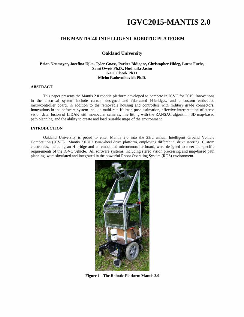
Oakland University is proud to enter Mantis 2.0 into the 23rd annual Intelligent Ground Vehicle Competition (IGVC). Mantis 2.0 is a two-wheel drive platform, employing differential drive steering. Custom electronics, including an H-bridge and an embedded microcontroller board, were designed to meet the specific requirements of the IGVC vehicle. All software systems, including stereo vision processing and map-based path planning, were simulated and integrated in the powerful Robot Operating System (ROS) environment.

Figure 1 - The Robotic Platform Mantis 2.0

Figure 3 - CAD rendering of 'Mantis 2.0

DESIGN PROCESS

A classic ‘V-Model’ design process was followed to develop Mantis 2.0, shown in Figure 2. After defining the requirements of Mantis 2.0, a design was formed using CAD, and a detailed simulation environment was formed to develop the navigation system, see Figure 3. After implementing the design and integrating the various components, a rigorous test cycle began, where consistent failure points were identified and rectified through minor adjustments or larger design changes.

Figure 2 - The design process used to build Mantis 2.0

MECHANICAL DESIGN

At the beginning of the design phase, based on past IGVC experience, it was mandated that Mantis 2.0 must be able to perform a zero-point turn. This capability greatly simplifies the path planning and control. The simplest and most widely used drive method that enables zero-point turns is differential steer. Additionally, differential steer simplifies the mechanical aspects of the drive train, since it operates solely on wheel rotation, and does not require any additional moving parts.

An electric wheelchair, shown in Figure 4, was selected as the platform due to its durability, suspension, and interfacing capabilities. Using a medical grade drivetrain has proven beneficial in its reliability. Limiting vibrations to the electronics and sensors on board was a concern. The wheelchair’s unique rocker suspension contains two independent links that suppress vibration and large impulses. Two centrally driven tires with four supporting castors create a tight turn radius with the turn axis in the center of the footprint. The wheels are driven by brushed DC motors. The top of the wheelchair base is a flat mounting surface with an existing bolt pattern.

The superstructure mounted on top of the wheelchair base provides a waterproof enclosure for the laptops and electronics. The cameras are mounted angled downwards near the top to maximize the field of view. Additional cameras are mounted at half height on either side to add close range and side visibility. The GPS antenna is mounted at the very top positioned over the drive wheels. The LIDAR sensor is mounted center front to get 240 degrees of visibility, shown in Figure 5.

Fig 5. Enclosed LIDAR a Fig. 4 - The wheelchair base for Mantis 2.0

The superstructure frame is composed of 1”x1” extruded aluminum tubing with a 1/16th thick wall. Aluminum was selected for its low density and high strength to mass ratio. Individual tubes are riveted together so if a part needs to be replaced it can be easily drilled out and substituted. The steel rivets keep structural integrity and prevent the frame from flexing while preventing the permanent and cumbersome disadvantages of welding and bolting. The light aluminum superstructure, the wheelchair base contributes the majority of the mass. This places the center of mass in the center of the drive wheels, about 6 inches above the ground.

ELECTRONIC COMPONENTS

Mantis 2.0 is designed with a fully modular electronics bay, shown in Figures 7 and 8. This efficient design

allows for the main power systems to be separated from the chassis via series a of easy disconnects. The main power systems of the robot include circuit breakers, solid state relays, H-bridges, and drive controls.

Figure 7 - Electronics Box Rear. Figure 8 - Electronics Box Front

The electrical connections were military grade connectors, were used for higher durability, see Figures 9a and 9b. The removable electronics allows for easy off- chassis integration, diagnostics and testing. The connectors were set at both sides of the electronic bay; they were identified per connector and based on I/O numbers for universality between the power and load distributions.

Figure 6 - Mechanical Suspension

Figure 12: Novatel GPS

a). b).

Figure 9 a & b: Both sides of the suitcase connectors

The connectors were installed by different IO headers for each

feature; such as 2-Pin headers for LED, 4-Pin headers for Switches. Some were set using different genders for the connectors, this provided protection and consistancy. See Figures 10.

Mantis 2.0’s H-bridges are completely custom-designed PCBs. Based on past experience with other H-bridges such as IFI’s Victor series, it was desired to use an H-bridge that is more flexible, robust, and capable of chopping the motor power at a much higher frequency. A conventional single-channel PWM signal controls the speed and direction of the H-bridge output.

Key features of the H-bridges shown in Figure 11 are:

● On-board fuses ● Automatic fan control ● Reverse battery protection ● Over-current protection ● Over-temperature protection ● Serviceable components

Mantis 2.0 is equipped with an array of sensors that allow it to

detect obstacles, compute its location, heading, speed, and be operated in a safe and reliable manner. All the sensors make it possible for Mantis 2.0 to locate itself and have a high precision when maneuvering.

The sensor array consists of:

● NovaTel FlexG2-Star GPS receiver

○ 8 Hz, less than 1 meter accuracy, shown in Figure 12. ● 4 uEye UI-2220SE color USB 2.0 Cameras

○ 768x576 resolution, ½” CCD sensor, 50 Hz, also shown in Figure 12. ● Hokuyo UBG-04LX LIDAR sensor

○ 4 meter range, 240 degree field of view, 35 Hz, shown in Figure 5 (above). ● InvenSense ITG-3200 tri-axis gyro, integrated shown in Figure 13. ● Honeywell HMC5843 tri-axis magnetometer, integrated shown in Figure 13. ● US Digital E3 Wheel 2500 CPR encoders ● DX6i wireless R/C aircraft joystick

o Embedded controller-based manual control and wireless E-stop

Figure 10: Modular design in the connector headers

Figure 11 - H-Bridge Sensors

Drive Control Board

The embedded controller board is a custom PCB that was designed specifically for Mantis 2.0. The motivation to do so resulted from using off-the-shelf FPGA and microcontroller development boards in the past which were not specifically designed for the application, shown in Figure 13. The embedded control board is designed to satisfy all hardware needs, and provide the flexibility of a commercially available development board without the extra bulk and space of unused functionality.

Key features of the embedded control board are:

● 32-bit Microchip PIC microprocessor ● Dedicated hardware quadrature counters to efficiently

perform high-resolution encoder data processing ● Integrated accelerometer, gyro, and magnetometer for robust

robot pose estimation ● High speed USB communication ● Battery voltage monitoring ● Power switches and distribution ● General I/Os, input capture, PWM

Power Distribution

Figure 14 shows a block diagram of Mantis 2.0’s power distribution system. The power for the robot comes from two 12V AGM batteries, wired in series to make a 24V system. The entire electrical system is routed through a main circuit breaker for protection. The operator has the ability to power-up the embedded control board and sensors separate from the H-bridges for testing and safety purposes. The H-bridges are driven through dual custom solid state relay PCBs for redundancy. The relay boards are galvanic isolated preventing incorrect ground return paths from occurring. The batteries can be conveniently charged on-board, or quickly replaced by another set to achieve optimal runtime.

Power and ground were distributed using two terminal rails; one for power and other was for ground. This allows an even distribution for both common ground and power among the elements of the electronic bay.

Figure 14 - Power Distribution System.

Figure 13- Custom Embedded Controller Board.

Safety Considerations

Many precautions were taken into account when designing Mantis 2.0's emergency stop system. In addition to two conventional turn-to-release E-stop switches, shown in Figure 15, a DX6i joystick is used for disabling the motor output wirelessly. The DX6i has a range of several hundred feet. To protect against a variety of failure conditions, the drive control system automatically turns off the motors if it fails to receive commands from the computer or joystick after 200ms. A Figure 15 - Emergency stop

COMPUTING HARDWARE Embedded Controller

The microcontroller runs a Real-Time Operating System (RTOS) to manage its tasks. Data from the inertial sensors is gathered at a rate of 200Hz and streamed to a laptop using custom USB drivers.

Closed loop velocity control is critical to accurately follow a plan generated by higher level software.

Closed loop velocity PI controllers were implemented on the embedded microcontroller for each wheel. The control loop is the highest priority task in the operating system of the microcontroller, and runs at 100 Hz. The velocity feedback is reported to higher level software for localization. Velocity commands come from higher level software and the DX6i wireless joystick.

Laptop Computers

All high-level processing is performed on two Lenovo Thinkpad W530 laptops. Their processor is a quad

core, 3.4 GHz Intel i7, and has 16 GB of RAM. To make the laptops robust to the vibration encountered on a ground vehicle, a solid state drive is used instead of a conventional hard disk drive. The operating system is Ubuntu 14.04, and runs the “I” distribution of ROS. An ethernet switch manages the communications between all the devices.

ROS SOFTWARE PLATFORM

Mantis 2.0's software systems are implemented on the Robot Operating System (ROS) platform. ROS is an

open-source development environment that runs in Ubuntu Linux. There is a multitude of built-in software packages that implement common robotic functionality. Firstly, there are many drivers for common sensors like LIDAR, cameras and GPS units. There are also general-purpose mapping and path planning software modules that allow for much faster implementation of sophisticated navigation algorithms.

Efficient Node Communication

A ROS system consists of a network of individual software modules called “nodes”. Each node is

developed in either C++ or Python, and runs independently of other nodes. Communication messages between nodes are visible to the entire system similar to an automotive CAN bus. Inter-node communication is made seamless by a behind-the-scenes message transport layer. A node can simply “subscribe” to a message that another node is “publishing” through a very simple class-based interface in C++. This allows for the development of easily modular and reusable code, and shortens implementation time of new code.

Debugging Capabilities

One of the most powerful features of ROS is the debugging capability. Any message passing between two

nodes can be recorded in a “bag” file. Bag files timestamp every message so that during playback, the message is recreated as if it were being produced in real time. This way, software can be written, tested and initially verified without having to set up and run the robot.

Bag playback is especially helpful when testing the mapping and vision algorithms to visualize and reproduce

failure cases.

Another convenient debugging feature is the reconfigure GUI. This is an ROS node that allows users to change program parameters on the fly using graphical slider bars. This tool is invaluable, since most robotic vehicle controllers require precise adjustment of several parameters, and being able to change them while the program is running is very beneficial.

Simulation

Gazebo is an open source simulation environment with a convenient interface to ROS. To rigorously test

Mantis 2.0’s artificial intelligence, simulated IGVC courses were constructed. These courses contain models of commonly encountered objects: grass, lines, barrels, and sawhorses. The configurations are designed to emulate the real IGVC course as accurately as possible. The simulation environment proved invaluable to the development process, since, unlike recorded data, the simulation responds to robot decisions and generates appropriate simulated sensor data.

Figure 16- Block Diagram of the Vision System Modules.

Figure 16 provides a block diagram overview of the vision pipeline. A front facing stereo camera pair, left and right side short range monocular cameras, and a LIDAR scanner comprise the sensors utilized by the vision system. From the stereo pair input, the stereo matcher feeds the plane extractor with 3D point cloud data that is filtered by the plane extractor into domain specific height data used by the flag and line detection units. The line detector additionally uses the short range monocular cameras fused with the LIDAR to compensate for blind spots left by the narrow field of view of the front facing stereo pair. The flag and line point clouds outputs are inputs to the navigation system.

Stereo Vision

Most LIDAR sensors can only detect objects on one plane. At past competitions, this limitation caused problems, especially in the case of the sawhorse-style obstacles, seen in the foreground of the image in Figure XX. The horizontal bar of the obstacle would not be in the scan plane, thereby going undetected, and the vehicle would frequently try to fit between the two legs of the obstacle.

Mantis 2.0 addresses this severe sensor limitation by using stereo vision. Applying open-source functions for

stereo image matching, the images from the stereo camera pair are processed to generate a 3D cloud of points corresponding to everything in the frame.

The two stereo cameras are mounted eight inches apart near the top of the robot. The image capture is

hardware synchronized to make sure the left and right images are always matched, even at high speeds. Some obstacles of uniform color do not have enough texture to find confident matches between images. Because of this, data near the center of the uniform obstacles tends to be absent, while edges, grass, and everything else is reliably detected and mapped to a 3D point.

Figure 9 shows an example image and the corresponding point cloud. Each point in the cloud is marked with

the color of the image pixel is corresponds to. On top of the point cloud is LIDAR data, indicated by the yellow squares. This example shows how much information the LIDAR misses in certain situations, and exemplifies the capabilities of a carefully implemented stereo vision system.

Automatic Camera Transform Calibration

To calibrate the transform from the cameras to the ground, an automatic algorithm was developed using a

checkerboard. Assuming the checkerboard is flat on the ground, the 48 vertices in an 8x6 grid are optimally fitted to a plane equation to detect the camera position and orientation. This transform is used to place stereo and LIDAR data on the map from different coordinate frames. Figure 10 shows an example of how the transform calibration is performed on a real image. The calibration algorithm has proven to be very reliable and yields very accurate point clouds.

Figure 19 - Example of the Automatic Transform Calibration Procedure.

Figure 18 – Example Stereo Point Cloud and LIDAR Scan

Figure 17 - Dual cameras

Plane Extraction

The plane extractor is responsible for analyzing the raw point cloud output from the stereo matching algorithm. The goal is to generate images that contain only pixels within a certain height window, and black out the rest. Specifically, the two planes of interest are the ground plane, where the lines will be detected, and the flag plane, which is used for the flag detection algorithm. The height window to detect points on the ground plane is adjusted according to experimental results, and the height window for the flags is set according to the expected height of the flags on the course.

Additionally, the height information of obstacles is used to eliminate obstacle pixels from the generated ground plane image in order to make the line detection algorithm more robust. Figure XX shows examples of ground plane image generation, where pixels corresponding to points above the ground are blacked out, as well as regions of the ground pixels that correspond to where objects meet the ground. Notice how the resulting image primarily contains just grass and line pixels.

a) Simulated Images

b) Real Images

Figure 20 a & b - Example ground plane images in simulated and real scenarios.

LIDAR-Image Fusion

LIDAR data is used to remove objects from the monocular camera images. Each LIDAR point is projected onto an image using the known geometric transform and camera intrinsic parameters. Each projected point creates a vertical black line, resulting in an image with only pixels near the ground and black everywhere else. The final output is similar to the output of the plane extraction algorithm. Line Vision

Based on our previous experience in designing lane detection algorithm for the IGVC path, we had always encountered the problem of noisy images. The noise in the images; represented by ‘dead grass’ for example, makes it almost impossible to design a robust algorithm to detect the while lane without being affected by the noise. Consider the following samples of raw images that makes the usage of traditional image processing technique so complicated to detect the while lines only.For the reasons mentioned above, we have concluded that we need an intelligent and self-learning algorithm to detect while lines with less sensitivity to the noise. The Artificial Neural Networks have been used to training our robot to extract while lines in the image and discard most of the white noise in the image.

Fig 21. Line detection

Every neural network has a learning algorithm, which modifies and tunes the weights of the network. The self-tuning of the ANN is related to the learning function that measures the error in the prediction of the network. The learning algorithm in this case is the 'mean least square', in which the network tries to minimize the error to achieve the target error based on the features we pass to the network. This technique of learning is called a supervised learning, which occurs on every epoch (cycle) through a forward activation flow of outputs. The equation we have used in this assignment can be characterized as shown below:

Fig 22. Training process flow

Prediction

Every received raw image is divided into a set of sub-images. Every sub-image is passed to the ANN model to predict the label it belongs to. The returned parameter from the prediction algorithm is a vector, whose length equals the number of the labels. Every index of the label has a value that indicates the likelihood that image belongs to that label. The label that has the maximum value is the winner label. If the winner label is a white line, a point is recorded into a vector of points to be published to the navigation algorithm. Remarks

The problem we find the most complicated is to distinguish between a white line and the edge of the whole barrel. Given that our training data is mainly describe the while line as a set of connected white pixels grouped next to a set of connected green pixels. All the characteristics mentioned above to create the while line model apply exactly to the edge of a white barrel on a green grass.

Fig 23. Vision logical flow

Figure 27 - Diagram of the

Navigation System.

Figure 26 - Example Flag Negotiation Logic.

Model fitting is especially effective with dashed lines, occlusions, and gaps. Even though parts of the line may be missing, the parts all fit a single 2nd order polynomial model. Other approaches such as clustering would separate each piece and leave gaps. Figure 12 shows an example scenario where a barrel blocks part of the line from view, however RANSAC was able to fit a 2nd order polynomial to the line and fill in the gap. In the figure, blue is LIDAR data, red is the projection of all pixels determined to be close to white, and green is the optimal model fit output.

Figure 25 - RANSAC Block Diagram

Flag Detection

The flag plane image from the

input is fed to the flag detector. In this image, red and blue flags are separated by thresholding hue. To direct the robot towards the correct path, artificial lines are drawn on the map. Red flags draw to the right, and blue flags draw to the left. This blocks invalid paths and funnels the robot into the correct path. Figure 13 shows a simulated flag scenario illustrating this approach, where artificial lines are shown in white.

F

Figure 24 - Example Lane Detection RANSAC Model Fit

Figure 29 - Example of Global Plan Computed from 3D Map.

Figure 28 - Example of the Mapping Procedure.

NAVIGATION SYSTEM Kalman Filtering

The Kalman Filter fuses data from many sensors to accurately estimate position and orientation. Each sensor updates at a different rate, and the filter updates with the fastest sensor, 200Hz. This results in accurate dead- reckoning between slow GPS updates. To avoid the discontinuity of traditional Euler angles, the orientation is represented using a quaternion. In the two dimensional case, the yaw angle can be represented by a 2D vector. Figure 27 shows information about the sensors being fused together, and which state variable each is measuring.

Mapping

The Kalman Filter was found to be accurate enough to build a map without Simultaneous Location and

Mapping (SLAM). SLAM requires a cluttered environment to match incremental data, but obstacles on the IGVC course are relatively sparse.

Mantis 2.0's mapping algorithm places time-stamped

information on the map using the Kalman estimated position and orientation. The map is represented in 3D as 5 planar layers. Object information from three sources is placed on the map: 3D stereo data, LIDAR data, and detected lines. Line data is on the ground plane, LIDAR data is parallel to the ground plane and elevated, and 3D stereo data is present in all heights.

Each sensor can mark and clear space on the map.

Clearing is done by tracing a ray through 3D space from the sensor source to the obstacle, and clearing every cell in that path. Two instances of the mapping algorithm, global and local, run in parallel. The local map is a 15 meter square with 5 cm resolution. The global map is a 100 meter square with 10 cm resolution. The global map can be initialized a priori with a map generated from a previous run.

Global Path Planning

The global planner uses the global map to select the path to a

goal point with minimum cost. The occupied squares on the map are inflated using the robot’s width and an exponential cost function. The global planner is not allowed to plan a path passing through any inflated square.

Furthermore, the cost function allows the path planner to

choose the optimal path, even in both cluttered and open environments. The global planner implements Dijkstra's algorithm, and is an open-source package built in to ROS.

Figure 17 shows an example of a global path output from the

planner. The differently colored cubes represent the different layers of the 3D voxel grid map. The orange squares represent the inflated 2D projection of the 3D voxels onto the ground plane.

Reactionary Avoidance

Reactionary avoidance uses the local map to avoid collisions. This is the last stage in the path planning, and is responsible for overriding commands that would cause a collision. Future collisions are detected by simulating trajectories along evenly spaced turning radii. The best trajectory is the one closest to the requested command that doesn’t result in a collision. A safety factor is also applied to avoid driving unnecessarily close to objects. The speed of the trajectory is scaled inversely by the angular velocity to prevent quick turns which could smear data on the map.

Figure 30 - Reactionary Avoidance JAUS Protocol and Code In the Jaus Code for Mantis 2.0 there is a Software Development Kit called openjaus that helps lessen the difficulty of programming jaus into our robot. OpenJaus is a open codebase that allows us to alter the code in openjaus for adding in our own features. Our jaus code links ROS to Openjaus using a local socket through two C++ nodes. The first node is a ROS node and the second node is the Openjaus node, which receives jaus messages from the Judges computer. The ROS node receives the data from the Openjaus node through the socket to send to a callback, then broadcasted as a ROS message to tell other nodes what to do. The way the callbacks are managed is through a certain jaus message is received by the Openjaus node. The Openjaus SDK tells the node which callback to execute. The jaus nodes are executed by a ROS launch file, which then activates other launch files to start other nodes to activate other parts of the robot. To alter the network connection data there is a custom built GUI that is developed in java to easily change the data files that the openjaus node reads to connect to the assigned port number, ip address and and whether to use UDP or TCP communication. The data file is a simple text file that the Openjaus node reads when the node is started. This allows for quick alterations to the network configuration file with the least amount of error, since the GUI program manages the changes.

Figure 28 – Image of the GUI program

OpenJaus Description Openjaus is built by the company Openjaus LLC. and is a simple C++ SDK for JAUS communication. The software is open code base to allow you to code your own features into the software. OpenJaus has a statemachine architecture along with an Event service message engine. Overall the software is capable of running on windows and linux.

Fig 31. OPEN Jaus Logo

PERFORMANCE ANALYSIS

Maximum Speed Mantis 2.0's motors spin at 157 RPM at nominal load, so combined with 15 inch diameter wheels, the resulting

maximum speed is 10.3 mph. This estimate correlates with the observed performance.

Ramp Climbing Ability

At nominal load, the drive motors provide 101 in-lbs of torque. Assuming a realistic vehicle weight of 150 lbs, this corresponds to a max slope of 18 degrees. However, experiments have shown that Mantis 2.0 can handle much steeper slopes, up to approximately 30 degrees, although the motors will perform outside of the nominal operating envelope.

Reaction Time

The artificial intelligence systems were designed to handle data from the sensors at the sensor's maximum

frequency, thereby allowing the robot to make new decisions at the slowest sensor sampling rate of 20 Hz or 50 ms. Sensor data rates are shown in Table 2 below.

Table 1. Sensor Data Rates

Sensor Data Type Frequency

Kalman Filter Position and Orientation 200 Hz Hokuyo LIDAR Obstacles 35 Hz uEye Cameras Lane Obstacles 20 Hz

Battery Life

The high capacity AGM batteries on Mantis 2.0 provide a total of 39 AH. The sensor suite, controller board,

and peripherals consume a total of approximately 2 amps. Testing has shown that the drive motors consume a total of 25 amps maximum in grass, the environment typically encountered at IGVC. Based on these observations, total battery life is approximately 1.5 hrs. The large battery capacity coupled with efficient electronics lends itself to extended testing and runtime.

Obstacle Detection

The Hokuyo LIDAR has a range of about 4 meters, but has shown to provide very low-noise distance

measurements. The stereo cameras are oriented to see 5 meters away from the vehicle, but experiments show that the 3D point cloud measurements are most reliable within 4 meters.

GPS Accuracy

Under normal conditions, the Novatel FlexPackG2-Star GPS receiver is accurate to within 1 meter, which is

enough positional accuracy to reach the waypoints on the Auto-Nav Challenge course. However, the Kalman filter algorithm fuses the GPS readings with the rest of the sensors to eliminate some of the noise and to provide faster position updates based on dead reckoning.

VEHICLE EQUIPMENT COST

A breakdown of the cost of the components on Mantis 2.0 is shown in Table 2 below.

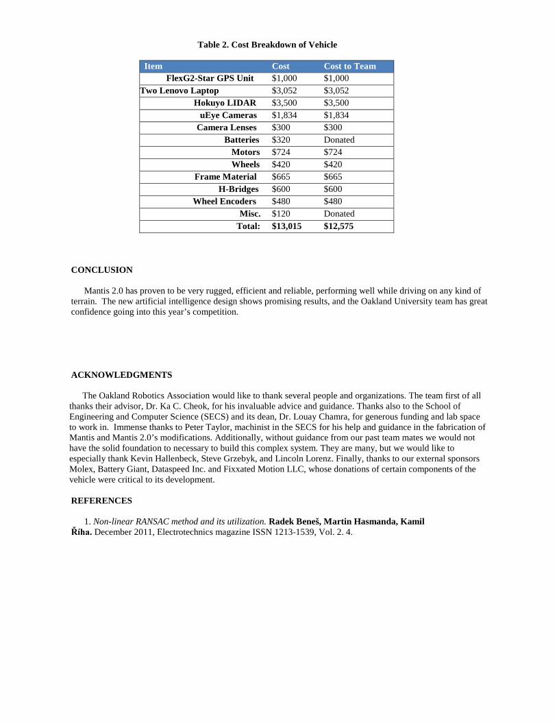
Table 2. Cost Breakdown of Vehicle

Item Cost Cost to Team FlexG2-Star GPS Unit $1,000 $1,000

Two Lenovo Laptop $3,052 $3,052 Hokuyo LIDAR $3,500 $3,500

uEye Cameras $1,834 $1,834 Camera Lenses $300 $300

Batteries $320 Donated Motors $724 $724 Wheels $420 $420

Frame Material $665 $665 H-Bridges $600 $600

Wheel Encoders $480 $480 Misc. $120 Donated

Total: $13,015 $12,575

CONCLUSION

Mantis 2.0 has proven to be very rugged, efficient and reliable, performing well while driving on any kind of

terrain. The new artificial intelligence design shows promising results, and the Oakland University team has great confidence going into this year’s competition.

ACKNOWLEDGMENTS

The Oakland Robotics Association would like to thank several people and organizations. The team first of all

thanks their advisor, Dr. Ka C. Cheok, for his invaluable advice and guidance. Thanks also to the School of Engineering and Computer Science (SECS) and its dean, Dr. Louay Chamra, for generous funding and lab space to work in. Immense thanks to Peter Taylor, machinist in the SECS for his help and guidance in the fabrication of Mantis and Mantis 2.0’s modifications. Additionally, without guidance from our past team mates we would not have the solid foundation to necessary to build this complex system. They are many, but we would like to especially thank Kevin Hallenbeck, Steve Grzebyk, and Lincoln Lorenz. Finally, thanks to our external sponsors Molex, Battery Giant, Dataspeed Inc. and Fixxated Motion LLC, whose donations of certain components of the vehicle were critical to its development. REFERENCES

1. Non-linear RANSAC method and its utilization. Radek Beneš, Martin Hasmanda, Kamil

Říha. December 2011, Electrotechnics magazine ISSN 1213-1539, Vol. 2. 4.