ifrs 17 general measurement model - society of actuaries ......gmm general measurement model (gmm)...
TRANSCRIPT

IFRS 17 –
General Measurement Model
26th April 2019

The views expressed in this presentation are
those of the presenter(s) and not necessarily
of the Society of Actuaries in Ireland
Disclaimer 2
• Introduction
– Previously covered
– TRG updates
– IASB updates
• Overview – Policy Liabilities under IFRS 17
• Present Value of Future Cashflows
• Risk Adjustment
• Contractual Service Margin
• Profit Emergence
• Conclusion
Agenda3
Abbreviations4
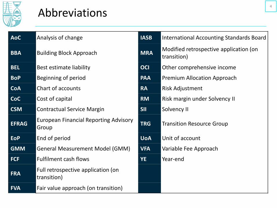
AoC Analysis of change IASB International Accounting Standards Board
BBA Building Block Approach MRAModified retrospective application (on transition)
BEL Best estimate liability OCI Other comprehensive income
BoP Beginning of period PAA Premium Allocation Approach
CoA Chart of accounts RA Risk Adjustment
CoC Cost of capital RM Risk margin under Solvency II
CSM Contractual Service Margin SII Solvency II
EFRAGEuropean Financial Reporting Advisory Group
TRG Transition Resource Group
EoP End of period UoA Unit of account
GMM General Measurement Model (GMM) VFA Variable Fee Approach
FCF Fulfilment cash flows YE Year-end
FRAFull retrospective application (on transition)
FVA Fair value approach (on transition)

Background to the Standard5
IASB’s project on insurance contracts
• IFRS 9 – some insurers will use deferral option until 1 January 2022 based on IFRS 4 amendments
• IFRS 15 is effective 1 January 2018, IFRS 16 is effective 1 January 2019
• Investment contracts without discretionary participation features (e.g. unit linked investments) are in scope of IFRS 9 / IAS 39
• IFRS 17 delayed by a year to 1 January 2022, revised standard due late Q2 2019.
• FASB decided to only make targeted amendments to US GAAP
Insurance project started
1997
Mar2004
IFRS 4 issued
Jan2005
IFRS standards adopted in Europe
Discussion paper
May2007
Jul2010
Exposure Draft of proposals
Jun2013
Exposure Draft of revised proposals May
2017
IFRS 17 issued
Jan2021
OriginalEffective date
Jan2022
RevisedEffective date
June2019
RevisedStandard due

Previously Covered6
• Scope
• Contract classification – IFRS 17 defines insurance contracts as contracts under which significant insurance risk is
transferred.
• Unbundling – distinct components?
• Aggregation – profitable vs onerous contracts, Companies will need to set a definition of ‘similar risks’
and ‘managed together’ and complete a profitability analysis.
• Measurement models – GMM, PAA, VFA.
• Reinsurance – inward (“issued”) vs outward (“held”) reinsurance.
• Transition – Full retrospective, modified retrospective or fair value approach.
• Presentation and disclosures – amounts, judgements and risks.
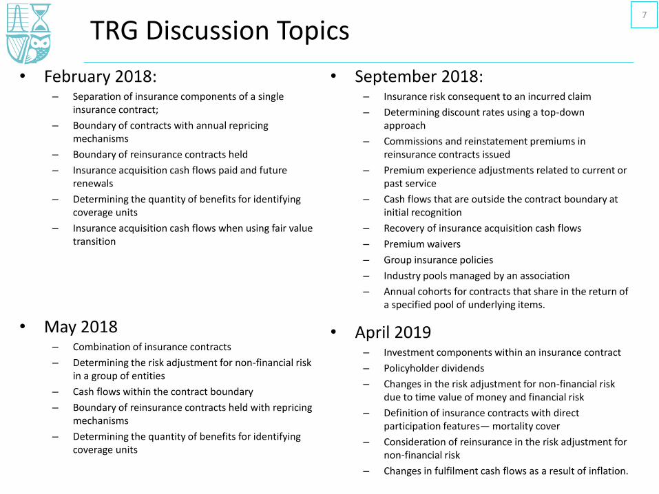
TRG Discussion Topics7
• February 2018:– Separation of insurance components of a single
insurance contract;
– Boundary of contracts with annual repricing mechanisms
– Boundary of reinsurance contracts held
– Insurance acquisition cash flows paid and future renewals
– Determining the quantity of benefits for identifying coverage units
– Insurance acquisition cash flows when using fair value transition
• May 2018– Combination of insurance contracts
– Determining the risk adjustment for non-financial risk in a group of entities
– Cash flows within the contract boundary
– Boundary of reinsurance contracts held with repricing mechanisms
– Determining the quantity of benefits for identifying coverage units
• September 2018:– Insurance risk consequent to an incurred claim
– Determining discount rates using a top-down approach
– Commissions and reinstatement premiums in reinsurance contracts issued
– Premium experience adjustments related to current or past service
– Cash flows that are outside the contract boundary at initial recognition
– Recovery of insurance acquisition cash flows
– Premium waivers
– Group insurance policies
– Industry pools managed by an association
– Annual cohorts for contracts that share in the return of a specified pool of underlying items.
• April 2019– Investment components within an insurance contract
– Policyholder dividends
– Changes in the risk adjustment for non-financial risk due to time value of money and financial risk
– Definition of insurance contracts with direct participation features— mortality cover
– Consideration of reinsurance in the risk adjustment for non-financial risk
– Changes in fulfilment cash flows as a result of inflation.
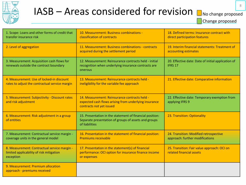
IASB – Areas considered for revision8
1. Scope: Loans and other forms of credit that transfer insurance risk
10. Measurement: Business combinations -classification of contracts
18. Defined terms: Insurance contract with direct participation features
2. Level of aggregation 11. Measurement: Business combinations - contracts acquired during the settlement period
19. Interim financial statements: Treatment of accounting estimates
3. Measurement: Acquisition cash flows for renewals outside the contract boundary
12. Measurement: Reinsurance contracts held - initial recognition when underlying insurance contracts are onerous
20. Effective date: Date of initial application of IFRS 17
4. Measurement: Use of locked-in discount rates to adjust the contractual service margin
13. Measurement: Reinsurance contracts held -ineligibility for the variable fee approach
21. Effective date: Comparative information
5. Measurement: Subjectivity - Discount rates and risk adjustment
14. Measurement: Reinsurance contracts held -expected cash flows arising from underlying insurance contracts not yet issued
22. Effective date: Temporary exemption from applying IFRS 9
6. Measurement: Risk adjustment in a group of entities
15. Presentation in the statement of financial position: Separate presentation of groups of assets and groups of liabilities
23. Transition: Optionality
7. Measurement: Contractual service margin -coverage units in the general model
16. Presentation in the statement of financial position: Premiums receivable
24. Transition: Modified retrospective approach: further modifications
8. Measurement: Contractual service margin -limited applicability of risk mitigation exception
17. Presentation in the statement(s) of financial performance: OCI option for insurance finance income or expenses
25. Transition: Fair value approach: OCI on related financial assets
9. Measurement: Premium allocation approach - premiums received
No change proposed
Change proposed
• Introduction
• Overview – Policy Liabilities under IFRS 17
– Measurement Models - which model when?
– IFRS 17 General Measurement Model
• Present Value of Future Cashflows
• Risk Adjustment
• Contractual Service Margin
• Profit Emergence
• Conclusion
Agenda9
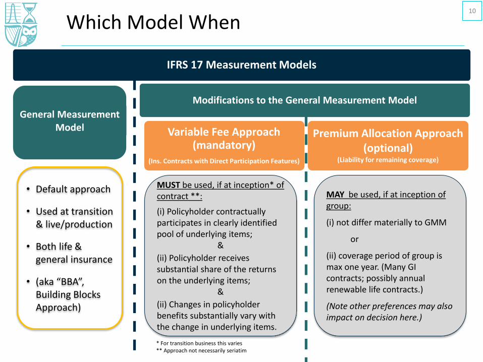
Which Model When
IFRS 17 Measurement Models
General Measurement Model
Modifications to the General Measurement Model
Variable Fee Approach (mandatory)
(Ins. Contracts with Direct Participation Features)
Premium Allocation Approach (optional)
(Liability for remaining coverage)
* For transition business this varies** Approach not necessarily seriatim
MUST be used, if at inception* of contract **:
(i) Policyholder contractually participates in clearly identified pool of underlying items;
&
(ii) Policyholder receives substantial share of the returns on the underlying items;
&
(ii) Changes in policyholder benefits substantially vary with the change in underlying items.
MAY be used, if at inception of group:
(i) not differ materially to GMM
or
(ii) coverage period of group is max one year. (Many GI contracts; possibly annual renewable life contracts.)
(Note other preferences may also impact on decision here.)
• Default approach
• Used at transition & live/production
• Both life & general insurance
• (aka “BBA”, Building Blocks Approach)
10

Which Model When – Likely Product Types
IFRS 17 Measurement Models
General Measurement Model
Modifications to the General Measurement Model
Variable Fee Approach (mandatory)
(Ins. Contracts with Direct Participation Features)
Premium Allocation Approach (optional)
(Liability for remaining coverage)
• Unit linked (UL)
• Variable annuity (VA) & equity index-linked contracts
• Continental European 90/10 contracts
• UK with profits contracts
• Unitised with profits
Judgements re possible breaches of VFA requirements:
• For VA, guarantee aspects.
• For UL, if death benefit sufficient to justify insurance contract treatment.
• European “formulaic with profits”
• Short term general insurance business
• Short term life and certain group contracts
Judgements re possible breaches of PAA requirements:
• For annual renewable business, whether guarantee at renewal date
Long term business
“Life” examples
• Whole of life
• Term assurance
• Protection
• Annuities
• Reinsurance written
“Non-Life” examples
• Multi-year motor
• Warranty cover
• Certain types of Loss Portfolio Transfers / Adverse Development Cover
11
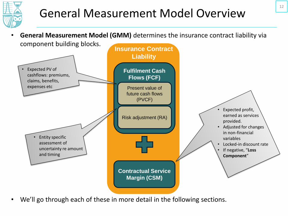
General Measurement Model Overview
• General Measurement Model (GMM) determines the insurance contract liability via component building blocks.
• We’ll go through each of these in more detail in the following sections.
Fulfilment Cash
Flows (FCF)
Contractual Service
Margin (CSM)
Present value of
future cash flows
(PVCF)
Risk adjustment (RA)
Insurance Contract
Liability
• Expected profit, earned as services provided.
• Adjusted for changes in non-financial variables
• Locked-in discount rate• If negative, “Loss
Component”
• Expected PV of cashflows: premiums, claims, benefits, expenses etc
• Entity specific assessment of uncertainty re amount and timing
12

• Introduction
• Overview – Policy Liabilities under IFRS 17
• Present Value of Future Cashflows
– Overview
– Which cashflows?
– Contract Boundaries
– Discount rates
• Risk Adjustment
• Contractual Service Margin
• Profit Emergence
• Conclusion
Agenda13

Present Value of Future Cashflows - Overview
Fulfilment Cash
Flows (FCF)
Contractual Service
Margin (CSM)
Present value of
future cash flows
(PVCF)
Risk adjustment (RA)
Insurance Contract
Liability Expected Future Cashflows:• Based on current estimates• Probability weighted• Unbiased• Stochastic modelling where required for
financial options and guarantees
Time Value of Money• Adjustment to convert the expected future
cashflows into current values
Expected Future Cashflows should:Be within the boundary of the contractRelate directly to the fulfilment of the contractInclude cashflows over which the entity has discretion
14

Examples of cashflows to include:• Claims and benefits paid to policyholders, plus associated costs• Surrender and participating benefits• Cashflows resulting from options and guarantees• Costs of selling, underwriting and initiating that can be directly attributable to a
portfolio level• Transaction-based taxes and levies• Policy administration and maintenance costs• Some overhead-type costs such as claims software, etc.• Adjustment to convert the expected future cashflows into current values
Which Cashflows?
Cashflows excluded:• Investment returns• Payments to and from reinsurers• Cashflows that may arise from future contracts• Acquisition costs not directly related to obtaining the portfolio of contracts• Cashflows arising from abnormal amounts of wasted labour• General overhead• Income tax payments and receipts• Cashflows from unbundled components
15
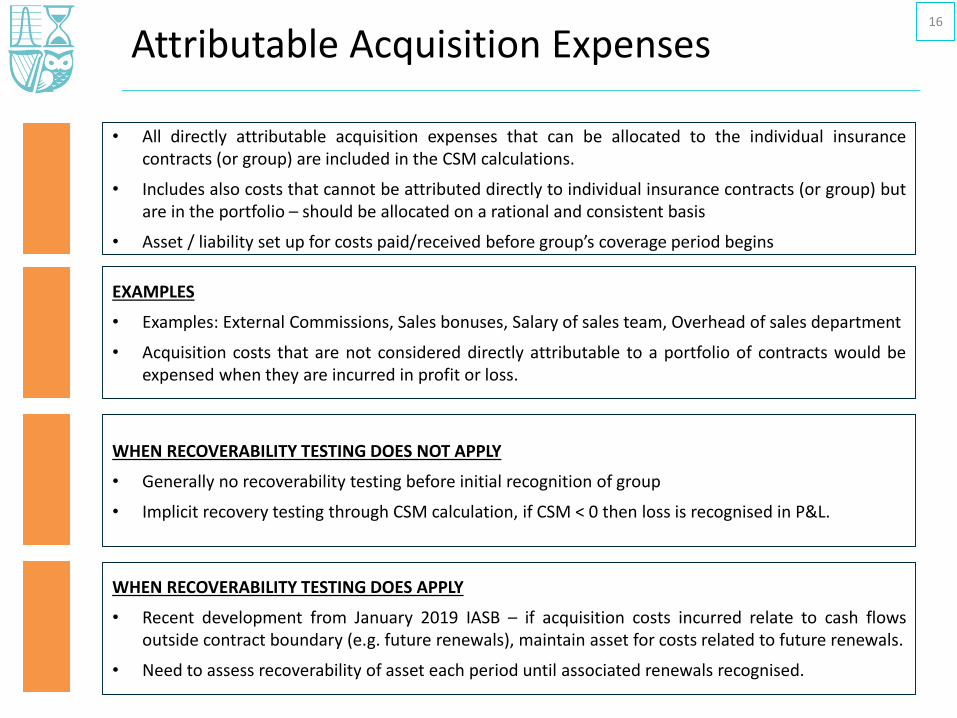
Attributable Acquisition Expenses
• All directly attributable acquisition expenses that can be allocated to the individual insurancecontracts (or group) are included in the CSM calculations.
• Includes also costs that cannot be attributed directly to individual insurance contracts (or group) butare in the portfolio – should be allocated on a rational and consistent basis
• Asset / liability set up for costs paid/received before group’s coverage period begins
WHEN RECOVERABILITY TESTING DOES NOT APPLY
• Generally no recoverability testing before initial recognition of group
• Implicit recovery testing through CSM calculation, if CSM < 0 then loss is recognised in P&L.
WHEN RECOVERABILITY TESTING DOES APPLY
• Recent development from January 2019 IASB – if acquisition costs incurred relate to cash flowsoutside contract boundary (e.g. future renewals), maintain asset for costs related to future renewals.
• Need to assess recoverability of asset each period until associated renewals recognised.
EXAMPLES
• Examples: External Commissions, Sales bonuses, Salary of sales team, Overhead of sales department
• Acquisition costs that are not considered directly attributable to a portfolio of contracts would beexpensed when they are incurred in profit or loss.
16
Contract Boundaries
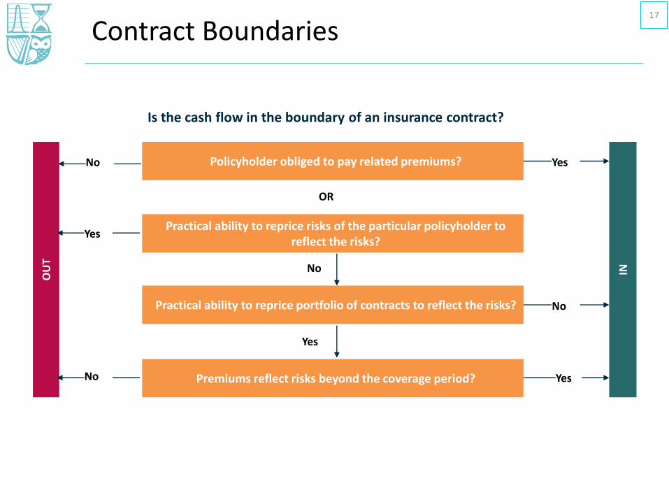
Is the cash flow in the boundary of an insurance contract?
Policyholder obliged to pay related premiums?
OR
IN
Practical ability to reprice risks of the particular policyholder to reflect the risks?
OU
T
Premiums reflect risks beyond the coverage period?
Yes
YesNo
Yes
No
Practical ability to reprice portfolio of contracts to reflect the risks?
Yes
No
No
17
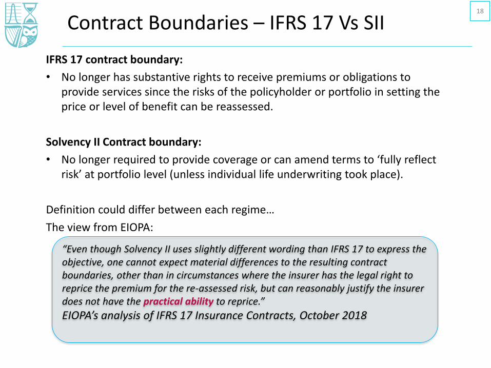
“Even though Solvency II uses slightly different wording than IFRS 17 to express the objective, one cannot expect material differences to the resulting contract boundaries, other than in circumstances where the insurer has the legal right to reprice the premium for the re-assessed risk, but can reasonably justify the insurer does not have the practical ability to reprice.”
EIOPA’s analysis of IFRS 17 Insurance Contracts, October 2018
Contract Boundaries – IFRS 17 Vs SII
IFRS 17 contract boundary:
• No longer has substantive rights to receive premiums or obligations to provide services since the risks of the policyholder or portfolio in setting the price or level of benefit can be reassessed.
Solvency II Contract boundary:
• No longer required to provide coverage or can amend terms to ‘fully reflect risk’ at portfolio level (unless individual life underwriting took place).
Definition could differ between each regime…
The view from EIOPA:
18

Discounting
Market Consistency:
• IFRS 17 requires insurers to use fair value and market-consistent approaches to liability valuations as the basis for reporting their accounts.
• Careful consideration required in constructing the discount rates.
• Two approaches:
– “Top-Down”
– “Bottom-Up”
19

Discounting – “Bottom-Up”
• Foundation is a fully liquid yield curve
• No explicit definition of the basis for deriving a risk free curve
• If using EIOPA what is the UFR?
• Credit Adjustment may be required
• E.g. if underlying instruments carry some level of risk
• Estimating the liquidity adjustment likely to be challenging
• Unlike the Solvency II Volatility Adjustment & Matching Adjustment this must be set by reference to the liabilities rather than the assets.
• Other approaches:
• Bid-ask spreads?
• Pricing hypothetical liquidity swaps?
20
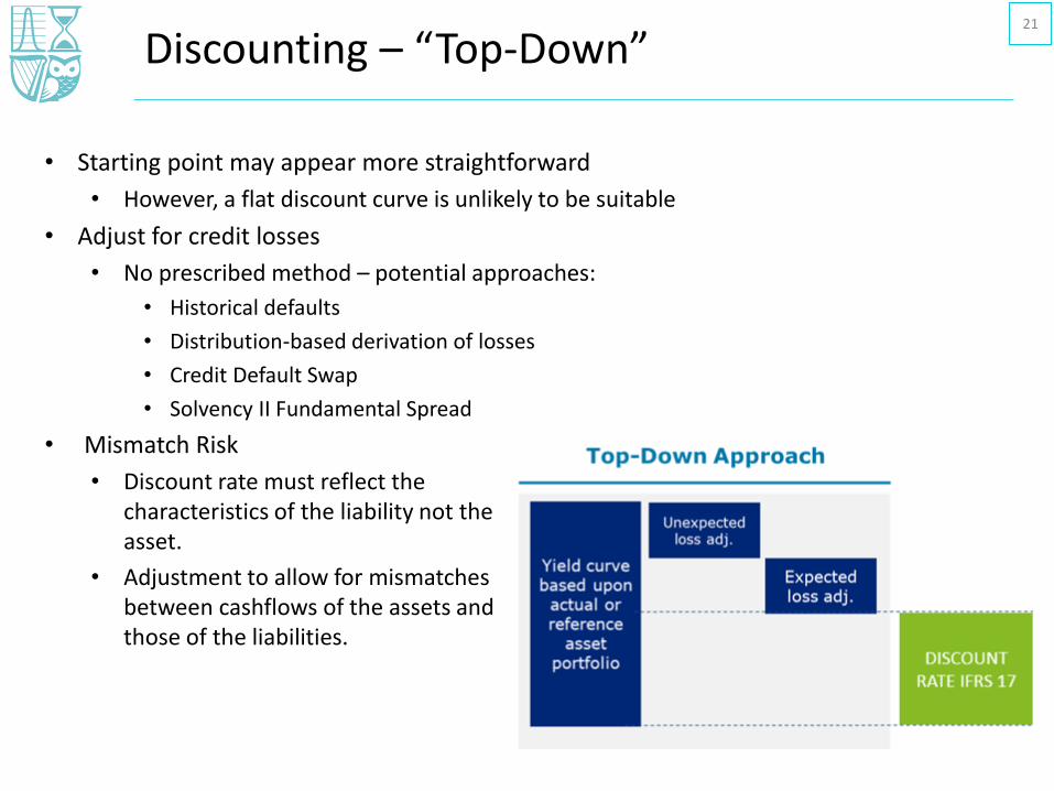
Discounting – “Top-Down”
• Starting point may appear more straightforward
• However, a flat discount curve is unlikely to be suitable
• Adjust for credit losses
• No prescribed method – potential approaches:
• Historical defaults
• Distribution-based derivation of losses
• Credit Default Swap
• Solvency II Fundamental Spread
• Mismatch Risk
• Discount rate must reflect the characteristics of the liability not the asset.
• Adjustment to allow for mismatches between cashflows of the assets and those of the liabilities.
21
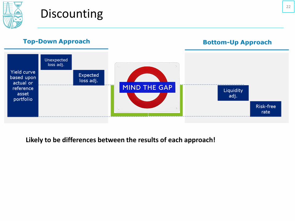
Discounting
Likely to be differences between the results of each approach!
22

• Overview – Policy Liabilities under IFRS 17
• Present Value of Future Cashflows
• Risk Adjustment
– Concept & Background
– Risk Adjustment v Risk Margin
– Risks covered
– Calculation Methods: CoC / VaR / TVaR / PAD
• Contractual Service Margin
• Profit Emergence
Agenda23

Risk Adjustment – Concept
Fulfilment Cash
Flows (FCF)
Contractual Service
Margin (CSM)
Present value of
future cash flows
(PVCF)
Risk adjustment (RA)
Insurance Contract
Liability
The risk adjustment is the compensation that the entity requires for bearing the uncertainty about the amount and timing of the cash flows that arises from non-financial risk.
• Range of possible outcomes versus a fixedcashflow with same NPV are equal
• Entity’s internal view of non-financial risk
24

Risks Covered
Risks Not CoveredRisks Covered
Claim occurrence, amount, timing and development
Lapse, surrender, premium persistency and other policyholder actions
Expense risk associated with costs of servicing the contract
External developments and trends, to the extent that they affect insurance cash flows
Claim and expense inflation risk, excluding direct inflation index linked risk
Financial risk
Asset-liability mismatch risk
Price or credit risk on underlying assets
General operational risk
Risk from cyber attack
25
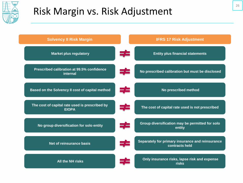
Risk Margin vs. Risk Adjustment
Solvency II Risk Margin
Market plus regulatory
Prescribed calibration at 99.5% confidence
internal
Net of reinsurance basis
Based on the Solvency II cost of capital method
The cost of capital rate used is prescribed by
EIOPA
No group diversification for solo entity
All the NH risks
IFRS 17 Risk Adjustment
Entity plus financial statements
No prescribed calibration but must be disclosed
Separately for primary insurance and reinsurance
contracts held
No prescribed method
The cost of capital rate used is not prescribed
Group diversification may be permitted for solo
entity
Only insurance risks, lapse risk and expense
risks
26
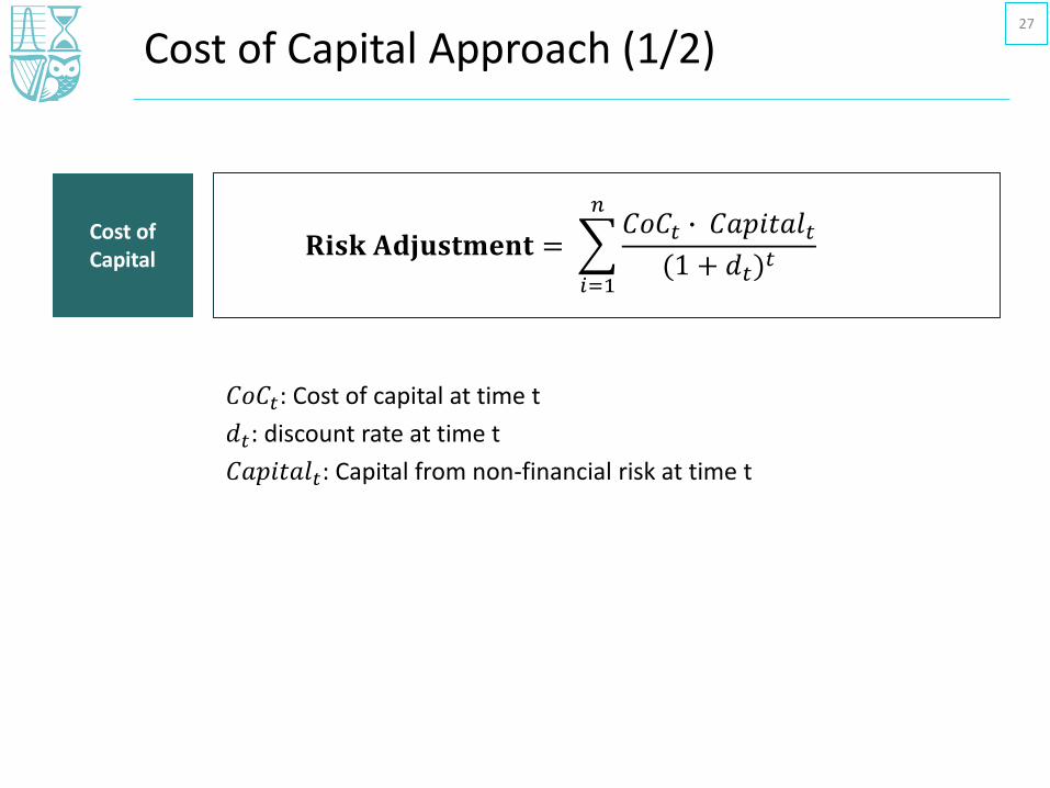
Cost of Capital Approach (1/2)
𝐑𝐢𝐬𝐤 𝐀𝐝𝐣𝐮𝐬𝐭𝐦𝐞𝐧𝐭 =
𝑖=1
𝑛𝐶𝑜𝐶𝑡 ∙ 𝐶𝑎𝑝𝑖𝑡𝑎𝑙𝑡(1 + 𝑑𝑡)
𝑡
27
Cost of Capital
𝐶𝑜𝐶𝑡: Cost of capital at time t
𝑑𝑡: discount rate at time t
𝐶𝑎𝑝𝑖𝑡𝑎𝑙𝑡: Capital from non-financial risk at time t
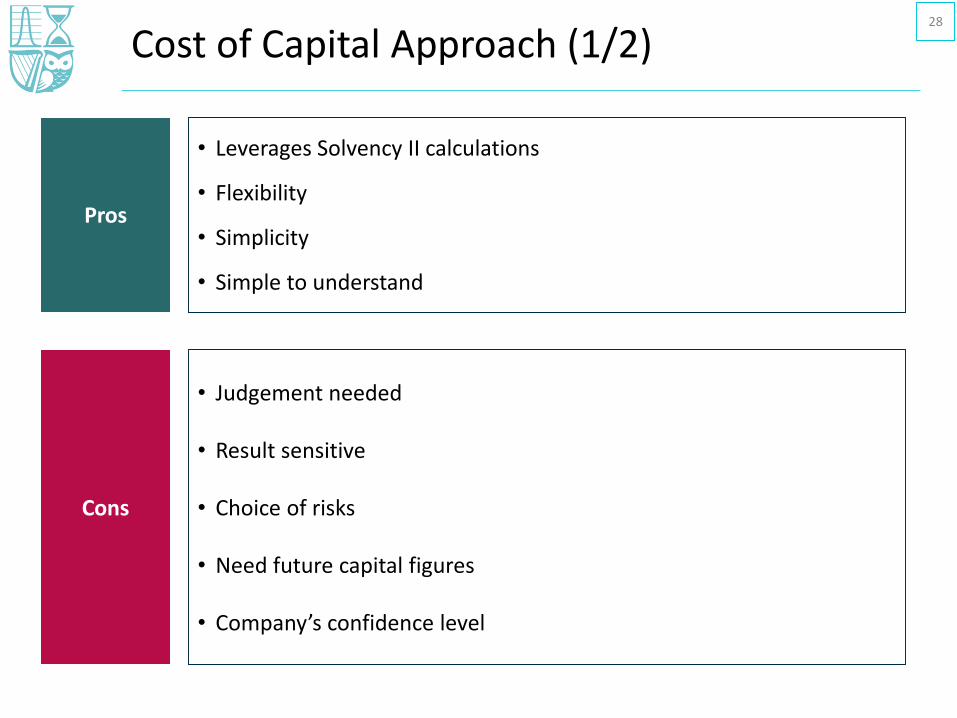
Cost of Capital Approach (1/2)
Pros
• Leverages Solvency II calculations
• Flexibility
• Simplicity
• Simple to understand
Cons
• Judgement needed
• Result sensitive
• Choice of risks
• Need future capital figures
• Company’s confidence level
28
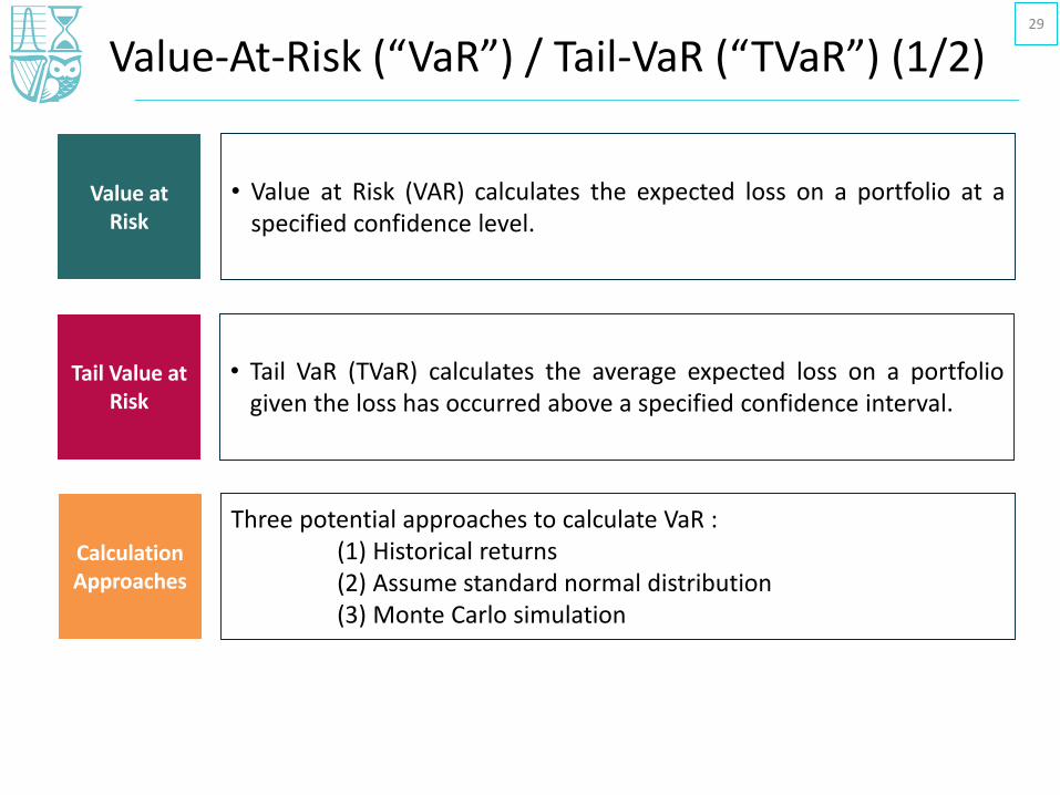
Value-At-Risk (“VaR”) / Tail-VaR (“TVaR”) (1/2)29
Value at Risk
• Value at Risk (VAR) calculates the expected loss on a portfolio at aspecified confidence level.
Tail Value at Risk
• Tail VaR (TVaR) calculates the average expected loss on a portfoliogiven the loss has occurred above a specified confidence interval.
Calculation Approaches
Three potential approaches to calculate VaR :(1) Historical returns(2) Assume standard normal distribution(3) Monte Carlo simulation

VaR / TVaR Approach (2/2)
VaR
• Need to choose confidence interval (for both)
• Easy to communicate (for both)
• Need to calculate the statistical distributions of the liabilities
TVaR
• Highly sensitive in the tail
• Data points in tail may be limited
• Stochastic modelling
30
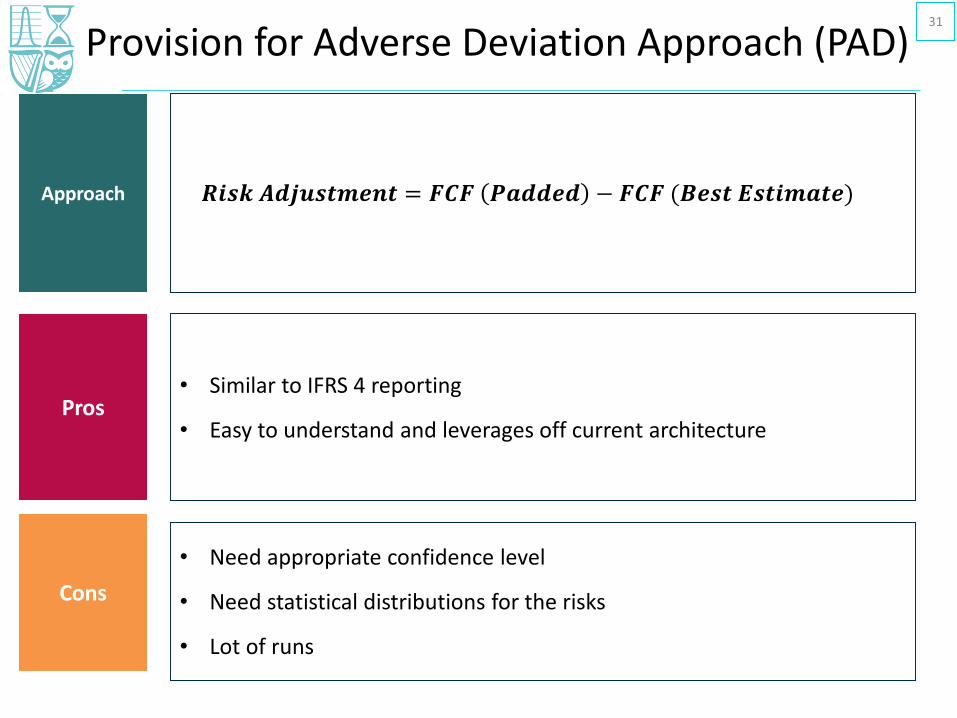
Provision for Adverse Deviation Approach (PAD)
Approach
• Similar to IFRS 4 reporting
• Easy to understand and leverages off current architecture
𝑹𝒊𝒔𝒌 𝑨𝒅𝒋𝒖𝒔𝒕𝒎𝒆𝒏𝒕 = 𝑭𝑪𝑭 𝑷𝒂𝒅𝒅𝒆𝒅 − 𝑭𝑪𝑭 (𝑩𝒆𝒔𝒕 𝑬𝒔𝒕𝒊𝒎𝒂𝒕𝒆)
Pros
Cons
• Need appropriate confidence level
• Need statistical distributions for the risks
• Lot of runs
31

• Introduction
• Overview – Policy Liabilities under IFRS 17
• Present Value of Future Cashflows
• Risk Adjustment
• Contractual Service Margin
– Concept
– Initial Recognition & Subsequent Measurement
– Loss Component
• Profit Emergence
• Conclusion
Agenda32

Contractual Service Margin – Concept
Fulfilment Cash
Flows (FCF)
Contractual Service
Margin (CSM)
Present value of
future cash flows
(PVCF)
Risk adjustment (RA)
Insurance Contract
Liability
New concept under IFRS 17 – profit deferral mechanism measured at a “group” level
• Offsets initial risk adjusted profits (excludingnon-attributable expenses)
• Reduced over time to provide steady release ofprofits into P&L in line with service provided
• Absorbs changes for group profitability relatedto future service (e.g. basis changes)
• Cannot offset losses*, those hit P&L butrecorded and tracked by a Loss Component*Except for Reinsurance Held
Loss Component
33
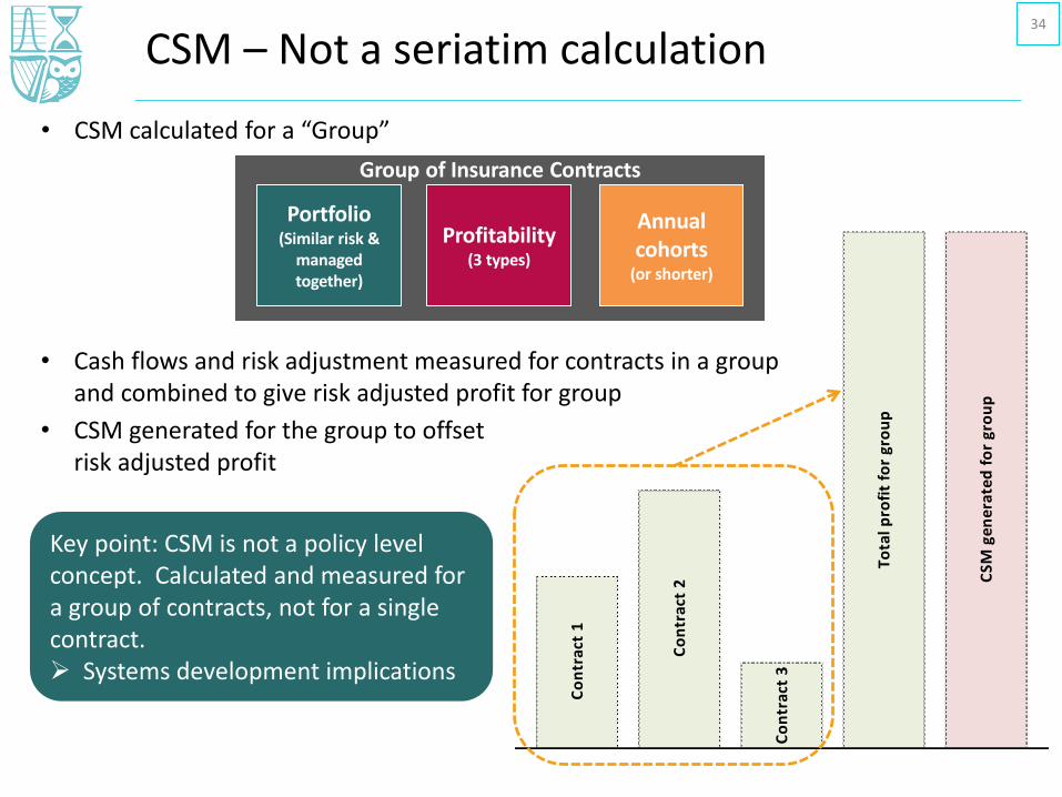
• CSM calculated for a “Group”
CSM – Not a seriatim calculation
• Cash flows and risk adjustment measured for contracts in a group and combined to give risk adjusted profit for group
• CSM generated for the group to offset risk adjusted profit
Co
ntr
act
3
CSM
gen
erat
ed f
or
gro
up
Tota
l pro
fit
for
gro
up
Co
ntr
act
1
Co
ntr
act
2
Key point: CSM is not a policy level concept. Calculated and measured for a group of contracts, not for a single contract. Systems development implications
34
Group of Insurance Contracts
Portfolio(Similar risk &
managed together)
Profitability(3 types)
Annual cohorts
(or shorter)
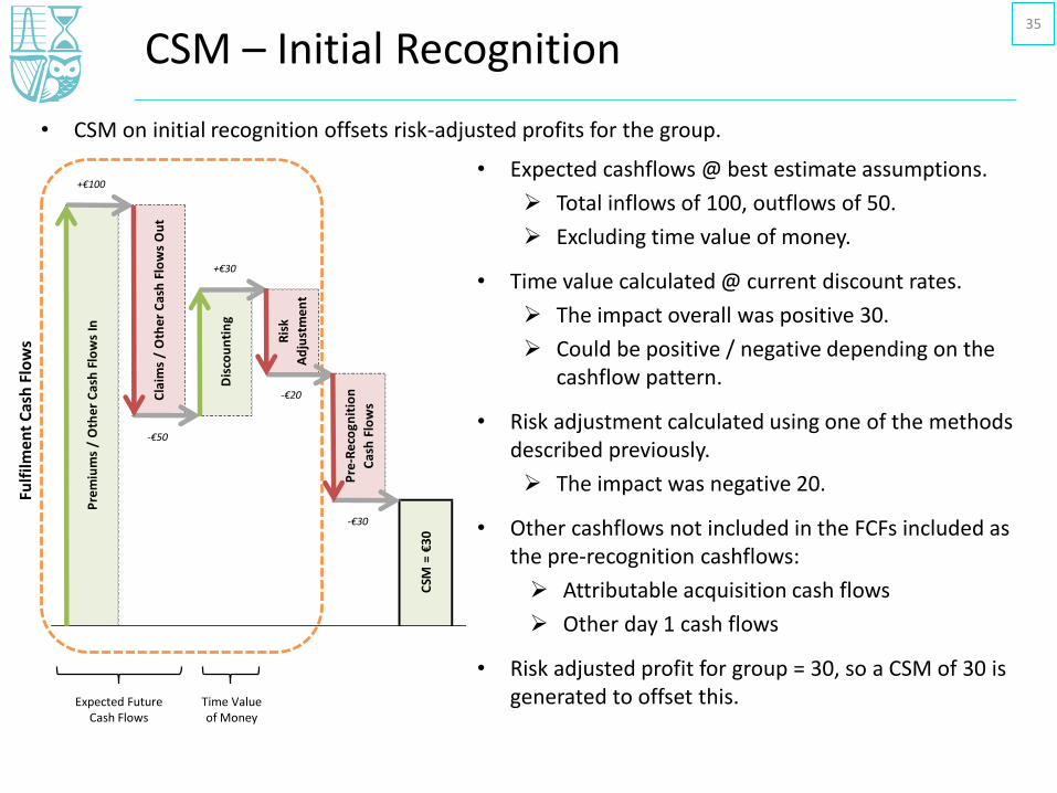
• CSM on initial recognition offsets risk-adjusted profits for the group.
CSM – Initial Recognition
• Expected cashflows @ best estimate assumptions.
Total inflows of 100, outflows of 50.
Excluding time value of money.
• Time value calculated @ current discount rates.
The impact overall was positive 30.
Could be positive / negative depending on the cashflow pattern.
• Risk adjustment calculated using one of the methods described previously.
The impact was negative 20.
• Other cashflows not included in the FCFs included as the pre-recognition cashflows:
Attributable acquisition cash flows
Other day 1 cash flows
• Risk adjusted profit for group = 30, so a CSM of 30 is generated to offset this. Expected Future
Cash FlowsTime Value of Money
Fulf
ilmen
t C
ash
Flo
ws
+€100
+€30
-€20
-€50
-€30
Pre
-Re
cogn
itio
n
Cas
h F
low
s
Ris
k
Ad
just
me
nt
CSM
= €
30
Pre
miu
ms
/ O
the
r C
ash
Flo
ws
In
Cla
ims
/ O
the
r C
ash
Flo
ws
Ou
t
Dis
cou
nti
ng
35

• Graphical illustration of subsequent measurement of CSM over a period.
• Will walk through each step in following slides
CSM – Subsequent Measurement36
Clo
sin
g C
SM
Inte
rest
Acc
reti
on
Ch
ange
s fo
r
Futu
re S
erv
ice
Ne
w B
usi
ne
ss
Fx
Ch
ange
s
Op
en
ing
CSM
Serv
ice
Pro
vid
ed

• The opening CSM balance is the closing CSM balance from the previous reporting period.
CSM – Subsequent Measurement Example37
€60
Op
en
ing
CSM

• The CSM for new business recognised during the period is added.
• This is measured as described previously.
• Only occurs when group is still forming an annual cohort.
CSM – Subsequent Measurement Example38
€30
€60 Ne
w B
usi
ne
ss
Op
en
ing
CSM
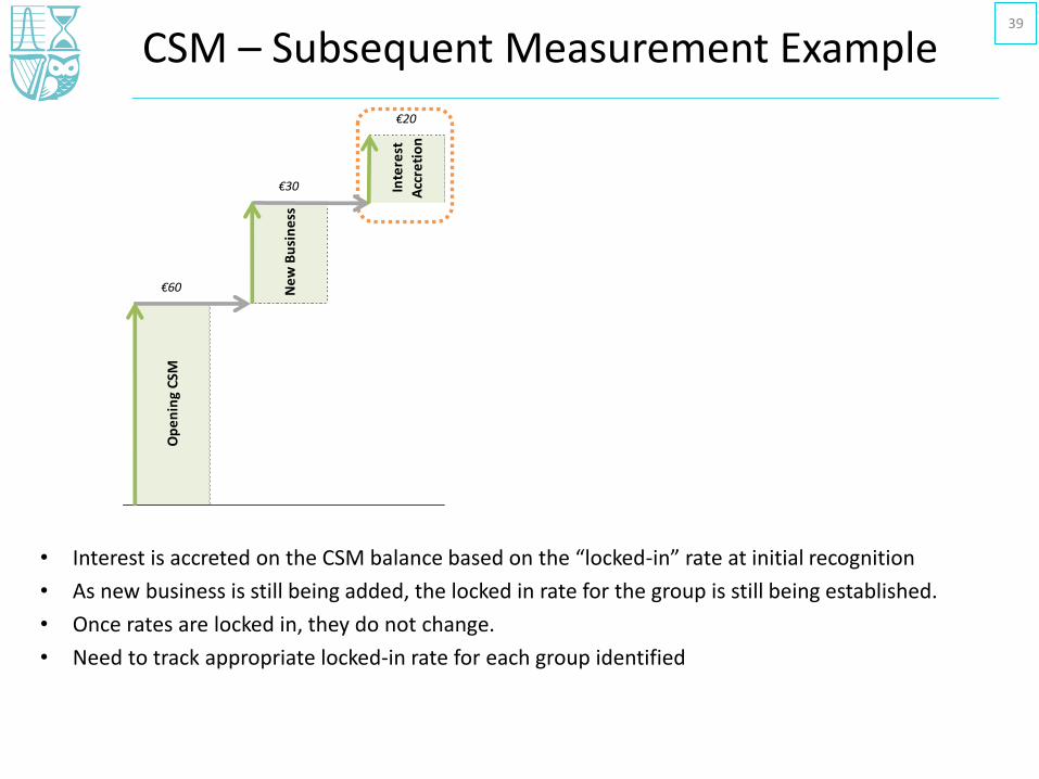
• Interest is accreted on the CSM balance based on the “locked-in” rate at initial recognition
• As new business is still being added, the locked in rate for the group is still being established.
• Once rates are locked in, they do not change.
• Need to track appropriate locked-in rate for each group identified
CSM – Subsequent Measurement Example39
€20
€30
€60
Inte
rest
Acc
reti
on
Ne
w B
usi
ne
ss
Op
en
ing
CSM
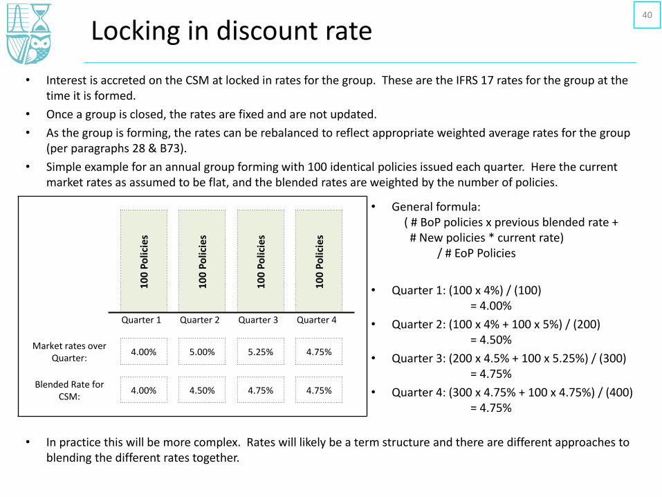
• Interest is accreted on the CSM at locked in rates for the group. These are the IFRS 17 rates for the group at the time it is formed.
• Once a group is closed, the rates are fixed and are not updated.
• As the group is forming, the rates can be rebalanced to reflect appropriate weighted average rates for the group (per paragraphs 28 & B73).
• Simple example for an annual group forming with 100 identical policies issued each quarter. Here the current market rates as assumed to be flat, and the blended rates are weighted by the number of policies.
• In practice this will be more complex. Rates will likely be a term structure and there are different approaches to blending the different rates together.
Locking in discount rate
10
0 P
olic
ies
10
0 P
olic
ies
10
0 P
olic
ies
10
0 P
olic
ies
Quarter 1 Quarter 2 Quarter 3 Quarter 4
Market rates over Quarter:
4.00% 5.00% 5.25% 4.75%
Blended Rate for CSM:
4.00% 4.50% 4.75% 4.75%
• General formula: ( # BoP policies x previous blended rate +# New policies * current rate)
/ # EoP Policies
• Quarter 1: (100 x 4%) / (100)= 4.00%
• Quarter 2: (100 x 4% + 100 x 5%) / (200)= 4.50%
• Quarter 3: (200 x 4.5% + 100 x 5.25%) / (300)= 4.75%
• Quarter 4: (300 x 4.75% + 100 x 4.75%) / (400)= 4.75%
40

• The CSM is adjusted for changes in the fulfilment cashflows that relate to future service
• The impact of these changes is measured at locked in rates – need to value FCFs on locked in rate for CSM.
• Not included here are changes due to financial risk or changes for past/current service
CSM – Subsequent Measurement Example41
Changes include: - Experience Variance for future service- Basis changes for non-financial assumptions
€20
€30
-€30
€60
Inte
rest
Acc
reti
on
Ch
ange
s fo
r
Futu
re S
erv
ice
Ne
w B
usi
ne
ss
Op
en
ing
CSM

• Update for the effect of any currency exchange differences on the CSM
CSM – Subsequent Measurement Example42
€20
€30
-€30
€60
-€20
Inte
rest
Acc
reti
on
Ch
ange
s fo
r
Futu
re S
erv
ice
Ne
w B
usi
ne
ss
Fx
Ch
ange
s
Op
en
ing
CSM
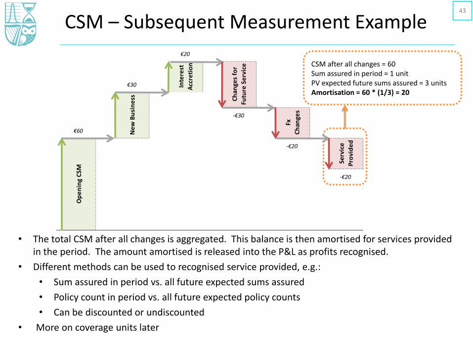
• The total CSM after all changes is aggregated. This balance is then amortised for services provided in the period. The amount amortised is released into the P&L as profits recognised.
• Different methods can be used to recognised service provided, e.g.:
• Sum assured in period vs. all future expected sums assured
• Policy count in period vs. all future expected policy counts
• Can be discounted or undiscounted
• More on coverage units later
CSM – Subsequent Measurement Example
CSM after all changes = 60Sum assured in period = 1 unitPV expected future sums assured = 3 unitsAmortisation = 60 * (1/3) = 20
43
€20
€30
-€30
€60
-€20
-€20In
tere
st
Acc
reti
on
Ch
ange
s fo
r
Futu
re S
erv
ice
Ne
w B
usi
ne
ss
Fx
Ch
ange
s
Op
en
ing
CSM
Serv
ice
Pro
vid
ed
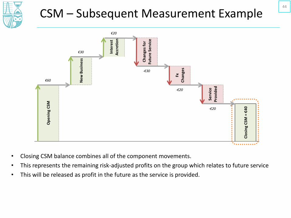
• Closing CSM balance combines all of the component movements.
• This represents the remaining risk-adjusted profits on the group which relates to future service
• This will be released as profit in the future as the service is provided.
CSM – Subsequent Measurement Example
€20
€30
-€30
€60
-€20
-€20
Op
en
ing
CSM
Ne
w B
usi
ne
ss
Serv
ice
Pro
vid
ed
Clo
sin
g C
SM =
€4
0
Inte
rest
Acc
reti
on
Ch
ange
s fo
r
Futu
re S
erv
ice
Fx
Ch
ange
s
44
CSM – Subsequent Measurement Summary
General Measurement Model
Su
bs
eq
uen
t m
easu
rem
en
t o
f C
SM
Opening CSM Balance
New Business
Apply Zero Floor
Comments
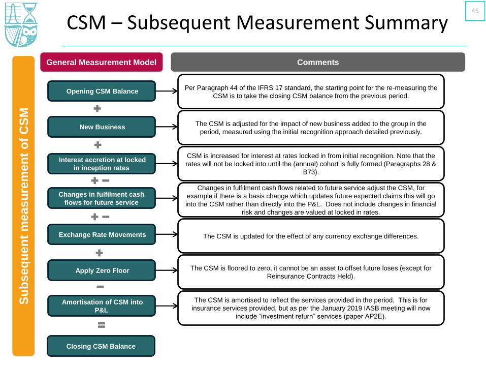
Per Paragraph 44 of the IFRS 17 standard, the starting point for the re-measuring the
CSM is to take the closing CSM balance from the previous period.
The CSM is adjusted for the impact of new business added to the group in the
period, measured using the initial recognition approach detailed previously.
CSM is increased for interest at rates locked in from initial recognition. Note that the
rates will not be locked into until the (annual) cohort is fully formed (Paragraphs 28 &
B73).
Changes in fulfilment cash flows related to future service adjust the CSM, for
example if there is a basis change which updates future expected claims this will go
into the CSM rather than directly into the P&L. Does not include changes in financial
risk and changes are valued at locked in rates.
The CSM is updated for the effect of any currency exchange differences.
The CSM is floored to zero, it cannot be an asset to offset future loses (except for
Reinsurance Contracts Held).
The CSM is amortised to reflect the services provided in the period. This is for
insurance services provided, but as per the January 2019 IASB meeting will now
include “investment return” services (paper AP2E).
Closing CSM Balance
Interest accretion at locked
in inception rates
Changes in fulfilment cash
flows for future service
Exchange Rate Movements
Amortisation of CSM into
P&L
45

• CSM only for deferral of future risk adjusted profits.
• If losses identified, they are immediately recognised in P&L.
• These losses are tracked as a “loss component”. Group can only have a CSM or a Loss Component at any one point in time, but can move between both regularly.
Loss Component
When is Loss
Component generated?
• On initial recognition: Group FCFs + pre-recognition cashflowsare negative. This would likely form an “onerous group”
• On subsequent measurement: Group had CSM, but due toadjustments, e.g. a significant negative basis change, nowviewed as loss making. This could be for an “onerous” or “non-onerous” group.
Important Point: Loss component not necessarily negative equity impact. The risk adjustment also represents unearned profit (compensation for risk) and when released without any adverse experience, may exceed the loss component.
46

€20
€30
€60
-€140
Op
en
ing
CSM
Ch
ange
s fo
r Fu
ture
Se
rvic
e
Loss
Co
mp
on
en
t
= €
30
Inte
rest
Acc
reti
on
Ne
w B
usi
ne
ss
+€70
+€30
-€20
-€50
-€50
Pre
miu
ms
/ O
the
r C
ash
Flo
ws
In
Pre
-Re
cog
nit
ion
Ca
sh F
low
s
Loss
Co
mp
on
en
t
Cla
ims
/ O
the
r C
ash
Flo
ws
Ou
t
Dis
cou
nti
ng
Ris
k
Ad
just
me
nt
Loss Component - Examples
Loss Component on Initial Recognition Loss Component on Subsequent Measurement
Initial recognition: Present value of cash outflows and risk adjustment exceed inflows – the loss amount is recognised in
P&L and loss component established and tracked.
Subsequent measurement: A group here had expected future profits at the start of the period. However a change related to future service had a large negative impact (e.g. basis update)
and eliminated the CSM. The excess hits the P&L and is tracked as a loss component
47
Po
siti
ve B
asis
Ch
ange
= +€
80
CSM
=
€4
0
Loss
Co
mp
on
en
t =
€6
0
Loss
Co
mp
on
en
t =
€5
0
Loss
Co
mp
on
en
t=
€4
0
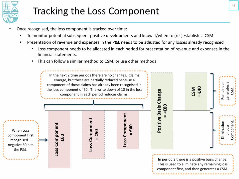
• Once recognised, the loss component is tracked over time:
• To monitor potential subsequent positive developments and know if/when to (re-)establish a CSM
• Presentation of revenue and expenses in the P&L needs to be adjusted for any losses already recognised
• Loss component needs to be allocated in each period for presentation of revenue and expenses in the financial statements.
• This can follow a similar method to CSM, or use other methods
Tracking the Loss Component
When Loss component first
recognised –negative 60 hits
the P&L.
In the next 2 time periods there are no changes. Claims emerge, but these are partially reduced because a
component of those claims has already been recognised in the loss component of 60. The write down of 10 in the loss
component in each period reduces claims.
In period 3 there is a positive basis change. This is used to eliminate any remaining loss component first, and then generates a CSM.
Elim
inat
ion
o
f Lo
ss
Co
mp
on
ent.
Rem
ain
der
ge
ner
ates
a
CSM
.
48
• Introduction
• Overview – Policy Liabilities under IFRS 17
• Present Value of Future Cashflows
• Risk Adjustment
• Contractual Service Margin
• Profit Emergence
– Level of Aggregation Impact
– Coverage Units
• Conclusion
Agenda49
Profit Emergence under IFRS 17
• Profit emergence under IFRS 17 comes from several sources including
• Release of risk adjustment – the “entity’s compensation for accepting risk”
• Release of CSM – the remaining risk-adjusted profit on the portfolio
• Experience variance “noise”
• For CSM, several factors affect profit emergence. The following slides focus on two of those factors:
• The impact of selected level of aggregation
• The selection of appropriate coverage units
50
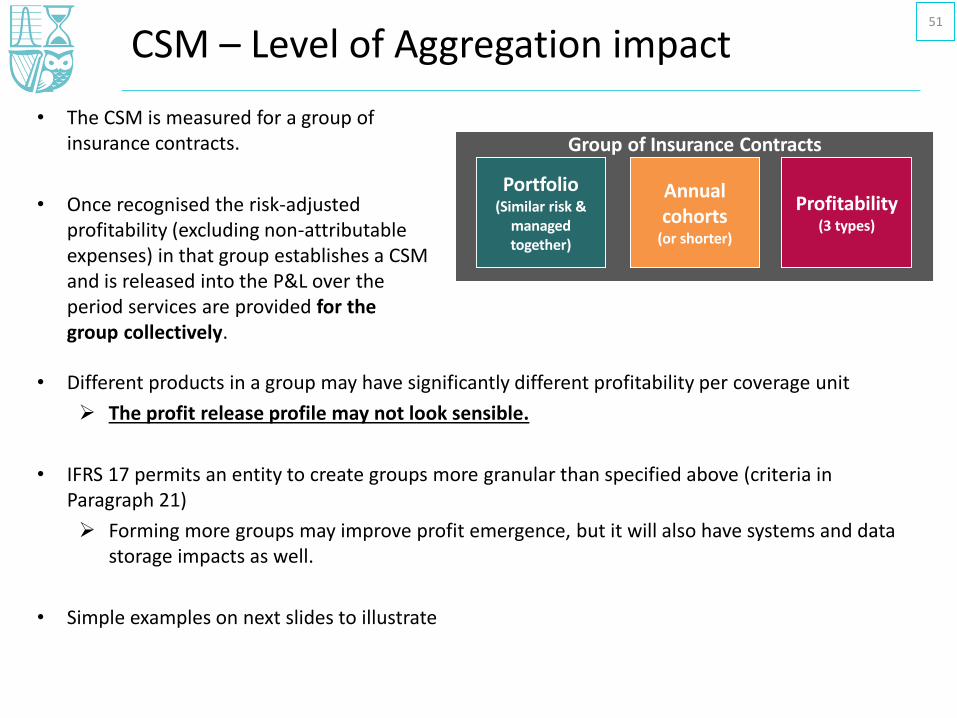
• The CSM is measured for a group of insurance contracts.
• Once recognised the risk-adjusted profitability (excluding non-attributable expenses) in that group establishes a CSM and is released into the P&L over the period services are provided for the group collectively.
CSM – Level of Aggregation impact
Group of Insurance Contracts
Portfolio(Similar risk &
managed together)
Annual cohorts
(or shorter)
Profitability(3 types)
• Different products in a group may have significantly different profitability per coverage unit
The profit release profile may not look sensible.
• IFRS 17 permits an entity to create groups more granular than specified above (criteria in Paragraph 21)
Forming more groups may improve profit emergence, but it will also have systems and data storage impacts as well.
• Simple examples on next slides to illustrate
51

• Simple example: two term products – 5 year and 10 year terms. Both profitable, and same sum assured covered. 5 year product is 3 times more profitable than 10 year product on present value basis.
• This would have the opposite effect if the longer term product were the more profitable – next slide
CSM – Level of Aggregation impact
Ungrouped: Here, the profits from the 5 year product are released over 5 years, and the 10 year product over 10 years.
Grouped: The profits for both products are combined.
• 10 periods of service are provided in the first 5 years (5 periods on each of the two products)
• 5 periods of service are provided in the second 5 years (5 periods for the 10-year product only)
1 2 3 4 5 6 7 8 9 10
P&
L P
rofi
ts
Year
Profitability - Grouped vs. Ungrouped
Ungrouped: 10-year Ungrouped: 5-year Grouped
Important Point: When grouped, some of the profits from the more profitable product are deferred because the profit is viewed as applicable to the entire group as service earned for that group.
52

• Simple example: Same as previous slide, but now 10 year product is 3 times more profitable than 5 year product on a present value basis.
• This is a very simple example, more considerations in practice:
• Complexity of creating additional groups vs. overall impact on profit emergence
• Actual significance of difference in profitability
• Other ways to compensate, e.g. selection of appropriately complex coverage units to recognise service, allowing for discounting in coverage units to reduce impact, etc.
CSM – Level of Aggregation impact
Ungrouped: As before, the profits from the 5 year product are released over 5 years, and the 10 year product over 10 years.
Grouped: As before, profit is identified for the group as a whole. Profitability from different underlying products is ignored & becomes overall profitability of the group. In effect, there is a cross-subsidy between different levels of profitability.
1 2 3 4 5 6 7 8 9 10
P&
L P
rofi
ts
Year
Profitability - Grouped vs. Ungrouped
Ungrouped: 10-year Ungrouped: 5-year Grouped
53
Coverage Units – Introduction
• Recognise profit as it is earned i.e. “spread” CSM over time.
• The CSM amount is allocated equally to each coverage unit.
• How to allocate coverage units consistently?
- Consistency across heterogeneous contracts
- Consistency over time
“Coverage units” establish the amount of the CSM recognised in P&L in the period for a group.
54
CU – Identification & Quantification55
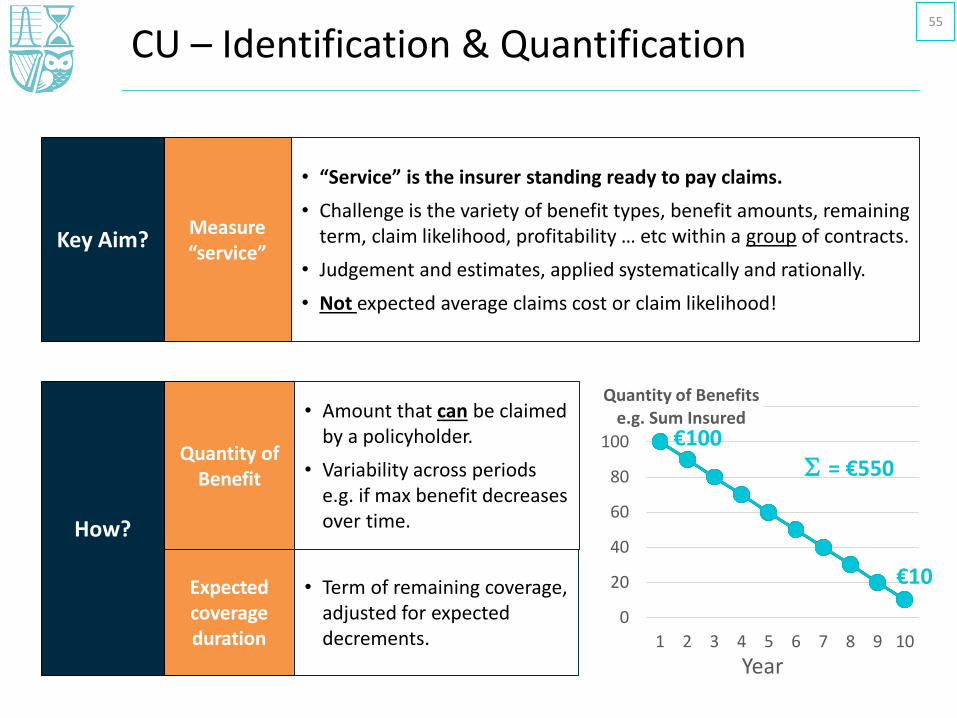
Measure “service”
Key Aim?
• “Service” is the insurer standing ready to pay claims.
• Challenge is the variety of benefit types, benefit amounts, remaining term, claim likelihood, profitability … etc within a group of contracts.
• Judgement and estimates, applied systematically and rationally.
• Not expected average claims cost or claim likelihood!
Quantity of Benefit
How?
• Amount that can be claimed by a policyholder.
• Variability across periods e.g. if max benefit decreases over time.
Expected coverage duration
• Term of remaining coverage, adjusted for expected decrements.
0
20
40
60
80
100
120
1 2 3 4 5 6 7 8 9 10
Quantity of Benefits e.g. Sum Insured
€100
S = €550
Year
€10
CU – Other Considerations
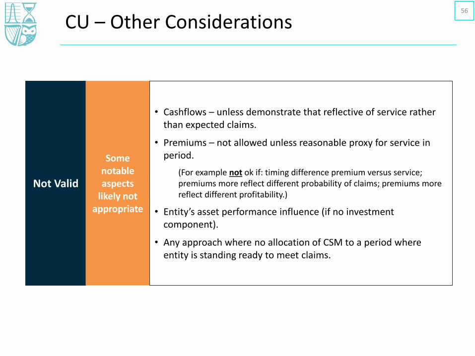
Not Valid
Some notable aspects
likely not appropriate
• Cashflows – unless demonstrate that reflective of service rather than expected claims.
• Premiums – not allowed unless reasonable proxy for service in period.
(For example not ok if: timing difference premium versus service; premiums more reflect different probability of claims; premiums more reflect different profitability.)
• Entity’s asset performance influence (if no investment component).
• Any approach where no allocation of CSM to a period where entity is standing ready to meet claims.
56

CU – Recognition of CSM in P&L
Re-assessment
Ongoing
• At end each period (before any CSM allocation for the period), reassess the expected coverage units and duration.
• Re-allocate CSM equally to each coverage unit (in current period and future periods).
Recognise CSM
P&L• For each period, recognise the amount of CSM (for the group) for
coverage units allocated to that period.
Coverage units relevant
Disclosure
• Explanation of when entity expects to recognise the CSM in the future (either via time bands, or qualitative info)
• General requirement to disclose significant judgements.
57
CU – Simple Example
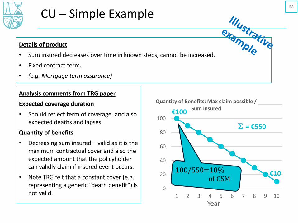
Details of product
• Sum insured decreases over time in known steps, cannot be increased.
• Fixed contract term.
• (e.g. Mortgage term assurance)
Analysis comments from TRG paper
Expected coverage duration
• Should reflect term of coverage, and also expected deaths and lapses.
Quantity of benefits
• Decreasing sum insured – valid as it is the maximum contractual cover and also the expected amount that the policyholder can validly claim if insured event occurs.
• Note TRG felt that a constant cover (e.g. representing a generic “death benefit”) is not valid.
0
20
40
60
80
100
120
1 2 3 4 5 6 7 8 9 10
Quantity of Benefits: Max claim possible / Sum insured
€100
S = €550
€10100/550=18% of CSM
Year
58
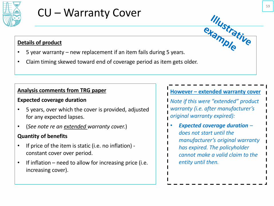
CU – Warranty Cover
Details of product
• 5 year warranty – new replacement if an item fails during 5 years.
• Claim timing skewed toward end of coverage period as item gets older.
Analysis comments from TRG paper
Expected coverage duration
• 5 years, over which the cover is provided, adjusted for any expected lapses.
• (See note re an extended warranty cover.)
Quantity of benefits
• If price of the item is static (i.e. no inflation) -constant cover over period.
• If inflation – need to allow for increasing price (i.e. increasing cover).
However – extended warranty cover
Note if this were “extended” product warranty (i.e. after manufacturer’s original warranty expired):
• Expected coverage duration –does not start until the manufacturer’s original warranty has expired. The policyholder cannot make a valid claim to the entity until then.
59

CU – Health Cover (1/4)
Details of product
Health cover for 10 years, specified types of medical costs.
• Up to €1m total costs covered, over the life of the contract.
• The expected amount and expected number of claims increases with age.
Analysis comments from TRG paper
Expected coverage duration
• 10 years during which cover is provided, adjusted for expected lapse, and any expectations of the limit being reached during the 10 years.
Quantity of benefits
(see next slides, with full details in appendix slide)
60

CU – Health Cover (2/4)
Analysis comments from TRG paper
Quantity of benefits – either:
(a) Constant coverage, max possible claim
• At outset, 10 CU in total, 1 for each year.
• And adjust to reflect claims as they arise (so coverage level reassessed down for all years after a claim, say €0.1m in year 1)
(b) …
1 2 3 4 5 6 7 8 9 10
Quantity of Benefits: Max claim possible
€1m
€0.9m
S = €10m
S = €9.1m
1
10= 10%
of CSM *1
9.1= 10.9%
of CSM ∗∗
Year
Details of product
Health cover for 10 years, specified types of medical costs.
• Up to €1m costs covered, over the life of the contract.
• The expected amount and expected number of claims increases with age.
61
0.9
8.1= 11.1%
of CSM* Year 1, if no claims; ** Year 1 if a 0.1m claim.# Year 2 P&L & Remaining CSM if 0.1m total claims.
#
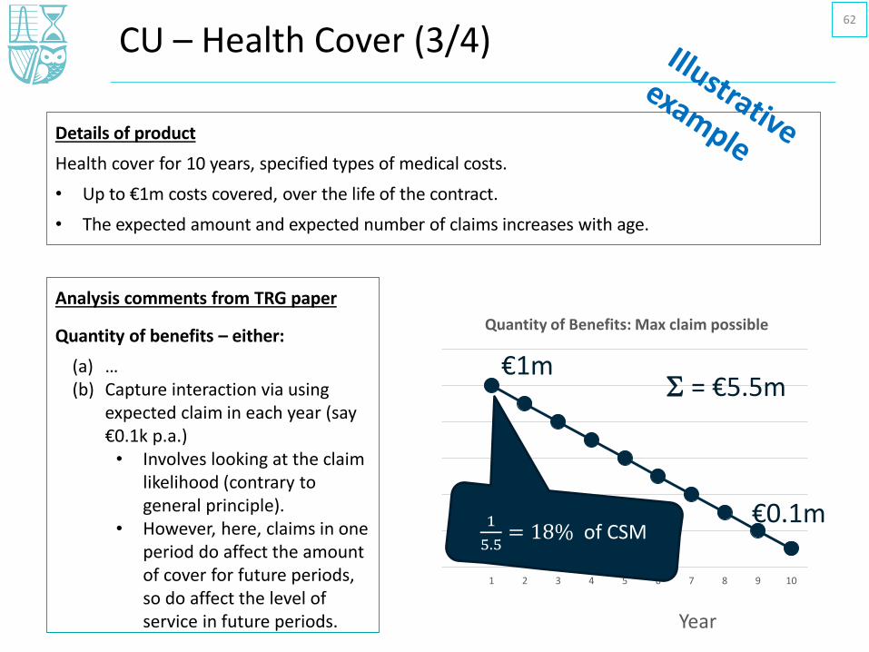
CU – Health Cover (3/4)
Analysis comments from TRG paper
Quantity of benefits – either:
(a) …(b) Capture interaction via using
expected claim in each year (say €0.1k p.a.)
• Involves looking at the claim likelihood (contrary to general principle).
• However, here, claims in one period do affect the amount of cover for future periods, so do affect the level of service in future periods.
1 2 3 4 5 6 7 8 9 10
Quantity of Benefits: Max claim possible
€0.1m
S = €5.5m€1m
1
5.5= 18% of CSM
Year
Details of product
Health cover for 10 years, specified types of medical costs.
• Up to €1m costs covered, over the life of the contract.
• The expected amount and expected number of claims increases with age.
62
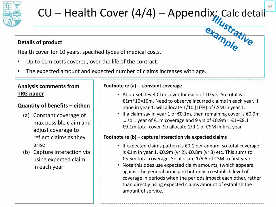
CU – Health Cover (4/4) – Appendix: Calc detail
Analysis comments from TRG paper
Quantity of benefits – either:
(a) Constant coverage of max possible claim and adjust coverage to reflect claims as they arise
(b) Capture interaction via using expected claim in each year
Footnote re (a) – constant coverage
• At outset, level €1m cover for each of 10 yrs. So total is €1m*10=10m. Need to observe incurred claims in each year. If none in year 1, will allocate 1/10 (10%) of CSM in year 1.
• If a claim say in year 1 of €0.1m, then remaining cover is €0.9m … so 1 year of €1m coverage and 9 yrs of €0.9m = €1+€8.1 = €9.1m total cover. So allocate 1/9.1 of CSM in first year.
Footnote re (b) – capture interaction via expected claims
• If expected claims pattern is €0.1 per annum, so total coverage is €1m in year 1, €0.9m (yr 2), €0.8m (yr 3) etc. This sums to €5.5m total coverage. So allocate 1/5.5 of CSM to first year.
• Note this does use expected claim amounts, (which appears against the general principle) but only to establish level of coverage in periods when the periods impact each other, rather than directly using expected claims amount of establish the amount of service.
Details of product
Health cover for 10 years, specified types of medical costs.
• Up to €1m costs covered, over the life of the contract.
• The expected amount and expected number of claims increases with age.
63

CU – Further Examples
Transition Resource Group papers provide several further examples and detailed commentary. (Feb 2018, May 2018)
More complex/bespoke situations are also covered in the TRG examples.
• E.g. unlimited sum insured, unpredictable sum insured, contingent sum insured, multiple benefits on a contract, interactions between benefits on a contract, coverage pattern variations, deferral before coverage, VFA, reinsurance, etc.
Note TRG felt that facts and circumstances are important in forming a valid judgement.
64
• Introduction
• Overview – Policy Liabilities under IFRS 17
• Present Value of Future Cashflows
• Risk Adjustment
• Contractual Service Margin
• Profit Emergence
• Conclusion
Agenda65
Summary – Present Value Future Cashflows66
Cashflows included
• Best estimate future cashflows.
• Relating directly to fulfilment of the contract.
• Within contract boundary.
Contract boundaries
• No longer has substantive rights to receive premiums or obligations to provide services since the risks of the policyholder or portfolio in setting the price or level of benefit can be fully reassessed.
Discounting
• IFRS 17 requires insurers to use fair value and market-consistent approaches to liability valuations as the basis for reporting their accounts.
• Bottom-up or Top-down approach.

Summary – Risk Adjustment67
Cost of Capital
• The Risk Adjustment is calculated as the discounted value of future capital for non-financial risk at required confidence interval multiplied by the company’s internal cost of capital.
Value at Risk
• Value at Risk (VAR) calculates the expected loss on a portfolio at a specified confidence level. This value less the discounted value of best estimate cashflows gives the Risk Adjustment.
Tail Value at Risk
• Tail VaR (TVaR) calculates the average expected loss on a portfolio given the loss has occurred above a specified confidence interval. This value less the discounted value of best estimate cashflows gives the Risk Adjustment.
Provision for Adverse Deviation
• Cashflows revalued using padded non-financial assumptions calibrated to reflect the company’s risks and chosen confidence level. The risk adjustment is the difference between this and the best estimate.

Summary – CSM68
Initial recognition
• At initial recognition, the CSM is set to offset any profits on the group of contracts and represents the unearned profits on that group.
Subsequent Measurement
• Movements will allow for new business, interest accretion, changes in fulfilment cashflows, exchanges rate movements and amortisation.
Loss component
• No negative CSM.
• Losses must be tracked as a loss component.
Profit Emergence
• Level of aggregation effect – CSM is for a group of contracts.
• “Coverage units” establish the amount of the CSM recognised in P&L in the period for a group.

69
Thank you.
Questions?