ific, 6 february 2007 julien lesgourgues (lapth, annecy)
Post on 21-Dec-2015
215 views
TRANSCRIPT

IFIC, 6 FebruaryIFIC, 6 February 2007 2007
Julien Lesgourgues (LAPTHJulien Lesgourgues (LAPTH, Annecy, Annecy))

1) « historical arguments »- flatness problem- horizon problem- monopoles & topological defects
2) basic model- slow rolling scalar field
- primordial fluctuations
3) agreement between CMB maps and inflation- coherence- scale invariance - gaussianity- adiabaticity
4) current constraints on inflation, prospects…
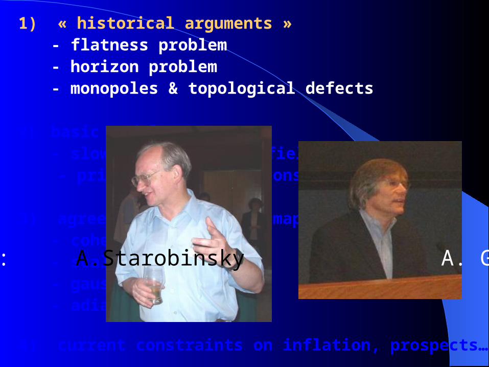
1979-1982: A.Starobinsky A. Guth

1) « historical arguments » : flatness problem
Definitions :
-scale factor : a(t) ds2 = dt2 - a(t)2 dx2 c=1
-e-fold number : N = ln a e.g. “a stage lasts for N=10 e-folds” a(t) increases by factor e10=22000

Friedmann equation :
or :
matter(nr, r)
spatial curvature
a-2 a-3, a-4
1) « historical arguments » : flatness problem
decelerated expansion
H

ln a
ln
matter
radiation
dark energy
?curvature
today
1) « historical arguments » : flatness problem
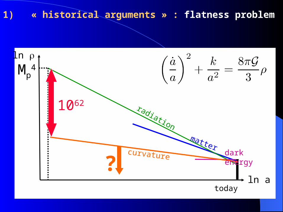
?curvature
Mp4
1062
1) « historical arguments » : flatness problem
ln a
ln
matter
radiation
dark energy
today
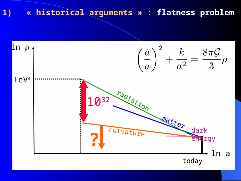
?
TeV4
1032
1) « historical arguments » : flatness problem
curvature
ln a
ln
matter
radiation
dark energy
today

Inflation = stage of accelerated expansion
Friedmann Energy cons. ä(t) > 0 + 3 p < 0
an, -2 < n < 0
1) « historical arguments » : flatness problem

ln a
ln
curvature
matter
radiation
dark energy
today
inflation
1) « historical arguments » : flatness problem

What is the
minimal duration
of inflation ?
1) « historical arguments » : flatness problem
1) « historical arguments » : flatness problem
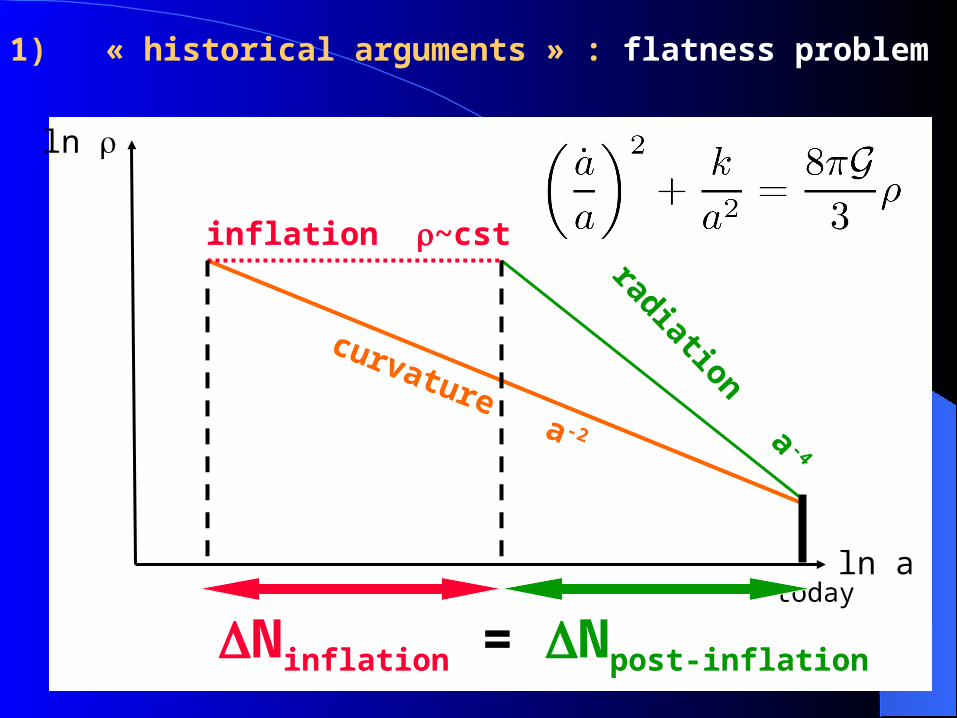
ln a
ln
radiation a -4
today
inflation ~cst
curvature a -2
Ninflation = Npost-inflation

Minimal duration of inflation :
1) « historical arguments » : flatness problem
Ninflation Npost-inflation
transition infl. → rad.
minimal Ninflation
(1016 GeV)4
…(1 TeV)4
~67…
~37
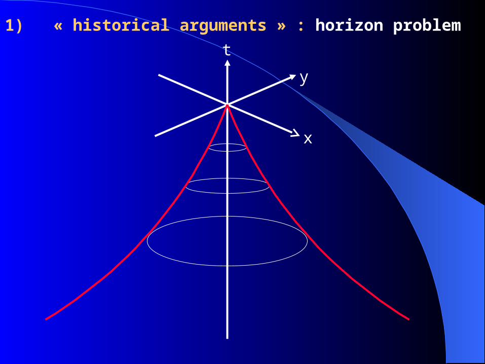
1) « historical arguments » : horizon problem
t
x
y

1) « historical arguments » : horizon problem
t
x
y
last scattering surface (LSS)
are all LSS points within causal contact ?
photondecoupling

1) « historical arguments » : horizon problem
t
x
y
Last scattering surface (LSS)
↓initial singularity
Hubble radius at decoupling: ~1°
photondecoupling

1) « historical arguments » : horizon problem
t
x
y
photondecoupling last scattering surface (LSS)
x
inflation

?curvature
1) « historical arguments » : monopoles and other defects
ln a
ln
matter
radiation
darkenergy
today
phase transition
defects

ln a
ln
curvature
matter
radiation
dark energy
inflation
phase transition
1) « historical arguments » : monopoles and other defects
today

2) Basic model : a slow-rolling scalar field
Inflation = stage of accelerated expansion
Friedmann + e. c. : ä(t) > 0 + 3 p < 0 nearly homogeneous slow-rolling scalar fields :
= ½ ‘2 + V()
p = ½ ‘2 - V()
|dV/d | < V/mP , |d2V/d2|< V/mP2
V

2) Basic model : a slow-rolling scalar field
Inflation = stage of accelerated expansion
Friedmann + e. c. : ä(t) > 0 + 3 p < 0 nearly homogeneous slow-rolling scalar field :
= ½ ‘2 + V()
p = ½ ‘2 - V()
|dV/d | < V/mP , |d2V/d2|< V/mP2
V

2) Basic model : a slow-rolling scalar field
Inflation = stage of accelerated expansion
Friedmann + e. c. : ä(t) > 0 + 3 p < 0 nearly homogeneous slow-rolling scalar field :
= ½ ‘2 + V()
p = ½ ‘2 - V()
|dV/d | < V/mP , |d2V/d2|< V/mP2
V
end of inflation: field oscillates
and decays in particles
which finally thermalize

2) Basic model : primordial cosmological fluctuations
fluctuations today

2) Basic model : primordial cosmological fluctuations
fluctuations at decoupling

2) Basic model : primordial cosmological fluctuations
origin of fluctuations ?

2) Basic model : primordial cosmological fluctuations
decelerated expansion : - causal horizon = Hubble radius ( RH = c/H )
- RH(t) grows faster than a(t)
causal
acausal
timeMATTERDOMINATION
RADIATIONDOMINATION
RHprimodialcosmological perturbations
distance

distance RH
2) Basic model : primordial cosmological fluctuations
phase transition
no coherent fluctuations
decelerated expansion : - causal horizon = Hubble radius ( RH = c/H )
- RH(t) grows faster than a(t)
timeMATTERDOMINATION
RADIATIONDOMINATION
primodialcosmological perturbations

2) Basic model : primordial cosmological fluctuations
RHdistance
INFLATION
accelerated expansion : - causal horizon » Hubble radius
- RH(t) grows more slowly than a(t)
timeMATTERDOMINATION
RADIATIONDOMINATION
primodialcosmological perturbations

2) Basic model : primordial cosmological fluctuations
RHdistance
INFLATION
1
1- quantum fluctuations of and h grow to macroscopic scales- normalization and evolution imposed by quantum mechanics
timeMATTERDOMINATION
RADIATIONDOMINATION
primodialcosmological perturbations

2) Basic model : primordial cosmological fluctuations
RHdistance
INFLATION
1
2- Hubble crossing, Bogolioubov transformation - “squeezed state” → classical stochastic fluctuations
2
timeMATTERDOMINATION
RADIATIONDOMINATION
primodialcosmological perturbations

2) Basic model : primordial cosmological fluctuations
RHdistance
INFLATION
12
3- perturbation amplitude frozen since - «primordial spectrum» of scalar and tensor perturbations
2
3
timeMATTERDOMINATION
RADIATIONDOMINATION
primodialcosmological perturbations

2) Basic model : primordial cosmological fluctuations
RHdistance
INFLATION
12
3
4- insensitive to microscopical evolution (reheating, phase transition)- primordial spectrum mediated to , b, , CDM
4
timeMATTERDOMINATION
RADIATIONDOMINATION
primodialcosmological perturbations

2) Basic model : primordial cosmological fluctuations
RHdistance
INFLATION
12
3
4
5- acoustic oscillations and decoupling- CMB anisotropies → primordial spectrum inherited from 3
5
timeMATTERDOMINATION
RADIATIONDOMINATION
primodialcosmological perturbations

3) Agreement between CMB maps and inflation

inflation predict that perturbations are:
1. coherent
2. nearly gaussian
3. adiabatic*
4. nearly scale invariant*
*for simplest inflationary models
3) Agreement between CMB maps and inflation

RHdistance
INFLATION
decoupling
time coherence of inflationary fluctuations :
3) Agreement between CMB maps and inflation
primodialcosmological perturbations
timeMATTERDOMINATION
RADIATIONDOMINATION

RHdistance
INFLATION
absence of coherence in the case of topological defects :
decoupling
3) Agreement between CMB maps and inflation
primodialcosmological perturbations
timeMATTERDOMINATION
RADIATIONDOMINATION

inflation predict that perturbations are:
1. coherent
2. nearly gaussian
3. adiabatic*
4. nearly scale invariant*
*for simplest inflationary models
3) Agreement between CMB maps and inflation
validated (existence of acoustic
peaks)

inflation predict that perturbations are:
1. coherent
2. nearly gaussian
3. adiabatic*
4. nearly scale invariant*
*for simplest inflationary models
3) Agreement between CMB maps and inflation
validated (statistical analysisof CMB maps)
validated (existence of acoustic
peaks)

inflation predict that perturbations are:
1. coherent
2. nearly gaussian
3. adiabatic*
4. nearly scale invariant*
*for simplest inflationary models
validated (peak scale)
3) Agreement between CMB maps and inflation
validated (statistical analysisof CMB maps)
validated (existence of acoustic
peaks)

inflation predict that perturbations are:
1. coherent
2. nearly gaussian
3. adiabatic*
4. nearly scale invariant*
*for simplest inflationary models
validated (peak scale)
3) Agreement between CMB maps and inflation
validated (statistical analysisof CMB maps)
validated (existence of acoustic
peaks)

slow rolling
scalar field :
AS
kamplitude V3/2/V’
tilt (1-nS) (V’/V)2 , V’’/V
+ hider order corrections
(tilt running, …)
AT
kamplitude V1/2
tilt nT (V’/V)2
+ higher order corrections
(tilt running, …)
V
3) Agreement between CMB maps and inflation
scale invariance :

inflation predict that perturbations are:
1. coherent
2. nearly gaussian
3. adiabatic*
4. nearly scale invariant*
*for simplest inflationary models
validated (peak scale)
3) Agreement between CMB maps and inflation
validated (statistical analysisof CMB maps)
validated (existence of acoustic
peaks)
validated (peak amplitudes)

single field
slow-roll inflation :
AS
kamplitude V3/2/V’
tilt (1-nS) (V’/V)2 , V’’/V
+ next-order corrections
(running of the tilt, …)
AT
kamplitude V1/2
tilt nT (V’/V)2
+ next-order corrections
(running of the tilt, …)
V
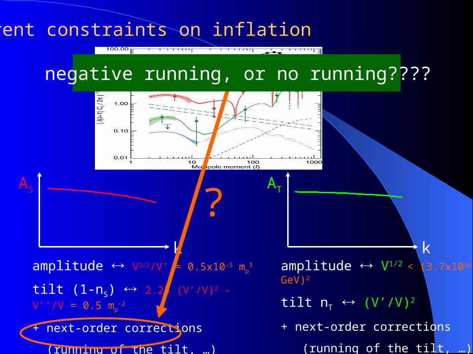
4) current constraints on inflation

AS
kamplitude V3/2/V’
tilt (1-nS) (V’/V)2 , V’’/V
+ next-order corrections
(running of the tilt, …)
AT
kamplitude V1/2
tilt nT (V’/V)2
+ next-order corrections
(running of the tilt, …)
overall amplitude
= 0.5x10⁻⁵ mp3
4) current constraints on inflation

AS
kamplitude V3/2/V’ = 0.5x10⁻⁵ mp
3
tilt (1-nS) 2.25 (V’/V)2 - V’’/V = 0.5
mp-2
+ next-order corrections
(running of the tilt, …)
AT
kamplitude V1/2
tilt nT (V’/V)2
+ next-order corrections
(running of the tilt, …)
overall slope
4) current constraints on inflation

AS
k
AT
kamplitude V1/2 < (3.7x10¹⁶ GeV)2
tilt nT (V’/V)2
+ next-order corrections
(running of the tilt, …)
amplitude V3/2/V’ = 0.5x10⁻⁵ mp3
tilt (1-nS) 2.25 (V’/V)2 - V’’/V = 0.5
mp-2
+ next-order corrections
(running of the tilt, …)
absence of tensors
4) current constraints on inflation

AS
k
AT
kamplitude V1/2 < (3.7x10¹⁶ GeV)2
tilt nT (V’/V)2
+ next-order corrections
(running of the tilt, …)
amplitude V3/2/V’ = 0.5x10⁻⁵ mp3
tilt (1-nS) 2.25 (V’/V)2 - V’’/V = 0.5
mp-2
+ next-order corrections
(running of the tilt, …)
absence of tensors
4) current constraints on inflation
Energy scale of inflation still unknown !!
Self-consistency relation still not checked !!

future CMB experiments (B-polarization) : r ~ 10-2
(factor 50 pour V)
future space-based GW interferometers : r ~ 10-4
(BBO) (factor 5000
pour V)
• measure r, nt : inflationary energy scale + self-consistency r=-8nt
• measure r : inflationary energy scale
• no GW detected : inflation unconstrained
new physics
at 1016 GeV
(extra-D ?)
ordinary QFT
(SUSY, PNGB…)
4) current constraints on inflation
Energy scale of inflation still unknown !!
Self-consistency relation still not checked !!

AS
k
AT
kamplitude V1/2 < (3.7x10¹⁶ GeV)2
tilt nT (V’/V)2
+ next-order corrections
(running of the tilt, …)
amplitude V3/2/V’ = 0.5x10⁻⁵ mp3
tilt (1-nS) 2.25 (V’/V)2 - V’’/V = 0.5
mp-2
+ next-order corrections
(running of the tilt, …)
?
4) current constraints on inflation
AS
k
AT
kamplitude V1/2 < (3.7x10¹⁶ GeV)2
tilt nT (V’/V)2
+ next-order corrections
(running of the tilt, …)
amplitude V3/2/V’ = 0.5x10⁻⁵ mp3
tilt (1-nS) 2.25 (V’/V)2 - V’’/V = 0.5
mp-2
+ next-order corrections
(running of the tilt, …)
?
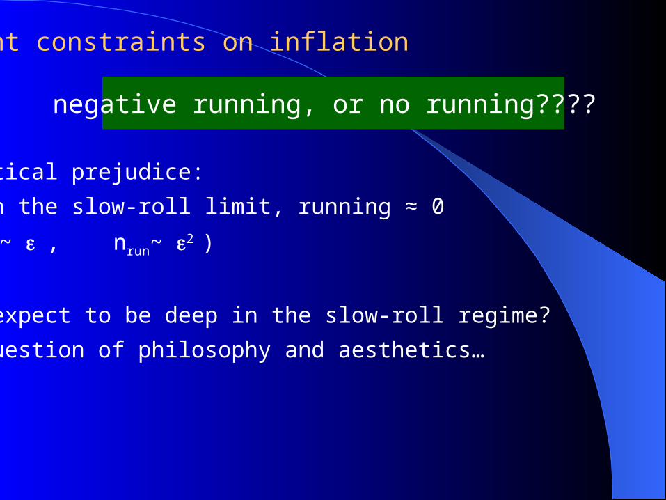
4) current constraints on inflation
negative running, or no running????

4) current constraints on inflation
negative running, or no running????
no running (power law spectrum)
negative running (convex spectrum)
WMAP3+SDSS
4) current constraints on inflation
negative running, or no running????
Theoretical prejudice:
Deep in the slow-roll limit, running ≈ 0
( ns-1 ~ , nrun~ 2 )
Do we expect to be deep in the slow-roll regime?
Question of philosophy and aesthetics…

4) current constraints on inflation
negative running, or no running????
1) Minimalistic aesthetics:
simple potential (monomial, polynomial, simple function)
slow-roll params () monotonically growing/decreasing
60 e-folds before the end, must be deep in slow-roll
expect running ≈ 0
2) Modesty and pragmatism:
V() may have any shape (many scalars, landscape…)
we can only reconstruct “observable region”
(no assumptions on what’s before/after)
possible large running (and beyond)…

4) current constraints on inflation
J.L. & W.Valkenburg, in preparation

0
0.2
0.4
0.6
0.8
r
10.9
Small field models
«mP
CONCAVE, V’’>0
CONVEX, V’’<0
n
large field models
~mP
V3/2/V’ ~ 10-5mp if V’ ~ V/ , V~(1016GeV)4
~mP

0
0.2
0.4
0.6
0.8
r
10.9
CONCAVE, V’’>0
CONVEX, V’’<0
=6
=4
=2
monomial potentials V=(...)
=1
n

0
0.2
0.4
0.6
0.8
r
10.9
CONCAVE, V’’>0
CONVEX, V’’<0
=6
=4
=2
new inflationV=V0 [1- (…) +...]
=1
monomial potentials V=(...)
n

0
0.2
0.4
0.6
0.8
r
10.9
CONCAVE, V’’>0
CONVEX, V’’<0
=6
=4
=2
monomial
=1
Loop correction
monomial potentials V=(...)
Hybrid inflation
=1new inflation
V=V0 [1- (…) +...]
n

0
0.2
0.4
0.6
0.8
r
n 10.9
CONCAVE, V’’>0
CONVEX, V’’<0
=4
=2
monomial
=1
Loop correction
monomial potentials V=(...)
new inflationV=V0 [1- (…) +...]
=1
=6
WMAP-3
WMAP-3+SDSS