if i had this to do over | a twelve step program to successfully
TRANSCRIPT

If I Had This To Do Over….. A Twelve Step Program to Successfully Measure Sewer Rehabilitation
Patrick. L. Stevens*, P.E., ADS Environmental Services, 1300 Meridian Street, Suite 300, Huntsville, AL 35801 [email protected] Peter N. Keefe, ADS Environmental Services, 7421 Sherwood Drive, Mentor, OH 44060 ABSTRACT It has often been said that the best way to learn how to do a thing is to ask experienced people what mistakes they have made and what corrective steps they took in subsequent projects. The goal of this paper is to relay the top twelve issues in the sewer evaluation and rehabilitation process that the authors have identified by asking that question to themselves and others who have experienced both success and failure about their biggest mistakes and greatest triumphs in the measurement of effectiveness of sewer rehabilitation. The sewer rehabilitation ‘industry’ has a long history of falling short of expected Infiltration Inflow (I/I) reduction. In the mid-1980s, the EPA Construction Grants Program would not award a grant to an applicant predicting that more than 30%of RDII will be removed from a collection system through rehabilitation. This limitation was established in the belief that higher removal rates were not possible. A grant applicant sizing a plant based on 60% RDII removal will end up with an undersized WWTP if only 30% is removed. Many practitioners assume the ineffectiveness lies in the rehabilitation technology used, the extent of rehabilitation or sources of I/I in private sewers that went unaddressed. While the rehabilitation work may contribute to the problem, it is evident to the authors that the approach to measuring I/I removal may contribute as much to the apparent ineffectiveness as the work itself. WERF Project 99-WWF-8 studied I/I removal programs around the US and found that their efforts to acquire detailed analysis were unsuccessful for many utilities because information was not generated and archived suitably or that the data were incomplete or unreliable. The mismatch of methods and procedures for evaluating I/I created a lack of uniformity among agencies performing the sewer rehabilitation. The paper will contain specific recommendations and graphic examples of successful and unsuccessful practices for the measurement of RDII effectiveness. This paper is intended to be useful to both the first-time and experienced I/I project managers who are establishing capital improvement programs for sewer rehabilitation and want to be able to answer the future question – “What have you accomplished with the money?” KEYWORDS: Infiltration/Inflow, I/I, Rainfall Dependent I/I, RDII, Forensic RDII Analysis, Q vs. i plots, scattergraphs, Potential I/I, Sliicer.com, Sewer Rehabilitation Measurement, Basin Size, 10/20 Rule

DISCUSSION
After 35 years of performing Infiltration Inflow studies and conducting ‘Forensic RDII’ analyses of sewer rehabilitation work, the authors developed a twelve step program or check list of items that will assure that I/I measurements needed to evaluate sewer rehabilitation are valid and are useful. Much of the information on this list comes from I/I practitioners from around the country who have completed this statement; ‘If I had this to do over, I would _________________’. Some of the information is the result of ‘Forensic RDII Analysis’ which is an audit of flow and rain data for several before- and after-rehabilitation projects. The effectiveness of sewer rehabilitation projects can be derailed early, easily and often. Many derailments occur early in the process and seem totally unrelated to the final outcome, yet are often unrecoverable. It is only after rehabilitation is complete that many communities realize that they do not have enough data or the right kind of data to measure success or failure. Similarly, many rehabilitation projects seem to work very well until a heavy storm comes along and the sewers overflow yet again into basements and streams. Many sewer rehabilitation projects require an engineering evaluation to document the degree of RDII reduction. Often the conclusion contains exculpatory language such as this actual paragraph from such a report;
“Due to the inequality of the conditions in Post-rehab flow monitoring versus Pre-rehab flow monitoring …..the magnitude of improvements made to the collection system can not be measured. Given equal antecedent conditions in Post-rehab versus Pre-rehab significant improvements will be clearly evident. Therefore, this comparison does not show the totality of the improvements made to the collection system”. Citation not given to protect the uninformed and unsuccessful.
The authors believe there are essentially three fates for sewer rehabilitation projects as shown in Figure 1. From left to right the three fates are: A) RDII is reduced and there are clear and measurable results, B) There are subjective reasons to believe RDII may have been removed, but it cannot be quantified and C) There was no apparent reduction of RDII with symptoms remaining unchanged or worse. The purpose of this paper is to address those projects that fall into category ‘B’. Projects falling into this category would have been in category ‘A’ except for an adequate plan for
Fate of Sewer Rehabilitation Projects
Sewer Rehabilitation
Projects
A.RDII Reduced
Everyone HappyPromotion
C.No Apparent Reduction
SSOs & BasementFlooding Continue
B.RDII Reduced
But Can’t Demonstrate or Quantify
Followed No RecipeDid Not Address Private SourcesPiecemeal RepairRely on Smoke Testing OnlyRely on TV onlyRepaired only ManholesRepaired only MainlinesNo Initial Flow MeasurementUse Poor Rehab TechnologyUpstream Restricted Sewer
‘Toilet Paper is Not as High in the Trees as it Used to be’
Do Not Try to Measure
Forensic RDII RevealsTwelve Stumbling Blocks
Followed RecipePlan for Post-rehabExtremely Lucky
Figure 1 The Three Fates of Sewer Rehabilitation Projects

demonstrating a reduction in RDII. In many ways these projects conform to the adage that ‘you can’t manage what you don’t measure’. It is believed that projects end up in the ‘C” category for several reasons. Shortcomings in the actual implementation of the work may contribute to the problem, including an inadequate job of locating the sources of RDII, piecemeal repair of sewers with no plan for migration, repairing only public sewers and many others. Similarly, projects may end up in the ‘C’ category because they failed in the up front diagnostic work needed to locate and quantify sources or areas of excessive RDII. This list of 12 items also is a recipe for developing a suitable diagnostic effort. Top Twelve Hydrologic Reasons for Poor Rehab Results.
1. Rain gauge Strategy - This includes the density of the RG network and where the RGs are placed.
2. Duration - Not enough data (dry days and storms of differing magnitudes) to generate proper and statistically valid rain-to-flow relationships (Q vs. i).
3. Key Performance Indicators – Scattergraphs and Q vs. i diagrams.
4. Flow Meter Depth Technology.
5. Size of Meter Basins.
6. Seasons for Measurement.
7. Rainfall Data Frequency.
8. Pain of Subtraction.
9. Faulty Method of Calculating RDII.
10. Dynamics of sewers (restricted) and “Potential I/I” (Q vs. i is flat).
11. Lack of Control Basin.
12. Site Hydraulics at Metering Sewer.

1. Rain Gauge Strategy
Rainfall issues are at the top of the list because inadequate rainfall data is the most common stumbling block to proper measurement of RDII. People often think of an RDII study primarily as a flow metering effort and the collection of rainfall data is often an ‘after thought’. It is not uncommon for an Agency’s scope of work to describe in great detail the type of flow metering technology, the field services expected and the level of data processing expected, yet specifies just a few rain gauges or even relies on existing sources of rain data from the airport or the water treatment plant. What is missing in this approach is the awareness that in the relationship between rainfall and RDII, rainfall data are mathematically just as important as flow data. “It’s the rainfall stupid.” Some people use ‘rules of thumb’ for rain gauge placement that are based on the number of flow meters used, e.g. add one rain gauge for every 10 (or so) flow meters. This approach may result in an adequate number of rain gauges if sewer sheds are small, but in large sewer sheds, this approach will result in too few rain gauges. For small studies the use of a meter-to-rain gauge ratio will often result in a single rain gauge being placed. Rain gauges should be treated the same way we treat pumps in pump station designs. We always assume one will fail so at least two are deployed. Similarly a flow study should never have less than two rain gauges. Agencies new to RDII measurement seem to be unaware of how primitive a tipping bucket rain gauge is and that it is relatively easy to become plugged. It is the author’s experience that an uptime of 80% for a permanently-installed rain gauge network is a high value. Rain gauge density is a second issue that is often overlooked and many agencies view rain gauges as nothing more than an expense that needs to be minimized. In March 2011 Water Underground Infrastructure Management (UIM 2011) conducted a Webinar on the topic of this paper. The registration process asked participants to answer a few questions and one question was on the importance of accurate flow and rain measurement in quantifying RDII. Figure 2 shows the results of the survey question on the importance of accurate flow and rain data. Over half the respondents believed that rainfall data from any nearby facility was adequate. Recommendations for the density of rain gauges for urban hydrology vary considerable. Three published references recommend rain gauge densities and they are listed below. There is a ten-fold difference in the recommendations for rain gauge density.
Existing Sewer Evaluation and Rehabilitation, 3rd Edition by WEF/ASCE recommends “one rain gauge for every 5 to 10 square miles, subject to a minimum of two gauges – even for small projects.”
How important are accurate flow and rain measurement in quantifying RDII?
4%
57%
39%
a) Not important – a ‘rough’ ideais sufficient for my work
b) Flow data are important, butany rain data from any nearbyfacility will work.
c) Mathematically flow and raindata have equal significance inquantifying RDII.
Figure 2 Results of UIM Webinar Questionaire.

Code of Practice for the Hydraulic Modeling of Sewer Systems, Version 3.001, November 2002 by the Wastewater Planning Users Group (WaPUG) recommends the following:
Flat Terrain: 1 + 1 per 4 km2 (1 + 1 per 1.5 mi2) Average: 1 + 1 per 2 km2 (1 + 1 per 0.8 mi2) Mountainous: 1 + 1 per 1 km2 (1 + 1 per 0.4 mi2)
Water Research Centre (1987). A Guide to Short Term Flow Surveys of Sewer Systems, WRc
Engineering, Wiltshire, England.
Same as the WaPUG recommendation above. It appears this document is the original source of recommendations used in the above WaPUG 2002 document. However, the WRc document does not reference any of its sources.
Radar Rainfall service providers can deliver rainfall information at a 1 km2 resolution and generally want to see a network of calibrating rain gauges at a density of one gauge per 10 mi2. With such a wide range of recommended rain gauge densities, how is the manager to decide on a density for the Agency’s flow metering project? The selection depends on whether you ever expect to answer the question ‘What have you accomplished with the money?’ Remember that in the rain-to-flow relationship, rainfall is the independent (and most important) variable and RDII is the dependent variable. A person who is planning a rain gauge network for RDII work can convince themselves of the importance of a dense rain gauge network by studying rainfall patterns as measured (estimated) by NEXRAD radar. The reader can find the local radar from this National Weather Service web page. http://www.weather.gov/radar_tab.php Figure 3 is screen capture from the Nashville NEXRAD showing a single reflectivity image for a single scan and it appears that this storm will produce plenty of rainfall for RDII measurement. One of the NEXRAD products shows the estimated storm total rainfall and the last hour’s accumulated rainfall.
Figure 3 A snapshot of the NEXRAD Base Reflectivity of the Nashville, TN radar.

Figure 4 shows the last hour accumulation. The reader will find that the more intense the rainfall, the smaller the foot print of the rain. The bubble text in Figure 4 show points to a band of green rainfall. The green footprint of rainfall exceeding 0.5 inches is just 6 miles wide and the footprint of rainfall of 1.2 inches (yellow) is just 0.6 miles (1 km) wide. Imagine that an agency is conducting an RDII study or calibrating a model in a sewershed in this rainfall footprint. Depending on the rain gauge density the measured rainfall could have been 0.5 or 1.2 inches for the hour. This can make a huge difference in model calibration or RDII measurement.
The green band (>1/2 inch) is 6 miles wide the yellow cells (1.2 inches)
is 0.6 miles wide
Figure 4 The rainfall footprint for the preceding hour. The observation is that more intense rainfall occurs in narrower footprints.

For RDII measurement in large areas the rain gauges should be laid out in a grid so that a storm with a narrow footprint can’t sneak through undetected. For small areas, the placement of a rain gauge in each sewer shed may be acceptable, but make sure the gauges are no farther that ~ 2 miles apart. Rainfall can be calculated for each sewer shed through some distribution algorithm. Common algorithms include Closest Rain Gauge, Theissen Polygon, Inverse Distance and Inverse Distance Squared. Summary recommendations from the authors for a rain gauge strategy are:
Never less than two (always assume that one will fail) 1-2 Mi2/RG in convective storm season or in hilly areas 2-4 Mi2/RG in cyclonic/frontal storm season Rain gauges should be placed on a grid, not necessarily in each basin Don’t rely on distant rain gauges such as from an airport
4 Miles
T=0 Min.
T=30 Min.
4 Miles
T=0 Min.
T=30 Min.
Figure 5 Rain gauges should be laid out in a grid pattern.

2. Duration of Measurement
It is often said that the best way to bring about a drought is to install flow meters in sewers. While this is sometimes true, it is also true that many projects suffer from insufficient dry-weather data. Dry weather data are needed to determine the Waste Water Production and Base Infiltration in a sewershed. In an attempt to assure that an RDII project experiences sufficient rainfall Agencies will schedule the work for the historical ‘wet’ period for the area. However this strategy can backfire if the season is wetter than normal and if there are no dry days. In March 2011 Water Underground Infrastructure Management (UIM 2011) conducted a Webinar on the topic of this paper. The registration process asked participants to answer a few questions and one question was on the proper duration of flow measurement for RDII studies. Figure 6 displays the results of the survey and most respondents believe a dry and wet period were appropriate. The views about the proper duration of an RDII study have changed over the last 20 years. In the 1980’s a thirty-day study was a ‘standard’ measurement period and the standard has been increasing as agencies and engineers are learning that they cannot easily demonstrate that RDII has been removed with just short periods of data. The example in Figure 7 is from an east coast agency and the strategy was to begin metering in time for the traditional ‘spring rains’. The agency was fortunate (or unfortunate) to receive a record snowfall of around 3 feet in early March 2010. A rain storm and resulting and snow melt in mid-March resulted in the highest measured flow for the year. Had they committed to a thirty or ninety-day study, they would not have known what the dry day flow rate (and Base Infiltration) was for this sewer shed.
If you have used or plan to use flow measurements to calculate RDII severity or reduction, what duration of data is sufficient?
8%
10%
13%
45%
24%
a) Thirty days
b) Sixty days
c) Ninety days
d) One Dry and One Wet Season
e) One year.
Figure 6 Results of UIM Survey Question
Pipe Flow33-29
Ra
infall (in)F
low
(M
GD
)
DateApr
2010Jul Oct Jan 2011
0.0
0.1
0.2
0.3
0.4
0.5
0.6
0.7
0.8
0.9
1.0
1.1
1.2
0.0
0.1
0.2
0.3
0.4
0.5
0.6
0.7
0.8
0.9
1.0
1.1
1.2
01
01
Rainfall Qfinal(g)
Snow Melt Low Flow in Sept.
Figure 7 It is possible that a 90-day study will not have sufficient dry days.

The duration of a metering project will depend on its purpose. A hydraulic modeler who will be using the model to design a multi-million dollar capital improvement plan will want at least a full hydrologic year of data and hope to capture a few 2-year or 5-year storms. For studies intended to identify areas of RDII through the use of small meter basins, the authors believe that a 90-day metering period is the minimum that should be attempted. Plans should be made to extend or shorten the metering period if there is a surplus or shortage of usable storms. If possible the study should begin at end of the normal ‘dry’ period and extend into the normal ‘wet’ period. This strategy will capture the dry data used to determine base infiltration in each basin and to subtract from wet weather flow to calculate RDII. The downside to measuring for only a 90-day period is that measuring the reduction of RDII in a future meter project will depend on a very similar hydrological season to be able to compare properly. If the pre-rehabilitation study was performed during a ‘dry’ year and the post-rehabilitation is a ‘wet’ year, it is likely that the rehabilitation effectiveness will not be detected or under-reported. To provide a ‘bridge’ between the two different hydrologic years, one or more Control Basins should be identified. The Control Basin is discussed in Item 11 of this paper.

3. Key Performance Indicators, Scattergraphs and Q vs. i Plots
There is a concept in the business community that there are Key Performance Indicators (KPI) that are used to guide the business. KPIs help organizations achieve organizational goals through the definition and measurement of progress. The key indicators must be measurable and must be key to the success of the task. KPIs can apply to any endeavor and for driving a car, the speedometer and gas gauge are examples. For measuring before-and-after RDII reduction, the two key performance indicators are the depth-velocity scattergraph of open-channel flow meter data and the Q vs. i (RDII vs. rainfall) plot. The depth velocity scattergraph shown in Figure 8 has three sets of data displayed to let us know 1) how well the meter is performing and 2) how well the sewer is performing. Enfinger and Keefe (2004) have described this display in greater detail, but the three sets of data are the individual depth-velocity readings recorded by the flow meter, a pipe curve representing some form of the Manning equation and the manual depth velocity readings used to spot any bias in the meter. If all three data sets are coincident the user can be assured that the data are reliable. In the authors’ opinion, an engineer or hydraulic modeler should first look at flow meter depth and velocity data in both the scattergraph and hydrograph view before conducting any analyses. Data that does not look like the pattern in Figure 8 or one of the other hydraulically-valid patterns discussed below should not be used. Scattergraphs can be produced in any spreadsheet program and nearly all the software packages produced by flow meter manufacturers now include the ability to plot scattergraphs. The scattergraph also reveals how well the sewer is performing and if any non-standard hydraulic conditions exist. Enfinger has documented many of the most common hydraulic conditions in the Scattergraph Principles and Practice wall poster published by ADS Environmental Services. The poster is available at no cost and can be requested by at this web page: http://www.adsenv.com/scattergraphs The two most important scattergraph observations that affect the analysis of RDII have to do with restricted sewers and upstream SSOs.
Figure 8 The depth-velocity is a Key Performance Indicator
Figure 9 The ADS Scattergraph Poster

A fundamental building block of RDII analysis is the characteristic relationship between rainfall and RDII in a sewer shed. This ‘performance’ measure is graphically displayed as a Q vs. i relationship shown in Figure 10. Each dot on this display is a storm and in this graphic a linear regression line is fit to the data points - the more rain falling on a sewer shed, the more RDII shows up in the sewer. The greater the slope of the regression line, the greater severity of RDII. There are two common forms of this display for sanitary sewers; the first plots the peak rate of RDII against the depth of rainfall that fell prior to the time of the peak RDII and the second plots the volume of RDII against the depth of rainfall. This plot is a Key Performance Indicator for two reasons. One is because it is the easiest and most straightforward way to demonstrate that RDII severity has changed in a sewer shed. If an agency has been successful in reducing the amount of RDII entering the sewer shed the slope of the regression line will be reduced. The second reason is that the pattern of this plot can reveal problems with the quality of the analysis or problems with the hydraulic conditions in the sewer shed. There has been considerable discussion about the linearity of the Q vs i relationship. Many practitioners have concluded that this is some type of curvilinear relationship. Some have suggested that the relationship is logarithmic. While it is true that a plot of a full year of storms will often produce a ‘shotgun’ pattern, the authors and others (Kurz et al, 2010) have demonstrated that this relationship should be linear when proper analyses are applied. The existence of a nonlinear relationship when proper analyses are applied is a diagnostic clue that some other aspect the analysis is abnormal or flawed. Kurz also offers this display as part of a ‘Standardized Procedure’ and recommends that EPA adopt this or a similar technique to its list of preferred RDII prediction methods. Kurz also recommends that statistics such as the r2 value shown here is produced for each Q vs. i regression.
(5/6/2009)
(5/8/2009)
(5/13/2009)
(5/25/2009)
(5/30/2009)
(3/28/2009)
(2/11/2009)
(2/26/2009)
(4/2/2009)
(4/5/2009)
(4/13/2009)
(4/28/2009)
0.00
0.05
0.10
0.15
0.20
0.25
0.30
0.35
0.40
0.45
0.0 0.5 1.0 1.5 2.0 2.5 3.0 3.5 4.0 4.5
Q vs i - 903985Total Event Net RDII Volume vs. Rainfall Depth
Tot
al E
vent
Net
RD
II V
olum
e (m
g)
Total Event Rainfall Depth (in)
AllStorms
Figure 10 The relationship between rainfall and RDII is displayed in this Q vs. i plot.

Figure 11 is an example of the importance of proper rainfall data in an RDII study and how the problem is shown is a Q vs. i plot. These two Q vs. i plots are from the same sewer shed. The plot on the left was created in 2009 with rainfall data coming from an airport around 6 miles away. The airport METAR data is in hourly time steps and can be around 30-minute time steps in more intense rainfall. In 2010 the agency installed a rain gauge in the sewershed that collected rainfall in 5-miinute time steps and the plot on the right was produced in 2010 with those in-basin rain data. The plot changes from ‘shotgun’ to more linear. This demonstrates the importance of proper rainfall data and how the Q vs i plot can alert the analyst to problems in the underlying data.
(7/21/2009)
(7/29/2009)
(8/2/2009)
(9/26/2009)
(10/15/2009)
(10/23/2009)
(10/27/2009)
(12/2/2009)
(12/5/2009)
(12/9/2009)
(12/13/2009)
(12/25/2009)
(8/21/2009)
(8/28/2009) (9/11/2009)
0
1
2
3
4
5
6
7
8
0.0 0.5 1.0 1.5 2.0 2.5 3.0 3.5 4.0
Q vs i - B1Storm Period Gross RDII Volume vs. Rainfall Depth
Sto
rm P
eri
od
Gro
ss R
DII
Vo
lum
e (
mg
)
Storm Period Rainfall Depth (in)
AllStorms
(1/25/2010)
(2/22/2010)
(2/25/2010)
(3/12/2010)
(4/25/2010)
(5/3/2010)
(5/18/2010) (6/9/2010)
0
2
4
6
8
10
12
14
16
0.0 0.5 1.0 1.5 2.0 2.5 3.0 3.5 4.0 4.5 5.0
Q vs i - B1Total Event Gross RDII Volume vs. Rainfall Depth
To
tal E
ven
t G
ross
RD
II V
olu
me
(m
g)
Total Event Rainfall Depth (in)
AllStorms
Figure 11 The plot on the left use rainfall from an airport 6 miles away. The plot on the right is from the same meters, but with the rain gauge located in the sewer shed.

4. Metering Depth Technology
Open-channel flow meters operate by measuring both depth and velocity with separate sensors. Figure 12 lists the most common technologies for each sensor. In the open-channel flow meter business today much of the marketing is based on patented velocity technologies used in the meter and little mention is made of the mostly un-patented depth technologies. However the depth measurement has a greater impact on the precision and bias of a flow meter than does the velocity measurement and almost any ultrasonic depth measurement is superior to pressure sensor measurement because of the tendency of pressure sensors to drift. Pressure sensor drift refers to the tendency for the sensor’s reading to gradually change from it true depth. Figure 13 displays bands of precision that are common for ultrasonic and pressure sensors measuring 2 inches of depth. Over time the ultrasonic depth will remain at 2 inches while the pressure sensor drifts at a rate of ¼ inch per month. Drift at such a small rate will likely go unnoticed by the operator, but after 4 months of operation the meter will be reporting 2 inches of depth (24 gpm) as 3 inches of depth (52 gpm). Measuring the effectiveness of sewer rehabilitation requires a steady measurement of flow. Pressure sensor drift can complicate the RDII evaluation. Figure 14 displays the hydrographs from two meters in series with Meter 14 upstream of Meter13. The hydrograph shows that the downstream Meter 13 does not always have a higher flow than the upstream Meter 14. It is the scattergraph that will allow us to determine which meter(s) is not functioning properly.
• Depth
• Pressure Sensor
• (Pressure Bubbler)
• Ultrasonic Downlooker
• Ultrasonic Uplooker
• Velocity
• Average Doppler
• Peak Doppler
• Gated Doppler
• Time of Travel
• Faraday
• Surface Radar
Figure 12 Depth and Velocity Technologies
1"
2"
3"
4"
UltrasonicDepth
PressureDepth
Pressure Depth Precision is based on a percentage of Full Scale.
0.2% of Full Scale (11.5')=0.28 inches
Ultrasonic Depth Precision
0.16 Inches
90
52
39
24
13
6 gpm
70
AAMM
JJJJ
Figure 13 Slow drift in pressure sensor reading can cause large flow error.
Pipe FlowMTOWN_13
Rainfall (in)F
low
(M
GD
)
Date15 Mon
Mar 201022 Mon 1 Thu 8 Thu 15 Thu 22 Thu 1 Sat 8 Sat 15 Sat 22 Sat 1 Tue
0.00
0.05
0.10
0.15
0.20
0.25
0.30
0.35
0.40
0.45
0.0
0.2
0.4
0.6
0.8
1.0
1.2
1.4
1.6
1.8
01
01
Rainfall Qfinal(g) MTOWN_14
14
13
Figure 14 Pressure sensor drift causes these two meters to be out of balance.

Figure 15 displays scattergraph for both meters and the shaded data correspond to the colored bars at the bottom of the hydrograph in Figure 14. What can be seen in the scattergraph for Meter 14 is a depth drift of approximately one inch during the metering period. Depth drift shows up as a vertical shift in the pattern along the depth axis.
The RDII volume from the sewer shed between Meter 13 and Meter 14 is determined by subtraction. A review of the Q vs i plot displayed in Figure 16 shows that the relationship is far from the expected linear relationship. The regression line splits the difference between the data points from two largest storms, but had the study captured just one of these storms, the conclusion about severity of RDII in this sewer shed could be drastically different.
0
2
4
6
8
10
12
14
16
18
20
22
24
0.0 0.5 1.0 1.5 2.0 2.5 3.0
0.1 0.4 0.8 1.2 1.6 2 2.4 2.8 3.2 3.6
Scatter GraphMTOWN_13
DF
INA
L (
in)
VFINAL (ft/s)
Iso Q (MGD)Stevens-Schutzbach (C-SS = 4.43; d-dog = 4.78)
0
2
4
6
8
10
12
14
0 2 4 6 8 10 12 14 16
0.5 2 4 6 8 10 12 14
Scatter GraphMTOWN_14
DF
INA
L (in
)VFINAL (ft/s)
Iso Q (MGD)Stevens-Schutzbach (C-SS = 19.53; d-dog = 0.45)
1-inch Drift
Figure 15 Meter 14 on the right suffered from a 1-inch pressure depth drift.
(3/22/2010)
(3/29/2010) (4/9/2010) (4/16/2010)
(5/18/2010)
0.0
0.1
0.2
0.3
0.4
0.5
0.6
0.7
0 1 2 3 4 5 6
Q vs i - MTOWN_13Total Event Net RDII Volume vs. Rainfall Depth
Tot
al E
vent
Net
RD
II V
olum
e (m
g)
Total Event Rainfall Depth (in)
AllStorms
Subtraction between meters -‘close enough is not good enough’
Figure 16 The Q vs. i plot is far from the expected linear shape and the cause is fault depth data in Meter 14.

5. Basin Size and Uniformity
A basin or sewershed is the portion of a sewer system or sewershed upstream of a flow meter or between meters. Basin sizes can be defined by the length of public sewer, inch-diameter-miles of public sewer or acres of developed area in the sewer shed. Stevens (1999) and Keefe, Doble and Rowe (2009) has demonstrated that conducting an RDII study with basin sizes controlled to a small and uniform size will result in the isolation of RDII sources into more geographically-focused areas. Starting with RDII located into smaller areas and will result in faster and lower-cost rehabilitation work. Also working in small basins will ultimately make it easier to demonstrate effectiveness, because RDII reduction will be a larger percentage of the average flow and will be easier to see in data. But for this discussion the identification of the offending portion of the sewer is the most important aspect of controlling basin size. Figure 17 is from Stevens (1999) and it shows how the location of apparent areas of excessive RDII changes as a function of basin size. At a basin size of 31,000 LF, 60% of this 385,000 LF study area appeared to have excessive RDII. At a basin size of 8,100 LF, only 42% of the study area appeared to have excessive RDII. But also the location of excessive RDII (red areas) changed with the change in basin size. There are two levels of sin that can be committed by the manager responsible for spending the Public’s money. The first is to accomplish the task, but spend more money than was necessary. This could arise from a change order that was avoidable. The second and more severe sin is to spend the money and not accomplish the task. A manager starting with the results of the flow study on the left (average basin size 31,000 LF) would ignore problems areas that are evident in a flow study on the right (average basin size 8,000 LF).
Figure 17 The size of the study basin affects the apparent location of excessive RDII

Much flow metering data collected for RDII reduction projects is simultaneously used to setup and calibrate a hydraulic model. Hydraulic modelers will select calibration points at logical nodes and typically are not looking to create basins with uniform sizes. The result is a mix of very large and small basins. A corollary to the basin size rule is; the larger the basin the closer the RDII severity will be to the system average. If basins are not uniform in size, the analyst may be tricked into believing that RDII is less severe in the larger basins. Figure 18 shows the highest and lowest RDII severity as a function of the size of the basin being measured. RDII severity here is expressed in Capture Coefficient or the percentage of rainfall that enters the sanitary sewer. The larger the metered basin the narrower the measured performance will be as shown on the left side of Figure 18. You can try this experiment at home by calculating the Capture Coefficient for your entire collection system. During the wet season calculate the total volume of rain falling on the sewed area and calculate the percentage of extra flow arriving at the WWTP. There is an 80% chance that your calculated value will fall between 3% and 7%.
6. Different ‘Before’ and ‘After’ Seasons It is well-known that sewers exhibit higher rates of RDII during the wetter seasons or during periods of dormant vegetation (winter). Although this is a well known issue it still is a stumbling block for some agencies. In almost all cases the problem arises from not having enough pre-rehabilitation data or collecting pre-rehab data in the dry season.
Envelope of Basin Performance
The Best and Worst Basin to be found in studies as function of basin size
0
10
20
30
40
50
60
70
80
90
100
0 200 400 600 800 1000 1200
Basin Size (X 1,000 LF)
Per
cen
tag
e o
f R
ain
as
RD
II
Worst Basin
Best Basin
A Statistician’s RDII Project
An Engineer’s RDII Project
1 million LF500,000 LF100,000 LF5,000 LF 30,000 LF
Figure 18 The range of RDII severity is a function of basin size.
(1/5/2005)
(2/14/2005)
(3/23/2005)
(3/27/2005)
(7/5/2005)
(7/7/2005)
(7/12/2005)
(7/27/2005) (8/10/2005)
(8/16/2005)
(9/15/2005)
(1/2/2006)
(1/18/2006)
(1/22/2006)
(2/3/2006)
0.0
0.5
1.0
1.5
2.0
2.5
0.0 0.5 1.0 1.5 2.0 2.5
Q vs i - MC02Storm Period Net RDII Volume vs. Rainfall Depth
Sto
rm P
eri
od
Ne
t R
DII
Vo
lum
e (
mg
)
Storm Period Rainfall Depth (in)
Q3 Storms Q1 Storms
Figure 19 Vegetative growth and dormancy affect RDII responses.
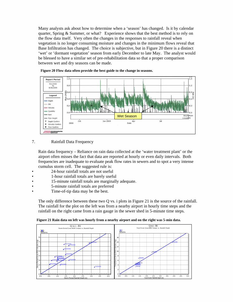
Many analysts ask about how to determine when a ‘season’ has changed. Is it by calendar quarter, Spring & Summer, or what? Experience shows that the best method is to rely on the flow data itself. Very often the changes in the responses to rainfall reveal when vegetation is no longer consuming moisture and changes in the minimum flows reveal that Base Infiltration has changed. The choice is subjective, but in Figure 20 there is a distinct ‘wet’ or ‘dormant vegetation’ season from early December to late May. The analyst would be blessed to have a similar set of pre-rehabilitation data so that a proper comparison between wet and dry seasons can be made.
7. Rainfall Data Frequency
Rain data frequency – Reliance on rain data collected at the ‘water treatment plant’ or the airport often misses the fact that data are reported at hourly or even daily intervals. Both frequencies are inadequate to evaluate peak flow rates in sewers and to spot a very intense cumulus storm cell. The suggested rule is:
• 24-hour rainfall totals are not useful • 1-hour rainfall totals are barely useful • 15-minute rainfall totals are marginally adequate. • 5-minute rainfall totals are preferred • Time-of-tip data may be the best.
The only difference between these two Q vs. i plots in Figure 21 is the source of the rainfall. The rainfall for the plot on the left was from a nearby airport in hourly time steps and the rainfall on the right came from a rain gauge in the sewer shed in 5-minute time steps.
Wet Season
Figure 20 Flow data often provide the best guide to the change in seasons.
(7/21/2009)
(7/29/2009)
(8/2/2009)
(9/26/2009)
(10/15/2009)
(10/23/2009)
(10/27/2009)
(12/2/2009)
(12/5/2009)
(12/9/2009)
(12/13/2009)
(12/25/2009)
(8/21/2009)
(8/28/2009) (9/11/2009)
0
1
2
3
4
5
6
7
8
0.0 0.5 1.0 1.5 2.0 2.5 3.0 3.5 4.0
Q vs i - B1Storm Period Gross RDII Volume vs. Rainfall Depth
Sto
rm P
eri
od
Gro
ss R
DII
Vo
lum
e (
mg
)
Storm Period Rainfall Depth (in)
AllStorms
(1/25/2010)
(2/22/2010)
(2/25/2010)
(3/12/2010)
(4/25/2010)
(5/3/2010)
(5/18/2010) (6/9/2010)
0
2
4
6
8
10
12
14
16
0.0 0.5 1.0 1.5 2.0 2.5 3.0 3.5 4.0 4.5 5.0
Q vs i - B1Total Event Gross RDII Volume vs. Rainfall Depth
To
tal E
ven
t G
ross
RD
II V
olu
me
(m
g)
Total Event Rainfall Depth (in)
AllStorms
Figure 21 Rain data on left was hourly from a nearby airport and on the right was 5-min data.

8. Pain of Subtraction
It is common for hydraulic modelers and newcomers to RDII studies to create a metering plan that places meters along trunk lines. Modelers do it because they are primarily interested in measuring flow at logical system nodes. Newcomers often do it in an attempt to reduce the number of meters and because they are not aware of the ‘Pain of Subtraction’. The result is that most of the flow calculations are obtained by subtracting one flow meter from another. Figure 22 shows the difference in the two approaches to meter placement. The plan on the left has 3 meters and the performance of most of the system is derived through subtraction. The plan on the right has 4 meters and the performance of most of the system is derived by direct measurement. The plan with fewer subtractions will produce more precise measurements of performance. In nearly all collection system flow studies, it is sometimes necessary to subtract a downstream meter from one or more upstream meters to isolate the net flow contribution from a basin. However, there are limitations to relying on such subtractions to yield net flows. This is due to the fact that as upstream meter flows are subtracted from downstream meter flows, the potential flow computation errors are additive among all of the associated meters. Figure 23 quantifies the Pain of Subtraction by showing the dramatic increase in potential error of the net flow calculation when net flows are a small percentage of total flow. In the best hydraulic conditions the subtraction of flow between accurate meters (±5%) to calculate net flows that are less than 30% of the total flow can introduce error greater than 20%.
S
S
S
M
M = MeasureS = Subtract
SM
S
M
M
S
M
S
M
M
M
S
M
M
S
Figure 22 Slight adjustments in locations result in more direct measurements.
0.0%
20.0%
40.0%
60.0%
80.0%
100.0%
120.0%
140.0%
0% 20% 40% 60% 80% 100%
Net Flow as a % of Total Flow
% e
rro
r in
Net
Flo
w C
alcu
lati
on
+/- 5% Meter +/- 20% Meter +/- 2% Meter Max Allowed Error
1.0 mgd
B
A 0.7 mgd
Net Flow = 1 – 0.7 or 30% of Total Flow
A
B
0.0%
20.0%
40.0%
60.0%
80.0%
100.0%
120.0%
140.0%
0% 20% 40% 60% 80% 100%
Net Flow as a % of Total Flow
% e
rro
r in
Net
Flo
w C
alcu
lati
on
+/- 5% Meter +/- 20% Meter +/- 2% Meter Max Allowed Error
1.0 mgd
B
A 0.7 mgd
Net Flow = 1 – 0.7 or 30% of Total Flow
A
B
Figure 23 Pain of Subtraction increases as net flow become a small percentage of total flow.

The concept for laying out meter basins and avoiding subtractions is summarized by the ‘10/20 Rule’, similarly referred to as “Graduated Basin Size Optimization”, Keefe, P., Doble, A., Rowe, R.(2009). The Rule considers only the length of public sewer lines in linear feet, because that information is the easiest to obtain (often from paper maps). The Rule considers all pipe sizes, but step 4 helps to overcome the problem of treating 36-inch pipe the same as 8-inch pipe. Keep in mind that around 85% of most sewer systems consist of 8-inch to 12-inch pipes. The 10,000 LF basin size can usually be maintained downstream into the 10-inch and 12-inch pipes and below that the meters are placed such that meter subtractions are no ‘tighter’ than 20%. The downstream basins necessarily will be larger (more LF of sewer). When following this rule for a large system it is possible that up to 60% of the total length of the system can be measured in small independent meter basins (no subtraction).
The 10/20 Rule
1. Treat sewer system like a tree with leaves, branches and a trunk.
2. Layout meter basins in the ‘leaves’ with 10,000 LF basins (approximate size of subdivisions)
3. Layout meters to avoid subtractions4. Make sure downstream meters are far
enough apart to create a ‘Net’ flow of at least 20% of the ‘Gross’ flow
5. Place meters upstream of modeling ‘nodes’or logical restrictions (e.g. siphons) to determine Operation Capacity
Figure 24 The 10/20 Rule for meter placement.
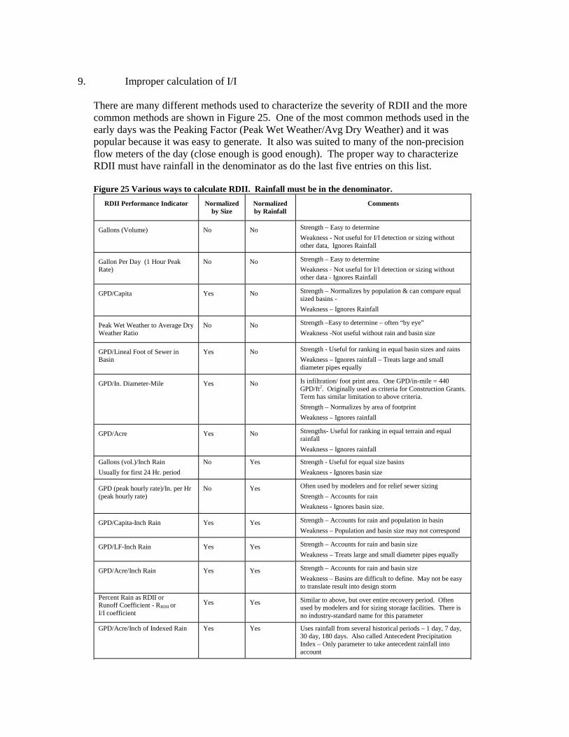
9. Improper calculation of I/I
There are many different methods used to characterize the severity of RDII and the more common methods are shown in Figure 25. One of the most common methods used in the early days was the Peaking Factor (Peak Wet Weather/Avg Dry Weather) and it was popular because it was easy to generate. It also was suited to many of the non-precision flow meters of the day (close enough is good enough). The proper way to characterize RDII must have rainfall in the denominator as do the last five entries on this list. Figure 25 Various ways to calculate RDII. Rainfall must be in the denominator.
RDII Performance Indicator Normalized by Size
Normalized by Rainfall
Comments
Gallons (Volume) No No Strength – Easy to determine
Weakness - Not useful for I/I detection or sizing without other data, Ignores Rainfall
Gallon Per Day (1 Hour Peak Rate)
No No Strength – Easy to determine
Weakness - Not useful for I/I detection or sizing without other data - Ignores Rainfall
GPD/Capita Yes No Strength – Normalizes by population & can compare equal sized basins -
Weakness – Ignores Rainfall
Peak Wet Weather to Average Dry Weather Ratio
No No Strength –Easy to determine – often “by eye”
Weakness -Not useful without rain and basin size
GPD/Lineal Foot of Sewer in Basin
Yes No Strength - Useful for ranking in equal basin sizes and rains
Weakness – Ignores rainfall – Treats large and small diameter pipes equally
GPD/In. Diameter-Mile Yes No Is infiltration/ foot print area. One GPD/in-mile = 440 GPD/ft2. Originally used as criteria for Construction Grants. Term has similar limitation to above criteria.
Strength – Normalizes by area of footprint
Weakness – Ignores rainfall
GPD/Acre Yes No Strengths- Useful for ranking in equal terrain and equal rainfall
Weakness – Ignores rainfall
Gallons (vol.)/Inch Rain
Usually for first 24 Hr. period
No Yes Strength - Useful for equal size basins
Weakness - Ignores basin size
GPD (peak hourly rate)/In. per Hr (peak hourly rate)
No Yes Often used by modelers and for relief sewer sizing
Strength – Accounts for rain
Weakness - Ignores basin size.
GPD/Capita-Inch Rain Yes Yes Strength – Accounts for rain and population in basin
Weakness – Population and basin size may not correspond
GPD/LF-Inch Rain Yes Yes Strength – Accounts for rain and basin size
Weakness – Treats large and small diameter pipes equally
GPD/Acre/Inch Rain Yes Yes Strength – Accounts for rain and basin size
Weakness – Basins are difficult to define. May not be easy to translate result into design storm
Percent Rain as RDII or Runoff Coefficient - RRDII or I/I coefficient
Yes Yes Similar to above, but over entire recovery period. Often used by modelers and for sizing storage facilities. There is no industry-standard name for this parameter
GPD/Acre/Inch of Indexed Rain Yes Yes Uses rainfall from several historical periods – 1 day, 7 day, 30 day, 180 days. Also called Antecedent Precipitation Index – Only parameter to take antecedent rainfall into account

Even EPA was late arriving at the conclusion that rainfall must be in the denominator of any RDII performance indicator. As late as 1991 EPA guidance was defining Excessive Infiltration and Excessive Inflow in terms of Gallons per Capita per Day. An analyst can extract RDII and rainfall information from data in many standard software packages including Microsoft Excel and other spreadsheets. Analysts who do this work regularly have developed spreadsheet templates the speed up this work. At the least the data that should be extracted form each storm are shown in Figure 27.
Criteria Source EPA Program Requirements Memorandum (PRM 78-10, 1978)Draft Program Requirements Memorandum (PRM) 80 ,1980
Non-Excessive Rate Length of Sewer 2,000-3,000 gpdim >100,000 lf 3,000-5,000 gpdim 50,000-100,000 lf 5,000-8,000 gpdim 1,000-50,000 lf
Non-Excessive Rate Length of Sewer 2,000-3,000 gpdim >100,000 lf 3,000-6,000 gpdim 10,000-100,000 lf 6,000-10,000 gpdim <10,000 lf
No operational problems in collection system and WWTPSource: ASCE, 2004, "Sanitary Sewer Overflow Solutions," Black & Veatch, EPA Cooperative Agreement #CP-828955-01-0
Preceding year’s 7-14 day high groundwater wastewater flow < 120 gpcdNon-Excessive InflowTotal daily average storm flow < 275 gpcd
EPA Handbook: Sewer System Infrastructure Analysis and Rehabilitation EPA 625/6-91/030, 1991
Non-Excessive Allowance RangesEPA Handbook: Procedures for Investigating Infiltration/Inflow, EPA 68-01-4913, 1981
EPA Handbook: Facilities Planning, 1981
Non-Excessive Infiltration
Selected Historical Excessive Infiltration Inflow Criteria Criteria for Non-Excessive Infiltration Determination
Established 1500 gpdim as non-excessive leakage allowance, perform a cost-effective analysis to determine if the leakage is possibly excessive and Proposed 3,000 gpdim as non-excessive allowance, maximum of 30%infiltration removal for use in cost-effectiveness analysis (CEA)
Figure 26 Summary of how EPA characterized RDII.
0.166 in/hr 14:00
Storm Event - 3/13/2010 10:00:00 AM330038
Ra
infa
ll (in)F
low
(M
GD
)S
torm
s
Date13 Sat
Mar 201014 Sun 15 Mon 16 Tue 17 Wed
0.00
0.02
0.04
0.06
0.08
0.10
0.12
0.14
0.16
0.18
0.20
0.22
0.0
0.2
0.4
0.6
0.8
1.0
1.2
1.4
1.6
1.8
2.0
2.2
0.00.51.0
Rainfall Gross Q Gross I/I Precomp(-) Weekends Weekdays
Peak Rainfall Peak
RDII
RDIIHydrograph
RainfallHyetograph
Dry Day HydrographWeekend & Weekday
FlowHydrograph
Figure 27 The basic calculations that should be conducted for every storm.

Stevens and Tutton (2010) have described how Sliicer.com allows users to reduce the analysis processing time by intelligently performing many of the basic calculations required in an RDII analysis. Sliicer.com was the recipient of the WEF’s 2009 Innovative Technology Award. The software is available for use on-line for anyone with flow and rain data and it produces five key views of these data as shown in Figure 28.
Importantly, Sliicer.com can also automatically produce strong RDII metric results that can be used to identify basins with excessive RDII, without relying on weaker knee-of-the-curve prioritization approaches. Elaborate?
Figure 28 The Five Views of Flow and Rain Data
Flow Data
Rain Data
0.7
0.8
0.9
1.0
1.1
1.2
1.3
1.4
0 3 6 9 12 15 18 21
Dry Weather FlowWeekdays, Fridays and Weekends
MG
D
Hours
Weekdays Weekends Friday
Dry Day SelectionUses Antecedent Rain Estimate Base InfiltrationUse in Model
RDII DecompositionPrecompensationMeasure Peak and Volumes
Storm Event - 04/28/94 22:00GV04
Ra
infa
ll (Inc
he
s)
Flo
w (
mg
d)
Sto
rms
Date
0.00
0.05
0.10
0.15
0.20
0.25
0.30
0.35
0.0
0.5
1.0
1.5
2.0
2.5
3.0
3.5
4.0
4.5
0.00.51.0
27 WedApr 94
28 Thu 29 Fri 30 Sat 1 May 2 Mon
Rainfall Gross Q Gross I/I Net I/I
Precomp(-) Weekdays Weekends
Net RDII hydrograph obtained by subtracting upstream meter(s) from the gross hydrograph.
(2/20/2003)
(1/26/2003)
(2/6/2003)
(2/14/2003)
0.0
0.2
0.4
0.6
0.8
1.0
1.2
0.0 0.5 1.0 1.5 2.0 2.5 3.0 3.5 4.0 4.5
Q vs i - PN06Storm Period Net RDII Volume vs. Rainfall Depth
Sto
rm P
eri
od
Ne
t R
DII
Vo
lum
e (
mg
)
Storm Period Rainfall Depth (in)
AllStorms
Rain-to-RDII RelationshipVolume & Peak PlotsCapture CoefficientRDII Predictions
ScattergraphsOperational CapacityHydraulic ObstructionsOverflows
DDF AnalysisReturn FrequencyDurations
1
2
3
4
5
6
7
15 20 30 60 120
180
1080
360
720
1440
2880
DDF Graph
Rai
nfal
l (in
)
Duration (min)
RG01-8/27/2009 10:00:00 PM RG04-8/27/2009 10:00:00 PM RG10-8/27/2009 10:00:00 PM
1-year 2-year 5-year
10-year 25-year 50-year
25.7-year, 2-hr, 2.7 in.
44.4-year,3-hr, 3.2 in.
2.8-year,24-hr, 3.3 in.
0
1
2
3
4
5
6
7
8
9
10
0 10 20 30 40 50 60 70 80
0.2
0.8
1.6
2.4
3.2
4
4.8
5.6
6.4
7.2
Scatter GraphLS115
VF
INA
L (f
t/s)
Iso Q (M
GD
)
DFINAL (in)
Lanfear-Coll (C-LC = 13.04)

10. Restricted Sewer - Potential I/I
Kurz 2010 has demonstrated that a Q vs i relationship should be linear provided the data are from similar hydrologic seasons and the sewer is not hindered or restricted. To most people the concept of a hindered or restricted sewer means that the sewer, at or downstream of the meter, is backed up or surcharged. But what if the restriction or hindrance is upstream of the meter? It is the shape or non-linearity of the Q vs i plot that alerts us to this problem. Figure 29 shows the case in which a restriction and an upstream loss of flow can be detected in the scattergraph of a flow meter. In this scattergraph we see that not only is the pipe restricted to around 50% of its capacity, but also there is lost RDII upstream through an SSO at a depth of 126 inches as measured in the metering manhole. In this situation both the flow rate and flow volume will reach some upper limit, regardless of the amount of rainfall.
Kurz and Hegwald discuss the phenomenon of ‘Potential RDII; and explain how it may result in the rate of RDII being higher after rehabilitation than before. Figure 30 shows that after reaching a certain rainfall amount, the sewers become surcharged and no additional RDII may enter. Kurz and others have recommended that RDII measurements collected during surcharge (restricted flow) not be included in a regression analysis. In this example, the initial study measured 11 mgd of RDII when the actual amount of RDII available to enter was 30 mgd. The sewer capacity may have increased after rehabilitation and the unmeasured “Potential RDI/I” may enter the sewer allowing an even
QA/QC Upstream SSO
Upstream SSO
Depth - VelocityFlowmeter ROOTS
SSO Upstream of Flowmeter
Figure 28 The scattergraph reveals both a restricted pipe and an upstream overflow.
Rainfall vs. RDII
0
5
10
15
20
25
30
0 1 2 3 4 5 6
Rainfa ll - In.
RD
II -
mg
d.
Projected Flow
Pipe Capac ity
Restric ted Flow
Po
ten
tial R
DII
Figure 30 Restricted sewer with Potential RDII

greater amount of RDII to be measured. In fact, Hegwald suggests that if sewer rehabilitation is successful and total RDII is reduced, the peak rate of RDII recorded at a site with low operational capacity should be expected to increase, because the sewer’s operational capacity has been increased by cleaning and perhaps lining. In this case an investigator looking at merely peak to average ratios as a performance indicator, will see an “after” picture worse than the “before” picture.
However if the restriction and overflow occur upstream of the flow meter, it is only the Q vs. i plot that will reveal the presence of ‘Potential RDII’ in the basin It is often a cruel surprise for agencies that are not accustomed to using the Q vs. i plot as a Key Performance Indicator.
11. Control Basins An agency contemplating significant sewer rehabilitation should set up one or more control basins of similar size (say 5,000 to 15,000 LF) as the basins to be rehabilitated. The control basin should be in the same area of the collection system, in the same soil type, etc. There should be measurable RDII in the control basin so changes can be observed over time. For example if the agency’s program strategy is to perform rehabilitation on any basis with RDII severity of a Capture Coefficient of 7% or greater, the control basin should have RDII severity of around 7%. The control basin serves the same function as a laboratory blank does in chemistry. The control basin should be left alone with no rehabilitation. The control basin helps account for the differences between a wet pre-rehab period and a dry post rehab period or vice versa.5 Engineers who have tried to compare before and after rainfall and flow data from sewer rehabilitation projects know the difficulties and frustrations associated with trying to reach a simple conclusion. Many factors affect the rainfall-to-runoff relationship in sanitary sewers so there is inevitably a wide scatter in the data. Factors most affecting the rainfall to runoff relationship within a basin include: 1) rainfall intensity, 2) antecedent moisture, 3) season, 4) storm duration, 5) surface water flooding, 6) snowmelt, and 7) new construction or rehabilitation. In fact, the scatter caused by these 7 variables is often so wide that a simple comparison of a month’s worth of I/I before rehab to a month’s worth of I/I after rehab is highly unlikely to capture the true effectiveness of rehabilitation. The solution is to collect data from many, many storms before, during and after rehab. It is important that the control basin experiences as few changes as possible throughout the pre- and post-rehabilitation. For that reason a drift-free flow meter and rain gauge(s) should remain in place for the whole period. One respondent to the question ‘having this to do over’ said that if that agency cannot leave the meter in place for the entire period; the post-
Control Basins Insure Valid Results and Remove Seasonal Bias
• Same concept as a laboratory control.
• Similar era.
• Similar construction
Control Monitor
Control RG
Control Basin
Rehabilitated Basin
Figure 31 Control basin should be in same area.

rehab meters should be the very same meter, installed by the very same company and if possible by the very same person. The goal is to eliminate and may variables as possible.
12. Poor Hydraulics at Metering Site It is common for analysts to ask about flow meter accuracy and nearly all flow meter manufacturers will say the meter is 95% accurate (± 5% error) despite the fact that most have not been tested in the EPA Environmental Testing and Verification program. The analyst assumes that the data from the sewer will have an error of 5% or less regardless of the flow conditions in the metering sewer. The assumption in open-channel flow metering is that flow has a constant velocity and cross sectional area as it approaches and passes by the meter. Conditions that interfere with this assumption are offset joints, unevenly sloped pipes, drops into the manhole, hydraulic jumps in the sewer, Dead Dogs in the sewer, varying silt, excessive surcharging, etc. The actual error in these conditions can easily be up to 25% or 50% and much higher in combined sewers. Of course such metering locations are often unavoidable, but the mistake is to insist on metering in such sites in the belief that a ± 5% value can come from a ± 25% site. When the work is over the analyst cannot extract the information being sought. These are self-inflicted wounds often committed by the most brilliant engineers and scientists.

CONCLUSIONS The authors have been involved in several ‘Forensic RDII’ evaluations in an effort to figure out why pre-and post-rehabilitation data do not demonstrate that RDII was removed. Typically the greatest cause of the failure is the use of rain data from too-distant rain gauges followed by inaccurate and insufficient flow data. In third place is the inability to deploy the Key Performance Indicators for the extraction RDII information in a systematic way. Sliicer.com offers this ability to any agency and any analyst. The table below summarizes the 12 items in the recipe for successful measurement of sewer rehabilitation effectiveness.
Figure 32 RDII Project Elements to Specify as a Minimum
RG Strategy At least 1 every 4 sq. miles in grid
Duration Minimum of 90 days
QA/QC Touchstones KPIs
Make sure Scattergraphs and Q vs i plots are deliverables.
Metering depth Ultrasonic Depth technology - pressure backup
Basin Size 10,000 LF Upper end - 20% Net subtraction down
Season Start in dry - end in wet
RG data Five-minute time steps
Pain of Subtraction Net Subtraction no less than 20% of Gross flow
RDII Calculation Capture Coefficient and Gallons/inch/LF (rainfall in the denominator)
Sewer Dynamics Scattergraph and Q-i will spot restricted sewers and Potential RDII
Control basin Identify at beginning & Use to evaluate pre- and post metering of rehabilitated basins.
Site Hydraulics Avoid Silt, Hydraulic Jumps and Dead Dogs. Believe the flow monitoring folks when they tell you a site is bad for metering.

REFERENCES
Stevens, P.L. (1997). The Eight Types of Sewer Hydraulics. Proceedings of the Water Environment Federation Collection Systems Rehabilitation and O&M Specialty Conference; Kansas City, MO. Water Environment Federation: Alexandria, VA. Schutzbach, J., Stevens P.L. (1998). New Diagnostic Tools Improve the Accuracy of the Manning Equation. Proceedings of the Water Environment Federation Collection Systems Specialty Conference, Houston TX.
Stevens, P.L. (2000). Peeling the Onion of Meter Accuracy – Two Steps to Evaluating Flow Meter Data. Proceedings of the Water Environment Federation WEFTEC Conference, Atlanta GA Kurz, G., Stevens, P., Ballard G. (2002). Flow Knowledge – Tools for Sewer Operation and Targeting Renewal. Proceedings of CSCE/EWRI of ASCE Environmental Engineering Conference, Niagara, ON. Enfinger, K.L. and Keefe, P.N. (2004). Scattergraph Principles and Practice – Building a Better View of Flow Monitor Data. KY-TN Water Environment Association Water Professionals Conference; Nashville, TN. Enfinger, K.L. and Kimbrough, H.R. (2004). Scattergraph Principles and Practice -A Comparison of Various Applications of the Manning Equation. Proceedings of the Pipeline Division Specialty Conference, San Diego, CA. America Society of Civil Engineers. Enfinger, K.L., Stevens P.L. (2005) Scattergraph Principles and Practice Poster. Published by ADS Environmental Services, Huntsville AL
Enfinger, K.L. and Stevens, P.L. (2006). Scattergraph Principles and Practice – Tools and Techniques to Evaluate Sewer Capacity. Proceedings of the Pipeline Division Specialty Conference; Chicago, IL; American Society of Civil Engineers: Reston, VA. Enfinger, K.L. and Stevens, P.L. (2007). Scattergraph Principles and Practice – Characterization of Sanitary Sewer and Combined Sewer Overflows. Proceedings of the Pipeline Division Specialty Conference; Boston, MA; American Society of Civil Engineers: Reston, VA. Mitchell, P.S., Stevens, P. L., Nazaroff, A. (2007). A Comparison of Methods and a Simple Empirical Solution to Estimating Base Infiltration in Sewers. Water Practice Vol. 1 No. 6 Water Environment Federation
Keefe, P., Doble, A., Rowe, R. (2009). “Graduated Basin Size Optimization,” Proceedings fo the Water Environment Federation, WEFTEC Conference, 2009. Kurz, G.E., Hamilton, W.P. (2010). Confidence Levels for Estimating RDI/I. Proceedings of the Water Environment Federation WEFTEC Conference, New Orleans, LA.

Stevens, P.L., Tutton, D.L. (2010). ‘Extracting Hydraulic Performance & I/I Information at Human Viewing Speed’. Proceedings of the Water Environment Federation WEFTEC Conference, New Orleans LA Stevens, P.L. (2011). Recipe for Successful Measurement of RDII Reduction. Water Utility Infrastructure Management (UIM) Webinar.