iem unit 2

7/28/2019 IEM UNIT 2

http://slidepdf.com/reader/full/iem-unit-2 1/116

DEMAND & DETERMINANTS OF

DEMAND

7/28/2019 IEM UNIT 2


DEFINITION OF DEMAND Demand is different from mere desire. Actually the desire is only

a wish to get things but demand requires willingness to pay as well as ability to pay.

Definition-The demand means a desire backed by willingness

and ability to pay.

The demand for any commodity is the quantity of it a consumerdecides to buy at a given price and at a given time.

For eg a beggar has a desire to own a house but he does not have willingness and ability to pay then that is not called demand. Buta business man has desire to own a house. He has willingness as

well as ability to pay then that is called as demand.

7/28/2019 IEM UNIT 2


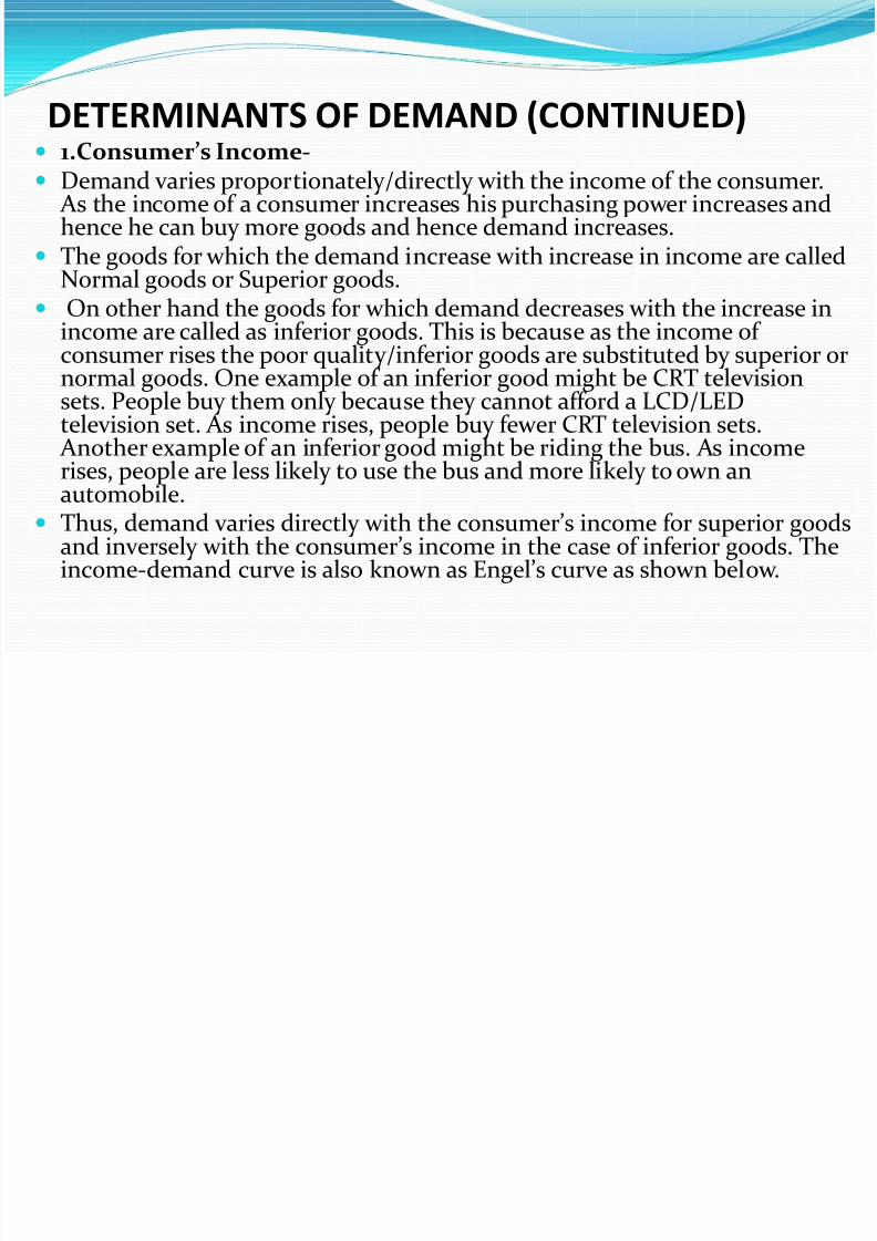
DETERMINANTS OF DEMAND (CONTINUED) 1.Consumer’s Income- Demand varies proportionately/directly with the income of the consumer.

As the income of a consumer increases his purchasing power increases andhence he can buy more goods and hence demand increases.

The goods for which the demand increase with increase in income are calledNormal goods or Superior goods.

On other hand the goods for which demand decreases with the increase inincome are called as inferior goods. This is because as the income of consumer rises the poor quality/inferior goods are substituted by superior ornormal goods. One example of an inferior good might be CRT televisionsets. People buy them only because they cannot afford a LCD/LEDtelevision set. As income rises, people buy fewer CRT television sets.

Another example of an inferior good might be riding the bus. As incomerises, people are less likely to use the bus and more likely to own anautomobile.

Thus, demand varies directly with the consumer’s income for superior goodsand inversely with the consumer’s income in the case of inferior goods. Theincome-demand curve is also known as Engel’s curve as shown below.

7/28/2019 IEM UNIT 2


DETERMINANTS OF DEMAND

Income

Demand for Superior/Normal Goods

Engel’s Curve

Income

Demand for Inferior Goods

7/28/2019 IEM UNIT 2


DETERMINANTS OF DEMAND (CONTINUED) 2.Price of Related Goods- a. Price of same good

Normally the demand for a commodity varies inversely with its own price.Thus, other things remaining constant the demand for a good increases asits price decreases and vice versa. This is also known as law of demand. A

graphical representation is shown below-

Price

Demand for Goods

7/28/2019 IEM UNIT 2


DETERMINANTS OF DEMAND (CONTINUED)

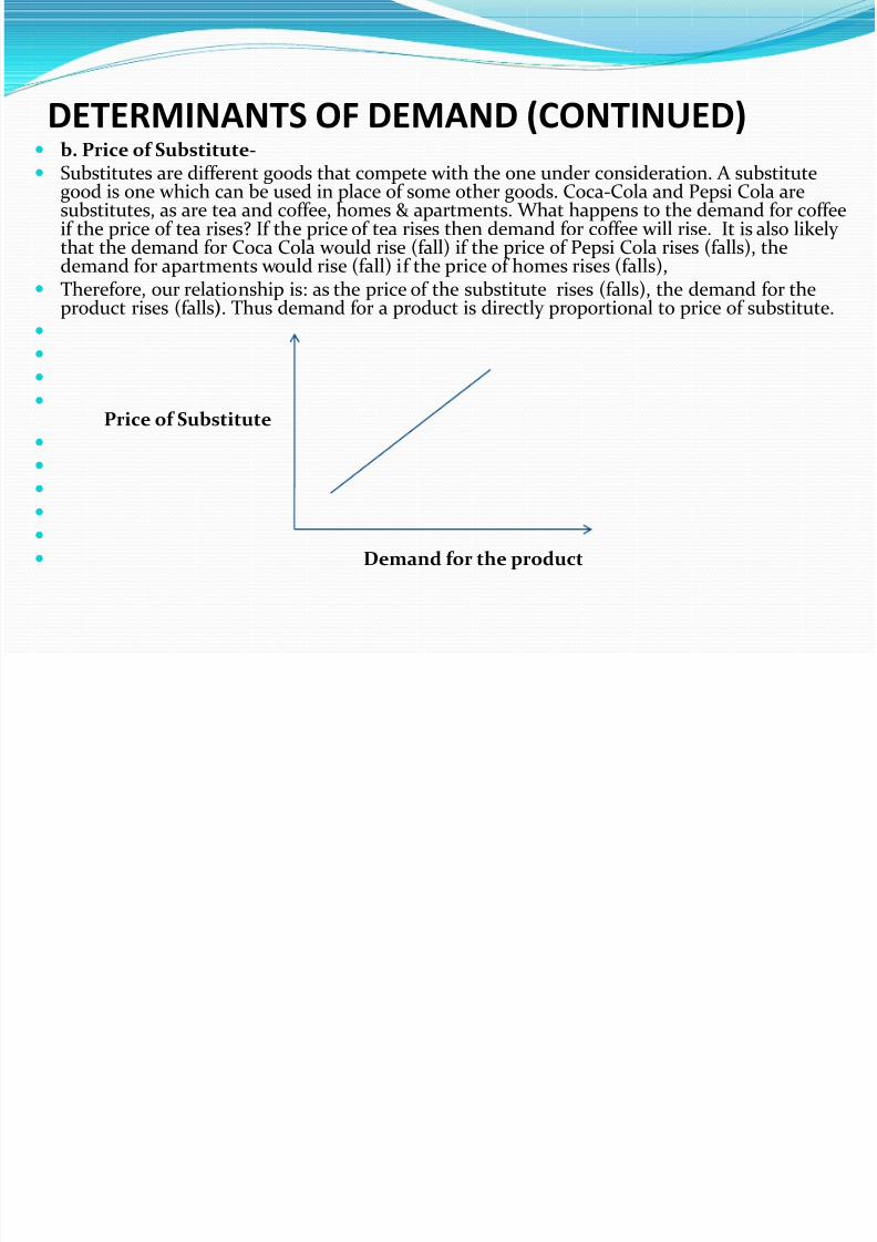
b. Price of Substitute- Substitutes are different goods that compete with the one under consideration. A substitute

good is one which can be used in place of some other goods. Coca-Cola and Pepsi Cola aresubstitutes, as are tea and coffee, homes & apartments. What happens to the demand for coffeeif the price of tea rises? If the price of tea rises then demand for coffee will rise. It is also likely that the demand for Coca Cola would rise (fall) if the price of Pepsi Cola rises (falls), thedemand for apartments would rise (fall) if the price of homes rises (falls),

Therefore, our relationship is: as the price of the substitute rises (falls), the demand for the

product rises (falls). Thus demand for a product is directly proportional to price of substitute.

Price of Substitute Demand for the product

7/28/2019 IEM UNIT 2


DETERMINANTS OF DEMAND (CONTINUED) c.Price of Complement A complement is a different good that goes together with the

one under consideration.

Homes and interest rates tend to go together. So do bread and

butter, tea and sugar, petrol and automobiles. What happens to the demand for new homes if the interest rate

rises? The answer, of course, is that it falls.

When interest rates rise, people are less likely to borrow. If they do not borrow, they will not buy the homes.

It is also likely that the demand for sugar will fall if the price of tea rises, the demand for automobiles will fall if the price of petrol rises, and so on.

Therefore, our relationship is: if the price of the complement

rises (falls), the demand for the product (homes) falls (rises).

7/28/2019 IEM UNIT 2


DETERMINANTS OF DEMAND (CONTINUED) 3. Consumer’s Tastes and Preferences- Another determinant of demand is one’s taste and preference.

Taste and preference are influenced by culture, religion, socialcustoms, habits of people, lifestyle, age, gender and history.

For example eating beef is popular in America but it is a tabooin India.

The principle is: the more (less) we like a good or service, thegreater (less) is our demand for it.

For example if you like ice cream you buy more of it. If consumers taste or preference change for certain goods and

services following change in fashion, people switch theirconsumption pattern from cheaper old fashioned goods over to

costlier modern goods.

7/28/2019 IEM UNIT 2


DETERMINANTS OF DEMAND (CONTINUED) 4. Expectations Expectations affect our demand for many products. For

example, people commonly buy Shares/Land because they expect the prices of the shares or land to rise. The principle

here is: if buyers expect the price to rise (fall), the demand rises(falls) today.

There are other kinds of expectations one might have that willaffect the demand for products.

If one expects that the product will soon be unavailable, thedemand will rise today. This is the case for petrol/diesel if Oilcompanies go on strike. Expecting that petrol stations will beclosed, buyers rush to stock-up. Also, if one expects that one's

income will rise, he will start saving less and spending more.

7/28/2019 IEM UNIT 2


DETERMINANTS OF DEMAND (CONTINUED) 5. Population/Number of Buyers The market demand is simply the sum of the individual

demands. If the population or number of buyers rises then themarket demand is bound to rise.

It because of rising population of India and China many MNCs

want to enter into Indian & Chinese market. The population of there home country is on decline and so is the demand for theirproducts.

6.Distribution of National income- The distribution pattern of national income also affects the

demand for a commodity. If the national income is evenly distributed market demand for normal goods will be highest. If the national income is unevenly distributed i.e. if majority of population belongs to lower income groups, market demand

for essential goods (including inferior ones) will be highest.

7/28/2019 IEM UNIT 2


DETERMINANTS OF DEMAND

(CONTINUED) Demand Function

Dx = f( Px, Pr, I, T, E)

Px- Price of a commodity

Pr-Price of related goods

I-Income of the consumer

T-Taste of the consumers

E-Expectations

7/28/2019 IEM UNIT 2


Law of Demand Law of Demand-“Other things being equal at any

given time demand for a commodity or service rises with decrease in price and falls with increase in price.

Demand Schedule

-A table showing differentquantities demanded by an individual consumer ornumber of consumers of a commodity at differentprices is known as demand schedule.

Demand Schedule for Sugar at different prices-

Price in Rs 40 35 30 25 20

Demand inKgs

1 1.5 2 3 5

7/28/2019 IEM UNIT 2


Law of Demand (Continued)

Price

Demand for Goods

7/28/2019 IEM UNIT 2


Exceptions/Limitations of Law of Demand There are some cases where the demand for a good varies directly

with its own price. These cases are exceptions to law of demandor limitations of law of demand.

Giffen Goods /Giffens Paradox- Sir Robert Giffen of Ireland first observed that people used to

spend more their income on inferior goods like potato and less of

their income on meat. But potatoes constitute their staple food. When the price of potato increased, after purchasing potato they did not have so many surpluses to buy meat. So the rise in priceof potato compelled people to buy more potato and thus raisedthe demand for potato. This is against the law of demand. This isalso known as Giffen paradox.

These goods are inferior goods consumed mostly by poorconsumers as essential commodities e.g. bajra. Consumers spenda considerable portion of limited income on these goods. Thedemand for such goods increases with an increase in price anddecreases with decrease in price.

7/28/2019 IEM UNIT 2


Exceptions/Limitations of Law of Demand

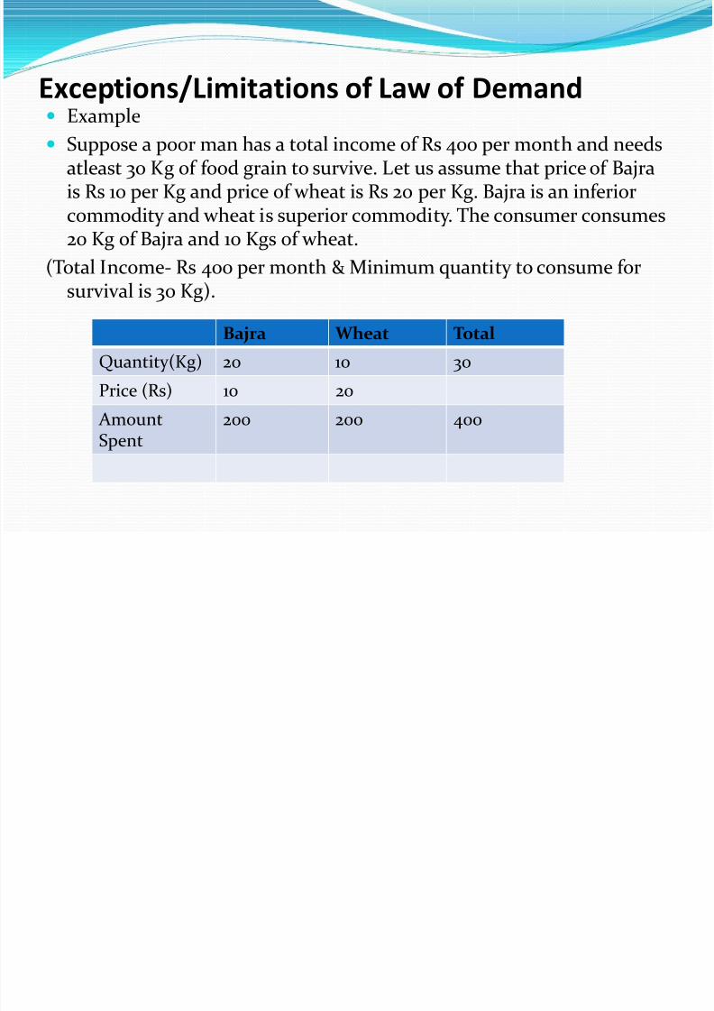
Example Suppose a poor man has a total income of Rs 400 per month and needs

atleast 30 Kg of food grain to survive. Let us assume that price of Bajrais Rs 10 per Kg and price of wheat is Rs 20 per Kg. Bajra is an inferiorcommodity and wheat is superior commodity. The consumer consumes20 Kg of Bajra and 10 Kgs of wheat.

(Total Income- Rs 400 per month & Minimum quantity to consume forsurvival is 30 Kg).

Bajra Wheat Total

Quantity(Kg) 20 10 30

Price (Rs) 10 20

AmountSpent

200 200 400

7/28/2019 IEM UNIT 2


Exceptions/Limitations of Law of Demand

If the price of Bajra rises to Rs 12 per Kg while that of wheat remains the same.

(Total Income- Rs 400 per month & Minimum quantity toconsume for survival is 30 Kg).

Thus we can see that when price of Bajra rises theconsumer raises the quantity of Bajra from 20 Kg to 25 Kgand reduces the quantity of wheat from 10 Kg to 5 Kg toconsume minimum required quantity of 30 Kg for survival

with his stipulated income of Rs 400.

Bajra Wheat TotalQuantity(Kg) 25 (20) 5(10) 30

Price(Rs) 12 (10) 20 (20)

AmountSpent

300 100 400

7/28/2019 IEM UNIT 2


Exceptions/Limitations of Law of Demand If the price of Bajra falls to Rs 8 per Kg while that of wheat

remains the same. (Total Income- Rs 400 per month & Minimum quantity to consume for

survival is 30 Kg)

Thus we can see that when price of Bajra falls then he uses this savingdue to fall in price of Bajra to purchase greater quantity of wheat (10 Kgto 13.3 Kg) and lowers the quantity of Bajra from 20 Kg to 16.7 Kg toconsume minimum required quantity of 30 Kg for survival with hisstipulated income of Rs 400.

Thus in case of Giffens Goods the demand for a commodity increases with the increases in it’s price and falls with fall in the price.

Bajra Wheat Total

Quantity(Kg) 16.7 (20) 13.3 (10) 30

Price(Rs) 8 (10) 20 (20)

AmountSpent

133.6 266.6 400

7/28/2019 IEM UNIT 2


Exceptions/Limitations of Law of Demand Costly Luxury goods or Veblen Goods Luxury goods are those that are not essential for the survival of human beings. Thus

goods like diamonds, antiques, air conditioners etc are luxury goods. For such goodsthe demand increases with an increase in the price and vice versa. This is becauserich people attach a lot of value to costly luxury goods that distinguish them fromcommon people. These goods have a prestige value for the upper strata of society. Whenever the price of such goods rises, their prestige value increases and hence thedemand for them goes up.

Necessities: Certain things become the necessities of life. So we have to purchasethem despite their high price. The demand for Sugar, Wheat etc. has not gonedown in spite of the increase in their price. So they are purchased despite theirrising price

Emergencies: Emergencies like war, famine etc. negate the operation of the law of demand. At such times, households behave in an abnormal way. Householdsaccentuate scarcities and induce further price rises by making increased purchaseseven at higher prices during such periods. During depression, on the other hand, nofall in price is a sufficient inducement for consumers to demand more.

7/28/2019 IEM UNIT 2


Exceptions/Limitations of Law of Demand Future changes in prices: Households also act speculators. When the prices are rising

households tend to purchase large quantities of the commodity out of the apprehension that prices may still go up. When pricesare expected to fall further, they wait to buy goods in future atstill lower prices. So quantity demanded falls when prices are

falling. Change in fashion Outdated goods: A change in fashion and tastes affects the market for a

commodity. Goods that go out of use due to advancement intechnology or change in tastes of consumer are called outdatedgoods. For example demand for CRT television sets, radio and

telephone will fall even if their prices fall. Seasonal Goods Seasonal goods which are not used during the off season will be

subject to similar demand behaviour. For example sale of aircoolers may go down in winters even if they are sold at reduced

prices.

7/28/2019 IEM UNIT 2


7/28/2019 IEM UNIT 2


Income Elasticity of Demand

The income elasticity of demand is the measure of thepercentage change in the demand of a commodity to thepercentage change in consumer’s income ceteris paribus(Other things remaining constant)

Ei= Percentage change in demand/Percentage change inincome.

It is positive when demand has a direct relationship with

consumer’s income in case of normal and superior goodslike LCD/LED television

7/28/2019 IEM UNIT 2


Income Elasticity of Demand

Income

Demand for Goods(Normal or Superior Goods)

It is negative when demand has inverse relationship with consumer’sincome in case of inferior goods lke CRT televisions.

Income

Demand for Inferior Goods

7/28/2019 IEM UNIT 2


7/28/2019 IEM UNIT 2


Price Elasticity of Demand

The ratio of proportionate change in quantity demanded to proportionate change in price is calledelasticity of demand. It measures the responsiveness of demand for a product to the changes in the price of

product, when all other variables are constant Price Elasticity of Demand=Ep=

Proportionate Change in Quantity Demanded

Proportionate Change in Price=Q1- Q2/P1-P2

7/28/2019 IEM UNIT 2



Perfectly Elasticity of Demand (Infinite) When negligible fall or rise in price of commodity

leads to great/infinite extension/contraction indemand it is called perfectly elastic demand.

Price Ep=∞

Quantity Demanded

7/28/2019 IEM UNIT 2



Perfectly Inelastic Demand(Zero Elasticty)- When great rise/fall in price of commodity does not

cause any considerable rise or fall in demand it iscalled perfectly inelasticity or zero elasticity.For eg Salt

and Life Saving drugs.

. Price Ep=0

Quantity Demanded

7/28/2019 IEM UNIT 2



Highly Elastic Demand- When a small rise/fall in price causes substantial or

considerable contraction/expansion in quantity demanded then that is called highly elastic demand.

Price Ep > 1

Quantity demanded

7/28/2019 IEM UNIT 2


7/28/2019 IEM UNIT 2


Cross Elasticity of Demand

Cross Elasticity of Demand- Demand for a product seldom exists in isolation and often price of some related product also

causes a variation in the demand for a commodity. Either it can be substitute or complement. A substitute good is one which can be used in place of some other goods. Coca-Cola and Pepsi

Cola are substitutes, as are tea and coffee, homes & apartments. A complement is a different good that goes together with the one under consideration. Homes

and interest rates tend to go together. So do bread and butter, tea and sugar, petrol andautomobiles.

It would therefore become important for a manager to develop some sort of relationshipbetween demand for a commodity and price of related goods. This can be done by knowing thecross elasticity of demand. The cross elasticity of demand measures the responsiveness of demand for one product to the changes in price of another.

Ec= Percentage change in demand of X/ Percentage change in price of Y where X an Y are either substitutes or complements.

The cross elasticity of demand is positive for substitutes and negative for complements. In case of substitutes tea and coffee if the price of tea rises and coffee remains the same, then

people will replace tea with coffee and so the demand for coffee will rise. Thus demand forcoffee increases with rise in price of substitute tea. Thus the direct relationship makes the crosselasticity positive.

In case of complements Cars and interest rates if the interest rates rises then people willpostpone their purchases of cars and so demand for cars decreases with rise in complementinterest rates. Thus the inverse relationship makes the cross elasticity negative.

7/28/2019 IEM UNIT 2


7/28/2019 IEM UNIT 2


Determinants of Price Elasticity of Demand 1.Availability of Substitutes- The closer the substitute greater is the elasticity of demand for that

commodity. For example tea and coffee are close substitutes. So if price of tea rises and coffee remains the same then demand for tea will fall morethan the proportionate increase in price because the consumer have optionof switching to cheaper substitutes.

2. Nature of Commodity- Commodity can be classified as luxuries, comforts and necessities and

nature of commodity affects the price elasticity of demand. Luxuries- Demand for luxuries (luxury cars, decorative items) is more

elastic than demand for other goods because consumption of these goodscan be postponed if the price of such commodity rises. Necessities- Consumption of necessary goods (eg sugar, clothes,

vegetables etc) cannot be postponed and hence their demand is inelastic. Comforts- Demand for comforts ( Air conditioners, Washing machines) is

more elastic than necessaries but less elastic than luxuries.

7/28/2019 IEM UNIT 2


7/28/2019 IEM UNIT 2


Determinants of Price Elasticity of Demand 5. Range of Alternative Uses of a Commodity

The wider the range of alternative uses of a product, thehigher the price elasticity of its demand for decrease in

price but less elastic for the rise in price. As the price of amulti-use commodity decreases, people extend theirconsumption to its other uses. Therefore the demand forsuch a commodity generally increases more than theproportionate decrease in its price. For instance milk can

taken as it is, it may be converted into curd, cheese, gheeand butter milk. The demand for milk will be highly elasticfor decrease in price but will be in elastic to increase inprice.

7/28/2019 IEM UNIT 2


Point Elasticity & Arc Elasticity The elasticity of demand is measured either at a finite point or

between any two finite points on the demand curve. Point Elasticity of Demand- It is defined as the proportionate

change in quantity demanded in response to a very small

proportionate change in price or the elasticity measured on afinite point of a demand curve is called point elasticity. Ep= Q1-Q2/Q1 =Q1-Q2/Q1 x P1/P1-P2 P1-P2/P1 For eg The demand for a product priced between Rs 10/unit and

Rs 8/unit is 200 and 400 units. Then Q1= 200 units , Q2=400 units & P1= Rs 10/unit , P2= Rs 8/unit Point elasticity at P1 = 200-400/200 x 10/10-8 =-5 Point elasticity at P2= 200-400/400 x 8/10-8

= -2

7/28/2019 IEM UNIT 2


Point Elasticity & Arc Elasticity Arc Elasticity of Demand- It is measure of the average of

responsiveness of the quantity demanded to a substantialchange in price or the elasticity measured between any twofinite points is called arc elasticity.

Ea= Q1-Q2/Q1+Q2/2P1-P2/P1+P2/2

For eg The demand for a product priced between Rs 10/unitand Rs 8/unit is 200 and 400 units. Then Q1= 200 units ,Q2=400 units & P1= Rs 10/unit , P2= Rs 8/unit

Arc Elasticity = 200-400/200+400/2 10-8/10+8/2 = -3

7/28/2019 IEM UNIT 2


Supply & Determinants of Supply Supply-It is quantity of commodity which is offered

for sale at a particular rate and time.

In simple words it means the quantities that a seller is willing and able to sell at different prices.

Determinants of Supply/Factors on which Supply depends-

Price of the Product- The supply of a product

depends upon the market price of that product. If theother things are same, a higher price of the product would make its production more profitable. So as theprices rises supply increases and vice versa.

7/28/2019 IEM UNIT 2


7/28/2019 IEM UNIT 2


Determinants of Supply Factor Prices- Since the prices of the factors of production are

costs from the point of view of the firm, a rise in their pricesresults in pushing up the costs of production. The profit margindeclines and the supply also falls.

State of Technology- This also influences the supply of goods.

Sometime new technology is developed which lowers the cost of production which in turn increases the supply. Sometimes newproducts are invented which affect the supply of existingproducts. For example Chemistry made available to us several

varieties of plastic as a result of which the supply of many

products like bamboo-baskets has declined. Future Expectations of Price- If the seller expects the price to

rise further in the future then he might lower the supply ormaintain it at the same level even if the price might have risen.

When further heavy fall in price is anticipated the seller may

become panicky and sell more at a current lower price.

7/28/2019 IEM UNIT 2


Law of Supply As the supply of a product increases with the increase

in its price and decreases with decrease in its price,other things remaining constant.

Price

Quantity Supplied

7/28/2019 IEM UNIT 2


Exceptions/Limitations of Law of Supply

Other things remaining constant was our assumption. This showsthe following limitations- 1.Prices of other products are constant: If the prices of other

products change then law of supply would not hold good. Forexample suppose the price of jowar increases, its supply mustincrease. But if the price of cotton rises further, the farmers would

rather sow cotton than jowar. The supply of jowar would thus fallinspite of a rise in its price. 2. Costs of Production are constant: The law would apply as long

as the costs of production are constant. If the price of the productrises but a rise in production results in rise in cost of productionoffsetting the gain. Thus supply would not rise. Sometimes a rise inproduction lowers the cost of production due to economies of scaleand so supply would rise even without increase in price.

3.State of Technology is constant: Technology brings down thecost of production. In such case even a fall in price might not inducethe seller to lower the supplies.

7/28/2019 IEM UNIT 2


Exceptions/Limitations of Law of Supply

4. Government tax policy is constant: If the Governmentlowers the taxes on raw materials or electricity, cost of production would go down and the producers might beencouraged to produce more without any change in the price.

5. Market Control: If the type of market control is monopoly

i.e a market with a single seller, is not necessarily inclined tooffer a larger quantity supplied even though the price is higher.Market control by the monopoly allows it to set the marketprice based on demand conditions, without cost constraintsimposed from the supply side.

6.Future Expectations of Price- If the seller expects the priceto rise further in the future then he might lower the supply ormaintain it at the same level even if the price might have risen.

When further heavy fall in price is anticipated the seller may

become panicky and sell more at a current lower price.

7/28/2019 IEM UNIT 2


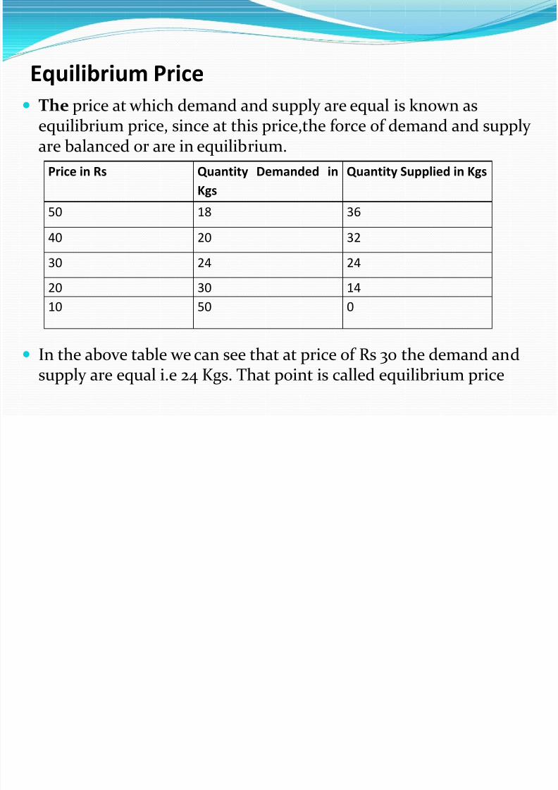
Equilibrium Price

The price at which demand and supply are equal is known asequilibrium price, since at this price,the force of demand and supply are balanced or are in equilibrium.

In the above table we can see that at price of Rs 30 the demand andsupply are equal i.e 24 Kgs. That point is called equilibrium price

Price in Rs Quantity Demanded in

Kgs

Quantity Supplied in Kgs

50 18 36

40 20 32

30 24 24

20 30 14

10 50 0

7/28/2019 IEM UNIT 2


Equilibrium Price

Demand Supply

Price Equilibrium Price P

Quantity Demanded or Supplied

At equilibrium price P demand and supply curve intersect and are equal.

7/28/2019 IEM UNIT 2


7/28/2019 IEM UNIT 2


Law of Diminishing Marginal Utility

Law of Diminishing Marginal Utility-Dr Marshall statesthat “other things being equal the additional benefit which aperson derives from a given increase of his stock of anythingdiminishes with the growth of the stock he has.”

In simple words-Other things being equal as we go on

consuming a commodity, the satisfaction derived from it’ssuccessive units goes on decreasing.

For eg A man who is hungry wants to eat chapatis. When heate 1st chapati that gave him maximum satisfaction(utility).But

as he ate additional chapattis the additional satisfaction,benefit or utility goes on decreasing. As he continues to eatfurther at a certain point the additional chapatti instead of giving satisfaction, it caused dissatisfaction or negative utility.This is expressed in table and graphical form –

7/28/2019 IEM UNIT 2



Chapatis Marginal Utility Total Utility

0 0 0

1 30 30

2 25 55

3 15 70

4 10 80

5 0 80

6 -5 75

7 -15 60

8 -25 45

7/28/2019 IEM UNIT 2


7/28/2019 IEM UNIT 2



Total

Utility

No of Chapatis

7/28/2019 IEM UNIT 2


7/28/2019 IEM UNIT 2


Consumer Surplus

The idea of Consumer Surplus was understood by a French engineer-economist , Arsene Jules Dupuit in 1844. But his explanation lackedscientific touch. Dr Alfred Marshall developed it further in hisPrinciples of Economics and named it as Consumer Surplus.

There are several things in our daily expenditure we find that the price we pay for a commodity is usually less than satisfaction (utility) which we obtain from that commodity. For example a packet of salt, a matchbox, a post card, a newspaper etc. These things have a high utility but arecheap and we are prepared to pay much more for them than what we areactually paying, if need arises.

Thus Consumer Surplus may be defined as the excess of utility (orsatisfaction) obtained by the consumer. It is measured by the differencebetween what we are prepared to pay and what we actually pay.

Consumer Surplus= What one is prepared to pay- What one actually pays.

Consumer Surplus= Total Utility obtained- Total amount spent. In Dr Marshall’s words “ The excess of the price which a consumer would

be willing to pay rather than go without the thing, over that which heactually does pay “

7/28/2019 IEM UNIT 2


Consumer Surplus

Consumer Surplus= Total utility-Total price paid =Area OMBQ- Area OPBQ = Area PMB

= Area PMB

M

Price

P B

O Q N

Quantity

Consumer Surplus

7/28/2019 IEM UNIT 2


7/28/2019 IEM UNIT 2


Consumer Surplus

Criticism/Limitations Hypothetical-The concept of consumer surplus is not real but imaginary. Difficult to measure utility- Since utility is in the mind of the consumer, it is

difficult measure consumer surplus. Very few consumer can tell us what exactly they are prepared to pay. Again different individual will be ready to differentprices for the same commodity.

Utilities are interdependent- The assumption that utility of a commodity

depends upon the quantity of commodity alone has been severally criticized,Because for example the utility of coffee not only depends on quantity of coffeebut also on supply and demand of its related goods like tea.

Difficult to group substitutes- Critics point out that there is hardly any commodity which has no substitute of it. And it is not possible to group the various substitutes as one.

The concept of consumer surplus cannot be applied to essential and may

prestigious goods. For example an affluent person dying of hunger may be willing to pay Rs 10000 for a piece of bread while he may be required to pay only Rs 10. As such, his consumer’s surplus will be equal to Rs 9990 which seemsridiculous. In case of prestigious goods e.g. rare paintings , diamonds etc what abuyer is generally willing to pay equals what he actually pays. It means there is noconsumer surplus. The concept of consumer surplus is thus illusory in somecases

7/28/2019 IEM UNIT 2


7/28/2019 IEM UNIT 2


Indifference Curve

Indifference Schedule- This is a schedule of various combinations of twocommodities Mango & Oranges. The consumer will find all combinationsequally satisfying.

In the above example in combination A the consumer has 25 mangoes and 5oranges. In the combination B he substitutes 10 mangoes with 2 oranges andso his Marginal rate of substitution is -5.0 In the combination C he substitutes5 mangoes with 5 oranges S0 MRS is -1.0. In the combination D he substitutes 4

mangoes with 8 oranges . So MRS is -0.5. In the combination E he substitutes 2mangoes with 10 oranges. So MRS is -0.2. Thus the consumer is willing to forgoless and less of Mangoes for obtaining more of oranges to keep his satisfactionsame.

Combination Mango (Y) Orange (X) Marginal Rate or Substitution (MRS)

A 25 5 0

B 15 7 25-15/5-7 = -5.0

C 10 12 15-10/7-12= -1.0

D 6 20 10-6/12-20= -0.5

E 4 30 6-4/20-30= -0.2

7/28/2019 IEM UNIT 2


Consumer Surplus

Mangoes

Oranges Indifference Curve

7/28/2019 IEM UNIT 2


Indifference Curve

Marginal Rate of Substitution- The rate at which aconsumer is willing to exchange successive units of acommodity with another will be marginal rate of substitution. It can be expressed as follows-

MRS= ∆Y/∆X = MUx/MUy= Slope of IndifferenceCurve.

One of the important condition for Indifference Curveis MRS diminishes. i.e. The consumer is willing to

forgo less and less of one commodity for obtainingmore of other to keep his satisfaction same,

7/28/2019 IEM UNIT 2


Characteristics of Indifference Curve 1.The Indifference curves always slopes negatively or downwards from

left to right.

The following indifference curves in which the slope is positive orconstant is not possible

Mangoes Mangoes

Oranges Oranges Mangoes

Oranges

7/28/2019 IEM UNIT 2


Characteristics of Indifference Curve

2. The indifference curve are convex to the origin of axes. The following indifference curve in which it concave to

the origin is not possible.

Oranges

Mangoes

7/28/2019 IEM UNIT 2


Characteristics of Indifference Curves

Mangoes


3.No Indifference Curves can intersect each other.

This above figure is not possible

7/28/2019 IEM UNIT 2


Characteristics of Indifference Curves

Mangoes IC1 IC2 IC3


4. Upper indifference curve indicate a higher level of satisfaction than lower level.

7/28/2019 IEM UNIT 2


Exceptions of Indifference Curve 1.Perfect Substitutes- In case of perfect substitutes the indifference

curve will be straight line with negative slope. In case of perfectsubstitutes like tea and coffee one cup for tea will be substitute for onecup of coffee and 5 cups of tea will be substitute for 5 cups of tea. SoMRS will not be diminishing and in fact it will be equal.

Tea

Coffee

7/28/2019 IEM UNIT 2


Characteristics of Indifference Curve 2. Complementary Commodity-

When 2 commodities are complementary to each other for example theright and left shoes or gloves a person cannot get satisfaction if he getsmore of one unit of such commodities. He will not give up one unit of commodity to get one more unit of other commodity. ThereforeMarginal Rate of Substitution will be zero and the indifference curve

will be 2 straight lines each running parallel to one of the axes andmeet each other vertically.

Shoe of Right Leg

Shoe of Left Leg

7/28/2019 IEM UNIT 2


Budget Line

Suppose a consumer has Rs 400 and cost of eachmango is Rs 8 and cost of each orange is Rs 4 he canbuy above combinations of mangoes and oranges.

No of Mangoes(Y) No of Oranges (X) Price of Mangoes Price of Oranges Total PrIce

50 0 400 0 400

40 20 320 80 400

30 40 240 160 400

20 60 160 240 400

10 80 80 320 400

0 100 0 400 400

7/28/2019 IEM UNIT 2


Budget Line

With the help of the indifference curve analysis we can explain the various combination of the 2 commodities a consumer can have which yield him equal satisfaction. But a consumer has limited income andthis is crucial in deciding the actual combination he can afford.

Mangoes

Budget Line for Income Rs 400

Budget Line for Income 600

Budget Line for Income Rs 300

Oranges

7/28/2019 IEM UNIT 2


Budget Line

A consumer’s income decides the position of the budgetline or price line. If the consumer can spent higher incomethan Rs 400 the budget line will shift upwards and if theconsumer’s income lowers then the budget line will shiftdownwards.

The prices of the commodities in this case the price of mangoes and oranges decide the slope of Price Line orBudget line.

Slope of Budget Line= Price of Mangoes (Y)/ Price of

Oranges (X) Thus the price line or Budget line shows the various

opportunities open to the consumer in the market with hisincome and the prices of two commodities.

7/28/2019 IEM UNIT 2


Consumer Equilibrium The indifference map represents the possible combinations of 2substitute commodities which give him equal satisfaction. Thebudget line or price line represents the possible combinations of 2 substitute commodities a consumer can have within his limitedincome. Thus consumer’s equilibrium can be revealed by usingindifference map and budget line.

This can be explained in following manner.

Suppose following is the indifference map of a consumerconsisting of indifference curves IC1, IC2, IC3 & IC4 for 2commodities mangoes and oranges. Suppose consumer has Rs400 as his income which he can spent on mangoes and orangesand cost of each mango is Rs 8 and Rs 4. AB is the price line orbudget line indicates the combinations of mangoes and orangeshe can have with this income of Rs 400 .

7/28/2019 IEM UNIT 2


Consumer Equilibrium

A P S

Mangoes U Q IC3 IC4

IC2

V IC1 R (Point of Equilibrium)

O X Y Z Oranges B

7/28/2019 IEM UNIT 2


Consumer Equilibrium Now we can find out the consumer equilibrium i.e. thespecific combination of mangoes and oranges which willgive him maximum satisfaction with his income of Rs400.He can choose any combination on Budget Line AB.

But he will select only point R at which Budget line istangent to Indifference curve IC3. as this point yield himmaximum satisfaction. Both budget line and IC3 haveequal slope at this point R. At this point he can have OV mangoes and OZ oranges. This is his point of maximum

satisfaction within his budget. This point R is his point of equilibrium. He will not choose any point on IC1 & IC2 asthey yield him less satisfaction. Even point S on IC3 or any point on IC4 will not chosen as this is beyond his budgetor income.

7/28/2019 IEM UNIT 2


Production Concepts

Input- An input is a good or service that is used intoprocess of production. Thus an input is anything which thefirm buys for use in its production or other process. For e.g.Labor, Capital, Land, raw materials and time.

Types of Input

Fixed Input- A fixed input is one whose quantity remainsfixed or constant for a certain level of output. It remainsfixed or inelastic in short run. For e.g. plant, building andmachinery.

Variable Input- A variable input is one whose quantity changes with output. It is variable or elastic in short run.For e.g. labor and raw materials.

Output- An output is any good or service that comes out of production process

7/28/2019 IEM UNIT 2


7/28/2019 IEM UNIT 2


Production Function

Q= F(Ld, L, K, M, T) Q- Output Ld- Land employed in production K-Capital employed in production (Machines, tools, raw

materials, fuel and consumables, money)

M- Management employed in production T-Technology employed in production. An increase in any of these factors of production when the otherfactors are constant will lead to increase in output.Generally the output of any commodity is related to inputs.Though the determinants may be almost the same, their relativeimportance varies from commodity to commodity. For egProduction of mobile phones requires larger capital andtechnology plays more crucial role in it than compared to a ballpoint pen. Similarly a diamond polishing process may requirelarger capital but smaller land as compared to a marble plishingprocess.

7/28/2019 IEM UNIT 2


Production Function

The concept of production function can be betterunderstood by considering 2 inputs for an output. Hey Although any 2 inputs can be considered we take laborand capital since they are most important variables of

all. Q= F( L, K)

7/28/2019 IEM UNIT 2


Production Function Short run refers to period of time in which supply of certain inputs (plant,

buildings and machines etc) is fixed or inelastic. In short run the productionof commodity can be increased by increasing the use of variable inputs likelabor and raw materials.

It is worth noting that short run does not refer to any fixed time period. Whilein some industries it may be matter of weeks or a few months, in some others(eg electric and power industry) it may be 3 or more years.

Long run refers to a period of time in which the supply of all inputs whether

fixed or variable can be increased to increase the production. Here only technology will not change. Thus in the short run the firm can increase its production by increasing only

labor since supply of capital is fixed. In the long run the firm can employ moreof both labor and capital. Accordingly the firm will have 2 types of productionfunctions. The Short run production function or single variable productionfunction given by

Q= f(L) In the Long run production function both Capital & Labor are included and it

is denoted by Q =f(K, L)

L f R V i bl P i P d i i h

7/28/2019 IEM UNIT 2


Law of Return to Variable Proportions- Production with one

variable input/ Law of Diminishing returns.

In short run the firms can employ only a limited orfixed quantity of fixed factors and an unlimitedquantity of variable factor.

It means that firm can employ in short run, varyingquantities of variable inputs against a given quantity of

fixed factors. This kind of change in input proportions leads to

variation in factor proportions.

The laws which bring out the relationship between

varying factor proportions and output are known aslaw of variable proportions or Law of Diminishingreturns or Law of returns to factor.

L f R V i bl P i P d i i h

7/28/2019 IEM UNIT 2



variable input/ Law of Diminishing returns.The law of Diminishing Returns states that if more and more

units of a variable input are applied to a given quantity of fixedinputs, the total output may initially increase at an increasingrate, but beyond a certain level, output increases at diminishingrate.

This means that marginal increase in total output or marginal

output decreases when additional units of variable factors areapplied to a given quantity of the fixed factors.

The main reason behind the operation of this law is thedecreasing labor-capital ratio. Given the quantity of fixed factor(capital) with increasing variable input (labor) capital-labor ratio

goes on decreasing. Thus each additional worker has less toolsand equipments to work. Consequently productivity of marginal

worker eventually decreases. As a result output increases but at adiminishing rates and beyond a point it will come down.

7/28/2019 IEM UNIT 2


L f R t t V i bl P ti P d ti ith

7/28/2019 IEM UNIT 2



variable input/ Law of Diminishing returns. In the example below the capital (K) is held constant at 10 units and labor (L) is

increased from 1 to 10 units, the output increases from 30 to 130 units atincreasing rate for increase of labor from 1 to 3 then output increases from 185to 300 for increase in labor from 4 to 9 at diminishing rate and when labor isincreased to 10 units the output falls down from 300 units to 280 units insteadof rising.

Labor Output TotalProduct(TP)

MarginalProduct(MP)

AverageProduct

Stage

1 30 30 0 30

2 70 70 40 35 1

3 130 130 60 43.33

4 185 185 55 46.25

5 225 225 40 45

6 260 260 35 43.33 2

7 285 285 25 40.71

L f R t t V i bl P ti P d ti ith

7/28/2019 IEM UNIT 2



variable input/ Law of Diminishing returns.

TP/MP/AP TP

AP

Labor MP

7/28/2019 IEM UNIT 2


7/28/2019 IEM UNIT 2


Return to Scale

Returns of Scale can be of 3 types-

Increasing Returns to Scale- Returns to scale are said tobe increasing if there is more than proportionate increasein output when compared to increase in inputs.

For eg if by employing 1 unit of labor and 1 unit of capital

you were getting 1 unit of out put and now if you increaselabor to 2 units and capital to 2 units and if you get morethan 2 units of output then this is increasing returns toscale.

If you increase labor and capital by 20 % and the outputincreases by more than 20 % then this is called asincreasing returns to scale.

This happens as the internal and external economies aremore than internal and external diseconomies.

7/28/2019 IEM UNIT 2


Return to Scale

Returns of Scale can be of 3 types- Constant Returns to Scale- Returns to scale are said to be

constant if the output increases in same proportion asthe increase in inputs.

For eg if by employing 1 unit of labor and 1 unit of capital you were getting 1 unit of out put and now if you increaselabor to 2 units and capital to 2 units and you get exactly 2units of output then this is constant returns to scale.

If you increase labor and capital by 20 % and the outputincreases by eaxctly 20 % then this is called as constantreturns to scale.

This happens due to balancing of internal and externaleconomies and internal and external diseconomies.

7/28/2019 IEM UNIT 2


Return to Scale

Returns of Scale can be of 3 types-

Decreasing Returns to Scale- Returns to scale are said tobe decreasing if the output increases in smallerproportion than the increase in inputs.

For eg if by employing 1 unit of labor and 1 unit of capital

you were getting 1 unit of out put and now if you increaselabor to 2 units and capital to 2 units and if you get lessthan 2 units of output then this is decreasing returns toscale.

If you increase labor and capital by 20 % and the outputincreases by less than 20 % then this is called as decreasingreturns to scale.

This happens as the internal and external economies areless than the internal and external diseconomies.

7/28/2019 IEM UNIT 2


Law of Return to Scale

If we increase the inputs by same proportion then output increases at

increasing rate i.e. increasing returns to scale, if we further increase theinput then the output increases at constant rate or same rate i.e.constant returns to scale and if we increase it further then outputincreases at decreasing rate i.e. decreasing returns to scale andultimately it declines. Thus marginal output 1st increases, thenbecomes constant and finally declines.

Marginal Output

Scale of Production

7/28/2019 IEM UNIT 2


Economies of Scale

They are classified as Internal or real economies of scale. External or pecuniary economies of scale. Internal or real economies of scale- These are those which arise from expansion of the plant size of the

firm. The economies are internal in the sense that economies are

internalized to the expanding firms and not available to non expandingfirms.Internal economies can be classified under following categories-

Economies in production/ Technical Economies. Economies in marketing Managerial Economies Financial Economies Managerial Economies Economies in transport and storage. Risk bearing economies

7/28/2019 IEM UNIT 2


Economies of Scale Economies in production/ Technical Economies-

These economies are the result of using better techniques of production facilitated by growth of firm. They are of 4 types-

• Economies of Increased dimension- These are economies of large size of amachine or plant or any other form of capital asset. For eg it is less costly to use adouble decker bus than to use to 2 buses. Also when dimensions of a rectangular water tank are doubled i.e. length, breadth and depth it’s capacity to hold waterincreases 8 times. One operator can run a small machine as well large machine so

large machine would reduce per unit labor cost.• Economies of Linking processes- Production involves several processes and

linking these processes the firm can achieve cost reduction. For eg production of cloth in textile mill may comprise such plants as 1. Spinning 2. Weaving 3. Printingand Pressing 4. Packing. Under the small scale of production the firm may not findeconomical to have all the plants.

• Economies of Superior techniques- Large scale production make it possible for a

firm to use advanced and more sophisticated machines. A large farm can use tractorinstead of wooden plough.• Economies of Specialization and Division of Labor-Difficult or risky operations

can be mechanized and those operations requiring individual care can be left tomanual work. Every job can be spilt in parts for division of labor and jobs can beassigned as per required skills. This saves unnecessary wastes of time and energy. Thisincreases efficiency and lowers cost

7/28/2019 IEM UNIT 2


7/28/2019 IEM UNIT 2


Economies of Scale

•

Financial Economies- Large firms can raise share capitalin large quantities because they can have a reputation, theshares listed on major stock exchanges and a wide marketfor their shares, bonds and debentures. They also enjoy better credit facilities from banks and preferential

treatment.• Risk bearing economies- Production involves certain

risks which are not insurable. A big firm can minimizethese risks in a number of ways. Firstly they can diversify i.e. produce various commodities satisfying different wants

of people. Such a diversification protects the firm fromcrisis in some fields. For e.g. ITC produces FMCG products,Cigarettes, Paper, Notebooks etc. So if heavy taxes arelevied on tobacco products it will not suffer a set back.

7/28/2019 IEM UNIT 2


Economies of Scale

Economies in transport and storage- It arises fromfuller utilization of transport and storage facilities.Transportation costs and storage costs are incurred onboth raw materials and finished products . The large

firms can own their own fleet of vehicles and buildtheir own storage facilities. This reduces bothtransport and storage costs. Besides own transportfacilities prevent the delays in transporting goods.

Some large scale firms like Bombay Port Trust havetheir own railway track from nearest railway point tothe factory or oil companies have their own fleet of tankers.

7/28/2019 IEM UNIT 2


Economies of Scale

External Economies- Industrial developmentinvolves two distinct aspects one growth of eachindividual firm and two industrialization of selectedareas, regions or belts through concentration of

different types of industries. The term externaleconomies was generally used to describe thoseeconomies which accrue to each member firm when whole industry expands. But in modern times this is

applicable to firms belonging to different industriesbut geographically located together. They are calledexternal because they do not flow from within the firmbut from outside.

7/28/2019 IEM UNIT 2


Economies of Scale

They are of following types- Economies of Concentration- When several firms of same industry or

different industries get localized at a place several advantages like skilled workers, facilities for transport, banks, hospitals for workers, schools for theirchildren, technical training institute for workers, roads and water supply getavailable. For eg textile mills have concentrated in cities like Mumbai, Ahmedabad, Surat, Solapur. Diamond cutting and polishing industry hasflourished in Surat, a huge industrial belt has developed in Ankleshwar, Pimpri

Chinchwad. Economies of Information- Publications like trade and research journals,

central research institutes, seminars and training programmes and suchactivities which are beyond the capacity of a single firm can be undertaken jointly. Many such activities are possible with the help of the Governmentinstitutions like universities and research laboratories.

Economies of Disintegration- When an industry grows in an area around acity some of the work or process can split up and handed over or outsourced tospecialized industries, institutions and agencies. When a large number of bookpublishers exist in an area specialized services of related experts like artist,designers, proof readers and printers become available to all publishers.

7/28/2019 IEM UNIT 2


Diseconomies of Scale

Large scale may encounter certain diseconomies and disadvantages.They are of 2 types.

Internal Diseconomies- They are internalized and they may be dueto following reasons-

Managerial Inefficiency- With fast expansion of the production scale,personal contacts and communication between owners and managersand managers and labor get rapidly reduced. Close control and

supervision is replaced by remote control. With increase in number of personnel decision making is complex , delayed and there arecoordination problems.

Labor inefficiency- Increase in number of workers encouragesunionization of labor and these results in strikes and lock outs. Thiscause stoppage of work and loss of output.

No direct contact with customers is possible. So tastes of consumers areignored. Products are standardized and no specialized services toconsumers are possible.

Large Scale production may cause over production and this may resultin losses.

7/28/2019 IEM UNIT 2


Diseconomies of Scale

External Diseconomies- These are the disadvantages which originatefrom outside the firm.

• Expansion of a particular industry causes certain diseconomies likecompetition among firms to secure raw materials and other resourcesfor itself causes prices to rise.

• Also with increase in demand for resources additional resources whichare available are naturally of lower quality as compared to those

already employed. For eg the best workers are selected first and if ore workers are required a firm has to appoint whosoever are availablerather than who are suited for the work. Thus not only wage rateincreases but productivity also goes down.

• Similar diseconomies flow from concentration of industries in certainlocalities. Overcrowding of cities, traffic congestion, pollution of air

and water, strain on civic amenities like drinking water, public health,sanitation and problems of housing, education, medical care and lawand order are some of the consequences. These affect efficiency of labor, availability of quick transport, timely deliveries of finishedproducts and overall strain on whole industrial system.

7/28/2019 IEM UNIT 2


7/28/2019 IEM UNIT 2


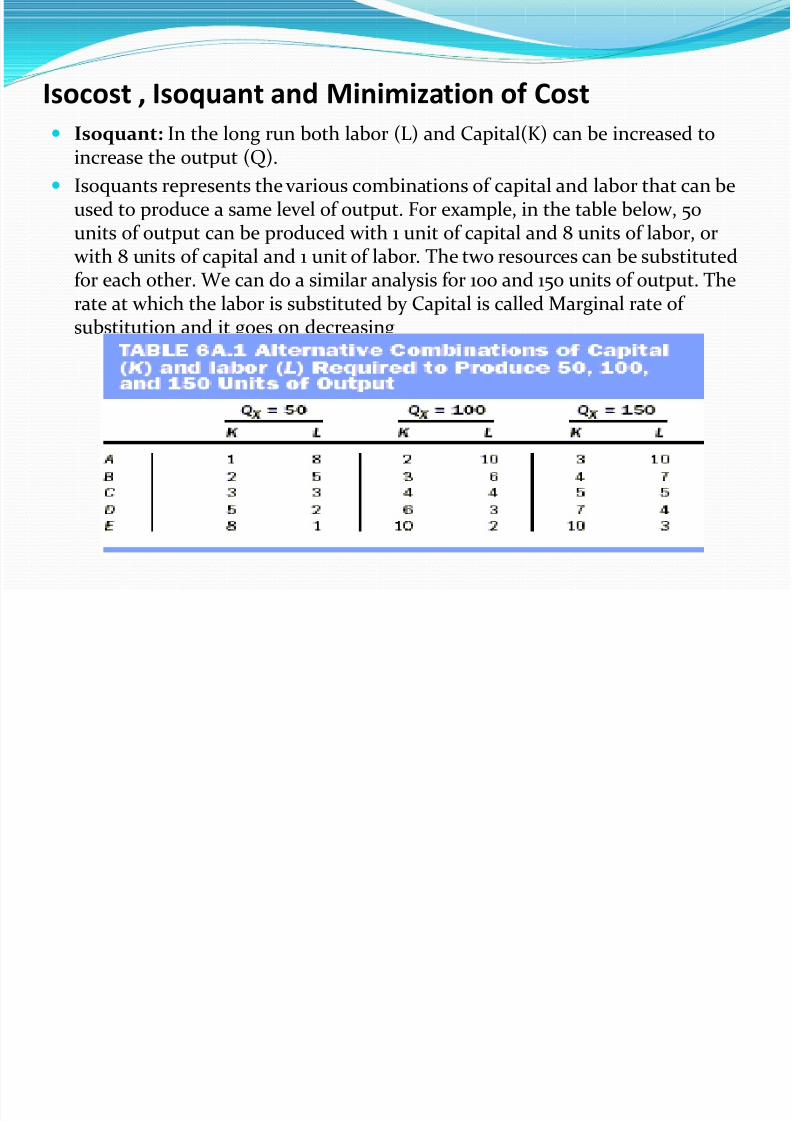
Isocost , Isoquant and Minimization of Cost

7/28/2019 IEM UNIT 2


Isoquant ,Isocost ,and Minimization of Cost

Marginal Rate of Substitution: The rate at which the labor is

substituted by Capital is called Marginal rate of substitution and it goeson decreasing, This is the slope of the Isoquant and it is ratio of Marginal product of Labor and Marginal Product of Capital .

7/28/2019 IEM UNIT 2



Characteristics of Isoquants- 1.The Isoquant curves always slopes negatively or

downwards from left to right.

2. The Isoquants are always convex to the origin of

axes. 3. No 2 Isoquant curves intersect each other.

4.Upper Isoquant curve represent a higher level of

production or output than lower Isoquant curve.

7/28/2019 IEM UNIT 2



Isocost Line-Firms need to know what it costs them to produce a level

of output. The isocost line allows us to represent the quantities of laborand capital that can be purchased at given input prices, given anamount of total cost or firms budget.

For eg If the budget of the firm towards total cost is Rs 400 and the costof Capital is Rs 8 and cost of Labor is Rs 4 then various combinations of

Labor and Capital are possible within the total cost of Rs 400.Units of Capital

Units of Labor

Cost of Capital

Cost of Labor

TotalCost

50 0 400 0 400

40 20 320 80 400

30 40 240 160 400

20 60 160 240 400

10 80 80 320 400

0 100 0 400 400

7/28/2019 IEM UNIT 2



Capital Iso Cost Line for Total Cost=400 Rs

Labor

Slope of Isocost Line= Price of Capital/Price of Labor

7/28/2019 IEM UNIT 2



A firms total cost or budget decides the position of theIsocost line. If the firm can spent higher total cost than Rs400 then Isocost line will shift upwards and if the firmsbudget/total cost lowers then the Isocost line will shiftdownwards.

The ratio of prices of the inputs in this case the price of capital and price of labor decide the slope of Isocost line.

Slope of Isocost Line= Price of Capital (Y)/ Price of Labor(X)

Thus the Isocost line shows the various opportunities opento the producer in the market with his total cost/budgetand the prices of two inputs i.e. labor and Capital.

7/28/2019 IEM UNIT 2


Cost Minimization using Isoquant and Isocost The Isoquants represents the possible combinations of 2 inputsi.e. Labor and Capital which give a producer or manufacturerequal output. The Isocost line represents the possiblecombinations of 2 inputs i.e. labor and Capital a producer canhave for a particular total cost/budget he is willing to spent .

Thus cost minimization or least can be revealed by usingIsoquant and Isocost line.

This can be explained in following manner.

Suppose IQ1 is the Isoquant curve of a producer for producing100 units of a product. AB, CD, EF are various Isocost lines for

various budget/total cost of the producer i.e. 500 Rs, 400 Rs and300 Rs respectively. A higher Isocost line indicates higher totalcost budget than lower Isocost line. Now which will be the point(Combination of Labor and Capital) of least total cost if producer wants to produce 100 units of the product.

7/28/2019 IEM UNIT 2


7/28/2019 IEM UNIT 2


Cost Minimization using Isoquant and Isocost

A

Isocost for Budget-500 Rs

C p

Capital E IQ1 for 100 units of production or output

Isocost for Budget-400 Rs

R

Q

F D B

Labor Isocost Budget-300 Rs Least Cost /Cost Minimization

h f d

7/28/2019 IEM UNIT 2


Theory of Production Costs

Cost Concepts

Actual Costs- It refers to the cost actually incurred inmoney terms. Such costs are recorded in the books of account of the firm. Eg Cost incurred by the firm inpayment for labor, material, plant, building, machinery,equipments, travelling and transport.

Opportunity Costs- It is second best use of resources which is foregone for availing the gains from the best use of resources. For eg A businessman with his limited resourcescan start either a business of printing or a lathe workshop.The expected income from printing is Rs 20000 and lathe

workshop is Rs 15000. Obviously he will do printingbusiness as the expected income is more in printing thanlathe. In this case he has foregone the opportunity of nextbest business i.e. lathe workshop. Thus Rs 15000 is theopportunity cost in this case.

h f d i

7/28/2019 IEM UNIT 2



Fixed Costs- are those which remain fixed in volume for a

certain given output. They do not vary with variation inoutput between zero and certain level of output. For eg incase of textile plants producing 10 lakh metres of cloth per

year the costs on account of plant and machinery, building

will remain constant at all level of output from 1 metre to 1lakh metres. This costs are called as fixed costs.

Variable Costs- Variable costs are those which vary moreor less proportionately with the output are known as

variable cost. In the above example costs of raw materials,labor, electric power, running cost of fixed capital such asfuel, ordinary repairs, maintenance are variable costs.

Th f P d i C

7/28/2019 IEM UNIT 2



Short run costs- It can be defined as costs which vary with variation of output for certain level of output.Thus short run costs are same as variable costs.

Long run costs- These are the costs which areincurred on the fixed assets like plant, buildingmachinery, land and are not used in single batch of production but are used over entire period of time.They are by implication same as fixed costs.

Th f P d i C

7/28/2019 IEM UNIT 2



Cost Function- It is the relationship between Cost

and its determinants and is represented as follows-

C=f(Q, T, Pf, K)

C-Total Cost

Q-Quantity produced

Pf- factor price

K-Capital fixed factor.

Short Run Cost Function- In the short run all thedeterminants of cost other than output Q are constant.So the cost function function will bE

C=f(Q).

Th f P d ti C t

7/28/2019 IEM UNIT 2


Theory of Production Costs Relationship between Cost and Output in the Short Run: Total Cost(TC)- It is defined as the total cost incurred to produce a given quantity of

output. In short run total cost is composed of 2 major elements i.e. Total Fixed Cost(TFC) & Total Variable Cost(TVC).

TC= TFC + TVC TFC remains fixed in short run for a certain level of output and TVC varies with variation

in the output. Average Total Cost- It is obtained by dividing total cost (TC) by the quantity of output

produced (Q).

ATC=TC/Q Similarly AVC= TVC/Q AFC=TFC/Q Marginal Cost(MC)- It is the addition to the total cost on account of producing one

additional unit of product or it is cost of marginal units produced. MC=∆TC/∆Q

Since ∆TC=∆TFC+∆TVC In short run ∆TFC=0 Therefore ∆TC=0+∆TVC ∆TC=∆TVC MC= ∆TVC/∆Q

Th f P d ti C t

7/28/2019 IEM UNIT 2



Example:Q(units)

TFC TVC TC AFC AVC ATC MC

0 140 - 140 - - - -

10 140 70 210 14.0 7.0 21.0 7

20 140 110 250 7.0 5.5 12.5 4

30 140 180 320 4.7 6.0 10.7 7

40 140 280 420 3.5 7.0 10.5 10

50 140 450 590 2.8 9.0 11.8 17

60 140 720 860 2.3 12.0 14.3 2770 140 1120 1260 2.0 16.0 18.0 40

80 140 1680 1820 1.8 21.0 22.8 56

7/28/2019 IEM UNIT 2


Th f P d ti C t

7/28/2019 IEM UNIT 2



1.Average fixed cost (AFC) :

. AFC decreases throughout the output (Q) range. b. If we extend the output range further to the right, AFC

moves closer and closer to the horizontal axis (Q - axis).

c. WHY? AFC = TC / Q and AFC decreases as Q increases

2. Average variable costs (AVC) :

a. The average variable cost curve is U - shaped.

b. AVC first decreases, reaches a minimum, and theincreases.

c. WHY? Something you learned a little earlier known asthe LAW OF DIMINISHING RETURNS and the LAW OFINCREASING COSTS

Theor of Prod ction Costs

7/28/2019 IEM UNIT 2



3. Average total costs (ATC) :

a. ATC has similar shape of AVC. However, it fallsfaster than AVC in the beginning and rises slower afterreaching its minimum point.

b. WHY?

ATC = AFC + AVC AFC and AVC both fall in the beginning, at some point

however, AVC begins to rise while AFC continues tofall.

When the increase in AVC OUTWEIGHS the decreasein AFC, the ATC will begin to increase forming thefamiliar U - shaped curve


7/28/2019 IEM UNIT 2



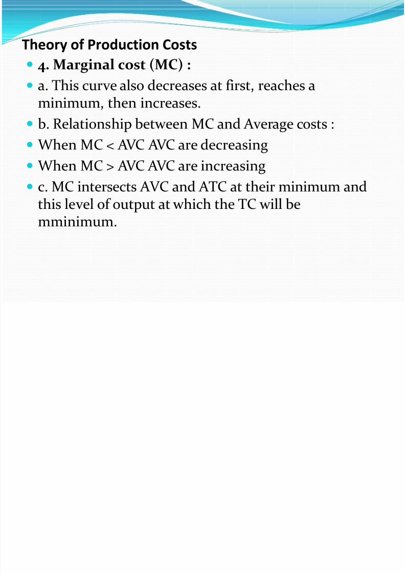
4. Marginal cost (MC) :

a. This curve also decreases at first, reaches aminimum, then increases.

b. Relationship between MC and Average costs :

When MC < AVC AVC are decreasing When MC > AVC AVC are increasing

c. MC intersects AVC and ATC at their minimum andthis level of output at which the TC will be

mminimum.

7/28/2019 IEM UNIT 2



iem unit 2

Documents