IEEE

Proo

f

IEEE TRANSACTIONS ON INTELLIGENT TRANSPORTATION SYSTEMS 1

Algebraic Connectivity Maximization for AirTransportation Networks

1

2

Peng Wei, Member, IEEE, Gregoire Spiers, and Dengfeng Sun, Member, IEEE3

Abstract—It is necessary to design a robust air transportation4network. An experiment based on the real air transportation5network is performed to show that algebraic connectivity is a fair6measure for network robustness under random failures. Therefor,7the goal of this paper is to maximize algebraic connectivity. Some8researchers solve the maximization of the algebraic connectivity9by choosing the weights for the edges in the graph. Others focus10on the best way to add edges in a network in order to optimize11the connectivity. In this paper, the authors formulate a new air12transportation network model and show that the corresponding13algebraic connectivity optimization problem is interesting because14the two subproblems of adding edges and choosing edge weights15cannot be treated separately. The new problem is formulated and16exactly solved in a small air transportation network case. The17authors also propose the approximation algorithm in order to18achieve better efficiency. For large networks, the semidefinite pro-19gramming with cluster decomposition is first presented. Moreover,20the algebraic connectivity maximization for directed networks21is discussed. Simulations are performed for a small-scale case,22large-scale problem, and directed network problem.23

Index Terms—Author, please supply index terms/keywords24for your paper. To download the IEEE Taxonomy go to http:25//www.ieee.org/documents/Taxonomy_v101.pdf.AQ1 26

I. INTRODUCTION27

AN AIR transportation network consists of distinct airports28

(cities) and direct flight routes between airport pairs [1].29

Usually, a graph G(V,E) is used to describe an air trans-30

portation network [2], [3], where the node set V represents all31

the n airports and the edge (link) set E represents all the m32

direct flight routes between airports. If a direct flight route from33

airport a to airport b exists, normally, the direct return route34

from airport b to airport a also exists [4]; G(V,E) is constructed35

as an undirected simple graph, where the airports are indexed36

as {vi|i = 1, 2, . . . , n} and the direct flight routes are named37

as eij if there is a direct route between airports vi and vj .38

There are many factors to be considered when designing an air39

transportation network, such as traffic demand, operating cost,40

airport hubs, market competition, multiairport systems, and41

Manuscript received November 6, 2012; revised April 5, 2013 andAugust 20, 2013; accepted October 1, 2013. The Associate Editor for this paperwas J.-P. B. Clarke.

P. Wei is with the Operations Research and Advanced Analytics, AmericanAirlines, Fort Worth, TX 76155 USA (e-mail: peng.wei@aa.com).

G. Spiers was with the Department of Applied Mathematics, École Polytech-nique, 91120 Palaiseau, France. He is now with Amadeus S.A.S., 06902 SophiaAntipolis, France (e-mail: gregoire.spiers@polytechnique.org).AQ2

D. Sun is with the School of Aeronautics and Astronautics, Purdue Univer-sity, West Lafayette, IN 47907 USA (e-mail: dsun@purdue.edu).

Color versions of one or more of the figures in this paper are available onlineat http://ieeexplore.ieee.org.

Digital Object Identifier 10.1109/TITS.2013.2284913

Fig. 1. Air transportation network route map for Virgin America Airlines.

scheduling [5]–[14]. In this paper, we focus on investigating 42

the network robustness maximization, particularly the algebraic 43

connectivity maximization. 44

A. Algebraic Connectivity and Air Transportation 45

Network Robustness 46

In order to illustrate the relationship between the algebraic 47

connectivity and air transportation network robustness, a real 48

air transportation network of Virgin America is studied. The 49

following experiment shows that algebraic connectivity is a 50

fair measurement for the network robustness with regard to 51

random link failures under the current Virgin America network 52

topology. 53

According to the current route map of Virgin America in 54

Fig. 1, we consider the 16 airports in the United States and 55

obtain the adjacency matrix as Table I. The 16 United States air- 56

ports include Boston (BOS), New York City/John F. Kennedy 57

(JFK), Philadelphia, Washington Dulles International Air- 58

port (DC/IAD), Ronald Reagan Washington National Airport 59

(DC/DCA), Chicago O’Hare International Airport (ORD), 60

Orlando, Fort Lauderdale, Dallas/Fort Worth, Seattle, Portland, 61

San Francisco, Los Angeles, Las Vegas, San Diego, and Palm 62

Springs and are indexed as numbers 1–16. San Francisco Inter- 63

national Airport (SFO) and Los Angeles International Airport 64

(LAX) are two major hubs of the entire network. Both have at 65

least one direct flight to almost all the other airports. 66

In order to show how well the algebraic connectivity can 67

measure the robustness of an air transportation network, we 68

1524-9050 © 2013 IEEE

IEEE

Proo

f

2 IEEE TRANSACTIONS ON INTELLIGENT TRANSPORTATION SYSTEMS

TABLE IADJACENCY MATRIX CONSISTS OF 16 VIRGIN AMERICA AIRLINES AIRPORTS IN THE USA

created six different weighted air transportation networks with69

the same topology in Table I by randomly assigning one of70

the three types of link weights to each route. Each link weight71

is an indication of link strength. A larger weight represents a72

stronger link and a smaller weight shows that the corresponding73

link is easier to fail. There are many reasons for route failure,74

such as weather disturbance, long ground delay program, long75

airspace flow program (AFP), aircraft mechanical problem, and76

upline flight delay/cancelation. The route failure rate statis-77

tics are published by each origin–destination pair (route) and78

different routes have different features [15]. For example, the79

route failure rate between JFK and BOS during summer is80

higher than that between SFO and LAX because of the crowded81

northeastern airspace (AFP is more frequent) and more summer82

thunderstorms. Another example is that a shorter route is easier83

to fail than a longer transcontinental route because: 1) airlines84

usually put larger aircraft on transcontinental route, and these85

aircraft are more robust to weather disturbance and 2) airlines86

are more likely to cancel shorter route flights because the flight87

frequency on a shorter route is higher; therefor, the passengers88

on the canceled flight are easier to protect (be reaccommodated89

to later flights). In summary, each route has its own features90

and thus in our model we consider that they have different91

possibilities for failure.92

The three types of link weights are mapped to different link93

failure probabilities (see Table II). The link failure probability94

range [%0, %5] is obtained from the historical flight cancelation95

rate between September 15, 2012, and November 15, 2012 [15].96

A network failure is defined as the existence of at least one97

pair of nodes that cannot access each other through any one or98

multiple links. For each one of the six weighted networks, 100099

trials are performed. In each trial, every link fails randomly100

TABLE IIMAPPING BETWEEN LINK WEIGHTS AND LINK FAILURE PROBABILITIES

TABLE IIINETWORK FAILURE NUMBERS WITH DIFFERENT ALGEBRAIC

CONNECTIVITY VALUES

according to the failure probabilities listed in Table II. The total 101

number of network failures is counted in 1000 random trials. 102

The results are shown in Table III with algebraic connectivity 103

sorted in ascending order. 104

We can see that with higher algebraic connectivity, the 105

network is more robust and has fewer network failures. With 106

lower weighted algebraic connectivity, the network is easier to 107

break down. Therefor, algebraic connectivity is a fair robustness 108

measure for the air transportation network, and we need to find 109

the maximized algebraic connectivity. 110

The air traffic demand is expected to continue its rapid 111

growth in the future. The Federal Aviation Administration 112

estimated that the number of passengers is projected to increase 113

by an average of 3% every year until 2025 [16]. The expanding 114

traffic demand on the current air transportation networks of 115

different airlines will cause more and more flight cancelations 116

with the limited airport and airspace capacities. As a result, 117

more robust air transportation networks are desired to sustain 118

IEEE

Proo

f

WEI et al.: ALGEBRAIC CONNECTIVITY MAXIMIZATION FOR AIR TRANSPORTATION NETWORKS 3

the increasing traffic demand for each airline and for the entire119

National Airspace System (NAS). This is the major motivation120

of this paper.121

B. Related Work122

An air transportation network and its robustness have been123

studied over the last several years. Guimera and Amaral first124

studied the scale-free graphical model of the air transportation125

network [1]. Conway showed that it was better to describe126

the national air transportation system or the commercial air127

carrier transportation network as a system of systems [17].128

Bonnefoy showed that the air transportation network was scale129

free with aggregating multiple airport nodes into meganodes130

[18]. Alexandrov defined that on-demand transportation net-131

works would require robustness in system performance [19].132

The robustness of an on-demand network would depend on the133

tolerance of the network to variability in temporal and spatial134

dynamics of weather, equipment, facility, crew positioning, etc.135

Kotegawa et al. surveyed different metrics for air transportation136

network robustness, including betweenness, degree, centrality,137

connectivity, etc. [20]. They selected clustering coefficient and138

eigenvector centrality as the network robustness metrics in139

their machine learning approach. Bigdeli et al. compared alge-140

braic connectivity, network criticality, average degree, average141

node betweenness, and other metrics [21]. Jamakovic et al.142

found that algebraic connectivity was an important metric in143

the analysis of various robustness problems in several typical144

network models [22], [23]. Byrne et al. showed that algebraic145

connectivity was the efficient measure for the robustness of146

both small and large networks [24]. Vargo et al. in [3] chose147

algebraic connectivity as the robustness metric and built the148

optimization problem solved by the edge swapping-based tabu149

search algorithm.150

In this paper, we measure the robustness of air transportation151

network by computing the algebraic connectivity, which is152

usually considered as one of the most reasonable and efficient153

evaluation methods [24], [25]. Although the maximized value154

of algebraic connectivity is abstract, the optimized air trans-155

portation network structure and weighting assignment provide156

us the applicable design.157

There are some literature on algebraic connectivity maxi-158

mization. The problems studied can be divided into two cat-159

egories, namely, the edge addition problem and the variable160

weights problem.161

1) Edge addition problem: The goal is to add or remove a162

given number of k edges on a graph in order to get the best163

algebraic connectivity. The edges to be added or removed164

are selected from a candidate set. The algorithms that165

have been developed to solve the problem include tabu166

search [25], greedy algorithms [25], [26], and rounded167

semidefinite programming (SDP) [26].168

2) Variable weights problem: The edges of the graph are169

fixed and the goal is to determine the edge weights in170

order to maximize the algebraic connectivity. This is171

a convex optimization problem that is often solved by172

using an SDP formulation [27]–[29] or a subgradient173

algorithm [30].174

C. Contribution 175

The major contribution of this paper compared with what 176

has been studied is that we find that, in order to maximize 177

the algebraic connectivity, the edge addition problem and the 178

variable weights problem cannot be studied separately. Solving 179

one of them independently will only result in a suboptimal 180

solution. Therefor, we propose a new algorithm to solve both 181

problems at the same time. How to choose the edges of the 182

graph is demonstrated, as well as how to assign their weights. 183

In addition, we are the first to present the cluster decomposition 184

method to achieve better computation efficiency for large-scale 185

networks. We are also the first to discuss the algebraic connec- 186

tivity maximization for directed air transportation networks. 187

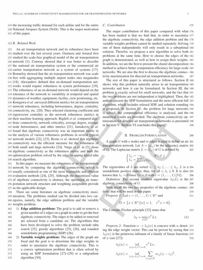
The rest of this paper is structured as follows. Section II 188

shows why this problem naturally arises in air transportation 189

networks and how it can be formulated. In Section III, the 190

problem is exactly solved for small networks, and the fact that 191

the two problems are not independent is highlighted. Then, the 192

authors present the SDP formulation and the more efficient full 193

algorithm, which includes relaxed SDP, and solution rounding 194

is proposed. In Section IV, the problem for large networks 195

is solved, the computational efficiency is analyzed, and the 196

numerical results are provided. The algebraic connectivity op- 197

timization for directed air transportation networks is presented 198

in Section V. Section VI concludes this paper. 199

II. PROBLEM FORMULATION 200

A graph G with n nodes and m edges is used to define an air 201

transportation network. Let A = (aij) be the adjacency matrix 202

of G. The Laplacian matrix L = (lij) of G is defined by 203{lij = −aij , if i �= jlii =

∑nj=1 aij .

The eigenvalues of L are sorted λ1 ≤ λ2 ≤ . . . ≤ λn. L is a 204

semidefinite positive matrix; thus, for all i, λi ≥ 0. It is also 205

known that λ1 = 0 since Le = 0 with e = (1, . . . , 1) [31]. 206

Definition: The second smallest eigenvalue λ2(L) is the 207

algebraic connectivity of G. 208

Now, recall the two key properties of the algebraic connec- 209

tivity that will be used in this paper. 210

Property 1: Let e = (1, . . . , 1) ∈ Rn and 211

Ω ={x ∈ R

n|‖x‖ = 1, eTx = 0}.

The Courant–Fischer principle [32] states that 212

λ2 = minx∈Ω

xTLx. (1)

Property 2: Function w → λ2(w) is concave with w denot- 213

ing the edge weight vector. This can be proven by seeing that 214

λ2(w) is the pointwise infimum of a family of linear functions 215

of w (see [27]) 216

λ2(w) = inf‖v‖=1,eT v=0

vTLv,

λ2(w) = inf‖v‖=1,eT v=0

∑(i,j)∈E

wij(vi − vj)2.

IEEE

Proo

f

4 IEEE TRANSACTIONS ON INTELLIGENT TRANSPORTATION SYSTEMS

The goal of this paper is to maximize the algebraic connec-217

tivity of the network under several constraints.218

There are m = (n(n− 1))/2 edges in the complete sym-219

metric graph. Each has a weight wij representing the link220

strength, as described in Section I. The following constraints221

are considered.222

The edge weight representing link strength must be within223

the range between the lower bound α and the upper bound β224

∀(i, j) ∈ E, α ≤ wij ≤ β.

When there is no edge connecting vi and vj , the corresponding225

wij = 0.226

There exists an operating cost cij for each link. In a real air227

transportation network, the cost for a route contains the fuel228

cost, aircraft maintenance cost, crew/flight attendant labor cost,229

cost for arrival/departure slots at runways, cost for gates at230

origin/destination airports, and cost for flying through airspace231

(international flights). In this paper, we use one link cost to232

represent the integrated operating cost. The operating cost is233

higher for a stronger link for several practical reasons. For234

example, we know that the most effective way to avoid a235

mechanical problem cancelation is to have spare parts or even236

a spare aircraft. Similarly, the most effective way to avoid a237

cancelation caused by crew legality or crew scheduling is to238

have enough standby crew. Both approaches can increase link239

strength; at the same time, they introduce higher costs. As for240

weather disturbances, to load extra fuel will give an aircraft241

more flight plan options with which it can be rerouted to avoid242

weather problems and prevent the cancelation. However, extra243

fuel also introduces higher cost. In addition, larger aircraft are244

more robust to weather disturbances. Nevertheless, to operate245

a larger aircraft costs more because of more fuel needed, more246

flight attendants, and even more crew (for international flights).247

Therefor, in this paper, we consider the linear cost for link248

strength. The total operating cost budget for all the links is249

limited by250 ∑ij

wijcij ≤ C.

In summary, the complete problem that the authors aim at251

solving is252

maxw

λ2 (L(w)) s.t.

{∑ij wijcij ≤ C

wij ∈ {0, [α, β]} . (P)

A. Alternative Formulation253

In order to be able to solve the problem, the authors need to254

reformulate it by adding decision variables. The idea is to add,255

for each edge (i, j), a binary variable xij stating if there exists256

an edge between vi and vj257

xij = 1 ⇔ wij �= 0.

This is useful since now the domain of w can be expressed as258

∀(i, j), αxij ≤ wij ≤ βxij .

The problem now becomes 259

maxx,w

λ2 (L(w)) s.t. :

⎧⎨⎩

xij ∈ {0, 1}∑ij wijcij ≤ C

αxij ≤ wij ≤ βxij .

Then, variable k is added, which determines the number of 260

edges in the graph. The final formulation of the problem is 261

maxx,w,k

λ2 (L(w)) s.t. :

⎧⎪⎨⎪⎩

∑i,j xij = k

xij ∈ {0, 1}∑i,j wijcij ≤ C

αxij ≤ wij ≤ βxij .

(2)

B. Difficulty 262

An important remark is that the problem cannot really be 263

split into two steps of first deciding whether w = 0 or not and 264

followed by choosing the appropriate weights. This is due to 265

the fact that there are lower bound and upper bound constraints 266

on w. However, assuming that the two steps are independent, a 267

decoupled approach can be tried first. The first step is to choose 268

edges for the empty graph that corresponds to the edge addition 269

problem introduced in [25] 270

maxx

λ2(L(x))

s.t. :∑i

xi = k, xi ∈ {0, 1},∑i

xici ≤C

α

and the second step is to choose the weights on them 271

maxw

λ2 (L(w))

s.t. :∑i

wici ≤ C, αyi ≤ wi ≤ βyi, y = xopt.

Later, it will be seen that, if this approach is used, the result will 272

not be optimal. 273

C. Relaxation 274

The relaxation (R) of the problem is obtained by allowing 275

noninteger values for x 276

∀(i, j) ∈ E, xij ∈ [0, 1].

This is the same as choosing w ∈ [0, β] without variables x 277

and k. However, these variables will be necessary in order to 278

be able to get the integer solution from this relaxed one. It is 279

noticed that the solution of (R) is a concave function of k. 280

D. Concavity in k 281

The first important property is that the solution of (R) is 282

concave in k, which will be used in the golden section search 283

algorithm in Algorithm 1. More precisely, Λ is defined such that 284

Λ(k) = maxx,w

λ2 (L(w)) s.t.

⎧⎪⎨⎪⎩

∑i xi = k

xi ∈ [0, 1]∑i wici ≤ C

αxi ≤ wi ≤ βxi.

IEEE

Proo

f

WEI et al.: ALGEBRAIC CONNECTIVITY MAXIMIZATION FOR AIR TRANSPORTATION NETWORKS 5

Property 3: Λ(k) is a concave function.285

This property is important since it shows that the maximiza-286

tion of the algebraic connectivity is related to the number of287

edges in the graph. By solving the problem for very few values288

of k, a good knowledge on kopt can be obtained.289

Proof: Consider k1 and k2 in R and γ ∈ [0, 1] such that290

Λ(ki) > 0 for i = 1, 2. The idea is to use the fact that w →291

λ2(L(w)) is concave (please see Property 2).292

Λ (γk1+(1−γ)k2)

=maxx,w

λ2 s.t.

⎧⎪⎨⎪⎩

∑i xi=γk1+(1−γ)k2

xi ∈ [0, 1]∑i wici≤C

αxi≤wi≤βxi

≥maxx,w

λ2 s.t.

⎧⎪⎪⎪⎪⎨⎪⎪⎪⎪⎩

∑i x

(1)i =k1,

∑i x

(2)i =k2

x(j)i ∈ [0, 1], j=1, 2

x=γx(1)+(1−γ)x(2)∑i wici≤C

αxi≤wi≤βxi

≥maxx,w

λ2 s.t.

⎧⎪⎪⎪⎪⎪⎨⎪⎪⎪⎪⎪⎩

∑i x

(1)i =k1,

∑i x

(2)i =k2

x(j)i ∈ [0, 1], j=1, 2

w=γw(1)+(1−γ)w(2)∑i wici≤C

αx(j)i ≤w

(j)i ≤βx

(j)i

≥γmaxx,w

λ2 s.t.

⎧⎪⎨⎪⎩

∑i xi=k1

xi ∈ [0, 1]∑i wici≤C

αxi≤wi≤βxi

+(1−γ)maxx,w

λ2 s.t.

⎧⎪⎨⎪⎩

∑i xi=k2

xi ∈ [0, 1]∑i wici≤C

αxi≤wi≤βxi

≥γΛ(k1)+(1−γ)Λ(k2)

which proves that Λ is concave in k. �293

III. SMALL-SCALE AIR TRANSPORTATION NETWORKS294

A. Exact Solution for Small Networks295

If all weights have to be chosen within an interval, the296

problem becomes a convex optimization problem and it can297

be solved using an SDP solver. The idea here is to try all the298

possible configurations for which all the weights are either 0299

or in [α, β]. Then, each configuration can be independently300

optimized and the one that leads to the best result can be found.301

Consider that n nodes are chosen randomly. There are m =302

(n(n− 1))/2 edges and 2m configurations to test. For each303

configuration, if Y is the set of the edges that are actually in304

the graph, the following problem needs to be solved:305

maxw

λ2 (L(w)) s.t.

⎧⎨⎩

∑ij wijcij ≤ C

α ≤ wij ≤ β, ∀(i, j) ∈ Ywij = 0, ∀(i, j) /∈ Y .

Fig. 2. Results of (k, λ2) for all the configurations of n = 5 and C = 6.5.

Fig. 3. Results of (k, λ2) for all the configurations of n = 6 and C = 8.

This can be done by solving the SDP corresponding to the 306

weight optimization problem (see [27] for details) 307

minw

∑i

wici s.t.

⎧⎨⎩

α ≤ wi ≤ β, ∀(i, j) ∈ Ywij = 0, ∀(i, j) /∈ YL(w) I − 1

neeT .

It becomes impossible to exactly solve the problem when n is 308

large. Therefor, the authors assume n to be small in this section. 309

1) Small-Scale Exact Solution Results: For each configura- 310

tion, the number of edges k in the graph is computed. The 311

results of (k, λ2) are plotted in Figs. 2 and 3 for two different 312

networks. 313

It is noticed that the best connectivity is not reached at the 314

maximum number of edges; therefor, the choice of the edges 315

and the choice of the weights are not independent. 316

It is also noticed that, unlike the continuous case, the discrete 317

shape given by k → Λ(k) in Figs. 2 and 3 is not exactly con- 318

cave. However, it has almost the shape of a concave function; 319

hence, the authors will be able to consider it concave in the 320

approximate case later on. 321

IEEE

Proo

f

6 IEEE TRANSACTIONS ON INTELLIGENT TRANSPORTATION SYSTEMS

Fig. 4. Optimal network for n = 5 with the weights. p = 0, α = 2, andC = 6.5.

The exact solution for a network of size n = 5 is shown322

in Fig. 4. As it is impossible to exactly solve this problem323

for networks with a larger size, an algorithm is going to be324

designed, which solves it approximately. The main idea is to325

use the quasi-concave shape of function Λ(k).326

For the practical problem with a larger size, the first step is to327

choose a value for k. The authors are able to solve the relaxed328

version (R) of the problem where x is a noninteger variable.329

Then, the result can be rounded to obtain a feasible solution for330

the original problem (P ).331

2) Maximum Number of Edges: Because of the minimum332

value α for the weights, there exists a limit in the number333

of edges in the graph. Here, the maximal number of edges334

klim needs to be found. Regardless of the performance of the335

network, edges are added until the operating cost constraint is336

reached. Consider that w = αx, which is the minimum weight,337

and the problem is to solve a trivial form of the knapsack338

problem339

maxx∈{0,1}

∑i

xi

s.t.∑i

xici ≤C

α.

Indeed, if klim is the solution of this problem, it can be guaran-340

teed that there will not be any solution of k > klim.341

When the cost ci is sorted by increasing order, it can be342

obtained that343

klim∑s=1

cs ≈C

α

which, for large-enough n, can be approximated by the follow-344

ing formula:345

klim∫1

g(s)ds =C

α

Fig. 5. Function g for random points in [0, 1]2.

Fig. 6. C as a function of klim with the quadratic fitting.

where 346

∀s ∈ [1, klim], g(s) = c�s .

If the n nodes are randomly chosen in a square, function g 347

is very close to a linear function (except at the very beginning 348

and at the very end). This can be verified in Fig. 5. Using this 349

information, it can be obtained that 350

a2k2lim + a1klim + a0 =

C

α(3)

where a0, a1, and a2 are constant parameters. Finally 351

klim =−a1 +

√a12 − 4a2

(a0 − C

α

)2a2

. (4)

It is shown in Fig. 6 that the quadratic result obtained by (4) 352

is a very good approximation. 353

IEEE

Proo

f

WEI et al.: ALGEBRAIC CONNECTIVITY MAXIMIZATION FOR AIR TRANSPORTATION NETWORKS 7

B. SDP Formulation354

To solve the larger size problem, the relaxation of the prob-355

lem is expressed as an SDP that will be solved efficiently. When356

v is not normalized, recall (1) in Property 1, which can be then357

transformed as358 {λ2 = maxλ λλvT v ≤ vTLv∀v ∈ R

n, vT e = 0.

Variable μ is added, which allows any v ∈ Rn359 {

λ2 = maxλ,μ λ∀v ∈ R

n, vT (μeeT )v + vTLv − λvT v ≥ 0.

It can be written using Loewner’s order [33]360 {λ2 = maxλ,μ λμeeT + L− λI 0.

(5)

The relaxation of the problem that needs to be solved is361

maxx,w,k

λ2 (L(w)) s.t.

⎧⎪⎨⎪⎩

∑i xi = k

xi ∈ [0, 1]∑i wici ≤ C

αxi ≤ wi ≤ βxi

which now becomes with (5)362

maxx,w,k,λ,μ

λ s.t.

⎧⎪⎪⎪⎨⎪⎪⎪⎩

∑i xi = k

xi ∈ [0, 1]∑i wici ≤ C

αxi ≤ wi ≤ βxi

μeeT + L− λI 0.

(6)

This problem is an SDP since there is a semidefinite constraint363

and all the other constraints are linear. It can be solved effi-364

ciently by an SDP solver. SeDuMi [34] is used in this paper.365

1) Optimality Conditions: The primal SDP is366

maxx,w,k,λ,μ

λ s.t.

⎧⎪⎪⎪⎨⎪⎪⎪⎩

∑i xi = k

xi ∈ [0, 1]∑i wici ≤ C

αxi ≤ wi ≤ βxi

μeeT + L− λI 0.

The variables are rescaled by dividing w, k, and x by λ and C.367

The dual SDP problem is368

minx,w,k,λ

∑i

wici s.t.

⎧⎪⎪⎨⎪⎪⎩

∑i xi = k

xi ∈ [0, 1]αxi ≤ wi ≤ βxi

L I − 1nJ

where J is the all-one matrix. When xij is relaxed (please see369

Section II-C), the relaxed dual SDP formulation is370

minx,w,k,λ

∑i

wici s.t.

{0 ≤ wi ≤ βL I − 1

nJ.

X is the matrix of the operating costs. The matrix format371

relaxed dual SDP is therefor372

maxX

⟨I − 1

nJ,X

⟩s.t.

{X 0〈E,X〉 = cij

where E is the matrix with Eii = Ejj = 1 and Eij=Eji=−1.373

Fig. 7. Upper bound: λ2 = f(k).

The Karush–Kuhn–Tucker optimality conditions are 374⎧⎪⎨⎪⎩

SX = XS = 0S 0, X 0〈E,X〉 = cijL− I + 1

nJ = S.

If wi = w for all i, it can be obtained that 375

S = (nw − 1)

(I − 1

nJ

).

When w = 1/n, S = 0 and the conditions are satisfied. 376

Reciprocally, if the optimality conditions are satisfied, it can 377

be obtained that 378(L−

(I − 1

nJ

))X = 0.

X has rank n; hence 379

L = I − 1nJ.

Thus, w is constant for all i and w = 1/n. 380

For edge i and edge j, the optimality condition is finally 381

obtained 382{∀(i, j), wi = wj∑

i wici = C.

2) Upper Bound: With the SDP formulation, the relaxation 383

can now be solved. When the values of the optimal connectivity 384

for different values of k are computed, the upper bound is 385

plotted in Fig. 7. 386

The relaxed problem reached its maximum for several values 387

of k contained in an interval [kmin, kmax]. Indeed, the optimal- 388

ity conditions give 389{∀(i, j), wi = wj∑m

i=1 wici = C.

All the weights are equal and their value is ∀i, wi = 390

(C/(∑

j cj)) = Ω. If w = βx, all the elements of x are equal 391

IEEE

Proo

f

8 IEEE TRANSACTIONS ON INTELLIGENT TRANSPORTATION SYSTEMS

and their value is ∀i, xi = (k/(n2 − n)), which leads to392

kmin =Ω(n2 − n)

β.

By doing the same computation, it is proved that the optimal393

value is also reached with394

kmax =Ω(n2 − n)

α

and ∀k ∈ [kmin, kmax], the optimal value is achieved.395

However, it needs to be pointed out that when the solution396

is rounded, infeasible solution may appear. For example, if k =397

kmin, there is often no solution since398 ∑i

xi =nΩ

β< n− 1

if (Ω/β) � 1, which is often the case. In addition, because at399

least n− 1 edges are needed to connect an n node graph, there400

is no positive solution. Therefor, the upper bound is not a very401

good bound for small values of k.402

C. Rounding Techniques for SDP Solution403

1) Description of the Methods: In this section, suppose that404

the relaxed optimal solution s0 has been found. k edges are405

going to be selected from s0, which means that xi = 1 for k406

values and xi = 0 for the others. There are several ways to do407

so. The methods that have been studied and implemented are408

listed.409

1) Greedy: Choose the k biggest elements s0(xi) in the re-410

laxed solution. Then, find the optimal weights by solving411

the corresponding SDP.412

2) Random fast: Randomly choose the rounding. For each413

i ∈ {1, . . . ,m}, xi = 1 with probability s0(xi) and xi =414

0 otherwise. Then, the weights are affected with the415

following value:416

s0(wi)

s0(xi).

These two steps are repeated many times. The average417

value xi of xi is s0(xi); therefor418 ∑i

xi =∑i

s0(xi) = k

and for the same reason419

∑i

wici =∑i

s0(wi)

s0(xi)xici =

∑i

s0(wi)ci ≤ C.

Thus, on average, the solution satisfies the constraints.420

At the end, keep the best solution that satisfies all the421

constraints.422

3) Random: In addition, randomly choose the rounding. If423 ∑i xi = k, which is the case on average, evaluate the424

weights by solving the SDP formulation. The steps are425

repeated several times, and keep the best value.426

Fig. 8. λ2 as a function of k. The results from several rounding methods arerepresented for a 20-node graph.

4) Step by step: Select the biggest element s0(xi) < 1 and 427

affect its value to 1 in the SDP formulation. Then, solve 428

the SDP again and repeat k times for these two steps. 429

5) Log step by step: This is the same idea as the “step by 430

step” except that, at each step, choose the best half of 431

the remaining elements. Thus, there are only log(k) SDPs 432

that have to be solved. 433

2) Numerical Results: The simulation is set up with 20 434

nodes randomly generated in a square. The results are presented 435

in Fig. 8 with λ2 as a function of k. The upper bound ob- 436

tained by the relaxation is plotted, as well as all the rounding 437

techniques. 438

It turns out that some techniques may fail to find a solution. In 439

this case, the corresponding values are removed from the figure. 440

It can be seen that the algorithms can achieve the upper 441

bound at the maximum number of edges klim. This shows that 442

any algorithm based on edge addition without considering the 443

variable weights is not adapted. 444

Pros and Cons: Each of the methods presented has some 445

advantages and drawbacks. The one that gives the best result is 446

the step-by-step method. The fastest is random fast. In addition, 447

the method that gives the best tradeoff between speed and value 448

is log step by step. 449

D. Relaxed SDP With Rounding Algorithm 450

This algorithm is used to solve relatively small-scale problem 451

when the exhaustive search described in Section III-A fails. 452

1) Golden Section Search: For a given k, a well-connected 453

network with k edges can now be found. Instead of testing all 454

the possible values of k, the search can be speeded up by con- 455

sidering that algebraic connectivity is a concave function of k. 456

This approximation leads to better results with rounding 457

methods that have good regularity. For large networks, the 458

rounding methods with lower regularity can be used. Instead 459

of computing the value for a given k, a local average value is 460

computed based on three values 461

∀k ∈ N, f̃(k) =f(k − 1) + f(k) + f(k + 1)

3.

As only the value of the connectivity for integer values 462

of k can be computed, it is not possible to use continuous 463

optimization principles. Thus, the golden section search [35] 464

IEEE

Proo

f

WEI et al.: ALGEBRAIC CONNECTIVITY MAXIMIZATION FOR AIR TRANSPORTATION NETWORKS 9

is adopted. It consists in creating a decreasing set of intervals465

containing the optimal value466

∀i ∈ N, [ai+1, bi+1] ⊂ [ai, bi]

and kopt ∈ [ai, bi]. Two test values ci < di in [ai, bi] facilitate467

the search. The rules used to update the interval are: 1) f(ci) <468

f(di) ⇒ [ai+1, bi+1] = [ci, bi] and 2) f(ci) > f(di) ⇒469

[ai+1, bi+1] = [ai, di].470

At each step, only one new value of f needs to be computed.471

This new value is usually chosen so that the test values are at472

the golden ratio φ = (1 +√

5)/2. Here, the value is rounded473

to get an integer. This method allows, on average, to divide the474

length of the interval by φ at each step.475

2) Relaxed SDP With Rounding Algorithm: All the steps476

of the algorithm are summed up. The SDP is solved using477

the SeDuMi solver [34] and the golden section search. This478

algorithm that leads to the approximation of the optimum is479

listed in Algorithm 1.480

Algorithm 1 Relaxed SDP with step-by-step rounding481

1: Initialize a, b and d482

2: while b− a > 2 do483

3: Choose c in {(a+ d/2), (d+ b/2)}484

4: Solve the relaxed SDP with k = c485

5: for p = 1 to k do486

6: j ← argmaxi{xi|xi < 1}487

7: Impose xj = 1488

8: Solve the SDP489

9: end for490

10: if f(c) < f(d) then491

11: a ← c492

12: else493

13: b ← d, d ← c494

14: end if495

15: end while496

16: return λ2497

The complexity of this algorithm can be analyzed, which498

depends on several parameters of the problem. The algorithm499

uses the step-by-step rounding technique and requires to solve500

k + 1 SDPs for each value of k selected. Each step has a501

different value for k, and most of them are close to kopt.502

In addition, there are U such steps. U is defined by503

klimφ−U = 1 since at each step the length of the interval is504

divided by φ. It is obtained that505

U =log(1/klim)log(1/φ)

.

Complexity T also needs to be considered to solve the SDP.506

T is a polynomial in the size of the entry, which is equivalent to507

n2. Therefor, T is a polynomial function of n.508

Therefor, the complexity of the whole algorithm can be509

approximated by O(koptUT ).510

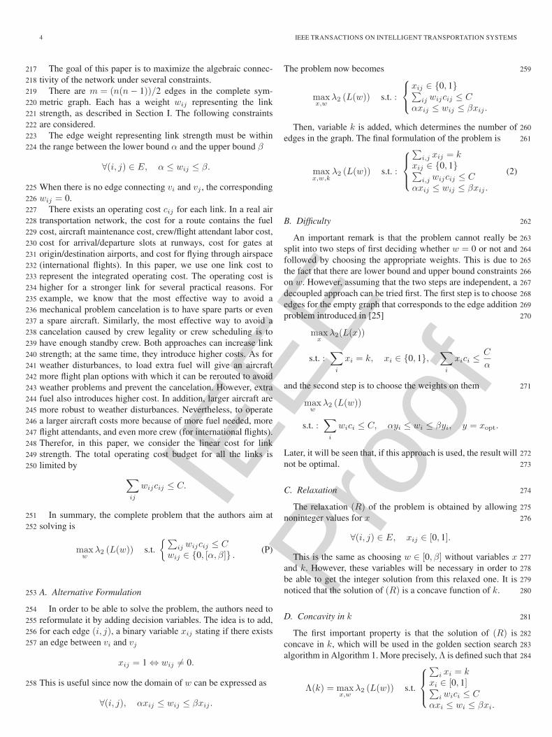
Fig. 9. Optimal result for a 30-node graph.

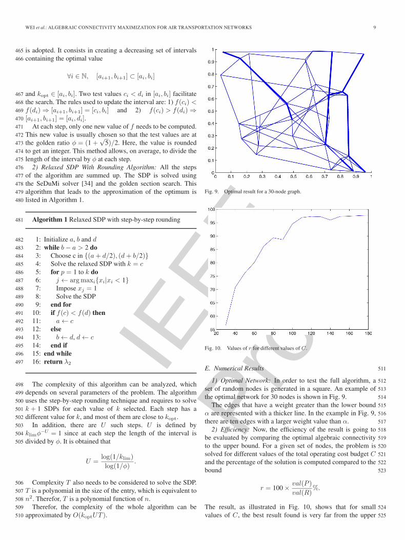
Fig. 10. Values of r for different values of C.

E. Numerical Results 511

1) Optimal Network: In order to test the full algorithm, a 512

set of random nodes is generated in a square. An example of 513

the optimal network for 30 nodes is shown in Fig. 9. 514

The edges that have a weight greater than the lower bound 515

α are represented with a thicker line. In the example in Fig. 9, 516

there are ten edges with a larger weight value than α. 517

2) Efficiency: Now, the efficiency of the result is going to 518

be evaluated by comparing the optimal algebraic connectivity 519

to the upper bound. For a given set of nodes, the problem is 520

solved for different values of the total operating cost budget C 521

and the percentage of the solution is computed compared to the 522

bound 523

r = 100 × val(P )

val(R)%.

The result, as illustrated in Fig. 10, shows that for small 524

values of C, the best result found is very far from the upper 525

IEEE

Proo

f

10 IEEE TRANSACTIONS ON INTELLIGENT TRANSPORTATION SYSTEMS

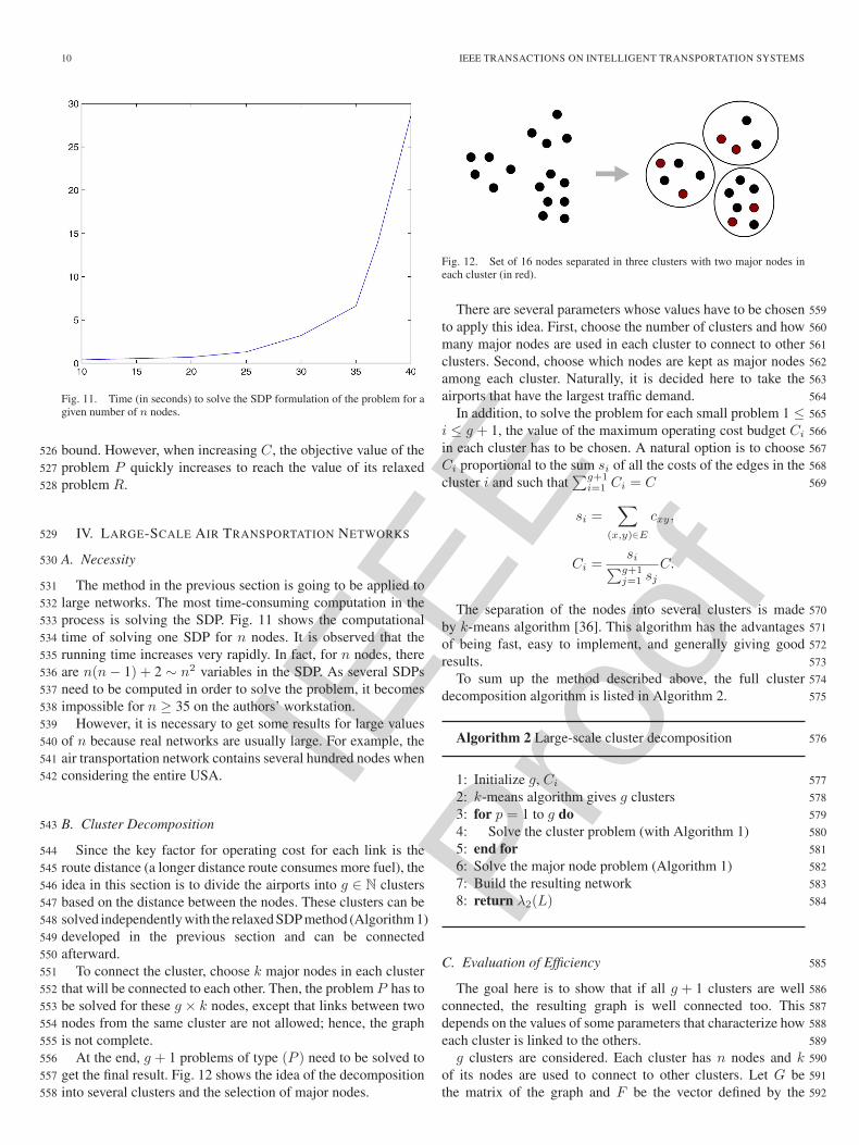
Fig. 11. Time (in seconds) to solve the SDP formulation of the problem for agiven number of n nodes.

bound. However, when increasing C, the objective value of the526

problem P quickly increases to reach the value of its relaxed527

problem R.528

IV. LARGE-SCALE AIR TRANSPORTATION NETWORKS529

A. Necessity530

The method in the previous section is going to be applied to531

large networks. The most time-consuming computation in the532

process is solving the SDP. Fig. 11 shows the computational533

time of solving one SDP for n nodes. It is observed that the534

running time increases very rapidly. In fact, for n nodes, there535

are n(n− 1) + 2 ∼ n2 variables in the SDP. As several SDPs536

need to be computed in order to solve the problem, it becomes537

impossible for n ≥ 35 on the authors’ workstation.538

However, it is necessary to get some results for large values539

of n because real networks are usually large. For example, the540

air transportation network contains several hundred nodes when541

considering the entire USA.542

B. Cluster Decomposition543

Since the key factor for operating cost for each link is the544

route distance (a longer distance route consumes more fuel), the545

idea in this section is to divide the airports into g ∈ N clusters546

based on the distance between the nodes. These clusters can be547

solved independently with the relaxed SDP method (Algorithm 1)548

developed in the previous section and can be connected549

afterward.550

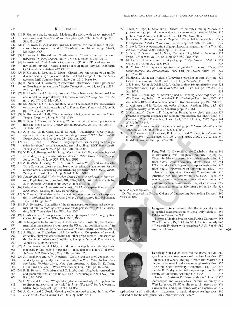
To connect the cluster, choose k major nodes in each cluster551

that will be connected to each other. Then, the problem P has to552

be solved for these g × k nodes, except that links between two553

nodes from the same cluster are not allowed; hence, the graph554

is not complete.555

At the end, g + 1 problems of type (P ) need to be solved to556

get the final result. Fig. 12 shows the idea of the decomposition557

into several clusters and the selection of major nodes.558

Fig. 12. Set of 16 nodes separated in three clusters with two major nodes ineach cluster (in red).

There are several parameters whose values have to be chosen 559

to apply this idea. First, choose the number of clusters and how 560

many major nodes are used in each cluster to connect to other 561

clusters. Second, choose which nodes are kept as major nodes 562

among each cluster. Naturally, it is decided here to take the 563

airports that have the largest traffic demand. 564

In addition, to solve the problem for each small problem 1 ≤ 565

i ≤ g + 1, the value of the maximum operating cost budget Ci 566

in each cluster has to be chosen. A natural option is to choose 567

Ci proportional to the sum si of all the costs of the edges in the 568

cluster i and such that∑g+1

i=1 Ci = C 569

si =∑

(x,y)∈Ecxy,

Ci =si∑g+1j=1 sj

C.

The separation of the nodes into several clusters is made 570

by k-means algorithm [36]. This algorithm has the advantages 571

of being fast, easy to implement, and generally giving good 572

results. 573

To sum up the method described above, the full cluster 574

decomposition algorithm is listed in Algorithm 2. 575

Algorithm 2 Large-scale cluster decomposition 576

1: Initialize g, Ci 577

2: k-means algorithm gives g clusters 578

3: for p = 1 to g do 579

4: Solve the cluster problem (with Algorithm 1) 580

5: end for 581

6: Solve the major node problem (Algorithm 1) 582

7: Build the resulting network 583

8: return λ2(L) 584

C. Evaluation of Efficiency 585

The goal here is to show that if all g + 1 clusters are well 586

connected, the resulting graph is well connected too. This 587

depends on the values of some parameters that characterize how 588

each cluster is linked to the others. 589

g clusters are considered. Each cluster has n nodes and k 590

of its nodes are used to connect to other clusters. Let G be 591

the matrix of the graph and F be the vector defined by the 592

IEEE

Proo

f

WEI et al.: ALGEBRAIC CONNECTIVITY MAXIMIZATION FOR AIR TRANSPORTATION NETWORKS 11

Fig. 13. (a) λ2 = f(n); (b) λ2 = f(k); (c) λ2 = f(g).

expression below. If, for instance, g = 3, matrix G can be put593

into the following form:594

G =

⎛⎜⎜⎜⎜⎜⎜⎜⎜⎜⎜⎝

E 0 0 E 0 0A1 0 0 0 0 0 0

0 0 0 0 0 0E 0 0 E 0 00 0 0 A2 0 0 00 0 0 0 0 0E 0 0 E 0 00 0 0 0 0 0 A3

0 0 0 0 0 0

⎞⎟⎟⎟⎟⎟⎟⎟⎟⎟⎟⎠

F =

⎛⎜⎜⎜⎜⎜⎜⎜⎜⎜⎜⎜⎝

αeβeβe000

−αe−βe−βe

⎞⎟⎟⎟⎟⎟⎟⎟⎟⎟⎟⎟⎠

with the following notation. e is the all-one vector. α and β are595

constants that will be computed in the next paragraph. A1, A2,596

and A3 represent the adjacency matrices of the three clusters.597

E is a k × k matrix with all elements equal to 1.598

1) Fiedler Vector: The Fiedler vector is the vector solution599

of the minimization problem600

minx∈Rn

{xTLx|‖x‖ = 1, xe = 0

}.

It is known to be an indicator on how to split a graph into two601

smaller graphs. In fact, the nodes that have the same sign in this602

vector form a cut of the graph (see [37]).603

Here, the optimal cut will naturally be found between two604

clusters. Since some of the nodes play the same role, the Fiedler605

vector has a shape close to F where α and β are constants that606

need to be determined.607

This assumption has been verified by numerical experiments608

and it seems to be a very good approximation of the real Fiedler609

vector.610

2) Computing the Connectivity: Consider that the Fiedler611

vector has the form of F and matrices are full, which means612

all nondiagonal elements are equal to 1. The matrix products 613

give 614

λ2 =FTLF,

λ2 = 2kαX + 2(n− k)βY

with 615

X =α (n− 1 + k(g − 1))− (k − 1)α− (n− k)β + kα,

Y =β(n− 1)− kα− (n− k − 1)β.

It is also known that ‖F‖ = 1; thus 616

2kα2 + (2n− 2k)β2 = 1,

α =

√1 − (2n− 2k)β

2k.

Substitute α with this expression and β is given by the 617

d λ2

d β= 0. (7)

With a computation software package like Maple, this gives 618

us the expression of function f such that 619

λ2 = f(n, k, g).

3) Resulted Curves: By solving (7), the values of α, β, and 620

λ2 are obtained. The following figures have been obtained with 621

Maple. Among the three parameters k, g, and n, fix two of them 622

and let the third one vary to see its influence on connectivity. 623

Fig. 13 provides a clearer idea on how to choose the value 624

of each parameter. For example, connectivity is almost linear 625

regarding k but has a concave shape when represented as a 626

function of the number of clusters g. 627

There exists a tradeoff: If g is too large, kg will be too large to 628

be solved. On the contrary, if g is too small, each of the cluster 629

will have too many nodes to be solved. 630

4) Numerical Results: The data used are the 100 largest 631

cities in the United States. Fig. 14 shows the 100 biggest 632

cities without any link. The cluster decomposition is used to 633

divide these 100 cities into g = 5 groups. In each group, we 634

selected k = 5. The lower bound α = 2 and the upper bound 635

IEEE

Proo

f

12 IEEE TRANSACTIONS ON INTELLIGENT TRANSPORTATION SYSTEMS

Fig. 14. Shown are the 100 largest cities in the USA.

Fig. 15. Result for the 100 largest cities in the USA.

β = 10. The total running time is 317 s with MATLAB on our636

workstation. The algebraic connectivity that we have achieved637

is λ2 = 2.6.638

The optimal network found is illustrated in Fig. 15. The blue639

lines represent the edges inside each cluster and the red lines640

represent the edges that connect nodes from different clusters.641

In a real network, most airlines use spoke-hub planning, in642

which the regional airports are clustered and connected to their643

regional hub airport. Fig. 15 shows the same behavior that644

regional airports are clustered together. In a real network in the645

United States, the number of the major nodes k for each cluster646

is usually 1, which means that the hub airport is the only major647

node for its cluster. In a real network in Europe, the number of648

the major nodes k is usually bigger than 1. In fact, the number649

k in a European network is those hub airports in each country.650

For example, Air France has hubs at Paris and Lyon (k = 2)651

and Air Berlin has its hubs at Berlin, Düsseldorf, Hamburg, and652

Munich (k = 4). In summary, the result in Fig. 15 is a practical653

design, and more importantly, the computation is very efficient654

for large-scale network planning.655

V. DIRECTED AIR TRANSPORTATION NETWORK 656

A. From Undirected Graph to Directed Graph 657

In this section, the methods are extended in directed graphs. 658

In order to be consistent with the undirected case, the graphs 659

need to be balanced, which means that the number of aircraft 660

that comes in is the same as the number of aircraft that leaves 661

the airport 662

∀i ∈ {1, . . . , n},n∑

j=1

wij =n∑

k=1

wki.

It is clear that the set of undirected graphs is included in the set 663

of directed balanced graphs. Therefor, the results should be at 664

least as good as in the previous section. 665

Definition: According to [38], if Ω = {x ∈ Rn, xe = 666

0, ‖x‖ = 1}, the definition of the algebraic connectivity can be 667

extended for directed balanced graphs with 668

minx∈Ω

xTLx = λ2

(12(L+ LT )

).

Property 4: In the directed case and with this definition 669

of the algebraic connectivity, the upper bound given by the 670

continuous relaxation is the same as in the undirected case. 671

Proof: Given the optimum directed balanced graph in the 672

relaxed problem and its incidence matrix G, H can be created 673

H =G+GT

2

where H is symmetric and satisfies all the constraints of the 674

problem since they are linear. In addition with the definition of 675

the connectivity for directed graphs, the connectivity of H is 676

clearly the same as the connectivity of G. 677

Since it is also known that undirected graphs are a subset of 678

directed balanced graphs, the bounds are equal in both cases. 679

This will allow us to easily evaluate the improvement brought 680

by directed graphs. � 681

B. Results 682

The same method is used as in Section III. The results are 683

impressively better with directed graphs, as shown in Fig. 16. 684

The best value for the directed balanced case almost reached 685

the upper bound. It is also noticed that the optimal result has 686

less edges than the optimal network in the undirected case (an 687

edge in the undirected case is counted in both ways). 688

It is shown in Fig. 17 that most of the edges in the optimal 689

solution are oriented in only one way, which shows that the 690

solution is very different from the undirected case. 691

However, there is an important drawback. Indeed, two times 692

as many variables are needed for directed networks. Thus, the 693

problem takes a much longer time to be solved and is only 694

applicable on smaller networks. 695

IEEE

Proo

f

WEI et al.: ALGEBRAIC CONNECTIVITY MAXIMIZATION FOR AIR TRANSPORTATION NETWORKS 13

Fig. 16. λ = f(k) for the same graph with different approaches.

Fig. 17. Optimal directed graph.

C. Failure Case696

If an edge or a node is removed, the graph is not balanced697

anymore. This can cause important problems in practice; hence,698

the remaining weights in the graph need to be changed to handle699

this problem.700

This operation can be done by using a flow algorithm. The701

first step is to link the nodes with positive aircraft balance to a702

virtual source and those with negative balance to a sink. The ca-703

pacities of these links are equal to the absolute value of the704

difference in the balance flow for the node. The capacity of the705

other links of the graph is β.706

Then, consider the problem of the maximization of the flow707

from the source to the sink. This problem can be solved by using708

Edmonds–Karp algorithm [39], which has efficient complexity,709

i.e., O(nm2). This algorithm maintains the balance of the flow710

at each node.711

At the end, the graph is the graph solution of the flow712

problem when the source and the sink are removed. Figs. 18713

and 19 show an example of a graph in which a node is removed,714

Fig. 18. Example of a graph with a node failure.

Fig. 19. Example of a graph after maximization of the flow.

before and after maximization of the flow. The graph in Fig. 19 715

is now balanced by Edmonds–Karp algorithm after removing 716

the source (green node) and the sink (blue node). 717

VI. CONCLUSION 718

In this paper, a new problem concerning the maximization of 719

the algebraic connectivity of a network has been presented and 720

studied. This problem consists of finding both the edges of the 721

graph and their weight assignment under several constraints. 722

First, the problem in small networks is exactly solved, and it is 723

shown that the problem cannot be separated into two already 724

studied independent problems. Then, a relaxed SDP method 725

with step-by-step rounding is presented to solve the problem 726

approximately for better computational efficiency. With the 727

method developed for small-scale network, the cluster decom- 728

position method is proposed to solve the large-scale network 729

problem and successfully find the near-optimal solution for a 730

network of the 100 largest cities in the United States. Finally, 731

the study is extended to directed graphs. Numerical experiments 732

and analysis are performed for all the proposed algorithms. The 733

developed methods are able to model and maximize robustness 734

in air transportation networks for airlines and for the NAS. They 735

also provide an option to improve current ways of the generic 736

network design. 737

IEEE

Proo

f

14 IEEE TRANSACTIONS ON INTELLIGENT TRANSPORTATION SYSTEMS

REFERENCES738

[1] R. Guimera and L. Amaral, “Modeling the world-wide airport network,”739Eur. Phys. J. B, Condens. Matter Complex Syst., vol. 38, no. 2, pp. 381–740385, Mar. 2004.741

[2] R. Kincaid, N. Alexandrov, and M. Holroyd, “An investigation of syn-742chrony in transport networks,” Complexity, vol. 14, no. 4, pp. 34–43,743Mar./Apr. 2008.744

[3] E. Vargo, R. Kincaid, and N. Alexandrov, “Towards optimal transport745networks,” J. Syst., Cybern. Inf., vol. 8, no. 4, pp. 59–64, Jul. 2010.746

[4] International Civil Aviation Organization (ICAO), “Procedures for air747navigation services—Rules of the air and air traffic services,” Montréal,748QC, Canada, doc 4444-RAC/501, 2010.749

[5] P. Kostiuk, D. Lee, and D. Long, “Closed loop forecasting of air traffic750demand and delay,” presented at the 3rd USA/Europe Air Traffic Man-751agement R&D Seminar, Napoli, Italy, Jun. 2010, Paper 80.752

[6] K. Nam and T. Schaefer, “Forecasting international airline passenger753traffic using neural networks,” Logist. Transp. Rev., vol. 31, no. 3, pp. 239–754251, Sep. 1995.755

[7] F. Alamdari and S. Fagan, “Impact of the adherence to the original low756cost model on the profitability of low cost airlines,” Transp. Rev., vol. 25,757no. 3, pp. 377–392, May 2005.758

[8] M. Dresner, J.-S. C. Lin, and R. Windle, “The impact of low-cost carriers759on airport and route competition,” J. Transp. Econ. Policy, vol. 30, no. 3,760pp. 309–328, Sep. 1996.761

[9] K. Button and S. Lall, “The economics of being an airport hub city,” Res.762Transp. Econ., vol. 5, pp. 75–105, 1999.763

[10] T. Oum, A. Zhang, and Y. Zhang, “A note on optimal airport pricing in a764hub-and-spoke system,” Transp. Res. B, Methodol., vol. 30, no. 1, pp. 11–76518, Feb. 1996.766

[11] X.-B. Hu, W.-H. Chen, and E. Di Paolo, “Multiairport capacity man-767agement: Genetic algorithm with receding horizon,” IEEE Trans. Intell.768Transp. Syst., vol. 8, no. 2, pp. 254–263, Jun. 2007.769

[12] X.-B. Hu and E. Di Paolo, “Binary-representation-based genetic algo-770rithm for aircraft arrival sequencing and scheduling,” IEEE Trans. Intell.771Transp. Syst., vol. 9, no. 2, pp. 301–310, Jun. 2008.772

[13] Y. Eun, I. Hwang, and H. Bang, “Optimal arrival flight sequencing and773scheduling using discrete airborne delays,” IEEE Trans. Intell. Transp.774Syst., vol. 11, no. 2, pp. 359–373, Jun. 2010.775

[14] Z.-H. Zhan, J. Zhang, Y. Li, O. Liu, S. Kwok, W. Ip, and O. Kaynak,776“An efficient ant colony system based on receding horizon control for the777aircraft arrival sequencing and scheduling problem,” IEEE Trans. Intell.778Transp. Syst., vol. 11, no. 2, pp. 399–412, Jun. 2010.779

[15] FlightStats-Global Flight Tracker, Status Tracking and Airport Informa-780tion, FlightStats, Inc., Portland, OR, USA, 2013, retrieved on March 16,7812013. [Online]. Available: http://www.flightstats.com782

[16] Federal Aviation Administration (FAA), “FAA Aerospace Forecasts FY7832008-2025,” Washington, DC, USA, Dec. 2010.784

[17] S. Conway, “Scale-free networks and commercial air carrier transporta-785tion in the United States,” in Proc. 24th Int. Congr. Aeron. Sci., Yokohama,786Japan, 2004, pp. 1–12.787

[18] P. A. Bonnefoy, “Scalability of the air transportation system and develop-788ment of multi-airport systems: A worldwide perspective,” Ph.D. disserta-789tion, MIT, Cambridge, MA, USA, Jun. 2008.790

[19] N. Alexandrov, “Transportation network topologies,” NASA Langley Res.791Center, Hampton, VA, USA, Tech. Rep., 2004.792

[20] T. Kotegawa, D. DeLaurentis, K. Noonan, and J. Post, “Impact of com-793mercial airline network evolution on the US air transportation system,” in794Proc. 9th USA/Europe ATM Res. Develop. Semin., Berlin, Germany, 2011.AQ3 795

[21] A. Bigdeli, A. Tizghadam, and A. Leon-Garcia, “Comparison of network796criticality, algebraic connectivity, and other graph metrics,” presented at797the 1st Annu. Workshop Simplifying Complex Network Practitioners,798Venice, Italy, 2009, Paper 4.799

[22] A. Jamakovic and S. Uhlig, “On the relationship between the algebraic800connectivity and graph’s robustness to node and link failures,” in Proc.8013rd EuroNGI Netw. Conf., May 2007, pp. 96–102.802

[23] A. Jamakovic and P. V. Mieghem, “On the robustness of complex net-803works by using the algebraic connectivity,” in Proc. Netw. Ad Hoc Sen-804sor Netw., Wireless Netw., Next Gen. Internet, A. Das, H. K. Pung,805F. Bu Sung Lee, and L. Wong Wai Choong, Eds., 2008, pp. 183–194.806

[24] R. H. Byrne, J. T. Feddema, and C. T. Abdallah, “Algebraic connectivity807and graph robustness,” Sandia Nat. Lab., Albuquerque, NM, USA, Tech.808Rep., Jul. 2009.809

[25] P. Wei and D. Sun, “Weighted algebraic connectivity: An application810to airport transportation network,” in Proc. 18th IFAC World Congress,811Milan, Italy, Aug. 2011, pp. 13 864–13 869.812

[26] A. Ghosh and S. Boyd, “Growing well-connected graphs,” in Proc. 45th813IEEE Conf. Decis. Control, Dec. 2006, pp. 6605–6611.814

[27] J. Sun, S. Boyd, L. Xiao, and P. Diaconis, “The fastest mixing Markov 815process on a graph and a connection to a maximum variance unfolding 816problem,” SIAM Rev., vol. 48, no. 4, pp. 681–699, Nov. 2006. 817

[28] F. Goring, C. Helmberg, and M. Wappler, “Embedded in the shadow of 818the separator,” SIAM J. Optim., vol. 19, no. 1, pp. 472–501, Feb. 2008. 819

[29] S. Boyd, “Convex optimization of graph Laplacian eigenvalues,” in Proc. 820Int. Congr. Math., 2006, vol. 3, pp. 1311–1319. 821

[30] S. Boyd, P. Diaconis, and L. Xiao, “Fastest mixing Markov chain on a 822graph,” SIAM Rev., vol. 46, no. 4, pp. 667–689, Dec. 2004. 823

[31] M. Fiedler, “Algebraic connectivity of graphs,” Czechoslovak Math. J., 824vol. 23, no. 98, pp. 298–305, 1973. 825

[32] B. Mohar, “The Laplacian spectrum of graphs,” in Graph Theory, 826Combinatorics, and Applications. New York, NY, USA: Wiley, 1991, 827pp. 871–898. 828

[33] M. Siotani, “Some applications of Loewner’s ordering on symmetric ma- 829trices,” Ann. Inst. Stat. Math., vol. 19, no. 1, pp. 245–259, Dec. 1967. 830

[34] J. F. Sturm, “Using SeDuMi 1.02, A Matlab toolbox for optimization over 831symmetric cones,” Optim. Methods Softw., vol. 11, no. 1–4, pp. 625–653, 832Jan. 1999. 833

[35] W. Press, S. Teukolsky, W. Vetterling, and B. Flannery, The Art of Scien- 834tific Computing, 3rd ed. Cambridge, U.K.: Cambridge Univ. Press, 2007. 835ch. Section 10.2. Golden Section Search in One Dimension, pp. 492–496. 836

[36] J. Kleinberg and E. Tardos, Algorithm Design. Reading, MA, USA: 837Addison-Wesley, 2005, ch. 4.7 Clustering, pp. 157–161. 838

[37] S. Martinez, G. Chatterji, D. Sun, and A. Bayen, “A weighted graph ap- 839proach for dynamic airspace configuration,” presented at the AIAA Conf. 840Guidance, Control Dynamics, Hilton Head, SC, USA, Aug. 2007, Paper 841AIAA 2007-6448. 842

[38] C. Wu, “Algebraic connectivity of directed graphs,” Linear Multilinear 843Algebra, vol. 53, no. 3, pp. 203–223, Jun. 2005. 844

[39] T. H. Cormen, C. E. Leiserson, R. L. Rivest, and C. Stein, Introduction 845to Algorithms. Cambridge, MA, USA: MIT Press, 2009, ch. 26.2 The 846Ford-Fulkerson method, pp. 727–730. 847

Peng Wei (M’12) received the Bachelor’s degree 848in automation from Tsinghua University, Beijing, 849China; the Master’s degree in electrical engineering 850from Stony Brook University, Stony Brook, NY, 851USA; and the Ph.D. degree in aerospace engineering 852from Purdue University, West Lafayette, IN, USA. 853

He is an Operations Research Consultant with 854American Airlines, Fort Worth, TX, USA. His re- 855search interests include next-generation air trans- 856portation system, environmental impact of aviation, 857and unmanned aerial vehicle integration in the Na- 858

tional Airspace System. 859Dr. Wei received the Purdue College of Engineering Outstanding Research 860

Award in 2013. 861

Gregoire Spiers received the Bachelor’s degree 862in applied mathematics from École Polytechnique, 863Palaiseau, France, in 2012. 864

He was a Visiting Student with Purdue University, 865West Lafayette, IN, USA, in 2011. He is currently 866a Research Engineer with Amadeus S.A.S., Sophia 867Antipolis, France. AQ4868

Dengfeng Sun (M’08) received the Bachelor’s de- 869gree in precision instruments and mechanology from 870Tsinghua University, Beijing, China; the Master’s 871degree in industrial and systems engineering from 872The Ohio State University, Columbus, OH, USA; 873and the Ph.D. degree in civil engineering from Uni- 874versity of California, Berkeley, CA, USA. 875

He is an Assistant Professor with the School of 876Aeronautics and Astronautics, Purdue University, 877West Lafayette, IN, USA. His research interests in- 878clude control and optimization, with an emphasis on 879

applications in air traffic flow management, dynamic airspace configuration, 880and studies for the next-generation air transportation system. 881

IEEE

Proo

f

AUTHOR QUERIES

AUTHOR PLEASE ANSWER ALL QUERIES

AQ1 = Please provide keywords.AQ2 = Please check if changes made in the affiliation note of author Gregoire Spiers are appropriate, with

reference to the given biography. Please also check accuracy of postal code and location.AQ3 = Please provide page range in Ref. [20].AQ4 = Please check accuracy of provided location.

END OF ALL QUERIES

IEEE

Proo

f

IEEE TRANSACTIONS ON INTELLIGENT TRANSPORTATION SYSTEMS 1

Algebraic Connectivity Maximization for AirTransportation Networks

1

2

Peng Wei, Member, IEEE, Gregoire Spiers, and Dengfeng Sun, Member, IEEE3

Abstract—It is necessary to design a robust air transportation4network. An experiment based on the real air transportation5network is performed to show that algebraic connectivity is a fair6measure for network robustness under random failures. Therefor,7the goal of this paper is to maximize algebraic connectivity. Some8researchers solve the maximization of the algebraic connectivity9by choosing the weights for the edges in the graph. Others focus10on the best way to add edges in a network in order to optimize11the connectivity. In this paper, the authors formulate a new air12transportation network model and show that the corresponding13algebraic connectivity optimization problem is interesting because14the two subproblems of adding edges and choosing edge weights15cannot be treated separately. The new problem is formulated and16exactly solved in a small air transportation network case. The17authors also propose the approximation algorithm in order to18achieve better efficiency. For large networks, the semidefinite pro-19gramming with cluster decomposition is first presented. Moreover,20the algebraic connectivity maximization for directed networks21is discussed. Simulations are performed for a small-scale case,22large-scale problem, and directed network problem.23

Index Terms—Author, please supply index terms/keywords24for your paper. To download the IEEE Taxonomy go to http:25//www.ieee.org/documents/Taxonomy_v101.pdf.AQ1 26

I. INTRODUCTION27

AN AIR transportation network consists of distinct airports28

(cities) and direct flight routes between airport pairs [1].29

Usually, a graph G(V,E) is used to describe an air trans-30

portation network [2], [3], where the node set V represents all31

the n airports and the edge (link) set E represents all the m32

direct flight routes between airports. If a direct flight route from33

airport a to airport b exists, normally, the direct return route34

from airport b to airport a also exists [4]; G(V,E) is constructed35

as an undirected simple graph, where the airports are indexed36

as {vi|i = 1, 2, . . . , n} and the direct flight routes are named37

as eij if there is a direct route between airports vi and vj .38

There are many factors to be considered when designing an air39

transportation network, such as traffic demand, operating cost,40

airport hubs, market competition, multiairport systems, and41

Manuscript received November 6, 2012; revised April 5, 2013 andAugust 20, 2013; accepted October 1, 2013. The Associate Editor for this paperwas J.-P. B. Clarke.

P. Wei is with the Operations Research and Advanced Analytics, AmericanAirlines, Fort Worth, TX 76155 USA (e-mail: peng.wei@aa.com).

G. Spiers was with the Department of Applied Mathematics, École Polytech-nique, 91120 Palaiseau, France. He is now with Amadeus S.A.S., 06902 SophiaAntipolis, France (e-mail: gregoire.spiers@polytechnique.org).AQ2

D. Sun is with the School of Aeronautics and Astronautics, Purdue Univer-sity, West Lafayette, IN 47907 USA (e-mail: dsun@purdue.edu).

Color versions of one or more of the figures in this paper are available onlineat http://ieeexplore.ieee.org.

Digital Object Identifier 10.1109/TITS.2013.2284913

Fig. 1. Air transportation network route map for Virgin America Airlines.

scheduling [5]–[14]. In this paper, we focus on investigating 42

the network robustness maximization, particularly the algebraic 43

connectivity maximization. 44

A. Algebraic Connectivity and Air Transportation 45

Network Robustness 46

In order to illustrate the relationship between the algebraic 47

connectivity and air transportation network robustness, a real 48

air transportation network of Virgin America is studied. The 49

following experiment shows that algebraic connectivity is a 50

fair measurement for the network robustness with regard to 51

random link failures under the current Virgin America network 52

topology. 53

According to the current route map of Virgin America in 54

Fig. 1, we consider the 16 airports in the United States and 55

obtain the adjacency matrix as Table I. The 16 United States air- 56

ports include Boston (BOS), New York City/John F. Kennedy 57

(JFK), Philadelphia, Washington Dulles International Air- 58

port (DC/IAD), Ronald Reagan Washington National Airport 59

(DC/DCA), Chicago O’Hare International Airport (ORD), 60

Orlando, Fort Lauderdale, Dallas/Fort Worth, Seattle, Portland, 61

San Francisco, Los Angeles, Las Vegas, San Diego, and Palm 62

Springs and are indexed as numbers 1–16. San Francisco Inter- 63

national Airport (SFO) and Los Angeles International Airport 64

(LAX) are two major hubs of the entire network. Both have at 65

least one direct flight to almost all the other airports. 66

In order to show how well the algebraic connectivity can 67

measure the robustness of an air transportation network, we 68

1524-9050 © 2013 IEEE

IEEE

Proo

f

2 IEEE TRANSACTIONS ON INTELLIGENT TRANSPORTATION SYSTEMS

TABLE IADJACENCY MATRIX CONSISTS OF 16 VIRGIN AMERICA AIRLINES AIRPORTS IN THE USA

created six different weighted air transportation networks with69

the same topology in Table I by randomly assigning one of70

the three types of link weights to each route. Each link weight71

is an indication of link strength. A larger weight represents a72

stronger link and a smaller weight shows that the corresponding73

link is easier to fail. There are many reasons for route failure,74

such as weather disturbance, long ground delay program, long75

airspace flow program (AFP), aircraft mechanical problem, and76

upline flight delay/cancelation. The route failure rate statis-77

tics are published by each origin–destination pair (route) and78

different routes have different features [15]. For example, the79

route failure rate between JFK and BOS during summer is80

higher than that between SFO and LAX because of the crowded81

northeastern airspace (AFP is more frequent) and more summer82

thunderstorms. Another example is that a shorter route is easier83

to fail than a longer transcontinental route because: 1) airlines84

usually put larger aircraft on transcontinental route, and these85

aircraft are more robust to weather disturbance and 2) airlines86

are more likely to cancel shorter route flights because the flight87

frequency on a shorter route is higher; therefor, the passengers88

on the canceled flight are easier to protect (be reaccommodated89

to later flights). In summary, each route has its own features90

and thus in our model we consider that they have different91

possibilities for failure.92

The three types of link weights are mapped to different link93

failure probabilities (see Table II). The link failure probability94

range [%0, %5] is obtained from the historical flight cancelation95

rate between September 15, 2012, and November 15, 2012 [15].96

A network failure is defined as the existence of at least one97

pair of nodes that cannot access each other through any one or98

multiple links. For each one of the six weighted networks, 100099

trials are performed. In each trial, every link fails randomly100

TABLE IIMAPPING BETWEEN LINK WEIGHTS AND LINK FAILURE PROBABILITIES

TABLE IIINETWORK FAILURE NUMBERS WITH DIFFERENT ALGEBRAIC

CONNECTIVITY VALUES

according to the failure probabilities listed in Table II. The total 101

number of network failures is counted in 1000 random trials. 102

The results are shown in Table III with algebraic connectivity 103

sorted in ascending order. 104

We can see that with higher algebraic connectivity, the 105

network is more robust and has fewer network failures. With 106

lower weighted algebraic connectivity, the network is easier to 107

break down. Therefor, algebraic connectivity is a fair robustness 108

measure for the air transportation network, and we need to find 109

the maximized algebraic connectivity. 110

The air traffic demand is expected to continue its rapid 111

growth in the future. The Federal Aviation Administration 112

estimated that the number of passengers is projected to increase 113

by an average of 3% every year until 2025 [16]. The expanding 114

traffic demand on the current air transportation networks of 115

different airlines will cause more and more flight cancelations 116

with the limited airport and airspace capacities. As a result, 117

more robust air transportation networks are desired to sustain 118

IEEE

Proo

f

WEI et al.: ALGEBRAIC CONNECTIVITY MAXIMIZATION FOR AIR TRANSPORTATION NETWORKS 3

the increasing traffic demand for each airline and for the entire119

National Airspace System (NAS). This is the major motivation120

of this paper.121

B. Related Work122

An air transportation network and its robustness have been123

studied over the last several years. Guimera and Amaral first124

studied the scale-free graphical model of the air transportation125

network [1]. Conway showed that it was better to describe126

the national air transportation system or the commercial air127

carrier transportation network as a system of systems [17].128

Bonnefoy showed that the air transportation network was scale129

free with aggregating multiple airport nodes into meganodes130

[18]. Alexandrov defined that on-demand transportation net-131

works would require robustness in system performance [19].132

The robustness of an on-demand network would depend on the133

tolerance of the network to variability in temporal and spatial134

dynamics of weather, equipment, facility, crew positioning, etc.135

Kotegawa et al. surveyed different metrics for air transportation136

network robustness, including betweenness, degree, centrality,137

connectivity, etc. [20]. They selected clustering coefficient and138

eigenvector centrality as the network robustness metrics in139

their machine learning approach. Bigdeli et al. compared alge-140

braic connectivity, network criticality, average degree, average141

node betweenness, and other metrics [21]. Jamakovic et al.142

found that algebraic connectivity was an important metric in143

the analysis of various robustness problems in several typical144

network models [22], [23]. Byrne et al. showed that algebraic145

connectivity was the efficient measure for the robustness of146

both small and large networks [24]. Vargo et al. in [3] chose147

algebraic connectivity as the robustness metric and built the148

optimization problem solved by the edge swapping-based tabu149

search algorithm.150

In this paper, we measure the robustness of air transportation151

network by computing the algebraic connectivity, which is152

usually considered as one of the most reasonable and efficient153

evaluation methods [24], [25]. Although the maximized value154

of algebraic connectivity is abstract, the optimized air trans-155

portation network structure and weighting assignment provide156

us the applicable design.157

There are some literature on algebraic connectivity maxi-158

mization. The problems studied can be divided into two cat-159

egories, namely, the edge addition problem and the variable160

weights problem.161

1) Edge addition problem: The goal is to add or remove a162

given number of k edges on a graph in order to get the best163

algebraic connectivity. The edges to be added or removed164

are selected from a candidate set. The algorithms that165

have been developed to solve the problem include tabu166

search [25], greedy algorithms [25], [26], and rounded167

semidefinite programming (SDP) [26].168

2) Variable weights problem: The edges of the graph are169

fixed and the goal is to determine the edge weights in170

order to maximize the algebraic connectivity. This is171

a convex optimization problem that is often solved by172

using an SDP formulation [27]–[29] or a subgradient173

algorithm [30].174

C. Contribution 175

The major contribution of this paper compared with what 176

has been studied is that we find that, in order to maximize 177

the algebraic connectivity, the edge addition problem and the 178

variable weights problem cannot be studied separately. Solving 179

one of them independently will only result in a suboptimal 180

solution. Therefor, we propose a new algorithm to solve both 181

problems at the same time. How to choose the edges of the 182

graph is demonstrated, as well as how to assign their weights. 183

In addition, we are the first to present the cluster decomposition 184

method to achieve better computation efficiency for large-scale 185

networks. We are also the first to discuss the algebraic connec- 186

tivity maximization for directed air transportation networks. 187

The rest of this paper is structured as follows. Section II 188

shows why this problem naturally arises in air transportation 189

networks and how it can be formulated. In Section III, the 190

problem is exactly solved for small networks, and the fact that 191

the two problems are not independent is highlighted. Then, the 192

authors present the SDP formulation and the more efficient full 193

algorithm, which includes relaxed SDP, and solution rounding 194

is proposed. In Section IV, the problem for large networks 195

is solved, the computational efficiency is analyzed, and the 196

numerical results are provided. The algebraic connectivity op- 197

timization for directed air transportation networks is presented 198

in Section V. Section VI concludes this paper. 199

II. PROBLEM FORMULATION 200

A graph G with n nodes and m edges is used to define an air 201

transportation network. Let A = (aij) be the adjacency matrix 202

of G. The Laplacian matrix L = (lij) of G is defined by 203{lij = −aij , if i �= jlii =

∑nj=1 aij .

The eigenvalues of L are sorted λ1 ≤ λ2 ≤ . . . ≤ λn. L is a 204

semidefinite positive matrix; thus, for all i, λi ≥ 0. It is also 205

known that λ1 = 0 since Le = 0 with e = (1, . . . , 1) [31]. 206

Definition: The second smallest eigenvalue λ2(L) is the 207

algebraic connectivity of G. 208

Now, recall the two key properties of the algebraic connec- 209

tivity that will be used in this paper. 210

Property 1: Let e = (1, . . . , 1) ∈ Rn and 211

Ω ={x ∈ R

n|‖x‖ = 1, eTx = 0}.

The Courant–Fischer principle [32] states that 212

λ2 = minx∈Ω

xTLx. (1)

Property 2: Function w → λ2(w) is concave with w denot- 213

ing the edge weight vector. This can be proven by seeing that 214

λ2(w) is the pointwise infimum of a family of linear functions 215

of w (see [27]) 216

λ2(w) = inf‖v‖=1,eT v=0

vTLv,

λ2(w) = inf‖v‖=1,eT v=0

∑(i,j)∈E

wij(vi − vj)2.

IEEE

Proo

f

4 IEEE TRANSACTIONS ON INTELLIGENT TRANSPORTATION SYSTEMS

The goal of this paper is to maximize the algebraic connec-217

tivity of the network under several constraints.218

There are m = (n(n− 1))/2 edges in the complete sym-219

metric graph. Each has a weight wij representing the link220

strength, as described in Section I. The following constraints221

are considered.222

The edge weight representing link strength must be within223

the range between the lower bound α and the upper bound β224

∀(i, j) ∈ E, α ≤ wij ≤ β.

When there is no edge connecting vi and vj , the corresponding225

wij = 0.226

There exists an operating cost cij for each link. In a real air227

transportation network, the cost for a route contains the fuel228

cost, aircraft maintenance cost, crew/flight attendant labor cost,229

cost for arrival/departure slots at runways, cost for gates at230

origin/destination airports, and cost for flying through airspace231

(international flights). In this paper, we use one link cost to232

represent the integrated operating cost. The operating cost is233

higher for a stronger link for several practical reasons. For234

example, we know that the most effective way to avoid a235

mechanical problem cancelation is to have spare parts or even236

a spare aircraft. Similarly, the most effective way to avoid a237

cancelation caused by crew legality or crew scheduling is to238

have enough standby crew. Both approaches can increase link239

strength; at the same time, they introduce higher costs. As for240

weather disturbances, to load extra fuel will give an aircraft241

more flight plan options with which it can be rerouted to avoid242

weather problems and prevent the cancelation. However, extra243

fuel also introduces higher cost. In addition, larger aircraft are244

more robust to weather disturbances. Nevertheless, to operate245

a larger aircraft costs more because of more fuel needed, more246

flight attendants, and even more crew (for international flights).247

Therefor, in this paper, we consider the linear cost for link248

strength. The total operating cost budget for all the links is249

limited by250 ∑ij

wijcij ≤ C.

In summary, the complete problem that the authors aim at251

solving is252

maxw

λ2 (L(w)) s.t.

{∑ij wijcij ≤ C

wij ∈ {0, [α, β]} . (P)

A. Alternative Formulation253

In order to be able to solve the problem, the authors need to254

reformulate it by adding decision variables. The idea is to add,255

for each edge (i, j), a binary variable xij stating if there exists256

an edge between vi and vj257

xij = 1 ⇔ wij �= 0.

This is useful since now the domain of w can be expressed as258

∀(i, j), αxij ≤ wij ≤ βxij .

The problem now becomes 259

maxx,w

λ2 (L(w)) s.t. :

⎧⎨⎩

xij ∈ {0, 1}∑ij wijcij ≤ C

αxij ≤ wij ≤ βxij .

Then, variable k is added, which determines the number of 260

edges in the graph. The final formulation of the problem is 261

maxx,w,k

λ2 (L(w)) s.t. :

⎧⎪⎨⎪⎩

∑i,j xij = k

xij ∈ {0, 1}∑i,j wijcij ≤ C

αxij ≤ wij ≤ βxij .

(2)

B. Difficulty 262

An important remark is that the problem cannot really be 263

split into two steps of first deciding whether w = 0 or not and 264

followed by choosing the appropriate weights. This is due to 265

the fact that there are lower bound and upper bound constraints 266

on w. However, assuming that the two steps are independent, a 267

decoupled approach can be tried first. The first step is to choose 268

edges for the empty graph that corresponds to the edge addition 269

problem introduced in [25] 270

maxx

λ2(L(x))

s.t. :∑i

xi = k, xi ∈ {0, 1},∑i

xici ≤C

α

and the second step is to choose the weights on them 271

maxw

λ2 (L(w))

s.t. :∑i

wici ≤ C, αyi ≤ wi ≤ βyi, y = xopt.

Later, it will be seen that, if this approach is used, the result will 272

not be optimal. 273

C. Relaxation 274

The relaxation (R) of the problem is obtained by allowing 275

noninteger values for x 276

∀(i, j) ∈ E, xij ∈ [0, 1].

This is the same as choosing w ∈ [0, β] without variables x 277

and k. However, these variables will be necessary in order to 278

be able to get the integer solution from this relaxed one. It is 279

noticed that the solution of (R) is a concave function of k. 280

D. Concavity in k 281

The first important property is that the solution of (R) is 282

concave in k, which will be used in the golden section search 283

algorithm in Algorithm 1. More precisely, Λ is defined such that 284

Λ(k) = maxx,w

λ2 (L(w)) s.t.

⎧⎪⎨⎪⎩

∑i xi = k

xi ∈ [0, 1]∑i wici ≤ C

αxi ≤ wi ≤ βxi.

IEEE

Proo

f

WEI et al.: ALGEBRAIC CONNECTIVITY MAXIMIZATION FOR AIR TRANSPORTATION NETWORKS 5

Property 3: Λ(k) is a concave function.285

This property is important since it shows that the maximiza-286

tion of the algebraic connectivity is related to the number of287

edges in the graph. By solving the problem for very few values288

of k, a good knowledge on kopt can be obtained.289

Proof: Consider k1 and k2 in R and γ ∈ [0, 1] such that290

Λ(ki) > 0 for i = 1, 2. The idea is to use the fact that w →291

λ2(L(w)) is concave (please see Property 2).292

Λ (γk1+(1−γ)k2)

=maxx,w

λ2 s.t.

⎧⎪⎨⎪⎩

∑i xi=γk1+(1−γ)k2

xi ∈ [0, 1]∑i wici≤C

αxi≤wi≤βxi

≥maxx,w

λ2 s.t.

⎧⎪⎪⎪⎪⎨⎪⎪⎪⎪⎩

∑i x

(1)i =k1,

∑i x

(2)i =k2

x(j)i ∈ [0, 1], j=1, 2

x=γx(1)+(1−γ)x(2)∑i wici≤C

αxi≤wi≤βxi

≥maxx,w

λ2 s.t.

⎧⎪⎪⎪⎪⎪⎨⎪⎪⎪⎪⎪⎩

∑i x

(1)i =k1,

∑i x

(2)i =k2

x(j)i ∈ [0, 1], j=1, 2

w=γw(1)+(1−γ)w(2)∑i wici≤C

αx(j)i ≤w

(j)i ≤βx

(j)i

≥γmaxx,w

λ2 s.t.

⎧⎪⎨⎪⎩

∑i xi=k1

xi ∈ [0, 1]∑i wici≤C

αxi≤wi≤βxi

+(1−γ)maxx,w

λ2 s.t.

⎧⎪⎨⎪⎩

∑i xi=k2

xi ∈ [0, 1]∑i wici≤C

αxi≤wi≤βxi

≥γΛ(k1)+(1−γ)Λ(k2)

which proves that Λ is concave in k. �293

III. SMALL-SCALE AIR TRANSPORTATION NETWORKS294

A. Exact Solution for Small Networks295

If all weights have to be chosen within an interval, the296

problem becomes a convex optimization problem and it can297

be solved using an SDP solver. The idea here is to try all the298

possible configurations for which all the weights are either 0299

or in [α, β]. Then, each configuration can be independently300

optimized and the one that leads to the best result can be found.301

Consider that n nodes are chosen randomly. There are m =302

(n(n− 1))/2 edges and 2m configurations to test. For each303

configuration, if Y is the set of the edges that are actually in304

the graph, the following problem needs to be solved:305

maxw

λ2 (L(w)) s.t.

⎧⎨⎩

∑ij wijcij ≤ C

α ≤ wij ≤ β, ∀(i, j) ∈ Ywij = 0, ∀(i, j) /∈ Y .

Fig. 2. Results of (k, λ2) for all the configurations of n = 5 and C = 6.5.

Fig. 3. Results of (k, λ2) for all the configurations of n = 6 and C = 8.

This can be done by solving the SDP corresponding to the 306

weight optimization problem (see [27] for details) 307

minw

∑i

wici s.t.

⎧⎨⎩

α ≤ wi ≤ β, ∀(i, j) ∈ Ywij = 0, ∀(i, j) /∈ YL(w) I − 1

neeT .

It becomes impossible to exactly solve the problem when n is 308

large. Therefor, the authors assume n to be small in this section. 309

1) Small-Scale Exact Solution Results: For each configura- 310

tion, the number of edges k in the graph is computed. The 311

results of (k, λ2) are plotted in Figs. 2 and 3 for two different 312

networks. 313

It is noticed that the best connectivity is not reached at the 314

maximum number of edges; therefor, the choice of the edges 315

and the choice of the weights are not independent. 316

It is also noticed that, unlike the continuous case, the discrete 317

shape given by k → Λ(k) in Figs. 2 and 3 is not exactly con- 318

cave. However, it has almost the shape of a concave function; 319

hence, the authors will be able to consider it concave in the 320

approximate case later on. 321

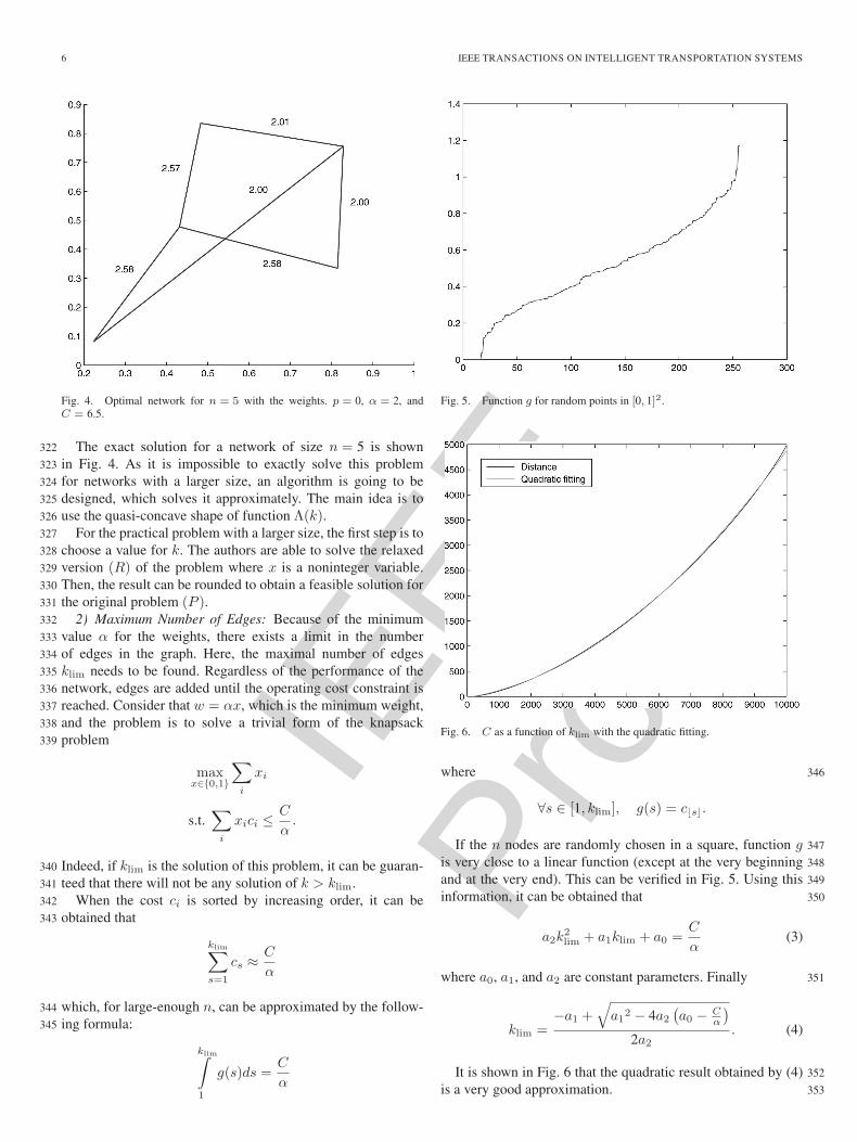
IEEE

Proo

f

6 IEEE TRANSACTIONS ON INTELLIGENT TRANSPORTATION SYSTEMS

Fig. 4. Optimal network for n = 5 with the weights. p = 0, α = 2, andC = 6.5.

The exact solution for a network of size n = 5 is shown322

in Fig. 4. As it is impossible to exactly solve this problem323

for networks with a larger size, an algorithm is going to be324

designed, which solves it approximately. The main idea is to325

use the quasi-concave shape of function Λ(k).326

For the practical problem with a larger size, the first step is to327

choose a value for k. The authors are able to solve the relaxed328

version (R) of the problem where x is a noninteger variable.329

Then, the result can be rounded to obtain a feasible solution for330

the original problem (P ).331

2) Maximum Number of Edges: Because of the minimum332

value α for the weights, there exists a limit in the number333

of edges in the graph. Here, the maximal number of edges334

klim needs to be found. Regardless of the performance of the335

network, edges are added until the operating cost constraint is336

reached. Consider that w = αx, which is the minimum weight,337

and the problem is to solve a trivial form of the knapsack338

problem339

maxx∈{0,1}

∑i

xi

s.t.∑i

xici ≤C

α.

Indeed, if klim is the solution of this problem, it can be guaran-340

teed that there will not be any solution of k > klim.341

When the cost ci is sorted by increasing order, it can be342

obtained that343

klim∑s=1

cs ≈C

α

which, for large-enough n, can be approximated by the follow-344

ing formula:345

klim∫1

g(s)ds =C

α

Fig. 5. Function g for random points in [0, 1]2.

Fig. 6. C as a function of klim with the quadratic fitting.

where 346

∀s ∈ [1, klim], g(s) = c�s .

If the n nodes are randomly chosen in a square, function g 347

is very close to a linear function (except at the very beginning 348

and at the very end). This can be verified in Fig. 5. Using this 349

information, it can be obtained that 350

a2k2lim + a1klim + a0 =

C

α(3)

where a0, a1, and a2 are constant parameters. Finally 351

klim =−a1 +

√a12 − 4a2

(a0 − C

α

)2a2

. (4)

It is shown in Fig. 6 that the quadratic result obtained by (4) 352

is a very good approximation. 353

IEEE

Proo

f

WEI et al.: ALGEBRAIC CONNECTIVITY MAXIMIZATION FOR AIR TRANSPORTATION NETWORKS 7

B. SDP Formulation354

To solve the larger size problem, the relaxation of the prob-355

lem is expressed as an SDP that will be solved efficiently. When356

v is not normalized, recall (1) in Property 1, which can be then357

transformed as358 {λ2 = maxλ λλvT v ≤ vTLv∀v ∈ R

n, vT e = 0.

Variable μ is added, which allows any v ∈ Rn359 {

λ2 = maxλ,μ λ∀v ∈ R

n, vT (μeeT )v + vTLv − λvT v ≥ 0.

It can be written using Loewner’s order [33]360 {λ2 = maxλ,μ λμeeT + L− λI 0.

(5)

The relaxation of the problem that needs to be solved is361

maxx,w,k

λ2 (L(w)) s.t.

⎧⎪⎨⎪⎩

∑i xi = k

xi ∈ [0, 1]∑i wici ≤ C

αxi ≤ wi ≤ βxi

which now becomes with (5)362

maxx,w,k,λ,μ

λ s.t.

⎧⎪⎪⎪⎨⎪⎪⎪⎩

∑i xi = k

xi ∈ [0, 1]∑i wici ≤ C

αxi ≤ wi ≤ βxi

μeeT + L− λI 0.

(6)

This problem is an SDP since there is a semidefinite constraint363

and all the other constraints are linear. It can be solved effi-364

ciently by an SDP solver. SeDuMi [34] is used in this paper.365

1) Optimality Conditions: The primal SDP is366

maxx,w,k,λ,μ

λ s.t.

⎧⎪⎪⎪⎨⎪⎪⎪⎩

∑i xi = k

xi ∈ [0, 1]∑i wici ≤ C

αxi ≤ wi ≤ βxi

μeeT + L− λI 0.

The variables are rescaled by dividing w, k, and x by λ and C.367

The dual SDP problem is368

minx,w,k,λ

∑i

wici s.t.

⎧⎪⎪⎨⎪⎪⎩

∑i xi = k

xi ∈ [0, 1]αxi ≤ wi ≤ βxi

L I − 1nJ

where J is the all-one matrix. When xij is relaxed (please see369

Section II-C), the relaxed dual SDP formulation is370

minx,w,k,λ

∑i

wici s.t.

{0 ≤ wi ≤ βL I − 1

nJ.

X is the matrix of the operating costs. The matrix format371

relaxed dual SDP is therefor372

maxX

⟨I − 1

nJ,X

⟩s.t.

{X 0〈E,X〉 = cij

where E is the matrix with Eii = Ejj = 1 and Eij=Eji=−1.373

Fig. 7. Upper bound: λ2 = f(k).

The Karush–Kuhn–Tucker optimality conditions are 374⎧⎪⎨⎪⎩

SX = XS = 0S 0, X 0〈E,X〉 = cijL− I + 1

nJ = S.

If wi = w for all i, it can be obtained that 375

S = (nw − 1)

(I − 1

nJ

).

When w = 1/n, S = 0 and the conditions are satisfied. 376

Reciprocally, if the optimality conditions are satisfied, it can 377

be obtained that 378(L−

(I − 1

nJ

))X = 0.

X has rank n; hence 379

L = I − 1nJ.

Thus, w is constant for all i and w = 1/n. 380

For edge i and edge j, the optimality condition is finally 381

obtained 382{∀(i, j), wi = wj∑

i wici = C.

2) Upper Bound: With the SDP formulation, the relaxation 383

can now be solved. When the values of the optimal connectivity 384

for different values of k are computed, the upper bound is 385

plotted in Fig. 7. 386

The relaxed problem reached its maximum for several values 387

of k contained in an interval [kmin, kmax]. Indeed, the optimal- 388

ity conditions give 389{∀(i, j), wi = wj∑m

i=1 wici = C.

All the weights are equal and their value is ∀i, wi = 390

(C/(∑

j cj)) = Ω. If w = βx, all the elements of x are equal 391

IEEE

Proo

f

8 IEEE TRANSACTIONS ON INTELLIGENT TRANSPORTATION SYSTEMS

and their value is ∀i, xi = (k/(n2 − n)), which leads to392

kmin =Ω(n2 − n)

β.

By doing the same computation, it is proved that the optimal393

value is also reached with394

kmax =Ω(n2 − n)

α

and ∀k ∈ [kmin, kmax], the optimal value is achieved.395

However, it needs to be pointed out that when the solution396

is rounded, infeasible solution may appear. For example, if k =397

kmin, there is often no solution since398 ∑i

xi =nΩ

β< n− 1

if (Ω/β) � 1, which is often the case. In addition, because at399

least n− 1 edges are needed to connect an n node graph, there400

is no positive solution. Therefor, the upper bound is not a very401

good bound for small values of k.402

C. Rounding Techniques for SDP Solution403

1) Description of the Methods: In this section, suppose that404

the relaxed optimal solution s0 has been found. k edges are405

going to be selected from s0, which means that xi = 1 for k406

values and xi = 0 for the others. There are several ways to do407

so. The methods that have been studied and implemented are408

listed.409

1) Greedy: Choose the k biggest elements s0(xi) in the re-410

laxed solution. Then, find the optimal weights by solving411

the corresponding SDP.412

2) Random fast: Randomly choose the rounding. For each413

i ∈ {1, . . . ,m}, xi = 1 with probability s0(xi) and xi =414

0 otherwise. Then, the weights are affected with the415

following value:416

s0(wi)

s0(xi).

These two steps are repeated many times. The average417

value xi of xi is s0(xi); therefor418 ∑i

xi =∑i

s0(xi) = k

and for the same reason419

∑i

wici =∑i

s0(wi)

s0(xi)xici =

∑i

s0(wi)ci ≤ C.

Thus, on average, the solution satisfies the constraints.420

At the end, keep the best solution that satisfies all the421

constraints.422

3) Random: In addition, randomly choose the rounding. If423 ∑i xi = k, which is the case on average, evaluate the424

weights by solving the SDP formulation. The steps are425

repeated several times, and keep the best value.426

Fig. 8. λ2 as a function of k. The results from several rounding methods arerepresented for a 20-node graph.

4) Step by step: Select the biggest element s0(xi) < 1 and 427

affect its value to 1 in the SDP formulation. Then, solve 428

the SDP again and repeat k times for these two steps. 429

5) Log step by step: This is the same idea as the “step by 430

step” except that, at each step, choose the best half of 431

the remaining elements. Thus, there are only log(k) SDPs 432

that have to be solved. 433

2) Numerical Results: The simulation is set up with 20 434

nodes randomly generated in a square. The results are presented 435

in Fig. 8 with λ2 as a function of k. The upper bound ob- 436

tained by the relaxation is plotted, as well as all the rounding 437

techniques. 438

It turns out that some techniques may fail to find a solution. In 439

this case, the corresponding values are removed from the figure. 440

It can be seen that the algorithms can achieve the upper 441

bound at the maximum number of edges klim. This shows that 442

any algorithm based on edge addition without considering the 443

variable weights is not adapted. 444

Pros and Cons: Each of the methods presented has some 445

advantages and drawbacks. The one that gives the best result is 446

the step-by-step method. The fastest is random fast. In addition, 447

the method that gives the best tradeoff between speed and value 448

is log step by step. 449

D. Relaxed SDP With Rounding Algorithm 450

This algorithm is used to solve relatively small-scale problem 451

when the exhaustive search described in Section III-A fails. 452

1) Golden Section Search: For a given k, a well-connected 453

network with k edges can now be found. Instead of testing all 454

the possible values of k, the search can be speeded up by con- 455

sidering that algebraic connectivity is a concave function of k. 456

This approximation leads to better results with rounding 457

methods that have good regularity. For large networks, the 458

rounding methods with lower regularity can be used. Instead 459

of computing the value for a given k, a local average value is 460

computed based on three values 461

∀k ∈ N, f̃(k) =f(k − 1) + f(k) + f(k + 1)

3.

As only the value of the connectivity for integer values 462

of k can be computed, it is not possible to use continuous 463

optimization principles. Thus, the golden section search [35] 464

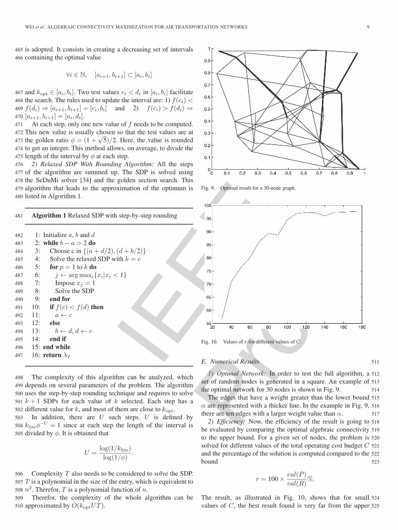
IEEE

Proo

f

WEI et al.: ALGEBRAIC CONNECTIVITY MAXIMIZATION FOR AIR TRANSPORTATION NETWORKS 9

is adopted. It consists in creating a decreasing set of intervals465

containing the optimal value466

∀i ∈ N, [ai+1, bi+1] ⊂ [ai, bi]

and kopt ∈ [ai, bi]. Two test values ci < di in [ai, bi] facilitate467

the search. The rules used to update the interval are: 1) f(ci) <468

f(di) ⇒ [ai+1, bi+1] = [ci, bi] and 2) f(ci) > f(di) ⇒469

[ai+1, bi+1] = [ai, di].470

At each step, only one new value of f needs to be computed.471

This new value is usually chosen so that the test values are at472

the golden ratio φ = (1 +√

5)/2. Here, the value is rounded473

to get an integer. This method allows, on average, to divide the474

length of the interval by φ at each step.475

2) Relaxed SDP With Rounding Algorithm: All the steps476

of the algorithm are summed up. The SDP is solved using477

the SeDuMi solver [34] and the golden section search. This478

algorithm that leads to the approximation of the optimum is479

listed in Algorithm 1.480

Algorithm 1 Relaxed SDP with step-by-step rounding481

1: Initialize a, b and d482

2: while b− a > 2 do483

3: Choose c in {(a+ d/2), (d+ b/2)}484

4: Solve the relaxed SDP with k = c485

5: for p = 1 to k do486

6: j ← argmaxi{xi|xi < 1}487

7: Impose xj = 1488

8: Solve the SDP489

9: end for490

10: if f(c) < f(d) then491

11: a ← c492

12: else493

13: b ← d, d ← c494

14: end if495

15: end while496

16: return λ2497

The complexity of this algorithm can be analyzed, which498

depends on several parameters of the problem. The algorithm499

uses the step-by-step rounding technique and requires to solve500

k + 1 SDPs for each value of k selected. Each step has a501

different value for k, and most of them are close to kopt.502

In addition, there are U such steps. U is defined by503

klimφ−U = 1 since at each step the length of the interval is504

divided by φ. It is obtained that505

U =log(1/klim)log(1/φ)

.

Complexity T also needs to be considered to solve the SDP.506

T is a polynomial in the size of the entry, which is equivalent to507

n2. Therefor, T is a polynomial function of n.508

Therefor, the complexity of the whole algorithm can be509

approximated by O(koptUT ).510

Fig. 9. Optimal result for a 30-node graph.

Fig. 10. Values of r for different values of C.

E. Numerical Results 511

1) Optimal Network: In order to test the full algorithm, a 512

set of random nodes is generated in a square. An example of 513

the optimal network for 30 nodes is shown in Fig. 9. 514

The edges that have a weight greater than the lower bound 515

α are represented with a thicker line. In the example in Fig. 9, 516

there are ten edges with a larger weight value than α. 517

2) Efficiency: Now, the efficiency of the result is going to 518

be evaluated by comparing the optimal algebraic connectivity 519

to the upper bound. For a given set of nodes, the problem is 520

solved for different values of the total operating cost budget C 521

and the percentage of the solution is computed compared to the 522

bound 523

r = 100 × val(P )

val(R)%.

The result, as illustrated in Fig. 10, shows that for small 524

values of C, the best result found is very far from the upper 525

IEEE

Proo

f

10 IEEE TRANSACTIONS ON INTELLIGENT TRANSPORTATION SYSTEMS

Fig. 11. Time (in seconds) to solve the SDP formulation of the problem for agiven number of n nodes.

bound. However, when increasing C, the objective value of the526

problem P quickly increases to reach the value of its relaxed527

problem R.528

IV. LARGE-SCALE AIR TRANSPORTATION NETWORKS529

A. Necessity530

The method in the previous section is going to be applied to531

large networks. The most time-consuming computation in the532

process is solving the SDP. Fig. 11 shows the computational533

time of solving one SDP for n nodes. It is observed that the534

running time increases very rapidly. In fact, for n nodes, there535

are n(n− 1) + 2 ∼ n2 variables in the SDP. As several SDPs536

need to be computed in order to solve the problem, it becomes537

impossible for n ≥ 35 on the authors’ workstation.538

However, it is necessary to get some results for large values539

of n because real networks are usually large. For example, the540

air transportation network contains several hundred nodes when541

considering the entire USA.542

B. Cluster Decomposition543

Since the key factor for operating cost for each link is the544

route distance (a longer distance route consumes more fuel), the545

idea in this section is to divide the airports into g ∈ N clusters546

based on the distance between the nodes. These clusters can be547

solved independently with the relaxed SDP method (Algorithm 1)548

developed in the previous section and can be connected549

afterward.550

To connect the cluster, choose k major nodes in each cluster551

that will be connected to each other. Then, the problem P has to552

be solved for these g × k nodes, except that links between two553

nodes from the same cluster are not allowed; hence, the graph554

is not complete.555

At the end, g + 1 problems of type (P ) need to be solved to556

get the final result. Fig. 12 shows the idea of the decomposition557

into several clusters and the selection of major nodes.558

Fig. 12. Set of 16 nodes separated in three clusters with two major nodes ineach cluster (in red).

There are several parameters whose values have to be chosen 559

to apply this idea. First, choose the number of clusters and how 560

many major nodes are used in each cluster to connect to other 561

clusters. Second, choose which nodes are kept as major nodes 562

among each cluster. Naturally, it is decided here to take the 563

airports that have the largest traffic demand. 564

In addition, to solve the problem for each small problem 1 ≤ 565

i ≤ g + 1, the value of the maximum operating cost budget Ci 566

in each cluster has to be chosen. A natural option is to choose 567

Ci proportional to the sum si of all the costs of the edges in the 568

cluster i and such that∑g+1

i=1 Ci = C 569

si =∑

(x,y)∈Ecxy,

Ci =si∑g+1j=1 sj

C.

The separation of the nodes into several clusters is made 570

by k-means algorithm [36]. This algorithm has the advantages 571

of being fast, easy to implement, and generally giving good 572

results. 573

To sum up the method described above, the full cluster 574

decomposition algorithm is listed in Algorithm 2. 575

Algorithm 2 Large-scale cluster decomposition 576

1: Initialize g, Ci 577

2: k-means algorithm gives g clusters 578

3: for p = 1 to g do 579

4: Solve the cluster problem (with Algorithm 1) 580

5: end for 581

6: Solve the major node problem (Algorithm 1) 582

7: Build the resulting network 583

8: return λ2(L) 584

C. Evaluation of Efficiency 585

The goal here is to show that if all g + 1 clusters are well 586

connected, the resulting graph is well connected too. This 587

depends on the values of some parameters that characterize how 588

each cluster is linked to the others. 589

g clusters are considered. Each cluster has n nodes and k 590

of its nodes are used to connect to other clusters. Let G be 591

the matrix of the graph and F be the vector defined by the 592

IEEE

Proo

f

WEI et al.: ALGEBRAIC CONNECTIVITY MAXIMIZATION FOR AIR TRANSPORTATION NETWORKS 11

Fig. 13. (a) λ2 = f(n); (b) λ2 = f(k); (c) λ2 = f(g).

expression below. If, for instance, g = 3, matrix G can be put593

into the following form:594

G =

⎛⎜⎜⎜⎜⎜⎜⎜⎜⎜⎜⎝

E 0 0 E 0 0A1 0 0 0 0 0 0

0 0 0 0 0 0E 0 0 E 0 00 0 0 A2 0 0 00 0 0 0 0 0E 0 0 E 0 00 0 0 0 0 0 A3

0 0 0 0 0 0

⎞⎟⎟⎟⎟⎟⎟⎟⎟⎟⎟⎠

F =

⎛⎜⎜⎜⎜⎜⎜⎜⎜⎜⎜⎜⎝

αeβeβe000

−αe−βe−βe

⎞⎟⎟⎟⎟⎟⎟⎟⎟⎟⎟⎟⎠

with the following notation. e is the all-one vector. α and β are595

constants that will be computed in the next paragraph. A1, A2,596

and A3 represent the adjacency matrices of the three clusters.597

E is a k × k matrix with all elements equal to 1.598

1) Fiedler Vector: The Fiedler vector is the vector solution599

of the minimization problem600

minx∈Rn

{xTLx|‖x‖ = 1, xe = 0

}.

It is known to be an indicator on how to split a graph into two601

smaller graphs. In fact, the nodes that have the same sign in this602

vector form a cut of the graph (see [37]).603

Here, the optimal cut will naturally be found between two604

clusters. Since some of the nodes play the same role, the Fiedler605

vector has a shape close to F where α and β are constants that606

need to be determined.607

This assumption has been verified by numerical experiments608

and it seems to be a very good approximation of the real Fiedler609

vector.610

2) Computing the Connectivity: Consider that the Fiedler611

vector has the form of F and matrices are full, which means612

all nondiagonal elements are equal to 1. The matrix products 613

give 614

λ2 =FTLF,

λ2 = 2kαX + 2(n− k)βY

with 615

X =α (n− 1 + k(g − 1))− (k − 1)α− (n− k)β + kα,

Y =β(n− 1)− kα− (n− k − 1)β.

It is also known that ‖F‖ = 1; thus 616

2kα2 + (2n− 2k)β2 = 1,

α =

√1 − (2n− 2k)β

2k.

Substitute α with this expression and β is given by the 617

d λ2

d β= 0. (7)

With a computation software package like Maple, this gives 618

us the expression of function f such that 619

λ2 = f(n, k, g).

3) Resulted Curves: By solving (7), the values of α, β, and 620

λ2 are obtained. The following figures have been obtained with 621

Maple. Among the three parameters k, g, and n, fix two of them 622

and let the third one vary to see its influence on connectivity. 623

Fig. 13 provides a clearer idea on how to choose the value 624

of each parameter. For example, connectivity is almost linear 625

regarding k but has a concave shape when represented as a 626

function of the number of clusters g. 627

There exists a tradeoff: If g is too large, kg will be too large to 628

be solved. On the contrary, if g is too small, each of the cluster 629

will have too many nodes to be solved. 630

4) Numerical Results: The data used are the 100 largest 631

cities in the United States. Fig. 14 shows the 100 biggest 632

cities without any link. The cluster decomposition is used to 633

divide these 100 cities into g = 5 groups. In each group, we 634

selected k = 5. The lower bound α = 2 and the upper bound 635

IEEE

Proo

f

12 IEEE TRANSACTIONS ON INTELLIGENT TRANSPORTATION SYSTEMS

Fig. 14. Shown are the 100 largest cities in the USA.

Fig. 15. Result for the 100 largest cities in the USA.

β = 10. The total running time is 317 s with MATLAB on our636

workstation. The algebraic connectivity that we have achieved637

is λ2 = 2.6.638

The optimal network found is illustrated in Fig. 15. The blue639

lines represent the edges inside each cluster and the red lines640

represent the edges that connect nodes from different clusters.641

In a real network, most airlines use spoke-hub planning, in642

which the regional airports are clustered and connected to their643

regional hub airport. Fig. 15 shows the same behavior that644

regional airports are clustered together. In a real network in the645

United States, the number of the major nodes k for each cluster646

is usually 1, which means that the hub airport is the only major647

node for its cluster. In a real network in Europe, the number of648

the major nodes k is usually bigger than 1. In fact, the number649

k in a European network is those hub airports in each country.650

For example, Air France has hubs at Paris and Lyon (k = 2)651

and Air Berlin has its hubs at Berlin, Düsseldorf, Hamburg, and652

Munich (k = 4). In summary, the result in Fig. 15 is a practical653

design, and more importantly, the computation is very efficient654

for large-scale network planning.655

V. DIRECTED AIR TRANSPORTATION NETWORK 656

A. From Undirected Graph to Directed Graph 657

In this section, the methods are extended in directed graphs. 658

In order to be consistent with the undirected case, the graphs 659

need to be balanced, which means that the number of aircraft 660

that comes in is the same as the number of aircraft that leaves 661

the airport 662

∀i ∈ {1, . . . , n},n∑

j=1

wij =n∑

k=1

wki.

It is clear that the set of undirected graphs is included in the set 663

of directed balanced graphs. Therefor, the results should be at 664

least as good as in the previous section. 665

Definition: According to [38], if Ω = {x ∈ Rn, xe = 666

0, ‖x‖ = 1}, the definition of the algebraic connectivity can be 667

extended for directed balanced graphs with 668

minx∈Ω

xTLx = λ2

(12(L+ LT )

).

Property 4: In the directed case and with this definition 669

of the algebraic connectivity, the upper bound given by the 670

continuous relaxation is the same as in the undirected case. 671

Proof: Given the optimum directed balanced graph in the 672

relaxed problem and its incidence matrix G, H can be created 673

H =G+GT

2

where H is symmetric and satisfies all the constraints of the 674

problem since they are linear. In addition with the definition of 675

the connectivity for directed graphs, the connectivity of H is 676

clearly the same as the connectivity of G. 677

Since it is also known that undirected graphs are a subset of 678

directed balanced graphs, the bounds are equal in both cases. 679

This will allow us to easily evaluate the improvement brought 680

by directed graphs. � 681

B. Results 682

The same method is used as in Section III. The results are 683

impressively better with directed graphs, as shown in Fig. 16. 684

The best value for the directed balanced case almost reached 685

the upper bound. It is also noticed that the optimal result has 686

less edges than the optimal network in the undirected case (an 687

edge in the undirected case is counted in both ways). 688

It is shown in Fig. 17 that most of the edges in the optimal 689

solution are oriented in only one way, which shows that the 690

solution is very different from the undirected case. 691

However, there is an important drawback. Indeed, two times 692

as many variables are needed for directed networks. Thus, the 693

problem takes a much longer time to be solved and is only 694

applicable on smaller networks. 695

IEEE

Proo

f

WEI et al.: ALGEBRAIC CONNECTIVITY MAXIMIZATION FOR AIR TRANSPORTATION NETWORKS 13

Fig. 16. λ = f(k) for the same graph with different approaches.

Fig. 17. Optimal directed graph.

C. Failure Case696

If an edge or a node is removed, the graph is not balanced697

anymore. This can cause important problems in practice; hence,698

the remaining weights in the graph need to be changed to handle699

this problem.700

This operation can be done by using a flow algorithm. The701

first step is to link the nodes with positive aircraft balance to a702

virtual source and those with negative balance to a sink. The ca-703

pacities of these links are equal to the absolute value of the704

difference in the balance flow for the node. The capacity of the705

other links of the graph is β.706

Then, consider the problem of the maximization of the flow707

from the source to the sink. This problem can be solved by using708

Edmonds–Karp algorithm [39], which has efficient complexity,709

i.e., O(nm2). This algorithm maintains the balance of the flow710

at each node.711

At the end, the graph is the graph solution of the flow712

problem when the source and the sink are removed. Figs. 18713

and 19 show an example of a graph in which a node is removed,714

Fig. 18. Example of a graph with a node failure.

Fig. 19. Example of a graph after maximization of the flow.

before and after maximization of the flow. The graph in Fig. 19 715

is now balanced by Edmonds–Karp algorithm after removing 716

the source (green node) and the sink (blue node). 717

VI. CONCLUSION 718

In this paper, a new problem concerning the maximization of 719

the algebraic connectivity of a network has been presented and 720

studied. This problem consists of finding both the edges of the 721

graph and their weight assignment under several constraints. 722

First, the problem in small networks is exactly solved, and it is 723

shown that the problem cannot be separated into two already 724

studied independent problems. Then, a relaxed SDP method 725

with step-by-step rounding is presented to solve the problem 726

approximately for better computational efficiency. With the 727

method developed for small-scale network, the cluster decom- 728

position method is proposed to solve the large-scale network 729

problem and successfully find the near-optimal solution for a 730

network of the 100 largest cities in the United States. Finally, 731

the study is extended to directed graphs. Numerical experiments 732

and analysis are performed for all the proposed algorithms. The 733

developed methods are able to model and maximize robustness 734

in air transportation networks for airlines and for the NAS. They 735

also provide an option to improve current ways of the generic 736

network design. 737

IEEE

Proo

f

14 IEEE TRANSACTIONS ON INTELLIGENT TRANSPORTATION SYSTEMS

REFERENCES738

[1] R. Guimera and L. Amaral, “Modeling the world-wide airport network,”739Eur. Phys. J. B, Condens. Matter Complex Syst., vol. 38, no. 2, pp. 381–740385, Mar. 2004.741

[2] R. Kincaid, N. Alexandrov, and M. Holroyd, “An investigation of syn-742chrony in transport networks,” Complexity, vol. 14, no. 4, pp. 34–43,743Mar./Apr. 2008.744

[3] E. Vargo, R. Kincaid, and N. Alexandrov, “Towards optimal transport745networks,” J. Syst., Cybern. Inf., vol. 8, no. 4, pp. 59–64, Jul. 2010.746

[4] International Civil Aviation Organization (ICAO), “Procedures for air747navigation services—Rules of the air and air traffic services,” Montréal,748QC, Canada, doc 4444-RAC/501, 2010.749

[5] P. Kostiuk, D. Lee, and D. Long, “Closed loop forecasting of air traffic750demand and delay,” presented at the 3rd USA/Europe Air Traffic Man-751agement R&D Seminar, Napoli, Italy, Jun. 2010, Paper 80.752

[6] K. Nam and T. Schaefer, “Forecasting international airline passenger753traffic using neural networks,” Logist. Transp. Rev., vol. 31, no. 3, pp. 239–754251, Sep. 1995.755

[7] F. Alamdari and S. Fagan, “Impact of the adherence to the original low756cost model on the profitability of low cost airlines,” Transp. Rev., vol. 25,757no. 3, pp. 377–392, May 2005.758

[8] M. Dresner, J.-S. C. Lin, and R. Windle, “The impact of low-cost carriers759on airport and route competition,” J. Transp. Econ. Policy, vol. 30, no. 3,760pp. 309–328, Sep. 1996.761

[9] K. Button and S. Lall, “The economics of being an airport hub city,” Res.762Transp. Econ., vol. 5, pp. 75–105, 1999.763

[10] T. Oum, A. Zhang, and Y. Zhang, “A note on optimal airport pricing in a764hub-and-spoke system,” Transp. Res. B, Methodol., vol. 30, no. 1, pp. 11–76518, Feb. 1996.766

[11] X.-B. Hu, W.-H. Chen, and E. Di Paolo, “Multiairport capacity man-767agement: Genetic algorithm with receding horizon,” IEEE Trans. Intell.768Transp. Syst., vol. 8, no. 2, pp. 254–263, Jun. 2007.769

[12] X.-B. Hu and E. Di Paolo, “Binary-representation-based genetic algo-770rithm for aircraft arrival sequencing and scheduling,” IEEE Trans. Intell.771Transp. Syst., vol. 9, no. 2, pp. 301–310, Jun. 2008.772

[13] Y. Eun, I. Hwang, and H. Bang, “Optimal arrival flight sequencing and773scheduling using discrete airborne delays,” IEEE Trans. Intell. Transp.774Syst., vol. 11, no. 2, pp. 359–373, Jun. 2010.775

[14] Z.-H. Zhan, J. Zhang, Y. Li, O. Liu, S. Kwok, W. Ip, and O. Kaynak,776“An efficient ant colony system based on receding horizon control for the777aircraft arrival sequencing and scheduling problem,” IEEE Trans. Intell.778Transp. Syst., vol. 11, no. 2, pp. 399–412, Jun. 2010.779

[15] FlightStats-Global Flight Tracker, Status Tracking and Airport Informa-780tion, FlightStats, Inc., Portland, OR, USA, 2013, retrieved on March 16,7812013. [Online]. Available: http://www.flightstats.com782

[16] Federal Aviation Administration (FAA), “FAA Aerospace Forecasts FY7832008-2025,” Washington, DC, USA, Dec. 2010.784

[17] S. Conway, “Scale-free networks and commercial air carrier transporta-785tion in the United States,” in Proc. 24th Int. Congr. Aeron. Sci., Yokohama,786Japan, 2004, pp. 1–12.787

[18] P. A. Bonnefoy, “Scalability of the air transportation system and develop-788ment of multi-airport systems: A worldwide perspective,” Ph.D. disserta-789tion, MIT, Cambridge, MA, USA, Jun. 2008.790

[19] N. Alexandrov, “Transportation network topologies,” NASA Langley Res.791Center, Hampton, VA, USA, Tech. Rep., 2004.792

[20] T. Kotegawa, D. DeLaurentis, K. Noonan, and J. Post, “Impact of com-793mercial airline network evolution on the US air transportation system,” in794Proc. 9th USA/Europe ATM Res. Develop. Semin., Berlin, Germany, 2011.AQ3 795

[21] A. Bigdeli, A. Tizghadam, and A. Leon-Garcia, “Comparison of network796criticality, algebraic connectivity, and other graph metrics,” presented at797the 1st Annu. Workshop Simplifying Complex Network Practitioners,798Venice, Italy, 2009, Paper 4.799

[22] A. Jamakovic and S. Uhlig, “On the relationship between the algebraic800connectivity and graph’s robustness to node and link failures,” in Proc.8013rd EuroNGI Netw. Conf., May 2007, pp. 96–102.802

[23] A. Jamakovic and P. V. Mieghem, “On the robustness of complex net-803works by using the algebraic connectivity,” in Proc. Netw. Ad Hoc Sen-804sor Netw., Wireless Netw., Next Gen. Internet, A. Das, H. K. Pung,805F. Bu Sung Lee, and L. Wong Wai Choong, Eds., 2008, pp. 183–194.806

[24] R. H. Byrne, J. T. Feddema, and C. T. Abdallah, “Algebraic connectivity807and graph robustness,” Sandia Nat. Lab., Albuquerque, NM, USA, Tech.808Rep., Jul. 2009.809

[25] P. Wei and D. Sun, “Weighted algebraic connectivity: An application810to airport transportation network,” in Proc. 18th IFAC World Congress,811Milan, Italy, Aug. 2011, pp. 13 864–13 869.812

[26] A. Ghosh and S. Boyd, “Growing well-connected graphs,” in Proc. 45th813IEEE Conf. Decis. Control, Dec. 2006, pp. 6605–6611.814

[27] J. Sun, S. Boyd, L. Xiao, and P. Diaconis, “The fastest mixing Markov 815process on a graph and a connection to a maximum variance unfolding 816problem,” SIAM Rev., vol. 48, no. 4, pp. 681–699, Nov. 2006. 817

[28] F. Goring, C. Helmberg, and M. Wappler, “Embedded in the shadow of 818the separator,” SIAM J. Optim., vol. 19, no. 1, pp. 472–501, Feb. 2008. 819

[29] S. Boyd, “Convex optimization of graph Laplacian eigenvalues,” in Proc. 820Int. Congr. Math., 2006, vol. 3, pp. 1311–1319. 821

[30] S. Boyd, P. Diaconis, and L. Xiao, “Fastest mixing Markov chain on a 822graph,” SIAM Rev., vol. 46, no. 4, pp. 667–689, Dec. 2004. 823

[31] M. Fiedler, “Algebraic connectivity of graphs,” Czechoslovak Math. J., 824vol. 23, no. 98, pp. 298–305, 1973. 825

[32] B. Mohar, “The Laplacian spectrum of graphs,” in Graph Theory, 826Combinatorics, and Applications. New York, NY, USA: Wiley, 1991, 827pp. 871–898. 828

[33] M. Siotani, “Some applications of Loewner’s ordering on symmetric ma- 829trices,” Ann. Inst. Stat. Math., vol. 19, no. 1, pp. 245–259, Dec. 1967. 830

[34] J. F. Sturm, “Using SeDuMi 1.02, A Matlab toolbox for optimization over 831symmetric cones,” Optim. Methods Softw., vol. 11, no. 1–4, pp. 625–653, 832Jan. 1999. 833

[35] W. Press, S. Teukolsky, W. Vetterling, and B. Flannery, The Art of Scien- 834tific Computing, 3rd ed. Cambridge, U.K.: Cambridge Univ. Press, 2007. 835ch. Section 10.2. Golden Section Search in One Dimension, pp. 492–496. 836

[36] J. Kleinberg and E. Tardos, Algorithm Design. Reading, MA, USA: 837Addison-Wesley, 2005, ch. 4.7 Clustering, pp. 157–161. 838

[37] S. Martinez, G. Chatterji, D. Sun, and A. Bayen, “A weighted graph ap- 839proach for dynamic airspace configuration,” presented at the AIAA Conf. 840Guidance, Control Dynamics, Hilton Head, SC, USA, Aug. 2007, Paper 841AIAA 2007-6448. 842

[38] C. Wu, “Algebraic connectivity of directed graphs,” Linear Multilinear 843Algebra, vol. 53, no. 3, pp. 203–223, Jun. 2005. 844

[39] T. H. Cormen, C. E. Leiserson, R. L. Rivest, and C. Stein, Introduction 845to Algorithms. Cambridge, MA, USA: MIT Press, 2009, ch. 26.2 The 846Ford-Fulkerson method, pp. 727–730. 847

Peng Wei (M’12) received the Bachelor’s degree 848in automation from Tsinghua University, Beijing, 849China; the Master’s degree in electrical engineering 850from Stony Brook University, Stony Brook, NY, 851USA; and the Ph.D. degree in aerospace engineering 852from Purdue University, West Lafayette, IN, USA. 853

He is an Operations Research Consultant with 854American Airlines, Fort Worth, TX, USA. His re- 855search interests include next-generation air trans- 856portation system, environmental impact of aviation, 857and unmanned aerial vehicle integration in the Na- 858

tional Airspace System. 859Dr. Wei received the Purdue College of Engineering Outstanding Research 860

Award in 2013. 861

Gregoire Spiers received the Bachelor’s degree 862in applied mathematics from École Polytechnique, 863Palaiseau, France, in 2012. 864

He was a Visiting Student with Purdue University, 865West Lafayette, IN, USA, in 2011. He is currently 866a Research Engineer with Amadeus S.A.S., Sophia 867Antipolis, France. AQ4868

Dengfeng Sun (M’08) received the Bachelor’s de- 869gree in precision instruments and mechanology from 870Tsinghua University, Beijing, China; the Master’s 871degree in industrial and systems engineering from 872The Ohio State University, Columbus, OH, USA; 873and the Ph.D. degree in civil engineering from Uni- 874versity of California, Berkeley, CA, USA. 875

He is an Assistant Professor with the School of 876Aeronautics and Astronautics, Purdue University, 877West Lafayette, IN, USA. His research interests in- 878clude control and optimization, with an emphasis on 879

applications in air traffic flow management, dynamic airspace configuration, 880and studies for the next-generation air transportation system. 881

IEEE

Proo

f

AUTHOR QUERIES

AUTHOR PLEASE ANSWER ALL QUERIES

AQ1 = Please provide keywords.AQ2 = Please check if changes made in the affiliation note of author Gregoire Spiers are appropriate, with

reference to the given biography. Please also check accuracy of postal code and location.AQ3 = Please provide page range in Ref. [20].AQ4 = Please check accuracy of provided location.

END OF ALL QUERIES