ieee transactions on power systems 1 statistical …

IEEE P

roof

IEEE TRANSACTIONS ON POWER SYSTEMS 1

Statistical Modeling of Networked Solar Resourcesfor Assessing and Mitigating Risk of Interdependent

Inverter Tripping Events in Distribution Grids

1

2

3

Kaveh Dehghanpour , Member, IEEE, Yuxuan Yuan, Student Member, IEEE, Fankun Bu , Student Member, IEEE,and Zhaoyu Wang , Member, IEEE

4

5

Abstract—It is speculated that higher penetration of inverter-6based distributed photo-voltaic (PV) power generators can increase7the risk of tripping events due to voltage fluctuations. To quantify8this risk utilities need to solve the interactive equations of tripping9events for networked PVs in real-time. However, these equations10are non-differentiable, nonlinear, and exponentially complex, and11thus, cannot be used as a tractable basis for solar curtailment12prediction and mitigation. Furthermore, load/PV power values13might not be available in real-time due to limited grid observ-14ability, which further complicates tripping event prediction. To15address these challenges, we have employed Chebyshev’s inequality16to obtain an alternative probabilistic model for quantifying the17risk of tripping for networked PVs. The proposed model enables18operators to estimate the probability of interdependent inverter19tripping events using only PV/load statistics and in a scalable20manner. Furthermore, by integrating this probabilistic model into21an optimization framework, countermeasures are designed to mit-22igate massive interdependent tripping events. Since the proposed23model is parameterized using only the statistical characteristics of24nodal active/reactive powers, it is especially beneficial in practical25systems, which have limited real-time observability. Numerical26experiments have been performed employing real data and feeder27models to verify the performance of the proposed technique.

Q1

28

Index Terms—Probabilistic modeling, power statistics, risk29assessment, tripping events.30

I. INTRODUCTION31

INCREASING penetration of distributed energy resources32

(DERs), including inverter-based photo-voltaic (PV) power33

generators, in distribution grids represents opportunities for34

enhancing system resilience and customer self-sufficiency, as35

well as challenges in grid control and operation. One of these36

challenges is the potential increase in the risk of tripping of37

inverter-based resources due to undesirable fluctuations in the38

grid’s voltage profile [1]. This can put a hard limit on the feasible39

Manuscript received August 3, 2019; revised November 29, 2019 and January27, 2020; accepted February 9, 2020. This work was supported in part by theAdvanced Grid Modeling Program at the U.S. Department of Energy Officeof Electricity under Grant DE-OE0000875, and in part by the National Sci-ence Foundation under Grant ECCS 1929975. Paper no. TPWRS-01138-2019.(Corresponding author: Zhaoyu Wang.)

The authors are with the Department of Electrical and Computer Engineering,Iowa State University, Ames, IA 50011 USA (e-mail: [email protected];[email protected]; [email protected]; [email protected]).

Color versions of one or more of the figures in this article are available onlineat http://ieeexplore.ieee.org.

Digital Object Identifier 10.1109/TPWRS.2020.2973380

capacity of operational PVs in distribution grids, reduce the 40

economic value of renewable resources for customers, and cause 41

loss of service in stand-alone systems [2], [3]. The possibility 42

of DER power generation disruption due to voltage-related vul- 43

nerabilities in unbalanced distribution grids has been discussed 44

in the literature: in [4], [5], risk of interdependent tripping of 45

PVs, with ON/OFF current interruption mechanism was demon- 46

strated numerically in a distribution grid test case for the first 47

time. It was shown that the unbalanced and resistive nature of 48

networks can further exacerbate this problem by causing positive 49

inter-phase voltage sensitivity terms that act as destabilizing 50

positive feedback loops, leading to voltage deviations after 51

tripping of an individual inverter. The impact of grid voltage 52

sensitivity on DER curtailment was also studied and observed 53

in [2]. Based on these insights, guidelines were provided in [6] to 54

roughly estimate the impact of new DER capacity connections 55

on the maximum voltage deviations in the grid. It was shown 56

in [7] that very large or small number of inverter-based resources 57

in distribution systems can lead to interdependent failure events 58

that contribute to voltage collapse in transmission level. Detailed 59

realistic numerical studies were performed on practical feeder 60

models in [8]–[13] that corroborated the considerable impacts 61

of extreme PV integration levels, and inverter control modes on 62

grid voltage fluctuations, which is the critical factor in causing 63

massive solar curtailment scenarios. 64

Most existing works relied on scenario-based simulations and 65

numerical studies to capture the likelihood of inverter tripping 66

under high renewable penetration. While this has led to useful 67

guidelines and invaluable intuitions, it falls short of providing a 68

generic theoretical foundation for predicting and containing trip- 69

ping events. Specifically, the dependencies between nodal solar 70

power distributions, nodal voltage profiles, and inverter tripping 71

events have not been explicitly analyzed in the literature thus 72

far. These dependencies are influenced by inverter protection 73

settings and governed by a set of networked power-flow-based 74

equations, which turn out to be non-differentiable and nonlinear. 75

In this regard, several fundamental challenges have not been 76

addressed: (1) Lack of scalability: Solving the inverter tripping 77

equations directly in real-time requires a large-scale search pro- 78

cess to explore almost all the joint combinations of “ON/OFF” 79

configurations for the inverters. The computational complex- 80

ity is due to the interactive and networked nature of tripping 81

events, meaning that the states of inverters influence each other 82

0885-8950 © 2020 IEEE. Personal use is permitted, but republication/redistribution requires IEEE permission.See https://www.ieee.org/publications/rights/index.html for more information.

https://orcid.org/0000-0002-2701-6817

https://orcid.org/0000-0002-0007-5163

https://orcid.org/0000-0003-0656-0562

mailto:[email protected]




http://ieeexplore.ieee.org

IEEE P

roof

2 IEEE TRANSACTIONS ON POWER SYSTEMS

and are not independent [14]. The source of interdependency83

in chances of inverter tripping is the dependencies in nodal84

voltages of power grid (i.e., disruption of power injection at85

one node impacts nodal voltages of other neighboring inverters,86

which in turn could influence their probability of tripping.)87

For example, tripping of an inverter (or a cluster of inverters)88

leads to a change in loading distributions, which can most89

likely increase/decrease the chance of tripping for other inverters90

during under/over-voltage scenarios, especially in weak grids.91

This interdependency prevents the solver from decoupling the92

tripping equations into separate equations for individual invert-93

ers. Thus, the scale of search for finding the correct configuration94

increases exponentially (2N ) with the number of inverters (N ).95

Another factor that contributes to computational complexity is96

the volatility of PV power, which forces the solver to explore,97

not only various tripping configurations, but also numerous98

solar scenarios at granular time steps. (2) Limited tractability99

for mitigation: A direct solution strategy for tripping equations100

cannot be easily integrated into optimization-based decision101

models, since it has no predictive capability and cannot be use102

to answer what if queries, unless a thorough expensive search103

is performed over all possible future load/PV scenarios. Also,104

due to their non-differntiability, integrating the tripping equa-105

tions into decision models complicates formulation by adding106

integer variables to the problem. (3) Limited access to online107

data: Practical distribution grids have low online observability,108

meaning that the values of real-time nodal power injections can109

be unknown in real-time for a large number of PVs/loads due110

to communication time delays or limited number of sensors.111

Thus, we might not have access to sufficient online information112

to solve the tripping problem directly.113

To tackle these challenges, we propose an alternative prob-114

abilistic modeling approach to quantify and mitigate the risk115

of voltage-driven tripping events. Instead of complex scenario-116

based look-ahead search over numerous possible tripping117

configurations, our methodology is built upon probabilistic ma-118

nipulation of power flow equations in radial networks to estimate119

the probability of inverter tripping using only the available statis-120

tical properties of loads/PVs. Interdependent Bernoulli random121

variables are used to model probabilities of inverter tripping and122

capture their mutua. These probabilities are voltage-dependent123

and serve as unknown micro-states in the equations of tripping124

events. Then, Chebyshev’s inequality [15] is applied to deter-125

mine a stationary lower bound for the values that these micro-126

states can assume under any probable nodal power injection127

scenarios. This lower bound provides a conservative estimation128

of expected PV curtailment, and thus, represents a statistical risk129

metric for tripping events. Furthermore, due to its simple matrix-130

form and differentiable structure, the proposed probabilistic131

model can be conveniently integrated into an optimization132

framework as a constraint, which enables mitigating unwanted133

solar curtailment events by designing optimal voltage regulation134

countermeasures. The proposed methodology is generic and135

can capture the behavior of arbitrary radial distribution feeders136

using only load/PV statistics and network topology/parameters.137

This implies that tripping events can be conservatively predicted138

using the proposed model and without the need for online139

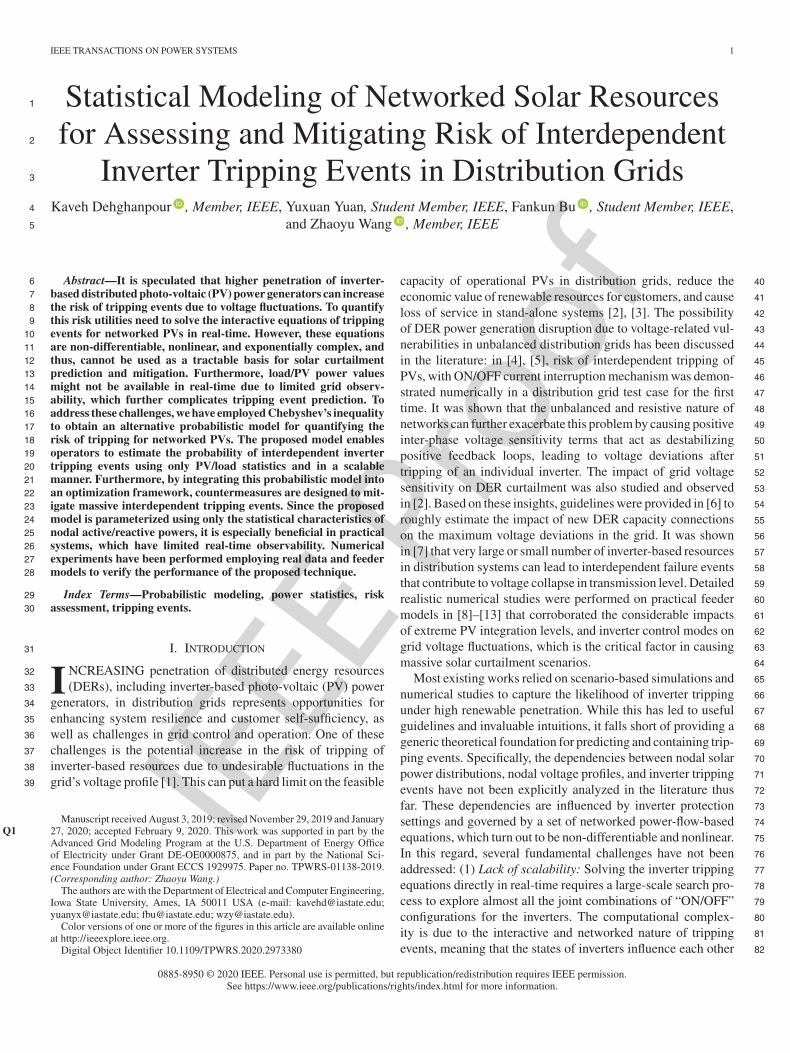
Fig. 1. Distribution feeder structure with PVs, loads, and voltage-sensitivecurrent interruption mechanisms (i.e., switches).

access to granular PV/load data or expensive scenario-based 140

search process, which makes our strategy specifically suitable 141

for practical networks. 142

Numerical experiments have been performed using real ad- 143

vanced metering infrastructure (AMI) data and feeder models 144

from our utility partners to validate the developed probabilistic 145

framework. The numerical validates the performance of the 146

probabilistic model for both over- and under-voltage scenarios, 147

and show that ignoring the possibility of tripping in voltage 148

regulation can exacerbate voltage deviations. 149

II. DERIVING A CONSERVATIVE PROBABILISTIC MODEL 150

OF PV TRIPPING EVENTS 151

In this section, we will develop and then parameterize a 152

probabilistic model of networked inverter-based PVs to quantify 153

the possibility of emergent tripping events. To do this, first, we 154

begin with the original model of inverter tripping with ON/OFF 155

voltage-driven current interruption mechanism, and then, we 156

will show that by adopting a probabilistic approach towards 157

the original model and using Chebyshev’s inequality, tripping 158

probabilities can be conservatively estimated using the statistical 159

properties of nodal available load/PV power. 160

A. Original Interactive Switching Equations 161

In this paper, it is assumed that PV resources are protected 162

against voltage deviations using ON/OFF switching mecha- 163

nisms. Note that here a “switch” can be a mechanical relay, 164

as well as a non-physical inverter control function that stops 165

current injection into the grid under abnormal voltage even 166

if the inverter is still physically connected to the grid [16]. 167

The PV is tripped in case the nodal voltage deviates from a 168

user-defined permissible range, [Vmin, Vmax]. In this paper, this 169

range is adopted from the literature [4], as Vmin = 0.9 p.u. 170

and Vmax = 1.1 p.u.. The switching mechanisms are simply 171

modelled as binary micro-state variables with the following 172

voltage-dependent function (see Fig. 1): 173

si(t) =

⎧⎪⎨

⎪⎩

1 Vmin ≤ Vi(t) ≤ Vmax

0 Vi(t) < Vmin

0 Vi(t) > Vmax

(1)

where, si(t) is the micro-state assigned to the i’th PV at time 174

t as a function of the inverter node’s voltage magnitude Vi. 175

IEEE P

roof

DEHGHANPOUR et al.: STATISTICAL MODELING OF NETWORKED SOLAR RESOURCES FOR ASSESSING AND MITIGATING RISK 3

Here, si(t) = 1 implies ON and si(t) = 0 indicates OFF. The176

assumption in this switching model is that over long enough177

time intervals the impact of inverter dynamics, e.g., ride-through178

capabilities [17]–[20], can be conservatively ignored. This as-179

sumption considerably enhances the tractability of the model180

at the expense of loss of accuracy. In this sense, the switching181

model is a worst-case representation of inverter tripping. Since182

the approximate power flow equations for distribution grids183

are linear with respect to the squared values of nodal voltage184

magnitudes [21], we re-write equation (1) using a variable185

transformation, vi = V 2i , and employing unit step functions as186

follows:187

si(t) = U(vi(t)− vmin)− U(vi(t)− vmax) (2)

where, vmin = V 2min, vmax = V 2

max, and the unit step function188

U(·) is defined as follows:189

U(x) =

{1 x ≥ 0

0 x < 0,(3)

Note that inverters’ micro-states are influenced by nodal190

voltages and are thus highly interdependent on each other, as191

changes in the state of one switch will cause nodal power192

variations, which leads to a change of voltage at other nodes193

that can in turn influence probability of tripping events. To194

obtain the overall governing equations of inverter tripping, the195

mutual impacts of switch micro-states on each other are captured196

using an approximate unbalanced power flow model for radial197

distribution grids [21], which determines voltage at node i as a198

function of active/reactive power injections of every other node199

in a grid (with a total of N + 1 nodes):200

vi(t) =N∑

j=1

vij + v0, ∀i ∈ {1, . . ., N} (4)

where, v0 = V 20 , with V0 denoting the voltage magnitude at a201

grid reference bus, and the intermediary variable vij represents202

the impact of active/reactive power injection at node j on vi,203

which is obtained as follows:204

vij = Rij pj(t) +Xij qj(t) (5)

where, Rij and Xij are the aggregated series resistance and205

reactance values corresponding to the intersecting branches in206

the paths connecting nodes i and j to the reference bus calculated207

as follows [21]:208

Rij = 2∑

{n,m}∈Pa(i,j)

rnm (6)

Xij = 2∑

{n,m}∈Pa(i,j)

xnm (7)

where,Pa(i, j) represents the set of pairwise nodes consisting of209

the neighboring nodes that are on the intersection of the unique210

paths connecting nodes i and j to the reference bus; rnm and211

xnm denote the real series resistance and reactance of the branch212

connecting nodes n and m. Also, pj and qj denote the active and213

reactive power injections at bus j, which are in turn determined214

by the micro-state of the PV at node j (see Fig. 1): 215

pj(t) = pj(t)sj(t) (8)

qj(t) = qj(t)sj(t) (9)

with pj and qj representing the available load/PV power at 216

node j, where pj > 0 implies generation. Equations (4)–(7) 217

are obtained in vector form for all three phases of unbalanced 218

distribution grids [21]. 219

Equations (2)–(9) fully determine the states of networked 220

PVs. The difficulty in solving these equations is due to three 221

factors: (I) the size of solution space increases exponentially 222

as the number of micro-states {s1, . . ., sN} grows. Since these 223

micro-states are not independent and influence each other in 224

complex and non-trivial ways they cannot be obtained individu- 225

ally, and a thorough search process is needed to explore all pos- 226

sible switching configurations. This can be extremely expensive 227

and impossible to scale to large systems with high population of 228

inverters. (II) Due to the discrete step functions in (2), tripping 229

equations are nonlinear and non-differentiable. This contributes 230

to problem difficulty since gradient-based methods cannot be ap- 231

plied. (III) pj and qj act as time-varying input parameters within 232

the model. This implies that using the tripping equations for pre- 233

dicting probability of tripping events requires extensive search 234

process to cover all probable PV/load time-series scenarios. This 235

expensive search process hinders the tractability of optimization- 236

based frameworks for designing tripping mitigation strategy. 237

Not all the nodes in the tripping model are necessarily con- 238

trolled by ON/OFF voltage-sensitive switching mechanisms. 239

For examples, ordinary load nodes are generally not governed 240

by equation (2). In this paper, for the sake of brevity, the 241

switching equations are still written for all the nodes in the grid 242

as presented, however, we will simply assign constant values, 243

si(t) = 1, ∀t to the nodes without ON/OFF control and remove 244

their corresponding switching from the equations (see Fig. 1). 245

B. Alternative Approximate Probabilistic Model 246

We adopt a probabilistic point of view towards tripping model. 247

This allows us to obtain a stationary differentiable statistical 248

model that has a simple matrix-form formulation. Accord- 249

ingly, the ON/OFF current interruption mechanisms, si’s, are 250

modelled as random variables following Bernoulli probability 251

distributions with parameters λi, ∀i ∈ {1, . . ., N}: si ∼ B(λi), 252

where parameter λi is defined as the probability of the i’th 253

inverter switch being ON, λi(t) = Pr{si(t) = 1}. The goal is 254

to transform micro-states from discontinuous binary variables 255

(si ∈ {0, 1}) into continuous variables (λi ∈ [0, 1]). To rewrite 256

the equations in terms of new micro-states note that we have 257

E{si(t)} = λi(t) for Bernoulli probability distributions, where 258

E{·} represents the expectation operation. Thus, by performing 259

an expectation operation over both sides of (2), probability of 260

inverter tripping in terms of the new micro-states can be obtained 261

as follows: 262

λi(t) = Pr {vmin ≤ vi(t) ≤ vmax} (10)

where, we have exploitedE{U(f(x))} = Pr{f(x) ≥ 0}. Note 263

that the probability of tripping for an inverter is an implicit 264

IEEE P

roof


function of nodal voltage probability distribution, which in265

turn is influenced by the states of other inverters. Due to the266

interconnected nature of the problem, no independency assump-267

tions has been made on random variables λi, ∀i ∈ {1, . . ., N}.268

However, the exact distributions of nodal voltages are unknown269

and complex functions of nodal active/reactive injections, which270

implies that (10) cannot be determined analytically unless over-271

simplifying assumptions are made. Instead, we employ Cheby-272

shev’s inequality [15] to provide a lower bound on micro-state273

as a function of nodal voltage statistics without making any274

assumption on voltage distributions,275

Pr{vmin ≤ vi(t) ≤ vmax} ≥ 1− σ2vi+(μvi

− vmax+vmin

2

)2

(vmax−vmin

2

)2

(11)where, σ2

viand μvi

are the variance and mean of vi, respectively.276

Hence, the approximate probabilistic model can be formulated277

for each micro-state as follows:278

λi(t) = 1− σ2vi+(μvi

− vmax+vmin

2

)2

(vmax−vmin

2

)2 (12)

This new tripping model has two features: (1) it is a conserva-279

tive estimator of the original system since it over-estimates the280

probability of inverter tripping, λi ≤ λi. (2) As will be shown in281

Section II-C, the approximate probabilistic model can be conve-282

niently parameterized in terms of nodal available active/reactive283

power statistics. Hence, as long as certain statistics are known (or284

estimated), the model allows us to accurately track probability of285

inverter tripping without running time-series simulations under286

numerous scenarios.287

C. Probabilistic Model Parameterization288

To parameterize the alternative tripping model (12), nodal289

voltage statistics, σ2vi

and μvi, are obtained in terms of nodal290

available active/reactive power statistics. To do this, power291

flow/injection equations (4)-(9) are leveraged.292

Stage 1: μviParameterization - The expected value of293

voltage magnitude squared is determined using (4)-(5) as,294

μvi=

N∑

j=1

E{vij}+ v0

=

N∑

j=1

(RijE{pj}+XijE{qj}) + v0 (13)

To calculate E{pj} and E{qj}, we will first obtain their295

cumulative distribution functions (CDFs) [15], Fpjand Fqj ,296

respectively. This process is shown for pj as follows (Fqj is297

obtained similarly):298

Fpj(P ) = Pr {pj(t) ≤ P} = (1−λj(t))U(P ) + λj(t)Fpj

(P )(14)

The rational behind (14) is that the distribution of power299

injection is determined by two functions: the distribution of PV300

switch (which is ON with probability λj(t)), and the CDF of301

available PV power, Fpj. Now, the probability density functions302

(PDF) of the realized active nodal power injection, fpj, can be303

calculated as a function of the available active solar power, fpj304

(a similar operation is performed for reactive power): 305

fpj(P ) =

dFpj(P )

dP= (1− λj(t))δ(P ) + λj(t)fpj

(P ) (15)

Then, using the active/reactive power injection PDFs, E{pj} 306

and E{qj}, can be obtained through integration: 307

E{pj} =

∫ +∞

−∞αfpj

(α)dα = λjPj (16)

E{qj} =

∫ +∞

−∞βfqj (β)dβ = λjQj (17)

where, Pj and Qj denote the mean values of the available active 308

and reactive powers at node j, respectively (Pj = E{pj} and 309

Qj = E{qj}). Thus, the mean nodal voltage magnitude squared 310

can be written in terms of inverter switch statistics and expected 311

PV/load available powers: 312

μvi=

N∑

j=1

{Rijλj(t)Pj +Xijλj(t)Qj}+ v0 (18)

Stage 2: σ2vi

Parameterization - Using (4), the variance of 313

nodal voltage magnitude squared can be formulated as, 314

σ2vi

=

N∑

j=1

σ2vij

+ 2∑

1≤k<j≤N

Ω {vij , vik} (19)

where, σ2vij

is the variance of vij , and the operator Ω{x1, x2} 315

denotes the covariance of the two random variables x1 and 316

x2, which itself can be written in terms of their correlation, 317

ρx1,x2, and standard deviations, σx1

and σx2, as Ω{x1, x2} = 318

ρx1,x2σx1

σx2. To fully parameterizeσ2

viusing available load/PV 319

power statistics, σ2vij

and Ω{vij , vik} have to be determined 320

separately. 321

Stage 2-1: σ2vij

Parameterization - Using (5), σ2vij

is formu- 322

lated as a function of pj and qj statistics: 323

σ2vij

= R2ijσ

2pj

+X2ijσ

2qj

+ 2RijXijΩ{pj , qj} (20)

where, σ2pj

and σ2qj

are the active/reactive power injection vari- 324

ances, which can in turn be determined as follows: 325

σ2pj

= E{s2jp

2j

}− E {pj}2 (21)

where,E{s2jp2j} is calculated through a similar process involved 326

in (14)-(17) (i.e., obtain the CDF, determine the PDF, and 327

integrate). Noting that in our case s2j = sj , the PDF of s2jp2j 328

is derived as follows (similar derivation applies to s2jq2j ): 329

fs2jp2j(ζ) = (1−λj(t))δ(ζ)+

λj(t)

2√ζ

(fpj

(√ζ)+ fpj

(−√

ζ))

(22)By integrating (22) and using (16)-(17) to substitute forE{pj} 330

and E{qj}, the following results are obtained to parameterize 331

the variances of nodal active/reactive power injections: 332

σ2pj

= λj

(P+j + P−

j

)− λ2jP

2j (23)

σ2qj

= λj

(Q+

j +Q−j

)− λ2jQ

2j (24)

IEEE P

roof


where, P+j = E{p2j |pj ≥ 0} and P−

j = E{p2j |pj < 0}; similar333

definitions apply to Q+j and Q−

j . Note that given that pj ≥ 0 for334

PVs, P+j = σ2

pj+ P 2

j and P−j = 0. Employing an analogous335

logic, P+j = 0 and P−

j = σ2pj

+ P 2j for loads.336

To obtain Ω{pj , qj} in (20), we leverage the fact that337

Ω{x1, x2} = E{x1x2} − E{x1}E{x2} as follows:338

Ω{pj , qj} = E {pj qj} − E{pj}E{qj} (25)

where, the termE{pj qj} is calculated similar to previous deriva-339

tions (i.e., CDF→PDF→integration), which combined with (16)340

and (17) yields the following result:341

Ω{pj , qj} = λjPjQj − λ2jPjQj + λjΩ{pj , qj} (26)

where, Ω{pj , qj} can be determined in terms of available ac-342

tive/reactive power statistics, including correlation and standard343

deviations as Ω{pj , qj} = ρpj ,qjσpjσqj .344

Thus, using (23), (24), and (26), σ2vij

can be parameterized in345

terms of the available active/reactive power statistics, and with346

respect to micro-states:347

σ2vij

= λjΓ1ij − λ2

jΓ2ij (27)

where, the time-invariant parameters Γ1ij and Γ2

ij are given348

below:349

Γ1ij = R2

ij

(P+j + P−

j

)+X2

ij

(Q+

j +Q−j

)

+ 2RijXij (PjQj +Ω {Pj , Qj}) (28)

Γ2ij = 2RijXijPjQj + P 2

j R2ij +Q2

jX2ij (29)

Stage 2-2: Ω{vij , vik} Parameterization - Similar to (26),350

Ω{vij , vik}, is broken down to its components:351

Ω {vij , vik} = E {vij vik} − E {vij}E {vik} (30)

By adopting a CDF→PDF→integration strategy, E{vij vik} is352

determined in terms of active/reactive power injection statistics353

as follows:354

E {vij vik} = RijRikE {pj , pk}+RijXikE {pj , qk}+XijRikE {qj , pk}+XijXikE {qj , qk}

(31)

where, using previous derivations and through algebraic manip-355

ulations, the following parameterization is obtained in terms of356

available active/reactive power statistics for Ω{vij , vik}:357

Ω {vij , vik} = λjλk

(Γ1ijk − Γ2

ijk

)(32)

where, the parameters Γ1ijk and Γ2

ijk are determined as:358

Γ1ijk = RijRik (Ω{pj , pk}+ PjPk)

+RijXik (Ω{pj , qk}+ PjQk)

+XijRik (Ω{qj , pk}+QjPk)

+XijXik (Ω{qj , qk}+QjQk) (33)

Γ2ijk = (RijPj +XijQj) (RikPk +XikQk) (34)

TABLE INEEDED STATISTICS FOR DEVELOPING THE PROPOSED MODEL

By substituting (32) and (27) into (19), σ2vi

is now fully 359

determined as a function of micro-states and in terms of available 360

nodal active/reactive power statistics. 361

Stage 3. Probabilistic Inverter Tripping Model Representa- 362

tion: Finally, using the parameterized σ2vi

and μvi, the prob- 363

abilistic model (12) yields a the following bilinear matrix- 364

form representation for the approximate micro-state vector λλλ = 365

[λ1, . . ., λN ]: 366

λλλ(t) = a0a0a0 +Bλλλ(t) +

⎡

⎢⎣

λλλ(t)C1λλλ(t)...

λλλ(t)CN λλλ(t)

⎤

⎥⎦ (35)

where, all the time-invariant parameters of the model are con- 367

catenated into the vector a0a0a0 and matrices B, and {C1, . . ., CN}. 368

The elements of these parameters are determined by organizing 369

the previous derivations in Stages 1 and 2, as follows: 370

a0a0a0(i) = 1−(2v0 − vmax − vmin

vmax − vmin

)2

(36)

B(i, j) =−1

(vmax−vmin

2

)2Γ1ij

− 2v0 − vmax − vmin(vmax−vmin

2

)2 (PjRij +QjXij) (37)

Ci(j, k) =

⎧⎨

⎩

−1(vmax−vmin

2

)2Γ1ijk j �= k

0 j = k,

(38)

where, a0a0a0(i) denotes the i’th element of a0a0a0, and B(i, j) and 371

Ci(j, k) are the (i, j)’th and (j, k)’th elements of B and Ci, 372

respectively. The aggregate switching equation can be written 373

as a function of approximate macro-state, S =∑N

i=1 λi, as 374

follows: 375

S(t) =

[N∑

i=1

a0a0a0(i)

]

+

[N∑

i=1

B(i, :)

]

· λλλ(t) + λλλ(t)[

N∑

i=1

Ci

]

λλλ(t)

(39)where, S is a conservative estimator of the real macro-state, 376

S, which is the actual expected population of inverter that are 377

ON, i.e., S(t) ≤ S(t). Also, B(i, :) is the i’th row of matrix B. 378

To summarize, the proposed approximate probabilistic model 379

leverages available load/PV power statistics shown in Table I. 380

Previous works have used various data-driven and machine 381

learning methods that can be applied for obtaining statistical 382

properties of nodal load/PV powers in partially observable net- 383

works from limited available data (for example see [22]–[24]). 384

Also, although the micro-states in the probabilistic model are 385

IEEE P

roof


random variables, the model itself is governed by deterministic386

functions of load/PV statistics.387

A related problem in distribution grids that testifies to the388

dependent nature of tripping is known as sympathetic tripping389

of inverters in weak grids [14], [25]: overloading/faults on one390

feeder can trigger the voltage protection mechanism of inverters391

on a healthy neighboring feeder. The sympathetic tripping of392

inverters is also caused by dependencies in nodal voltages within393

the distribution grid (i.e., excessive load/fault current on one394

feeder contributing to voltage drops on other nodes). While395

sympathetic tripping is not exactly what the proposed statistical396

model in this paper captures, it still provides further support that397

dependency in tripping is possible in practice.398

D. Discussion on Probabilistic Tripping Model Properties399

The probabilistic model (35) represents a set of self-consistent400

equations; in other words, any λλλ that satisfies these equations401

is a conservative estimator of probability of inverter tripping.402

Furthermore, this probabilistic model can be thought of as403

the asymptotic equilibrium of an abstract discrete dynamic404

system:405

λλλ(k + 1) = a0a0a0 +Bλλλ(k) +

⎡

⎢⎢⎣

λλλ(k)C1λλλ(k)

...

λλλ(k)CN λλλ(k)

⎤

⎥⎥⎦ (40)

where, the equilibrium is achieved at λλλ(k + 1) = λλλ(k) and coin-406

cides with the solution of the proposed probabilistic model (35).407

This abstract dynamic system has an intuitive interpretation:408

matrix B represents the linear component of the dynamics,409

which as can be observed in (37) and (29), is determined only by410

each individual nodes’ active/reactive power statistics, including411

the expected values and self-correlation between active/reactive412

power at each node alone. However, matrices {C1, . . ., CN}413

capture the nonlinear components of the dynamic system, where414

the element Ci(j, k) determines the coefficient assigned to the415

interactive nonlinear probability-product term λj(t) · λk(t) in416

driving λi(t+ 1). In other words, Ci(j, k) quantifies the mutual417

impact of the j’th and k’th PV micro-states on dynamics of418

the i’th switch. Furthermore, as observed in (38) and (33)419

the elements of Ci, unlike B, are determined by the mutual420

correlations in available active/reactive powers of different PVs.421

The inherent nonlinearity of (40) hints at the possibility of stage422

transition and bifurcation at equilibrium of the abstract dynamic423

system as PV/load power statistics evolve over time, which could424

potentially result into a cascading tripping event, as pointed425

out in [4], [7], [18], [19]. A regime shift at the equilibrium of426

the abstract nonlinear dynamic system basically corresponds to427

qualitative changes in the solution of our probabilistic tripping428

model, potentially, leading to a sudden increase in the average429

chances of voltage-driven tripping events caused by the growing430

penetration of solar energy in the system. In this sense, the431

structure of the abstract dynamic model is similar to other432

complex interactive dynamic systems in the literature, including433

nonlinear combinatorial evolution models [26] and asymmetric434

Ising systems [27], which are also known to demonstrate critical 435

behavior and emergent non-trivial patterns at the macro-level 436

under certain conditions. 437

An important factor in tripping studies is the impact of setting 438

of inverter protection systems. This can be seen in equations 439

(36), (37), and (38) that present the parameters of the proposed 440

statistical model. Specifically, parameter Ci(j, k) in (38), cap- 441

tures the joint impacts of inverter j and inverter k on probability 442

of tripping for inverter i. As can be seen, the absolute value of 443

this parameter decreases with 1(vmax−vmin)2

. Thus, increasing 444

the inverter upper protection threshold, vmax, or decreasing the 445

lower protection threshold, vmin, (i.e., making the inverter less 446

sensitive to voltage events) will result in a decline in mutual 447

impacts of inverters on each other. In other words, relaxing the 448

protection boundaries significantly weakens the dependencies 449

among inverter tripping. If Ci(j, k) is thought of as a measure 450

of strength of interdependency among inverters, then our model 451

suggests that loss of interdependency is approximately pro- 452

portional to the inverse of inverter protection dead-band width 453

squared. 454

E. Integrating Voltage-Dependent Resources Into the 455

Proposed Probabilistic Tripping Model 456

Note that so far we have assumed that the nodal active and 457

reactive power injections, pj and qj , are external inputs to 458

the model. However, active and reactive power injection of 459

certain nodes can show high levels of voltage-dependency and 460

cannot be treated as external inputs. The voltage-dependency 461

can be caused by reactive power support from the invert- 462

ers or load power voltage-sensitivity. In this section, we will 463

demonstrate that voltage-dependent resources can also be in- 464

cluded in our probabilistic model. To do this, the active/reactive 465

power injections are linearized around the nominal squared 466

voltage (vn): 467

pj(vj) ≈ pj(vn) +dpj(vj)

dvj

∣∣∣∣vj=vn

× (vj − vn) (41)

qj(vj) ≈ qj(vn) +dqj(vj)

dvj

∣∣∣∣vj=vn

× (vj − vn) (42)

The active/reactive power injections in (41) and (42) consist of 468

two terms: one is the voltage-independent term, and the second 469

is caused by non-zero sensitivity to nodal voltage. Our model 470

can conveniently include the first term as outlined previously. 471

The second term can also be integrated in the model if the 472

operator has a rough estimation of active/reactive power voltage- 473

sensitivity values. For example, this sensitivity can be obtained 474

for ZIP loads [28] and inverters that are capable of reactive power 475

support [18], [19] as follows: 476

dpj(vj)

dvj

∣∣∣∣vj=vn

= pj(vn) ·(Bj + 2Cj

2vn

)

(43)

dqj(vj)

dvj

∣∣∣∣vj=vn

= kj (44)

IEEE P

roof


where, Bj and Cj represent the ZIP coefficients correspond-477

ing to the fixed-current and fixed-impedance portions of ZIP478

load, respectively, and kj < 0 is the local inverter droop coef-479

ficient. Given the voltage-sensitivity values, the second terms480

in (41) and (42) simply serve as new additional nodal ac-481

tive/reactive power injections and can be treated in the model482

similar to other loads. For example, the surrogate nodal ac-483

tive/reactive injections for ZIP loads and inverters with re-484

active support capability can be conservatively estimated as485

follows:486

Δpj ≈(Bj + 2Cj

2vn

)

(v − vn) pj(vn) (45)

Δqj ≈ kj (v − vn) (46)

where, v denotes a conservative user-defined value that can be487

used by the utilities to model worst-case tripping scenarios.488

However, note that (45) and (46) are still conservative estima-489

tions. Developing more accurate models for integrating voltage-490

dependent power injection into tripping equations remains the491

subject of future research.492

III. SOLAR CURTAILMENT QUANTIFICATION AND MITIGATION493

Using (35) as a conservative probabilistic lower bound494

for the real system, an optimization problem is formulated495

to provide a realistic estimation of the actual values of the496

micro-states of the grid. This problem is solved at any given497

time-window at which available nodal active/reactive power498

statistics are known:499

minλλλ

−(PPP · λλλ

),

s.t. λλλ = a0a0a0 +Bλλλ +

⎡

⎢⎢⎣

λλλC1λλλ

...

λλλCN λλλ

⎤

⎥⎥⎦

0 ≤ λj ≤ 1 ∀j ∈ {1, . . ., N} (47)

where, PPP = [P1, . . ., PN ]. The objective of this optimiza-500

tion problem is to find the maximum achievable expected501

solar power in the gird according to the conservative sta-502

tistical model. While the solution to this problem is still a503

lower bound estimation of the real achievable PV power,504

the estimation gap between λλλ and λλλ is minimized. In other505

words, the optimization searches for the most optimistic values506

for micro-states with respect to the conservative approximate507

probabilistic tripping model. The problem is constrained by508

the matrix equations that govern the probabilities of inverter509

tripping. Furthermore, the physical characteristics of micro-510

states are constrained by valid probability assignments within511

[0,1] interval.512

A similar problem can be formulated to provide counter-513

measures against massive tripping events at any given time win-514

dow. In general, the proposed statistical tripping model can be515

integrated as a constraint into any volt-var optimization formu- 516

lation [29]–[31] to represent the possibility of PV curtailment. 517

For example, here we provide a formulation for minimizing solar 518

curtailment by controlling the voltage magnitude at the system 519

reference bus [29]: 520

minλλλ,v0

−(PPP · λλλ

),

s.t. λλλ = a0a0a0(v0) +B(v0)λλλ +

⎡

⎢⎢⎣

λλλC1λλλ

...

λλλCN λλλ

⎤

⎥⎥⎦

0 ≤ λj ≤ 1 ∀j ∈ {1, . . ., N}vmin ≤ v0 ≤ vmax

vRmin ≤ v0 − vI0 ≤ vRmax

vmin ≤ μvi

(λλλ, v0

)≤ vmax ∀i ∈ {1, . . ., N} (48)

where, v0 is integrated into the optimization problem as a de- 521

cision variable. Constraints are added to ensure that the control 522

action and the expected nodal voltage magnitudes remain within 523

permissible boundaries [vmin, vmax]. Here, vI0 represents the 524

initial setpoint value for v0, and [vRmin, vRmax] is the permissible 525

range of rate of change of voltage at the reference bus with 526

respect to the initial voltage setpoint. To integrate v0 into the 527

problem, the expected nodal voltage magnitude squared values 528

are written as a function of network parameters, expected avail- 529

able nodal active/reactive powers, and the optimization decision 530

variables using (18): 531

⎡

⎢⎢⎣

μv1

...

μvN

⎤

⎥⎥⎦ ≈

⎡

⎢⎢⎣

R11P1 +X11Q1 . . . R1˜NPN +X1˜NQN

.... . .

...

RN1P1 +XN1Q1 . . . RNNPN +XNNQN

⎤

⎥⎥⎦ λλλ + v0v0v0

(49)

where, v0v0v0 = [v0, . . ., v0]. 532

Despite its convenient differentiable matrix-form formu- 533

lation, the probabilistic tripping model introduces quadratic 534

non-convex constraints into optimization problems. This chal- 535

lenge can be addressed using various relaxation techniques 536

from the literature, such as semidefinite program (SDP) relax- 537

ation [32], second-order cone program (SOCP) relaxation [33], 538

and parabolic relaxation [34]. To handle the non-convexity, these 539

methods generally define an auxiliary matrix, Λ = λλλλλλ, which 540

enables obtaining a convex surrogate for the original problem. 541

For example, by applying parabolic relaxation, the constraints 542

defined by the model are replaced with the following alternative 543

IEEE P

roof


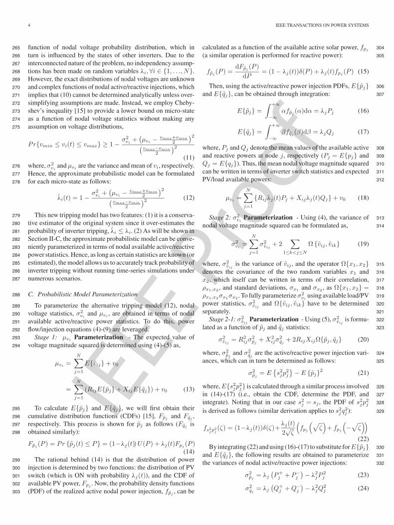
Fig. 2. Structure of the 240-node test system.

constraints:544

a0a0a0 + (B − IN )λλλ +

⎡

⎢⎢⎣

C1 • Λ...

CN • Λ

⎤

⎥⎥⎦− εεε+ ≤ 000 (50)

− a0a0a0 − (B − IN )λλλ −

⎡

⎢⎢⎣

C1 • Λ...

CN • Λ

⎤

⎥⎥⎦+ εεε− ≤ 000 (51)

∀i, j :

⎧⎪⎨

⎪⎩

Λ(i, i) + Λ(j, j)− 2Λ(i, j) ≥(λ(i)− λ(j)

)2

Λ(i, i) + Λ(j, j) + 2Λ(i, j) ≥(λ(i) + λ(j)

)2

(52)

where, Ci • Λ =∑N

n=1

∑Nm=1{Ci(n,m)Λ(n,m)}, IN is an545

N ×N identity matrix, and εεε+/εεε+ are positive/negative small-546

valued slack variables that are used for transforming equality547

constraints defined by the model into two equivalent inequal-548

ity constraints. The obtained inequalities (50)–(52) are convex549

constraints with respect to variables λλλ and Λ.550

IV. NUMERICAL EXPERIMENTS AND VALIDATION551

Numerical experiments have been performed to validate the552

proposed probabilistic tripping model. In this, we have used real553

feeder model of an Iowa distribution system from our utility554

partner as shown in Fig. 2. The network model in OpenDSS555

and detailed parameters are available online [35]. To perform556

simulations we have used real solar and load data with 1-second557

time resolution from [36]. Fig. 3 shows the PV outputs at558

different nodes in the system for one day. Fig. 4 demonstrates559

15-minute average nodal demand. The load/PV data have been560

randomly distributed across the three phases of the unbalanced561

grid at each node.562

To verify the performance of the proposed approximate statis-563

tical model, extensive time-series simulations were performed564

on the test system under various loading and solar generation565

scenarios over a course of day. Then, the real values of original566

micro-states, λi, were determined empirically over time win-567

dows of length T = 60 minutes. Intuitively, λi serves as the568

ground truth and roughly represents the portion of time that si569

Fig. 3. Nodal PV outputs in the test system.

Fig. 4. Average 15-minute nodal consumption in the test system.

is ON during each time window: 570

λi(T ) ≈∑T

t=1 si(t)

T(53)

Thus, we have two distinct time windows throughout numerical 571

studies: a 1-second time step is used to perform high-resolution 572

simulations, and a 1-hour time window is employed to obtain 573

tripping statistics and empirically verify the performance of 574

the proposed probabilistic model. Fig. 5a demonstrates the em- 575

pirical micro-states, λi, at different time intervals, which are 576

determined by applying (53) to simulation outcomes. Based 577

on the values of these micro-states, the empirical macro-state 578

value is calculated at all time intervals, which represents the 579

expected percentage of PV switches in ON state, i.e., Sp(T ) ≈ 580∑N

i=1 λi(T )N × 100. Fig. 5b compares the empirical macro-state 581

value and the lower bound value constructed using solutions of 582

(47). As can be seen, the solution from the probabilistic model 583

actually represents a lower bound to the empirical macro-state 584

obtained from simulations at all time windows, which corrob- 585

orates the performance of the method. This figure also shows 586

another lower bound obtained by simply using maximum PV 587

capacities and assuming zero nodal consumption. However, as 588

can be seen, this lower bound gives fixed over-conservative 589

outcomes that do not reflect the true conditions of the system and 590

have no correlation with the time-series PV/load data. Fig. 5c de- 591

picts the aggregate maximum available solar power (all switches 592

ON at all time), empirical aggregate realized solar power from 593

numerical simulations (53), and solar power corresponding to 594

solution of (47). As observed, the lower bound solution still 595

IEEE P

roof


Fig. 5. Comparing the empirical and statistical lower bound solutions.

holds and provides a conservative yet close estimation for the596

empirical achievable solar power outcome. Fig. 6 compares the597

empirical and model-based probabilities of inverter tripping in598

a heavy-loaded time interval. Unlike the previous case, these599

tripping probabilities are due to under-voltages. As can be600

observed, the model still provides a conservative lower bound601

on the probability of tripping. Note that the reason for higher602

levels of volatility in this figure is the shorter time window (15603

minutes) used for assessing the empirical probability of tripping.604

The gap between the empirical macro-state obtained from605

numerical experiments and the proposed lower bound is an606

implicit function of PV penetration. Sensitivity analysis was607

performed to quantify the relationship between this gap and PV608

penetration percentage, as shown in Fig. 7. Here, PV penetration609

is defined as the mean value of peak nodal solar power over peak610

nodal demand. The maximum, minimum, and mean values of611

the gap between the provided lower bound and the empirical612

Fig. 6. Model performance for a case of heavy-loaded system and 15-minuteempirical tripping probability assessment time window.

Fig. 7. Lower bound gap as a function of PV integration.

Fig. 8. Solar curtailment sensitivity to inverter control setpoints.

macro-state is measured at various levels of PV penetration. As 613

is observed in the figure, the optimistic value of the gap drops 614

and eventually reaches 5% as PV penetration increases, which 615

indicates that the lower bound approaches the true macro-state 616

value in grids with higher PV penetration. On the other hand, 617

the maximum value of the gap shows an increase after a certain 618

PV penetration level which points out to higher variations in 619

solutions obtained from the probabilistic model. 620

Fig. 8 shows the overall daily solar curtailment levels, both 621

empirical and the lower bound, as a function of changes in in- 622

verter control parameter. The inverters in the system are assumed 623

to be controlled in constant power factor (PF) mode. As the 624

reference PF setpoint increases and the system moves towards 625

unity PF the voltage fluctuations increase, which leads to higher 626

solar curtailment. This confirms previous observations in the 627

IEEE P

roof


Fig. 9. Solar curtailment countermeasure design verification.

literature [9]. Furthermore, our proposed probabilistic lower628

bound always slightly over-estimates the curtailment level, as629

expected correctly from the conservative estimator.630

Further tests were performed to corroborate the performance631

of countermeasure design strategy introduced in (48). Fig. 9a632

shows the outcome of the optimization problem (48), compared633

to a base case without any voltage regulation. As observed, v0634

is optimally decreased during solar-rich intervals to compensate635

for the increased voltage fluctuation levels. Fig. 9b compares the636

aggregate solar power injection values under the newly acquired637

v0 values and the base case without voltage control. As can be638

seen, the obtained countermeasure has assisted significantly in639

mitigating the overall solar power curtailments during critical640

time intervals.641

We have performed another numerical experiment to analyse642

and verify the behavior of our tripping model during an under-643

voltage case study in a temporary heavy loading scenario in a644

weak grid under two strategies (see Fig. 10): (1) No voltage regu-645

lation is applied (baseline), and (2) Voltage regulation is applied646

with the objective of minimizing the average squared voltage647

deviations across the whole system, subject to linearized power648

flow equations and the proposed statistical tripping model. As649

can be seen in Fig. 10a, under the baseline strategy (no voltage650

regulation) a portion of inverters (around 13%) have tripped651

due to under-voltage protection during later hours of the day.652

This has resulted in a loss of renewable power injection in the653

grid (Fig. 10b). However, by applying voltage regulation using654

the proposed tripping model we have been able to maintain the655

voltages much closer to their nominal values (see Fig. 10c) and656

prevent tripping events and loss of solar generation resources657

altogether. Note that Fig. 10c shows the average value of nodal658

Fig. 10. An under-voltage case study.

voltages across the whole system; thus, while most of the nodes 659

maintain healthy voltage levels (as they should), the excessive 660

loading on weak system lines under the baseline has resulted to 661

a temporary voltage drop below inverters’ protection activation 662

threshold, which has engaged their under-voltage protection 663

devices. This issue was mitigated using the deployed voltage 664

regulation strategy that leverages our proposed statistical trip- 665

ping model. 666

Fig. 11 demonstrates the average realized daily PV power 667

ratio as a function of average PV penetration. As can be seen, 668

the increasing penetration of solar has led to a regime shift after 669

a certain threshold, from an initial state, in which the system 670

shows almost no extensive tripping, to a new state, in which the 671

average probability of solar curtailment steadily increases and 672

extended tripping events can be expected. The existence of this 673

threshold attests to a stage transition in the extent of switching 674

events, which has been observed in other nonlinear systems 675

as well [26]. Above the PV integration threshold, which is 676

around 30% for the test system, massive solar curtailment can be 677

expected due to voltage fluctuations. It can be observed that the 678

proposed statistical lower bound accurately tracks the behavior 679

IEEE P

roof


Fig. 11. Regime shift (stage transition) analysis.

of the real system, and can be used to convey information on the680

whereabouts of the transition. The exact value of the regime shift681

threshold depends on many factors, including network topology682

and spatial-temporal distribution of loads/generators.683

V. CONCLUSION684

In this paper, a probabilistic model of interdependent solar685

inverter tripping is presented to assess the risk of solar power686

curtailments due to voltage fluctuations in distribution grids.687

This model is developed using only the statistical properties of688

available load/PV active/reactive power. Numerical results on a689

real distribution feeder using real data successfully validate the690

estimated conservative lower bounds on inverter micro-states.691

Furthermore, it is demonstrated that the proposed model can692

be used for identifying regime shifts in tripping events and693

designing countermeasures to minimize risk of solar power694

curtailment. As a future research direction, we will explore695

integrating the more dynamic functions of inverter control and696

protection, including ride-through capabilities, [17]–[20] into697

the probabilistic tripping model. For example, the proposed698

statistical lower bound, which is based on Chebyshev‘s inequal-699

ity, might become too conservative over short time windows if700

inverters’ disturbance ride-through capabilities are activated. A701

less conservative lower bound that incorporates all aspects of702

inverter behavior will enable operators to monitor the sequence703

and transitions of tripping events, and mitigate potential cascad-704

ing failure of resources.705

REFERENCES706

[1] R. Tonkoski, D. Turcotte, and T. H. M. El-Fouly, “Impact of high PV707penetration on voltage profiles in residential neighborhoods,” IEEE Trans.708Sustain. Energy, vol. 3, no. 3, pp. 518–527, Jul. 2012.709

[2] O. Gagrica, P. H. Nguyen, W. L. Kling, and T. Uhl, “Microinverter710curtailment strategy for increasing photovoltaic penetration in low-voltage711networks,” IEEE Trans. Sustain. Energy, vol. 6, no. 2, pp. 369–379,712Apr. 2015.713

[3] M. Hasheminamin, V. G. Agelidis, V. Salehi, R. Teodorescu, and B.714Hredzak, “Index-based assessment of voltage rise and reverse power flow715phenomena in a distribution feeder under high PV penetration,” IEEE J.716Photovolt., vol. 5, no. 4, pp. 1158–1168, Jul. 2015.717

[4] V. Ferreira, P. M. S. Carvalho, L. A. F. M. Ferreira, and M. D. Ilic, “Dis-718tributed energy resources integration challenges in low-voltage networks:719Voltage control limitations and risk of cascading,” IEEE Trans. Sustain.720Energy, vol. 4, no. 1, pp. 82–88, Jan. 2013.721

[5] P. M. S. Carvalho, L. A. Ferreira, J. C. Botas, M. D. Ilic, X. Miao, 722and K. D. Bachovchin, “Ultimate limits to the fully decentralized power 723inverter control in distribution grids,” in Proc. Power Syst. Comput. Conf., 724Jun. 2016, pp. 1–7. 725

[6] P. M. S. Carvalho, L. A. Ferreira, and J. J. E. Santana, “Single-phase 726generation headroom in low-voltage distribution networks under reduced 727circuit characterization,” IEEE Trans. Power Syst., vol. 30, no. 2, pp. 1006– 7281011, Mar. 2015. 729

[7] C. Popiel and P. D. H. Hines, “Understanding factors that influence the 730risk of a cascade of outages due to inverter disconnection,” in Proc. North 731Amer. Power Symp., 2019, pp. 1–6. 732

[8] A. Parchure, S. J. Tyler, M. A. Peskin, K. Rahimi, R. P. Broadwater, 733and M. Dilek, “Investigating PV generation induced voltage volatility for 734customers sharing a distribution service transformer,” IEEE Trans. Ind. 735Appl., vol. 53, no. 1, pp. 71–79, Jan. 2017. 736

[9] D. Cheng, B. A. Mather, R. Seguin, J. Hambrick, and R. P. Broadwater, 737“Photovoltaic (PV) impact assessment for very high penetration levels,” 738IEEE J. Photovolt., vol. 6, no. 1, pp. 295–300, Jan. 2016. 739

[10] P. Gupta, K. Rahimi, R. Broadwater, and M. Dilek, “Importance of detailed 740modeling of loads/PV systems connected to secondary of distribution 741transformers,” in Proc. North Amer. Power Symp., Sep. 2017, pp. 1–6. 742

[11] F. Ding and B. Mather, “On distributed PV hosting capacity estimation, 743sensitivity study, and improvement,” IEEE Trans. Sustain. Energy, vol. 8, 744no. 3, pp. 1010–1020, Jul. 2017. 745

[12] X. Xu, Z. Yan, M. Shahidehpour, H. Wang, and S. Chen, “Power system 746voltage stability evaluation considering renewable energy with correlated 747variabilities,” IEEE Trans. Power Syst., vol. 33, no. 3, pp. 3236–3245, 748May 2018. 749

[13] H. Jiang, Y. Zhang, J. J. Zhang, D. W. Gao, and E. Muljadi, 750“Synchrophasor-based auxiliary controller to enhance the voltage stability 751of a distribution system with high renewable energy penetration,” IEEE 752Trans. Smart Grid, vol. 6, no. 4, pp. 2107–2115, Jul. 2015. 753

[14] K. I. Jennett, C. D. Booth, F. Coffele, and A. J. Roscoe, “Investigation of 754the sympathetic tripping problem in power systems with large penetrations 755of distributed generation,” IET Gener. Transmiss. Distrib., vol. 9, no. 4, 756pp. 379–385, Dec. 2014. 757

[15] S. M. Ross, Introduction to Probability Models. New York, NY, USA: 758Academic, 2006. 759

[16] “WECC PV power plant dynamic modeling guide,” Western Electric- 760ity Coordinating Council, Tech. Rep., Apr. 2014. [Online]. Available: 761https://www.wecc.org/Reliability/WECC 762

[17] “NERC reliability guideline: Integrating inverter-based resources 763into weak power systems - Dec. 2017.” [Online]. Available: 764https://www.nerc.com/comm/PC_Reliability_Guidelines_DL/Item_4a._ 765Integrating%20_Inverter-Based_Resources_into_Low_Short_Circuit_ 766Strength_Systems_-_2017-11-08-FINAL.pdf 767

[18] “Australian Energy Market Operator (AEMO) Information & 768Support Hub: Multiple voltage disturbance ride-through capa- 769bility, justification of AEMO’s proposal - Mar. 2018.” [On- 770line]. Available: https://www.aemc.gov.au/sites/default/files/2018- 77103/AEMO%20report%20updated%20proposed%20multiple%20fault% 77220withstand%20obligation.pdf 773

[19] “Australian Energy Market Operator (AEMO) Information & Support 774Hub: Electricity rule change proposal, generator technical requirement 775- Aug. 2017.” [Online]. Available: https://www.aemo.com.au/- 776/media/Files/Electricity/NEM/Security_and_Reliability/Reports/2017/ 777AEMO-GTR-RCP-110817.pdf 778

[20] M. G. Dozein, P. Mancarella, T. K. Saha, and R. Yan, “System strength 779and weak grids: Fundamentals, challenges, and mitigation strategies,” in 780Proc. Australas. Universities Power Eng. Conf., 2018, pp. 1–7. 781

[21] N. Li, G. Qu, and M. Dahleh, “Real-time decentralized voltage control in 782distribution networks,” in Proc. 52nd Annu. IEEE Conf. Commun., Control, 783Comput. (Allerton), Oct. 2014, pp. 582–588. 784

[22] R. Singh, B. C. Pal, and R. A. Jabr, “Statistical representation of distri- 785bution system loads using Gaussian mixture model,” IEEE Trans. Power 786Syst., vol. 25, no. 1, pp. 29–37, Feb. 2010. 787

[23] D. T. Nguyen, “Modeling load uncertainty in distribution network moni- 788toring,” IEEE Trans. Power Syst., vol. 30, no. 5, pp. 2321–2328, Sep. 2015. 789

[24] L. Hatton, P. Charpentier, and E. Matzner-Lober, “Statistical estimation of 790the residential baseline,” IEEE Trans. Power Syst., vol. 31, no. 3, pp. 1752– 7911759, May 2016. 792

[25] H. L. van der Walt, R. C. Bansal, and R. Naidoo, “PV based distributed 793generation power system protection: A review,” Renewable Energy Focus, 794vol. 24, pp. 33–40, Mar. 2018. 795

[26] S. Thurner, R. Hanel, and P. Klimek, Introduction to the Theory of Complex 796Systems. London, U.K.: Oxford Univ. Press, 2018. 797

IEEE P

roof


[27] M. Mezard and J. Sakellariou, “Exact mean-field inference in asymmetric798kinetic Ising systems,” J. Statistical Mech.: Theory Exp., vol. 2011, no. 7,799Jul. 2011, Art. no. L07001.800

[28] A. Arif, Z. Wang, J. Wang, B. Mather, H. Bashualdo, and D. Zhao, “Load801modeling—A review,” IEEE Trans. Smart Grid, vol. 9, no. 6, pp. 5986–8025999, Nov. 2018.803

[29] J. O. Petinrin and M. Shaaban, “Impact of renewable generation on voltage804control in distribution systems,” Renewable Sustain. Energy Rev., vol. 65,805pp. 770–783, 2016.806

[30] D. Ranamuka, A. P. Agalgaonkar, and K. M. Muttaqi, “Online voltage807control in distribution systems with multiple voltage regulating devices,”808IEEE Trans. Sustain. Energy, vol. 5, no. 2, pp. 617–628, Apr. 2014.809

[31] T. T. Ku, C. H. Lin, C. S. Chen, and C. T. Hsu, “Coordination of trans-810former on-load tap changer and PV smart inverters for voltage control of811distribution feeders,” IEEE Trans. Ind. Appl., vol. 55, no. 1, pp. 256–264,812Feb. 2019.813

[32] W. K. K. Ma, “Semidefinite relaxation of quadratic optimization problems814and applications,” IEEE Signal Process. Mag., vol. 1053, no. 5888/10,815May 2010.816

[33] S. Kim and M. Kojima, “Second order cone programming relaxation817of nonconvex quadratic optimization problems,” Optim. Methods Softw.,818vol. 15, no. 3–4, pp. 201–224, Jan. 2001.819

[34] M. Kheirandishfard, F. Zohrizadeh, and R. Madani, “Convex relaxation820of bilinear matrix inequalities part i: Theoretical results,” in Proc. IEEE821Conf. Decis. Control, Dec. 2018, pp. 67–74.822

[35] F. Bu, Y. Yuan, Z. Wang, K. Dehghanpour, and A. Kimber, “A time-series823distribution test system based on real utility data,” 2019. [Online]. Avail-824able: https://arxiv.org/abs/1906.04078825

[36] C. Holcomb, “Pecan Street Inc.: A test-bed for NILM,” in Proc.826Int. Workshop Non-Intrusive Load Monit., 2012. [Online]. Available:827https://www.pecanstreet.org/828

Kaveh Dehghanpour (Member, IEEE) received the829B.Sc. and M.S. degrees in electrical and computer830engineering from the University of Tehran, Tehran,831Iran, in 2011 and 2013, respectively, and the Ph.D.832degree in electrical engineering from Montana State833University, Bozeman, MT, USA, in 2017. He is cur-834rently a Postdoctoral Research Associate with Iowa835State University, Ames, IA, USA. His research in-836terests include machine learning and data mining for837monitoring and control of smart grids, and market-838driven management of distributed energy resources.839

840

Yuxuan Yuan (Student Member, IEEE) received 841the B.S. degree in electrical and computer engi- 842neering in 2017 from Iowa State University, Ames, 843IA, USA, where he is currently working toward the 844Ph.D. degree. His research interests include distribu- 845tion system state estimation, synthetic networks, data 846analytics, and machine learning. 847

848

Fankun Bu (Student Member, IEEE) received the 849B.S. and M.S. degrees from North China Electric 850Power University, Baoding, China, in 2008 and 2013, 851respectively, and the Ph.D. degree from Iowa State 852University, Ames, IA, USA. From 2008 to 2010, he 853was a Commissioning Engineer for NARI Technol- 854ogy Co., Ltd., Nanjing, China. From 2013 to 2017, he 855was an Electrical Engineer for State Grid Corporation 856of China at Jiangsu, Nanjing, China. His research 857interests include distribution system modeling, smart 858meter data analytics, renewable energy integration, 859

and power system relaying. 860861

Zhaoyu Wang (Member, IEEE) received the B.S. 862and M.S. degrees in electrical engineering from 863Shanghai Jiaotong University, Shanghai, China, in 8642009 and 2012, respectively, and the M.S. and Ph.D. 865degrees in electrical and computer engineering from 866the Georgia Institute of Technology, Atlanta, GA, 867USA, in 2012 and 2015, respectively. He is currently 868the Harpole-Pentair Assistant Professor with Iowa 869State University, Ames, IA, USA. His research in- 870terests include power distribution systems and mi- 871crogrids, particularly on their data analytics and op- 872

timization. He is the Principal Investigator for a multitude of projects focused 873on these topics and funded by the National Science Foundation, the Department 874of Energy, National Laboratories, PSERC, and Iowa Energy Center. He is the 875Secretary of IEEE Power and Energy Society (PES) Award Subcommittee, a Co- 876Vice Chair of PES Distribution System Operation and Planning Subcommittee, 877and a Vice Chair of PES Task Force on Advances in Natural Disaster Mitigation 878Methods. He is an Editor for the IEEE TRANSACTIONS ON POWER SYSTEMS, 879IEEE TRANSACTIONS ON SMART GRID, IEEE PES LETTERS, and IEEE OPEN 880ACCESS JOURNAL OF POWER AND ENERGY, and an Associate Editor for IET 881Smart Grid. 882

883

ieee transactions on power systems 1 statistical …

Documents