ieee transactions on parallel and … · cost-aware big data processing across geo-distributed...

1045-9219 (c) 2016 IEEE. Personal use is permitted, but republication/redistribution requires IEEE permission. See http://www.ieee.org/publications_standards/publications/rights/index.html for more information.

This article has been accepted for publication in a future issue of this journal, but has not been fully edited. Content may change prior to final publication. Citation information: DOI 10.1109/TPDS.2017.2708120, IEEETransactions on Parallel and Distributed Systems

IEEE TRANSACTIONS ON PARALLEL AND DISTRIBUTED SYSTEMS, VOL. ×, NO. ×, 2016 1

Cost-Aware Big Data Processing acrossGeo-distributed Datacenters

Wenhua Xiao, Weidong Bao, Xiaomin Zhu, Member, IEEE , and Ling Liu, Fellow, IEEE

Abstract—With the globalization of service, organizations continuously produce large volumes of data that need to be analysed overgeo-dispersed locations. Traditionally central approach that moving all data to a single cluster is inefficient or infeasible due to thelimitations such as the scarcity of wide-area bandwidth and the low latency requirement of data processing. Processing big data acrossgeo-distributed datacenters continues to gain popularity in recent years. However, managing distributed MapReduce computationsacross geo-distributed datacenters poses a number of technical challenges: how to allocate data among a selection of geo-distributeddatacenters to reduce the communication cost, how to determine the VM (Virtual Machine) provisioning strategy that offers highperformance and low cost, and what criteria should be used to select a datacenter as the final reducer for big data analytics jobs. Inthis paper, these challenges is addressed by balancing bandwidth cost, storage cost, computing cost, migration cost, and latency cost,between the two MapReduce phases across datacenters. We formulate this complex cost optimization problem for data movement,resource provisioning and reducer selection into a joint stochastic integer nonlinear optimization problem by minimizing the five costfactors simultaneously. The Lyapunov framework is integrated into our study and an efficient online algorithm that is able to minimizethe long-term time-averaged operation cost is further designed. Theoretical analysis shows that our online algorithm can provide anear optimum solution with a provable gap and can guarantee that the data processing can be completed within pre-defined boundeddelays. Experiments on WorldCup98 web site trace validate the theoretical analysis results and demonstrate that our approach is closeto the offline-optimum performance and superior to some representative approaches.

Index Terms—Big Data Processing; Cloud Computing; Data Movement; Virtual Machine Scheduling; Online Algorithm.

F

1 INTRODUCTION

We are entering a big data era with more data generated andcollected in a geographically distributed manner in many areassuch as finance, medicine, social web, astronomy etc. With theincreasing explosion of distributed data, the huge treasures hiddenin it are waiting for us to explore for providing valuable insights.To illustrate, social web sites such as Facebook can uncoverusage patterns and hidden correlations by analyzing the website history records (e.g., click records, activity records et al.) todetect social hot event and facilitate its marketing decision (e.g.,advertisement recommendation), and the Square Kilometre Array(SKA) [1], an international project to build the world’s largesttelescope distributed over several countries, need to fusion thegeographically dispersed data for scientific applications. However,due to the properties such as large-scale volume, high complexityand dispersiveness of big data coupled with the scarcity of Wide-area bandwidth (e.g., trans-oceanic link ), it is inefficient and/orinfeasible to process the data with centralized solutions [2]. Thishas fueled strong companies from industry to deploy multi-datacenter cloud and hybrid cloud. These cloud technologies offera powerful and cost-effective solution to deal with increasinglyhigh velocity of big data generated from geo-distributed sources(e.g., Facebook, Google and Microsoft etc). For majority ofthe commmon organizations (e.g., SKA), it is economic to rentresource from public cloud, with considering the advantages of

Wenhua Xiao, Weidong Bao and Xiaomin Zhu are with the Science andTechnology on Information Systems Engineering Laboratory, National Uni-versity of Defense Technology, Changsha, Hunan, P. R. China, 410073. E-mail:{wenhuaxiao, wdbao, xmzhu}@nudt.edu.cnLing Liu is with the college of computing at Georgia Institute of Technology,266 Ferst Drive, Atlanta, GA 30332-0765, USA. E-mail:[email protected]

cloud computing such as flexibility and pay-as-you-go businessmodel.

MapReduce is a distributed programming model for process-ing large-scale dataset in parallel, which has shown its outstandingeffectiveness in many existing applications [3], [4], [5]. Sinceoriginal MapReduce model is not optimized for deployment acrossdatacenters [6], aggregating distributed data to a single datacenterfor centralized processing is a widely-used approach. However,waiting for such centralized aggregation suffers from significantlydelays due to the heterogenous and limited bandwidth of user-cloud link. Notice that the bandwidth of inter-datacenter linkis usually dedicated relatively high-bandwidth lines [7], movingthe data to multiple datacenters for map operation in paralleland then aggregating the intermediate data to a single datacenterfor reduce operation using inter-datacenter link has potential toreduce the latency. Furthermore, different kinds of cost (e.g.,incurred by moving data or renting VM) also can be optimizedconsidering the heterogeneity of the link speed, the dynamism ofthe data generation and the resource price. Therefore, distributingdata from multi-sources into multi-datacenters and processingthem using distributed MapReduce is an idea way to deal withthe large volume dispersed data. Hitherto, the most importantquestions to be solved include: 1) how to optimize the placementof large-scale datasets from various locations onto geo-distributeddatacenter cloud for processing and 2) how many resourcessuch as computing resources should be provisioned to guaranteeperformance and availability while minimizing the cost. The fluc-tuation and multiple sources of generated data combined with thedynamic utility-driven pricing model of cloud resource make it avery challenging problem. The inter-dependency between multiplestages of distributed computation, such as the interplay between




the Map phase and the Reduce phase of MapReduce programs,further escalates the complexity of the data movement, resourceprovisioning and final reduce selection problems in geo-distributeddatacenters.

In this paper, we address the problem of efficient schedulingwith the goal of high performance, high availability and costminimization by balancing five types of cost between the twoMapReduce phases across multiple geo-distributed datacenters:bandwidth cost, storage cost, computing cost, migration cost, andlatency cost.

Contributions: The major contributions of this work aresummarized as follows:

• We propose a framework that can systematically handlethe issues of data movement, resource provisioning as wellas reducer selection under the context of running MapRe-duce across multiple datacenters, and VMs of differenttypes and dynamic prices.

• We formulate the complex cost optimization problem as ajointed stochastic integer nonlinear optimization problemand solve it using Lyapunov optimization framework bytransforming the original problem into three independentsubproblems (data movement, resource provisioning andreduce selection) that can be solved with some simplesolutions. We design an efficient and distributed onlinealgorithm-MiniBDP that is able to minimize the long-termtime-averaged operation cost.

• We formally analyze the performance of MiniBDP interms of cost optimality and worst case delay. We showthat the algorithm approximates the optimal solution with-in provable bounds and guarantees that the data processingcan be completed within pre-defined delays.

• We conduct extensive experiments to evaluate the perfor-mance of our online algorithm with real world datasets.The experiments result demonstrate its effectiveness aswell its superiority in terms of cost, system stability anddecision-making time to existing representative approach-es (e.g., the combinations of data allocation strategies(proximity-aware, load balance-aware) and the resourceprovisioning strategies(e.g., stable strategy, heuristic strat-egy).

The remainder of this paper is organized as follows: Thenext section reviews related work in the literature; Section 3describes the system model and the problem formulation; Section4 presents the online algorithm for solving the problem; Theproposed algorithm is theoretically analyzed in section 5; Sectionpresents the experiments and performance analysis using real-world trace. Section 7 concludes the paper with a summary andfuture work.

2 RELATED WORK

Computation models. MapReduce [3] is a popular and efficientdistributed computing model that abstracts the data processing intotwo stages: Map and Reduce [6]. Extensions such as Twitter Storm[8] was proposed to handle real-time streaming data, Spark [4]was proposed as a solution that persistently keeps the distributedpartitions in memory to eliminate disk I/O latency. To supportdata processing with evolving property, several efforts [9], [10]have added iterative or incremental support for MapReduce tasks.Recently, to deal with the issue that both data and compute

Data

Source1

Data

Source2

M1 M2 M3

R1 R2 R3

Fig. 1: Architecture of Big Data Processing with MapReduceAcross Datacenters

resources are geo-distributed, the distributed MapReduce acrossdatacenters was proposed [11], [12], [13]. To improve the efficien-cy of large-scale data processing, Sfrent et al. [14] proposed anasymptotic scheduling mechanism for many computing tasks forbig data processing platforms. The common feature of these worksis considering a static scenario where the data are pre-stored in thecloud and the amount of data are fixed.

Wide-Area Big-Data (WABD) analytics. Work on WABD hasbeen a hot topic recently. Considering geo-dispersed data pro-cessing on clouds, Zhang et al. [7] proposed an online algorithmto migrate dynamically generated data from various locationsto the clouds and studied how to minimize the bandwidth costof transferring data for delay-tolerant processing with multipleInternet Service Providers (ISPs) [15]. Zhang et al. [16] studiedhow to efficiently schedule and perform analysis over data thatis geographically distributed across multiple datacenters and de-signed system-level optimizations including job localization, dataplacement and data pre-fetching for improving performance ofHadoop service provisioning in a geo-distributed cloud. Targetingat query analytics over geo-distributed datacenters, studies focuson different goals (e.g., either reducing bandwidth cost [2], [17],[18] or execution response time [19]). Geode [2] is proposed tosolve the problem of querying wide-area distributed data with goalof reducing bandwidth cost, but it makes no attempt to minimizeexecution latency and does not support general computations taskthat go beyond SQL query under MapReduce framework. WANa-lytics [17] is designed for arbitrary computation with DAGs of taskand proposed a heuristic algorithm to optimize tasks execution aswell as an intermediate data caching strategy to reduce bandwidthcost. PIXIDA [18] is proposed to minimize the traffic incurredfrom data movement across resource constrained links. In contrastto MiniBDP, it formulates the traffic minimization optimizationinto a graph partitioning problem. Iridium [19] is the closest worksince it also optimizes the data and task placement to achieve thegoal of minimizing the response time of query analysis acrossgeo-distributed sites. However, its approach is rather differentfrom MiniBDP since it needs to estimate the query arrivals andignores the CPU and storage cost. In addition, MiniBDP showsdelay bounds while Iridium does not.

Management of multiple datacenters . Managing multiple ge-ographically distributed datacenters has attracted companies suchas Facebook, Google, HP and Cisco. To support geo-distributed




hadoop data storage, Facebook developed a project Prism [20] byadding a logical abstraction layer to Hadoop cluster. Focusing onfault tolerance and load balancing, Google deployed its databasesystem Spanner [21] in a distributed manner, which is able toautomatically migrating data across datacenters. HP [22] andCisco [23] have also made efforts to manage their geo-distributeddatacenters by optimizing the inter-datacenters network on thelayer of data link. However, current practical methods are limitedby their transport dependency, complexity and lack of resilience.Further, these methods mainly focus on providing better servicequality for increasingly global user demands but not on datacomputations.

Recently, Lyapunov optimization technique was [24] appliedto cloud computing contex to deal with job admission and resourceallocation problem [25], [26]. Yao et al. [27] extends it from thesingle time scale to two-time-scale for achieving electricity costreduction in geographically distributed datacenters. Besides, thisapproach is used for resource management in cloud-based videoservice [28], [29]. In this paper, we apply this technique to addressthe issue of data moving and resource provisioning for big dataprocessing in cloud with geo-distributed MapReduce.

To summarize, differs to aforementioned studies, our goalis to minimize overall cost when processing geo-dispersed bigdata across multiple datacenters, by balancing computation cost,bandwidth cost, storage cost, migration cost and latency cost,not only one or part of them. Further, we incorporate dynamicresource provisioning into the framework and make decision onthe data movement, resource provisioning and reducer selectionsimultaneously at a long run. In addition, we consider the problemon the granularity of Map and Reduce as well as the data flowbetween the two phases that support incremental style acrossdistributed datacenters .

3 MODELING AND FORMULATION

In this section, we first introduce the preliminary knowledge onMapReduce and the execution path of data over geo-distributeddatacenters, and then we present the system model.

3.1 PreliminariesIn MapReduce model, Mapper process the input datasets and output a set of < key, value > intermediate pairs at Map phase, whileReducer receive all the intermediate data from mappers and mergethe values according to a specific key to produce smaller sets ofvalues at Reduce phase. Both of them can be deployed in differentnodes.

Under the environment of distributed datacenters, the execu-tion path of geo-distributed data is of particular importance. Asconcluded by Chamikara et.al. [12], there are three executionpaths for data processing with MapReduce across datacenters:COPY, MULTI and GEO. COPY is a strategy that copies allthe sub-datasets into a single datacenter before handing themwith MapReduce. However, it is inefficient when the outputdata generated by MapReduce is much smaller than the inputs.MULTI is a strategy that executes MapReduce job separately oneach sub-dataset and then aggregates the individual results. Thedrawback of this strategy lies in that the expected outcome isyielded only if the order of the MapReduce jobs does not havean impact on the final result. GEO is a strategy that executesthe Map operation in different datacenters and then copy theintermediate data to a single datacenter for Reduce operation. This

is suitable for those applications where the jobs are correlated inthe Reduce phase, e.g., determining the median size of the pagesin a Web cache, or those applications where the intermediate datais smaller than the input. As reported in [13], by measuring theHadoop traces of about 16000 jobs from Facebook, there are about70% of jobs whose input data is larger than the correspondingintermediate data. Therefore, GEO conducts the map operation ineach datacenter and then aggregates the intermediate data into asingle datacenter will reduce cross-region bandwidth cost. Basedon above consideration, we consider the GEO execution path inproblem modelling.

3.2 System Model

Without loss of generality, we consider such a system scenariowhere a DSP (Data Service Provider) manages multiple datasources and transfers all the data into cloud for processing usingMapReduce. The DSP may either deploy its private datacenters(e.g., Google deploys tens of datacenters over the world) or rentthe resource from public clouds (e.g., SKA may rent the resourcefrom public cloud such as Amazon EC2). Specially, for the DSPthat have its private cloud, datasources overlaps datacenters sincegenerated data are collected and stored in its own datacenters.System architecture is presented in Fig. 1: Data sources from mul-tiple geographical data locations continuously produce massivedata. Data analysis applications are deployed in the cloud andthe data sources is connected to datacenters located in multipleplaces. In this model, data are moved to the datacenters once theyare generated and are processed in a incremental style in whichonly the newly arrived data are computed and the intermediatedata from past can be reused. Specifically, both mappers andreducers are running on every datacenter. As the GEO executionpath mentioned above is considered in this paper, there are twocorresponding phases for the data moving procedure. At the firstphase, data can be moved to any datacenter for Map operation. Atthe second phase, the intermediate data of Mappers must be movedinto a single datacenter with consideration of data correlations. Asshown in Fig. 1, the bold line is an example of execution path,which shows that the raw data from data source 1 and data source2 are moved to multiple datacenters for Map operation and thenthe output data of Mappers are aggregated into the Reducer indatacenter 1 for Reduce operation.

Formally, let D be the set of geographically distributed data-centers with size of D = |D| (indexed by d(1 ≤ d ≤ D) ) and Kbe the set of VM types with size K = |K|, each of which has aspecific capacity vk with configurations such as CPU and memory.All types of VMs can be provisioned in each datacenter. Data aredynamically and continuous generated from R = |R| differentdatasource locations (indexed by r, 1 ≤ r ≤ R), denoted as aset R. Data from any location can be moved to any datacenterfor Map operation and then aggregate the intermediate data intoa single datacenter. To be realistic, we assume that the bandwidthBrd from data location r to datacenter d is limited. Also notethat inter-datacenter links (e.g., trans-oceanic links) are expensiveto lay down, so the costs of using these links are considered asa first-order entity when migrating the intermediate data amongdatacenters. In addition, the data generation in each location isindependent and the prices of the resource (e.g., VM) in eachdatacenter are varied in both spatial and temporal domain.

The system runs according to time slots, which is denotedby t = 0, 1, ..., T . In each time slot, the DSP needs to make




TABLE 1: IMPORTANT NOTATIONS

D set of datacenters (DC)R set of data locationsK set of VM types

ar(t) amount of the data generated from datasource (DS) r at tAr

max max amount of data generated from DS r

λdr(t) amount of the data allocated to d from DS r at t

Nk,maxd max number of VMs of type-k in DC d

mkd(t) number of type-k VM provisioned for Map in DC d at t

nkd(t) number of type-k VM provisioned for Reduce in DC d at t

pkd(t) price of type-k VM in DC d at tsd price of storage in datacenter dbdr price of bandwidth between DS r and DC d

Udr uplink bandwidth between DS r and DC d

Ldr the latency between DS r and DC d

vk data processing rate of type-k VMϵd preset constant for controlling queueing delay in Md(t)σd preset constant for controlling queueing delay in Rd(t)l max delay of data process

Md(t) unprocessed data at Map phase in DC d at tRd(t) unprocessed data at Reduce phase in DC d at tYd(t) virtual queue associate with Md(t) to guarantee its delayZd(t) virtual queue associate with Rd(t) to guarantee its delay

the decision about moving how much data from data location rto datacenter d, renting how many resources to support its dataprocessing from each datacenter, and selecting which datacenterfor Reduce operation. Our goal therefore is to minimize the overallcost of big data analysis in clouds while guaranteeing the delayin the long run. For ease of reference, important notations aresummarized in Table 1.

3.3 Problem FormulationIn this subsection, based on the system model aforementioned, weformulate the problem mathematically as follows.

Decision variables. The three decisions to be made are:(1) Data allocation variable: λd

r(t), denotes the amount ofthe data allocated to d from data location r at t, which meansthat the data generated from each location can be moved to anydatacenter for analysis. Let ar(t) , Ar

max, Udr be the amount of

data generated from the r-th region at time slot t, the max volumeof data generated in location r and the upload capacity betweenregion r and datacenter d, respectively. Hence, we have:

ar(t) ≤ Armax, ∀r ∈ R, t ∈ [1, T ], (1)

ar(t) =∑d∈D

λdr(t), ∀r ∈ R, t ∈ [1, T ], (2)

0 ≤ λdr(t) ≤ Ud

r , ∀r ∈ R, d ∈ D, t ∈ [1, T ], (3)

where Eq.(2) ensures that the sum of data allocated to eachdatacenter at one time slot is equal to the total amount datagenerated at that time slot. Eq.(3) ensures that the total amountof data uploaded via link < r, d > should not exceed theupload capacity of link < r, d >. The variable set is denotedas λ(t) = {λd

r(t), ∀r ∈ R, ∀d ∈ D}.(2) VM provisioning variable: mk

d(t), nkd(t), ∀d ∈ D, ∀k ∈

K, denote the number of type-k VM rented from datacenter dat time slot t for Map and Reduce operation, respectively. Theycan be scaled up and down over time slots. Since the computationresource in a datacenter is limited, we let Nk,max

d be the maxnumber of type-k VM in datacenter d. Therefore, we have:

0 ≤ nkd(t) +mk

d(t) ≤ Nk,maxd , ∀d, ∀k, t ∈ [1, T ], (4)

which means that the amount of resource employed by Map andReduce operation cannot surpass the available resources in a spe-cific datacenter. We denote m(t) = {mk

d(t),∀d ∈ D,∀k ∈ K}.n(t) is defined similarly.

(3) Reducer selection variable: xd(t),∀d ∈ D. Since all theintermediate data from mappers will be aggregated into only onedatacenter for Reduce operation at time slot t, xd(t) needs to bedefined as a binary variable. It indicates whether datacenter d isthe target datacenter to execute Reduce operation at time slot t(xd(t) = 1) or not (xd(t) = 0). Formally, we have:∑

d∈Dxd(t) = 1, xd(t) ∈ {0, 1},∀t ∈ [1, T ], (5)

where∑d∈D

xd(t) = 1 ensures that there is only one datacen-

ter running Reducer at time slot t. We difined set x(t) ={xd(t),∀d ∈ D}.

Cost. The goal of the DSP is to minimize the overall cost in-curred in the system by optimizing the amount of data allocated toeach datacenter, the number of resources needed, and the suitabledatacenter for Reduce operation. Specifically, the following costcomponents are considered in this paper: bandwidth cost, storagecost, latency cost, computing cost and migration cost.

(1) Bandwidth cost, storage cost and the latency cost. Usually,the bandwidth price is varied over different VPN links becausethey often belong to different Internet service providers. Let bdr bethe price of transferring 1 GB data between data location r ∈ Rand datacenter d ∈ D, then the bandwidth cost of moving datainto cloud at t is:

∑d∈D

∑r∈R

λdr(t) · bdr . For storage cost, which is

an important factor to be considered in choosing the datacenter fordata analysis due to large amount of data for big data application.Let sd, Wd(t) represent the price of data storing and the amountof unprocessed data in datacenter d ∈ D respectively , thenthe storage cost at t is:

∑d∈D

∑r∈R

λdr(t) · sd +

∑d∈D

Wd(t) · sd.

In particular, it can be obtained that Wd(t) = Md(t) + Rd(t)from (17) and (19). The latency incurred by uploading data tothe datacenters is also an important performance measure, whichis to be minimized in the data moving process. Let Ld

r denotethe latency between the data location r ∈ R and the datacenterd ∈ D. These delays are mainly determined by the respectivegeographic distance and bandwidth of links. As suggested in [7],we convert the latency into monetary cost. Therefore, we candefine the latency cost as:

∑d∈D

∑r∈R

α · λdr(t) · Ld

r , where α is a

weight converting latency into a monetary cost. Therefore, thetotal cost of this part can be defined as:

Csbl(λ(t)) =∑d∈D

∑r∈R

λdr(t) · (sd + bdr + αLd

r)+∑d∈D

Wd(t)·sd.

(6)(2) Computing cost. Due to the variance of VM price over time

slots, the number of the VMs rented from datacenter has importantimpact on the overall cost of the system as well as QoS of the bigdata application. Let pkd(t) be the price of type-k VM in datacenterd at time slot t, which is diverse in both spatial and time space.Then the computing cost can be calculated as follows,

Cp (m(t),n(t))∆=

∑d∈D

∑k∈K

{mk

d(t) + nkd(t)

}· pkd(t). (7)

(3) Migration cost. In many applications, analyzing data notonly uses the data at current time but also needs the historical




data (e.g., incremental analytics re-use the previous computationresults rather than recompute them when new data arrives [9]).Therefore, the intermediate data including the historical onesgenerated by Map operations in other geo-distributed datacenterswill be transferred to the selected reducer, incurring a migrationcost. Without lost of generality, assuming the historical data fromµ previous time slots will be reused, we denote the amountof historical data to be transferred from datacenter i at t is

hi(t) =t−1∑

τ=t−µβτfi(τ), where fi(τ) represents the amount of

intermediate data generated in datacenter i at time τ . fi(τ) canbe estimated using the data processed at Map phase at time τsince there is a ratio (e.g., γ) between the raw data size and theintermediate data size for a specific application [30]. βτ ∈ [0, 1]indicates the ratio of historical data to be transferred. In particular,it satisfies βa < βb if a < b, which means the importance ofthe historical data declines as time goes by. The weight can bedetermined by the specific application. Furthermore, we denoteΦid(·) as a non-decreasing migration cost function (includingbandwidth cost and latency cost) for moving data from datacenteri to datacenter d, which can be defined based on the bandwidthprices and the geographic distances among datacenters. Also, itsatisfies Φid(·) = 0 when i = d because it is unnecessary totransfer data within the same datacenter. Hence, the total migrationcost incurred in the system at time slot t is:

Cmgr(m(t),x(t))∆=

∑d∈D

{xd(t)

∑i∈D

Φid(hi(t))

}. (8)

Based on above cost formulations, the overall cost incurred inthe system at time slot t can be calculated as:

C(m(t),n(t), λ(t),x(t)) = Cp(m(t),n(t)) + Csbl(λ(t))+Cmgr(m(t),x(t))

.

(9)Objective. The problem of minimizing the time-average cost

of data moving and processing within a long-term period [0, T ]can be formulated as:

P1. min : C (10)

s.t. : 0 ≤ λdr(t) ≤ Ud

r , ∀r,∀d, t ∈ [1, T ]; (11)

ar(t) =∑d∈D

λdr(t),∀r, t ∈ [1, T ]; (12)

0 ≤ nkd(t) +mk

d(t) ≤ Nk,maxd , ∀d, ∀k, t ∈ [1, T ]; (13)

mkd(t) ∈ Z+ ∪ 0, nk

d(t) ∈ Z+ ∪ 0, ∀d,∀k, t ∈ [1, T ];(14)∑

d∈Dxd(t) = 1, xd(t) ∈ {0, 1},∀t ∈ [1, T ]; (15)

λd ≤ md, F d ≤ nd, ∀d; (16)

where C∆= lim

T→∞1T

T−1∑t=1

C(m(t),n(t), λ(t),x(t)). λd is the

time-averaged data size allocated to datacenter d and md is time-averaged VM resource provisioned for Map phase at datdacenterd. F d represents the average intermediate data size input toReduce phase and nd is time-averaged VM resource provisionedfor Reduce phase at datdacenter d. Thus, the constraint (16)guarantees the stability of Map workload queue Md and Reduce

workload queue Rd, by ensuring that the arrival data rate is nohigher than the average process rate.

As the data generation is stochastic, x is an integer constrainedvariable and hi(t) is a nonlinear function, it can be easily verifiedthat the problem is a constrained stochastic integer nonlinearoptimization problem and our objective is to minimize the long-term average cost by optimizing the amount of data allocated toeach datacenter, the number of VMs rented from the datacentersas well as selecting the optimal reducer. However, it is ofteninfeasible to solve the problem efficiently in a centralized solutionwhen T is large. To deal with this complex problem, we employa recent developed optimization technique-Lyapnov optimization[31] as shown in the section 4.

4 ONLINE ALGORITHM DESIGN

An outstanding feature of Lyapunov optimization is that it does notneed future information about workload. By greedily minimizingthe drift-plus-penalty at each time slot, it can solve the long-termoptimization problem efficiently with a solution that can be provedto arbitrarily close to the optimum. Next, we first transform theproblem P1 to an optimization problem of minimizing the Lya-punov drift-plus-penalty term and then design the correspondingonline algorithm.

4.1 Problem TransformationQueues Design. As the incremental data processing style isconsidered in the paper, we model the data processing evolutionas a queue model. In each datacenter, to describe the two dataprocessing procedures (Map and Reduce) running in the system,we design the corresponding queues as follows.

(1) For the Map phase, let Md(t) be the amount of unpro-cessed data in Map queue in datacenter d at time slot t. The queueis initialized as Md(0) = 0, and then the update of the queueMd(t) can be described as follows:

Md(t+ 1) = max[Md(t)−∑k∈K

mkd(t) · vk, 0] +

∑r∈R

λdr(t).

(17)The above queue evolution implies that the amount of processeddata and newly-arrived data at Map phase are

∑k∈K

mkd(t) · vk and∑

r∈Rλdr(t), respectively.

To guarantee that the worst-case queuing delay in queueMd(t) , ∀d ∈ D, is bounded by the max Map workload delaylm, we design a related virtual queue Yd(t) according to the ϵ-persistent service technique for delay bounding in [32]. Similarly,the backlog of virtual queue Yd(t) is initialized as Yd(0) = 0,then it is updated as follows:

Yd(t+ 1) = max[Yd(t) + 1Md(t)>0(ϵd −∑k∈K

mkd(t) · vk)

−1Md(t)=0

∑k∈K

Nk,maxd · vk, 0],

(18)where the indicator function 1Md(t)>0 equals to 1 when Md(t) >0, and 0 otherwise. Similarly, 1Md(t)=0 equals to 1 when Md(t) =0, and 0 otherwise. ϵd is a preset constant that can be used tocontrol the bound of delay for Map queue. It can be proved thatwe are able to guarantee all data being processed with delays atmost lm time slots if the the length of Md(t) and Yd(t) overtime slots can be guaranteed. It is also proved that l can be set




as lm = [(Mmaxd + Y max

d )/ϵd], where Mmaxd and Y max

d are thebound of queues Md(t) and Yd(t) respectively. Details can beseen in Theorem 5.3.

(2) For the Reduce phase, similar to the Map phase, thecorresponding queue in datacenter d is denoted as Rd(t) withRd(0) = 0, and the updating of this queue can be calculated asfollows.

Rd(t+1) = max[Rd(t)−∑k∈K

nkd(t)vk, 0]+xd(t)·Fd(t), (19)

where Fd(t)=t−1∑

τ=t−µ(βτ

∑i∈D

fi(τ)) is the amount of intermedi-

ate data from other datacenters, including the historical data ofpast µ time slots. From the above equations, we can know that itadmit only part of the data generated within the same time slotis processed. So do moving its intermediate data to a reducer. Inreality, the system will wait for all the intermediate data to producethe final result.

Accordingly, its virtual queue can be defined as:

Zd(t+ 1) = max[Zd(t) + 1Rd(t)>0(σd −∑k∈K

nkd(t) · vk)

−1Rd(t)=0

∑k∈K

Nk,maxd · vk, 0].

(20)In theory, the worst case delay of queue Rd(t) can also be

guaranteed as shown in Theorem 5.3.Problem Transformation. Let M(t) = [Md(t)], Y(t) =

[Yd(t)], R(t) = [Rd(t)] and Z(t) = [Zd(t)], ∀d ∈ D denotethe matrix of Map queues and Reduce queues respectively. Then,to measure the congestion of data processing procedure, we useΘ(t) = [M(t);Y(t);R(t);Z(t)] to denote the combined matrixof Map queues and Reduce queues. Thus, the Lyapunov functionscan be defined as follows:

L(Θ(t)) =1

2

∑d∈D

{Md(t)2+ Yd(t)

2+Rd(t)

2+ Zd(t)

2},

(21)where L(Θ(t)) measures the queue backlogs in the system.Furthermore, to keep the stability of above queues by persistentlypushing the Lyapunov function to a low congestion state, the one-slot Lyapunov drift is introduced as:

∆(Θ(t)) = E{L(Θ(t+ 1))− L(Θ(t))|Θ(t)}. (22)

According to the Lyapunov optimization framework, the drift-plus-penalty, which balances the queue stability and system cost,can be obtained by adding the the cost incurred by the system tothe above Lyapunov drift, namely,

∆(Θ(t)) + V · E{C(m(t),n(t), λ(t),x(t))|Θ(t)}, (23)

where V is a non-negative weight that affects the balance betweenthe cost optimization and drift minimization. Intuitively, a larger Vwill causes a smaller cost, and vice versa. Therefore, the problemP1 can be transformed into problem P2 as following:

P2. min : (23) (24)

s.t. : (11)(12)(13)(14)(15). (25)

To solve problem P2, rather than directly minimizing the drift-plus-penalty expression (23), we seek to minimize the upper boundfor it, without undermining the optimality and performance ofthe algorithm according to [31]. The key point of the problem

is therefore to find an upper bound on the expression(23). It canbe proved that, under any decision strategy, the expression (23)satisfies:

∆(Θ(t)) + V · E{C(m(t),n(t), λ(t),x(t))|Θ(t)}≤ B

+E{ ∑

d∈D

∑k∈K

mkd(t) ·

(V pkd(t)−Md(t)vk − Yd(t)vk

)|Θ(t)

}+E

{ ∑d∈D

∑k∈K

nkd(t) ·

(V pkd(t)−Rd(t)vk − Zd(t)vk

)|Θ(t)

}+E

{ ∑d∈D

∑r∈R

λrd(t) ·

(V sd + V bdr + V αLd

r +Md(t))|Θ(t)

}+E

{ ∑d∈D

xd(t)

{V

∑i∈D

Φid(hi(t))+Rd

∑i∈D

hi(t)

}|Θ(t)

},

(26)where B = 2

∑d∈D

(∑k∈K

Nk,maxd vk)

2+ 1

2

∑d∈D

∑r∈R

λmaxr +

12

∑d∈D

((ϵd)2+ (σd)

2) + 1

2D(µβmax

∑d∈D

∑k∈K

Nk,maxd vk)

2. De-

tailed proof please refer to [31].

4.2 Online Control Algorithm DesignFortunately, by investigating the R.H.S (Right Hand Side) of (26),we can equivalently decouple the problem into three subproblems:1) data allocation, 2) resource provisioning and (3) reducer selec-tion. The details of the solution for the above three subproblemsare given as follows.

1) Data Allocation: On the R.H.S of (26), a carefully obser-vation on the relationship among different variables reveals thatthe data allocation problem can be written as follows:

E{∑d∈D

∑r∈R

λdr(t) ·(V sd+V bdr+V αLd

r+Md(t))|Θ(t)}. (27)

Furthermore, since the data generated at each datasource areindependent, the centralized optimization can be implementedindependently and distributedly at each datasource. Consideringthe data allocation in datasource r at time t, we should solve thefollowing problem.

min∑d∈D

λdr(t)[V sd + V bdr + V αLd

r +Md(t)]

s.t.(11)(12). (28)

In fact, problem (28) can be regarded as a generalized min-weight problem in which the amount of data from datasource rmoved to datacenter d (λd

r(t)) is weighted by the queue backlogMd(t) , bandwidth price bd, storage price sd and the latencycost L(r, d). Intuitively, the data inclines to be allocated to thedatacenter with the minimal value of weight [V sd + V bdr +V αLd

r+Md(t)]. Note the allocation variable λdr(t) is constrained

by the uplink capacity (i.e., 0 ≤ λdr(t) ≤ Ud

r ), we can allocate thedata to the datacenters within their uplink capacities accordingto their weight order. The detailed algorithm for solving thisproblem can be seen in Algorithm 1. Obviously, the complexity ofalgorithm 1 is with O(D × R), thus the averaged complexity ofeach element is with O(1). Obviously, the strategy exhibits thatall the left data can be allocated if the data to be moved (i.e.,aleft) is less than the corresponding uplink capacity. Otherwise,the amount of data equals to the uplink capacity (i.e.,Ud

r ) willbe allocated. Repeating the procedures above, all the data can beallocated until there is no left data.




Algorithm 1: The Algorithm of Solving λdr(t)

1 Input: α, V, Ldr ,Md(t), ar(t), sd, bdr , Ud

r (∀d ∈ D,∀r ∈ R)2 Output: λd

r(t)3 foreach r ∈ R do4 Sort Qr with ascending order where

Qdr = V sd + V bdr + V αLd

r +Md(t) ;5 Initialize aleft = ar(t);6 while Qr ̸= ∅ ∩ aleft > 0 do7 d = head(Qr);8 if Ud

r ≥ aleft then9 λd

r(t) = aleft;

10 else11 λd

r(t) = Udr ;

12 aleft = aleft − λdr(t);

2) Resource Provisioning: The part related to variable mkd(t)

and nkd(t) in the R.H.S of (26) can be regarded as resource

provisioning problem if we remove the constant term. Therefore,the optimal VM provisioning strategy can be obtained by solvingthe following problem:

minE{ ∑

d∈D

∑k∈K

mkd(t)

(V pkd(t)−Md(t)vk − Yd(t)vk

)|Θ(t)

}+E

{ ∑d∈D

∑k∈K

nkd(t)


)|Θ(t)

}s.t.(13)(14)

.

(29)As the resource provisionings in each datacenter are inde-

pendent, similar to data allocation, problem (29) also can besolved independently and distributedly within each datacenter.Considering the resource problem within datacenter d, we canrewrite it as (30).

minE{ ∑

k∈Kmk

d(t)(V pkd(t)−Md(t)vk − Yd(t)vk

)|Θ(t)

}+E

{ ∑k∈K

nkd(t)


)|Θ(t)

}s.t.(13)(14)

.

(30)Using the basic knowledge of linear programming, the so-

lution to the above linear problem can be derived as shown inEq.(31)(refer to next page), which indicates that a type-k VM ispreferred to be rented in t when its price pkd(t) is small, and theVM whose capacity, vk, is large is more likely to be rented too.

3) Reducer Selection: The part related to variable xd(t) inthe R.H.S of (26) is therefore considered as the reducer selectionproblem. It can be written as follows.

minE{∑d∈D

xd(t){V∑i∈D

Φid(hi(t))+Rd

∑i∈D

hi(t)}|Θ(t)}

s.t.(15).

(32)

Note that hi(t) =t−1∑

τ=t−µβτfi(τ) is known since fi(τ), τ ∈

[t−µ, t−1] is known at time slot t, it also becomes a min-weightproblem. Hence, it can be easily derived that:

xd(t) =

{1, d =d∗

0, else, (33)

Algorithm 2: Procedures of the Algorithm MiniBDP1 Input:2 Md(t), Yd(t), Rd(t), Zd(t), ar(t),vk, sd, b

dr , L

dr , µ, α, β, γ

Nk,maxd , Ar

max, pkd(t), V, α (∀d ∈ D, ∀r ∈ R, ∀k ∈ K)

3 Output:4 mk

d(t), nkd(t), λ

dr(t), xd(t) (∀d ∈ D,∀r ∈ R, ∀k ∈ K)

5 Resource provisioning:6 foreach datacenter d ∈ D do7 Get the VM provisioning strategies for Map (mk

d(t)) andReduce (nk

d(t)) by solving the problem (29) using (31);8 Data Allocation:9 foreach r ∈ R do

10 Get the data allocation strategy λdr(t) by solving the

problem (28) using algorithm 1;

11 Reducer Selection:12 Select the reducer to which aggregates the intermediate data

from Map phase by using (33) (i.e., xd(t) is obtained).13 Update the queues Md(t), Yd(t), Rd(t), Zd(t) according to

queue dynamic equation (17),(18),(19) and (20) respectively.

where d∗ = argmind{V∑i∈D

Φid(hi(t))+Rd

∑i∈D

hi(t)}.

So far, the three complex problems of data allocation, resourceprovisioning and reducer selection at time slot t have been solvedindependently and efficiently. The simple strategies facilitate theonline deployment of the algorithm in the real-world systems. Em-ploying the queue updating manner (17),(18),(19) and (20) alongtime slots, we can design an online algorithm called MiniBDP forsolving the problems in the long run. The details of the onlinealgorithm are presented in Algorithm 2.

5 PERFORMANCE ANALYSIS

Next, to show its superiority, the performance of the Algorithm ??in terms of cost optimality, queueing delay bound, and the worstdelay of data processing is theoretically analyzed.

Theorem 5.1. (Cost Optimality) Suppose the data generation ratear(t), ∀r ∈ R is identical an independently distributed overtime slots, for any control parameter V > 0, the algorithmcan achieve a time average cost related with the optimal oneas follows.

lim supT→∞

1

T·T−1∑t=0

E{C(t)} ≤ C∗ +B

V, (34)

where C∗ is the infimum of the time average cost when choos-ing the optimal control action, representing the theoreticallyoptimal solution, B is the same as defined in (26).

Proof: Please see the Appendix A in the supplemental file.This theorem exhibits that the gap between the time average

cost obtained by the algorithm proposed in this paper and theoptimal cost obtained offline is with O(1/V ). In particular, bychoosing the control variable V , the time-average cost C isarbitrarily close to the optimal cost C∗.

Theorem 5.2. (Queues Bound) Assume ϵd satisfies ϵd + σd <∑k∈K

Nk,maxd vk. Let Mmax

d , Y maxd , Rmax

d and Zmaxd be the

upper bound of queue Md(t), Yd(t), Rd(t) and Zd(t) respec-tively, we have:

Y maxd = Zmax

d = 2V pmax

d

vmin+ ϵd + σd, (35)




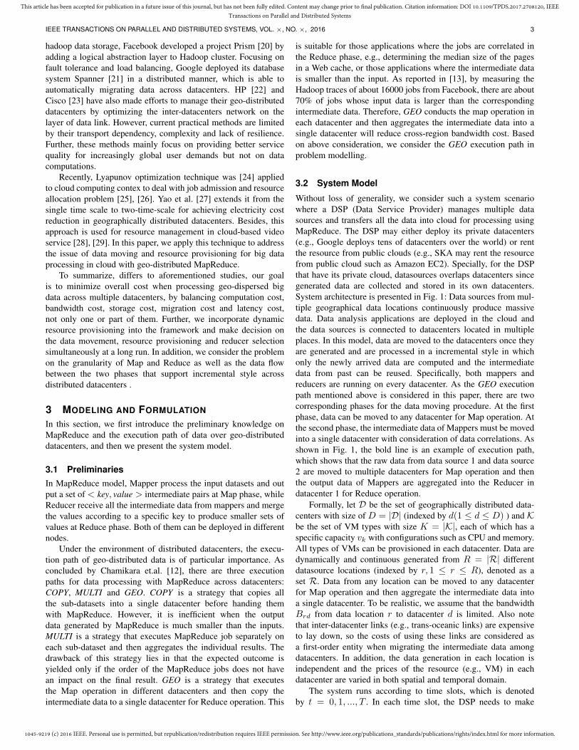
(mk

d(t), nkd(t)

)=

(0, 0) , ifMd(t) + Yd(t) ≤

V pkd(t)vk

∩Rd(t) + Zd(t) ≤V pk

d(t)vk(

Nk,maxd , 0

), ifRd(t) + Zd(t) ≤ Md(t) + Yd(t) ∩Md(t) + Yd(t) ≥

V pkd(t)vk(

0, Nk,maxd

), ifRd(t) + Zd(t) > Md(t) + Yd(t) ∩Rd(t) + Zd(t) ≥

V pkd(t)vk

(31)

0 48 96 144 192 240 288 3360

100

200

300

400

500

Time Slot (0.5hour)

Data

Siz

e (

Gig

abyte

)

Santa Clara

Plano

Herndon

Paris

Total

June 21

June 22

June 23June 24

June 25

June 26

June 27

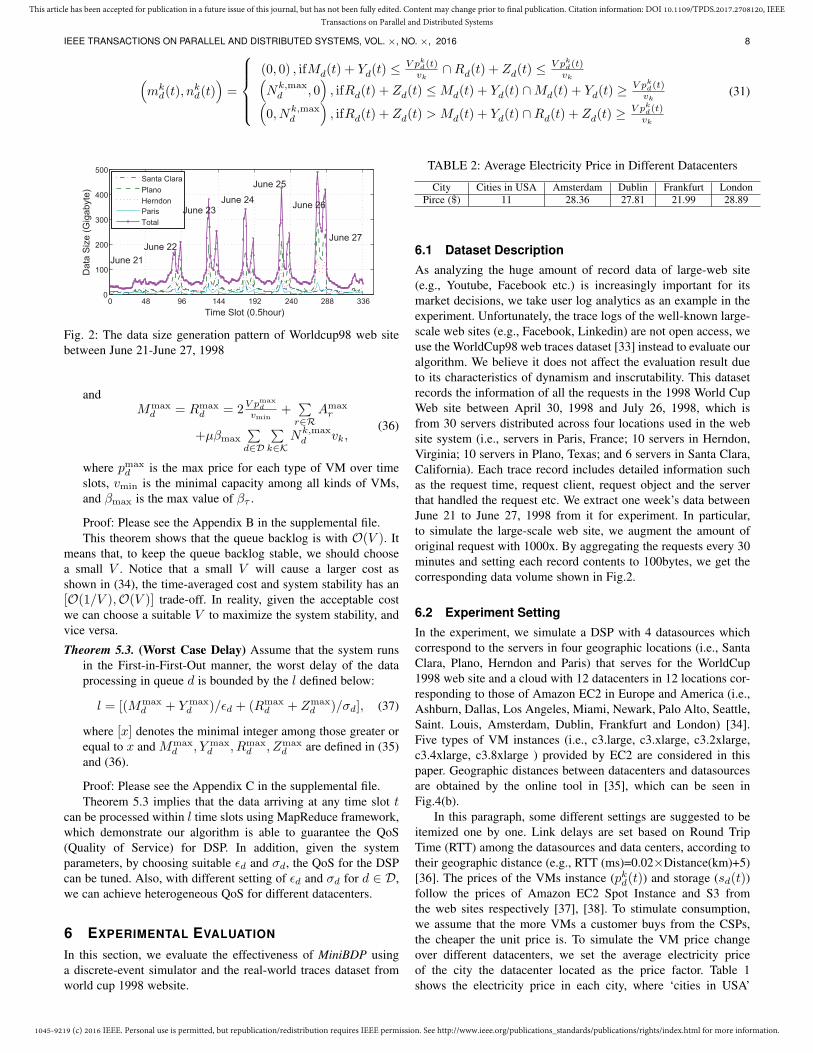
Fig. 2: The data size generation pattern of Worldcup98 web sitebetween June 21-June 27, 1998

andMmax

d = Rmaxd = 2

V pmaxd

vmin+

∑r∈R

Amaxr

+µβmax

∑d∈D

∑k∈K

Nk,maxd vk,

(36)

where pmaxd is the max price for each type of VM over time

slots, vmin is the minimal capacity among all kinds of VMs,and βmax is the max value of βτ .

Proof: Please see the Appendix B in the supplemental file.This theorem shows that the queue backlog is with O(V ). It

means that, to keep the queue backlog stable, we should choosea small V . Notice that a small V will cause a larger cost asshown in (34), the time-averaged cost and system stability has an[O(1/V ),O(V )] trade-off. In reality, given the acceptable costwe can choose a suitable V to maximize the system stability, andvice versa.

Theorem 5.3. (Worst Case Delay) Assume that the system runsin the First-in-First-Out manner, the worst delay of the dataprocessing in queue d is bounded by the l defined below:

l = [(Mmaxd + Y max

d )/ϵd + (Rmaxd + Zmax

d )/σd], (37)

where [x] denotes the minimal integer among those greater orequal to x and Mmax

d , Y maxd , Rmax

d , Zmaxd are defined in (35)

and (36).

Proof: Please see the Appendix C in the supplemental file.Theorem 5.3 implies that the data arriving at any time slot t

can be processed within l time slots using MapReduce framework,which demonstrate our algorithm is able to guarantee the QoS(Quality of Service) for DSP. In addition, given the systemparameters, by choosing suitable ϵd and σd, the QoS for the DSPcan be tuned. Also, with different setting of ϵd and σd for d ∈ D,we can achieve heterogeneous QoS for different datacenters.

6 EXPERIMENTAL EVALUATION

In this section, we evaluate the effectiveness of MiniBDP usinga discrete-event simulator and the real-world traces dataset fromworld cup 1998 website.

TABLE 2: Average Electricity Price in Different Datacenters

City Cities in USA Amsterdam Dublin Frankfurt LondonPirce ($) 11 28.36 27.81 21.99 28.89

6.1 Dataset DescriptionAs analyzing the huge amount of record data of large-web site(e.g., Youtube, Facebook etc.) is increasingly important for itsmarket decisions, we take user log analytics as an example in theexperiment. Unfortunately, the trace logs of the well-known large-scale web sites (e.g., Facebook, Linkedin) are not open access, weuse the WorldCup98 web traces dataset [33] instead to evaluate ouralgorithm. We believe it does not affect the evaluation result dueto its characteristics of dynamism and inscrutability. This datasetrecords the information of all the requests in the 1998 World CupWeb site between April 30, 1998 and July 26, 1998, which isfrom 30 servers distributed across four locations used in the website system (i.e., servers in Paris, France; 10 servers in Herndon,Virginia; 10 servers in Plano, Texas; and 6 servers in Santa Clara,California). Each trace record includes detailed information suchas the request time, request client, request object and the serverthat handled the request etc. We extract one week’s data betweenJune 21 to June 27, 1998 from it for experiment. In particular,to simulate the large-scale web site, we augment the amount oforiginal request with 1000x. By aggregating the requests every 30minutes and setting each record contents to 100bytes, we get thecorresponding data volume shown in Fig.2.

6.2 Experiment SettingIn the experiment, we simulate a DSP with 4 datasources whichcorrespond to the servers in four geographic locations (i.e., SantaClara, Plano, Herndon and Paris) that serves for the WorldCup1998 web site and a cloud with 12 datacenters in 12 locations cor-responding to those of Amazon EC2 in Europe and America (i.e.,Ashburn, Dallas, Los Angeles, Miami, Newark, Palo Alto, Seattle,Saint. Louis, Amsterdam, Dublin, Frankfurt and London) [34].Five types of VM instances (i.e., c3.large, c3.xlarge, c3.2xlarge,c3.4xlarge, c3.8xlarge ) provided by EC2 are considered in thispaper. Geographic distances between datacenters and datasourcesare obtained by the online tool in [35], which can be seen inFig.4(b).

In this paragraph, some different settings are suggested to beitemized one by one. Link delays are set based on Round TripTime (RTT) among the datasources and data centers, according totheir geographic distance (e.g., RTT (ms)=0.02×Distance(km)+5)[36]. The prices of the VMs instance (pkd(t)) and storage (sd(t))follow the prices of Amazon EC2 Spot Instance and S3 fromthe web sites respectively [37], [38]. To stimulate consumption,we assume that the more VMs a customer buys from the CSPs,the cheaper the unit price is. To simulate the VM price changeover different datacenters, we set the average electricity priceof the city the datacenter located as the price factor. Table 1shows the electricity price in each city, where ‘cities in USA’




0 50 100 150 200 250 300 3500

200

400

600

800

1000

1200

1400

Time slot

Cost ($

)

V=60, γ=0.5, α=0.01

(a) Cost incurred over time slots

0 50 100 150 200 250 300 3500

0.2

0.4

0.6

0.8

1

Time slot

Cost R

atio o

f each V

M T

ype

large xlarge 2xlarge 4xlarge 8xlarge

(b) CR of each type of VM over time slots

0 50 100 150 200 250 300 3500

0.2

0.4

0.6

0.8

Time Slot

Co

st

Ratio Porcess Cost

Storage Cost

Bandwidth Cost

Latency Cost

Migration Cost

(c) CR of each type of cost over time slots

Fig. 3: Cost metric over time slots

0.0

868.3

2720.1

150.1

94.3

3419.9

451.7

0.0

1796.1

1197.6

192.8

0.0

0.0

1590.6

1442.6

60.3

0.0

1012.2

1956.4

294.4

1928.3

911.5

109.9

11.5

1426.6

1021.4

353.8

2.9

64.0

2043.1

1343.4

28.5

0.0

52.1

0.0

493.7

0.0

75.8

0.0

469.5

0.0

60.6

0.0

955.6

0.0

0.0

56.0

515.0

Ashburn

Dallas

Los Angeles

Miam

i

New

ark

Palo A

lto

Seattle

Saint. Louis

Am

sterdam

Dublin

Frankfurt

London

Santa Clara

Plano

Herndon

Paris

0 500 1000 1500 2000 2500 3000

Unit: Gigabyte

(a) Amount of data allocated from datasources todatacenters

3855

1850

12

6192

2340

28

1877

7943

497

1998

3665

9095

4128

1790

1493

7364

4097

2174

337

5853

19

2357

3879

8981

1141

2693

3710

8050

2775

856

1111

7061

8803

7882

6213

430

8201

7159

5466

781

9164

8238

6555

478

8643

7623

5922

343

Ashburn

Dallas

Los Angeles

Miam

i

New

ark

Palo A

lto

Seattle

Saint. Louis

Am

sterdam

Dublin

Frankfurt

London

Santa Clara

Plano

Herndon

Paris

1000 2000 3000 4000 5000 6000 7000 8000 9000

Unit: Km

(b) Geographical distance from datasources to datacen-ters

0

10

20

30

40

50

60

Reducer

Sle

ction T

imes

Ashburn

Dallas

Los Angele

s

Mia

mi

Newark

Palo A

lto

Seattle

Saint.

Louis

Amst

erdam

Dublin

Frankf

urt

London

(c) Reducer Selection times of each datacen-ter

Fig. 4: Statistic metric of decision λ and x

include Ashburn, Dallas, Los Angeles, Miami, Newark, Palo Alto,Seattle, Saint. Louis. As suggested by [7], the unit charge ofuploading data to datacenters via link < r, d > is within [0.10,0.25]$/GB and the migration cost function is set as a linearfunction on the amount of data migrated, with a price of inter-datacenter bandwidth in the range of [0.10, 0.25]$/GB. We setthe uplink bandwidth capacity Ud

r is with uniform distributionwithin [30, 50]M/s. For the involvement of historical data, wereuse the past 2 time slots’ intermediate data at current timeslot (i.e., βt−1 > βt−2 > βt−3 = ... = 0). Unless indicatedotherwise, the default experiment setting is adopted as follows:V = 60, γ = 0.5, α = 0.01, ϵd = 1, σd = γ × ϵd.

Performance Metrics: In the experiments, two metrics costand queue size are mainly considered. Cost measures the economicaspects of the system while queue size describes the stability ofthe system. To facilitate the comparison, Cost Ratio (CR), whichmeasures the cost proportion of a single case among the totalcost obtained by all cases, is used in the experiments. It can be

calculated by using CRcur = Ccur/N∑i=1

Ci, where Ci denotes

the cost incurred by the i-th case and N is the case count..

6.3 Performance under Fixed Setting

In this section, we conducted a group of experiments under fixedparameters (the values set for these parameters can be seen insubsection 6.2) to evaluate the effectiveness of MiniBDP. Fig.3(a)presents the total cost of the system incurred over time slots.It can be observed that the cost fluctuates synchronously withthe data generation pattern as shown in Fig.2, which means thatMiniBDP is able to adaptively lease and adjust VMs resources tomeet dynamic data processing demands even in a flash-crowdedstyle without forecasting the future workload information. This

is substantially different from those existing methods that needprediction phase in algorithm design. Fig.3(b) illustrates the CRcomparisons among different VM types, from which we find thatthe larger the VM capacity is, the more the number of VM withthe corresponding type will be rented. This is probably becausewe design the pricing strategy with the principle that the morecapacity of the VM is, the lower the unit price of the VM is. Thus,the algorithm prefers to rent the VM instance with large capacity(e.g.,c3.8xlarge ) to process the data. The cost components (i.e.,processing cost, storage cost, bandwidth cost, latency cost, andmigration cost) at each time slot are also compared in Fig.3(c),which shows that processing cost occupies the major part of thetotal cost and the other types of cost are relatively low. This revealsthat the algorithm is able to select the suitable datacenter for dataprocessing while reducing the extra cost.

Furthermore, to exploit the inner property of the algorithm,details of decision on data allocation and reducer selection arepresented. Fig.4(a) shows the data allocation matrix map fromdatasources to datacenters and Fig.4(b) illustrates the correspond-ing geographic distance map. As can be observed, the algorithmshows data locality property since data are preferred to be movedto the near datacenter for processing. The remoter the datacenteris, the less the data are moved to. In particular, there is hardlyany data should be moved from Paris to the datacenters in NorthAmerica (i.e., Ashburn, Dallas, Los Angeles, Miami, Newark,Palo Alto, Seattle, Saint. Louis) even the price in the Europe issignificantly higher than that in the North America. This meansthat our algorithm is capable of avoiding long latency cost toguarantee the data processing delay. Fig.4(c) depicts the timesof reducer selection of each datacenter, which also shows thatmajority of the Reduce operations are done within the datacenterslocated in the North America. With this strategy, the migration




0 50 100 150 200250

300

350

400

450

500T

ime A

vera

ged C

ost ($

)

V0 50 100 150 200

100

200

300

400

500

600

Tim

e A

vera

ged

Queue S

ize (

Gig

abyte

)Cost

Queue Size

(a) Impact of V on cost and queue size

0.5 1 1.5 2200

300

400

500

600

700

800

Tim

e A

vera

ged C

ost ($

)

γ0.5 1 1.5 2

200

250

300

350

400

450

500

550

600

650

Tim

e A

vera

ged

Queue S

ize (

Gig

abyte

)

Cost

Queue Size

(b) Impact of γ on cost and queue size

0 5 10 15340

360

380

400

420

440

460

480

500

Tim

e A

ve

rag

ed

Co

st

($)

0 5 10 1590

110

130

150

170

190

210

230

250

270

Tim

e A

ve

rag

ed

Q

ue

ue

Siz

e (

Gig

ab

yte

)

ε

Cost

Queue Size

(c) Impact of ϵ on cost and queue size

Fig. 5: Impact of important parameters on cost and queue size

0 0.02 0.04 0.06 0.08 0.1

0

0.2

0.4

0.6

0.8

1

α

Cost R

atio

Total Cost

Process Cost

Storage Cost

Bandwidth Cost

Latency Cost

Migration Cost

(a) Impact of α on cost

0

100

200

300

400

500

600

700

Tim

e A

ve

rag

ed

Co

st

($)

MiniB

DP

SVP+PDA+MCRS

SVP+PDA+LBRS

SVP+LBDA+MCRS

SVP+LBDA+LBRS

SVP+MPDA+M

CRS

SVP+MPDA+LBRS

HVP+PDA+MCRS

HVP+PDA+LBRS

HVP+LBDA+MCRS

HVP+LBDA+LBRS

HVP+MPDA+M

CRS

HVP+MPDA+LBRS

(b) Cost comparison with other strategies

0 50 100 150 200 250 300 3500

500

1000

1500

2000

2500

3000

3500

Time slot

Avera

ge

Work

loa

d Q

ue

ue B

acklo

g

MiniBDP

SVP+PDA+MCRS

SVP+PDA+LBRS

SVP+LBDA+MCRS

SVP+LBDA+LBRS

SVP+MPDA+MCRS

SVP+MPDA+LBRS

HVP+PDA+MCRS

HVP+PDA+LBRS

HVP+LBDA+MCRS

HVP+LBDA+LBRS

HVP+MPDA+MCRS

HVP+MPDA+LBRS

(c) Queue size comparison with other strategies

Fig. 6: Comparison with other strategies

cost is reduced since migrating the data from 4 datacenters locatedin the Europe to 8 datacenters in the North America is moreeconomic than in the opposite route.

6.4 Impact of Parameters

In this section, we investigate the impact of important parameters(i.e., V, γ, ϵ, α) on the algorithm.

(1) As presented previously, V is a very important parameterto the model, which controls the trade-off between cost and queuesize. Fig.5(a) depicts the cost and workload queue size (i.e.,Md(t) + Rd(t)) curve with the variation of V , from which wecan observe that the time-averaged cost incurred by the systemdeclines with the increase of V and converges to a minimumvalue with the increase of V . This provides a guidance for usto reduce the total cost when implementing a real-world system.However, the workload queue size increases with the increase ofV . It may lead to the increase of data processing latency since thelonger the queue is, the more time it needs to wait for processing.Furthermore, this experimental result is also consistent with thetheoretical analysis result of the algorithm in Theorem 5.1 andTheorem 5.2. With this property, given a cost budget, we canchoose a suitable V for the system.

(2) The ratio between intermediate data size produced at Mapphase and the raw data size imported into Map (i.e., γ) is studied.As can be seen from Fig. 5(b), both cost and queue size growwith the increase of γ. Intuitively, the larger the γ is, the morethe intermediate data will be produced. Hence, more resources areneeded to process the intermediate data as well more cost willincur in data transportation and storage. When γ increases to alarge degree, the cost improves slightly. This may due to the factthat finite amount of VM resources in each datacenter are set, thusall of the VMs will be rented when the γ increases to a specificdegree, resulting in a slight change of cost.

(3) To validate the Theorem 5.3, we conduct experiments withthe variation of ϵ and σ that can be used to control the worst casequeue delay. For simplicity, we set the same ϵ and σ for all thedatacenters (i.e., ϵ1 = ... = ϵD = ϵ, σ1 = ... = σD = σ)and σ = γ × ϵ. Fig.5(c) illustrates the experimental results, inwhich we can observe that the cost increases while the queue sizedecreases with the increase of ϵ. This can be explained by the factthat, with the growth of ϵ and σ, the worst delay l declines (referto (37)). Therefore, it needs more VMs to process the data withina short delay, and thus resulting in a cost increase. Similarly,the queue length needs to be shortened to guarantee the dataprocessing delay when ϵ and σ increase. Hence, from this point ofview, the theoretical result of Theorem 5.3 is also validated.

(4) The impact of α is also studied by comparing the cost com-ponents fluctuation with the change of α. As exhibited in Fig.6(a),the cost of bandwidth and migration cost keep a low level, whichmeans MiniBDP is able to avoid unnecessary data moving acrossdatacenters. The graph also shows the costs of storage, bandwidthand migration vary slightly, while the processing cost decreasesand the latency cost increases obviously with the increase of α.This may because the costs of storage, bandwidth and migrationare mainly determined by the amount of data, and processing costdecreases since latency cost increases with α under a fixed V .Therefore, for a larger latency factor α, we should set a smaller Vto guarantee the processing delay.

6.5 Comparisons

In this section, we compare MiniBDP with other alternatives, eachof which is the combination of a data allocation strategy, VMprovisioning strategy and reducer selection strategy.

For the data allocation policies, three representative strate-gies are considered. 1) Proximity-aware Data Allocation (PDA),in which dynamically generated data from each datasource are




always allocated to the geographically nearest datacenter. Itproduces minimal latency and is suitable for the scenario thatlatency delay is prior to other factors. 2) Load-balancing DataAllocation (LBDA), in which the data from each datasource arealways dispatched to the datacenter with the lowest Map workload.Obviously, this strategy is capable of keeping workload balancedamong datacenters. 3) Minimal Price Data Allocation (MPDA),in which the data from each datasource are allocated to the mosteconomic datacenter, so as to achieve the lowest cost.

For the VM provisioning policies, two typical strategies areconsidered. 1) Heuristic VM Provisioning (HVP), in which theVMs needed at current time are estimated based on the workloadat previous time. To cope with the fluctuation of workload, extra50 percent VMs are added to those need at previous time to formthe final decision. 2) Stable VM Provisioning (SVP), in whichthe VM count of each type in each datacenter is set to a fixedvalue. For ease of comparison, we configure the fixed value as theaverage VM of each type achieved by MiniBDP. Thus, the amountof VMs consumed by SVP is equal to that of MiniBDP within timeperiod T .

For the reducer selection strategies, we consider two approach-es as follows. 1) Minimal Migration Cost Reducer Selection(MCRS), this takes the migration cost priority to select the reducer.2) Load Balance Reducer Selection (LBRS), which selects thedatacenter with the smallest workload of Reduce as the reducer.

Therefore, combining with the aforementioned strategies,we have following approaches: MiniBDP, SVP+PDA+MCRS,SVP+PDA+LBRS, SVP+LBDA+MCRS, SVP+LBDA+LBRS,SVP+MPDA+MCRS, SVP+MPDA+LBRS, HVP+PDA+MCRS,HVP+PDA+LBRS, HVP+LBDA+MCRS, HVP+LBDA+LBRS,HVP+MPDA+MCRS, HVP+MPDA+LBRS.

Fig.6(b) presents comparison of the time-averaged cost in-curred by different strategies. From this graph, we have followingobservations: (1) Our algorithm MiniBDP outperforms the major-ity of others except SVP+PDA+MCRS and SVP+PDA+LBRS interms of cost. This is because these two strategies only move thedata to the geographically nearest datacenter, resulting in lowestbandwidth cost and latency cost. Notwithstanding, this strategy isnot really effective since their corresponding queue size increaseswith the increase of time slots (as shown in Fig.6(c)), which meansthat the system can not keep stable in the long run. As analyzedin section 6.3, MiniBDP also has the property of data locality.Hence, compared with these two strategies, MiniBDP makes anbetter trade-off between data locality and system stability. (2)HVP+LBDA+MCRS and HVP+LBDA+LBRS incur the highestcost. We believe it may due to their load-balanced data allocationstrategy in which moving large amount of data from USA to Pariswithout considering the high bandwidth cost and latency cost oncross-ocean links. From Fig.6(c), it can be seen that only MiniBDPis stable in queue size even after running a long time. Whereas,the queue size of other strategies exhibit to be increasing with thetime axis, which will certainly lead to the fail of system. Notethat SVP provisions the same number of VM with MiniBDP whilecausing higher cost and system instability, it can be concluded thatMiniBDP is capable of optimizing the three decisions to reduce thetotal cost. As mentioned previously, the VM of HVP is provisionedby adding extra 50 percent VMs to those needed at previous timeslots. However, those using this VM provisioning strategy in factdo not work well since the queue size of the system is not stable.

Combining Fig.6(b) and Fig.6(c), it seems some sim-ple strategies (e.g., SVP+LBDA+LBRS, SVP+MPDA+LBRS,

0 50 100 150 200 250 300 3500

500

1000

1500

CP

U t

ime

(S

eco

nd

)

0 50 100 150 200 250 300 3500

0.5

1

1.5

2

Time slot

Optimal−2slot

Optimal−4slot

MiniBDP

Optimal−1slot

Fig. 7: Solving time Comparison with optimal

HVP+PDA+LBRS) are close to MiniBDP. In fact, these strategiesdo not perform very well for a long period since the queue sizesshow increasing trends. Furthermore, since the number of VMs instrategy SVP is obtained based on the result of MiniBDP, SVP isactually unreachable in reality.

In addition, we also compare MiniBDP with the offline optimalones. Since the original problem contains 60480 variables (at onetime slot, m, n are with 60 variables, x is with 12 variables, λ iswith 48 variables, thus for 336 time slots, there are 180 × 336variables), existing optimization toolboxes (e.g., GLPK ,CPLEX,LPSOLVE, etc.) show failed to solve such an extreme large-scaleinteger nonlinear optimization on a Spur server with Intel(R) X-eon(R) CPU (1.90GHz), 128GB RAM, 64bits Windows operationsystem. Thus, we divide the long time slots into several partswith an interval and solve each of them instead using BMIBNBwith lower solver CPLEX, upper solver FMINCON in Matlab. Infact, these alternatives are with known data arrival and achievesuboptimal offline solutions. Furthermore, the tolerable delays arealso fixedly set as interval time slots since the data must beprocessed within interval time slot. In this experiment, differentintervals are set to study its performance. Fig.8 depicts thecumulative cost comparison along time slots (Optimal-xslot meansthat the interval is x), which shows that MiniBDP performs betterthan the cases interval = 1, interval = 2 and interval = 4and the larger the interval is, the lower the cost is incurred. Webelieve this is because: 1) data processing must be completedwithin 1, 2, 4 time slots for Optimal-1slot, Optimal-2slot andOptimal-4slot, respectively and, 2) a smaller interval needs moreVM resource to complete data processing due to its short delay.Whereas, MiniBDP has a soft delay control mechanism by settingthe ϵ and σ, the cost will be reduced by setting a long tolerabledelay. The time used for solving the problem is compared inFig.7, which shows that it requires only about 0.15 seconds forMiniBDP to make decision since it is based on some simplestrategies, thus it can run in an online fashion. However, theCPU time consumed by Optimal-2slot (average 83.9 seconds),Optimal-4slot (average 523.8 seconds) is significantly higher thanthat of MiniBDP because it needs extensive searching time tofind the global optimal. Note that Optimal-1slot runs relativelyfast (only needs 0.4 seconds), this may attribute to the fact thatthe problem comes into a mixed integer linear optimization thatcan be efficiently solved by existing tools (e.g., LPSOLVE) wheninterval = 1 since the migration data produced at former time




0 50 100 150 200 250 300 3500

5

10

15x 10

4

Time Slot

Cum

ula

tive C

ost ($

) MiniBDP

Optimal−1slot

Optimal−2slot

Optimal−4slot

(a) Cumulative cost comparisonFig. 8: Cost Comparison with Optimal

0

2000

4000

6000

8000

10000

Data

Allo

cate

d to

Data

cente

r (G

igabyte

)

Ashburn

Dallas

Los Angele

s

Mia

mi

Newark

Palo A

lto

Seattle

Saint.

Louis

Amst

erdam

Dublin

Frankf

urt

London

Optimal−1slot

(a) Data allocation result of Optimal-1slot

0

100

200

300

400

Reducer

Sle

ction T

imes

Ashburn

Dallas

Los Angele

s

Mia

mi

Newark

Palo A

lto

Seattle

Saint.

Louis

Amst

erdam

Dublin

Frankf

urt

London

Optimal−1slot

(b) Reducer slection result of Optimal-1slota

Fig. 9: Solution of Optimal-1slot

slot is known (i.e., hi(t) is known, no xd(t) ∗mkd(t) term exists).

We also find that the solving time increases exponentially withthe interval, e.g., we run Optimal-2slot for nearly 8.5 hours andOptimal-4slot for more than two days, thus to optimize the originalproblem in an online manner is almost infeasible. Finally, as canbe seen in Fig.9, the solution of Optimal-1slot is not able to keepthe load balancing among datacenters since it mainly allocates datato only five datacenters and runs reducer in only 1 datacenters. Sodo the the solutions of Optimal-2slot and Optimal-2slot, we omitthem here due to page limit. Therefore, MiniBDP with simplestrategies shows many advantages over offline optimal solutionand a real-world implementation prospect.

7 CONCLUSION AND FUTURE WORK

With high velocity and high volume of big data generated fromgeographically dispersed sources, big data processing across ge-ographically distributed datacenters is becoming an attractive andcost effective strategy for many big data companies and organi-zations. In this paper, a methodical framework for effective datamovement, resource provisioning and reducer selection with thegoal of cost minimization is developed. We balance five typesof cost: bandwidth cost, storage cost, computing cost, migrationcost, and latency cost, between the two MapReduce phases acrossdatacenters. This complex cost optimization problem is formulatedinto a joint stochastic integer nonlinear optimization problem byminimizing the five cost factors simultaneously. By employingLyapunov technique, we transform the original problem into threeindependent subproblems that can be solved by designing anefficient online algorithm MiniBDP to minimize the long-termtime-average operation cost. We conduct theoretical analysis todemonstrate the effectiveness of MiniBDP in terms of cost opti-mum and worst case delay. We perform experimental evaluationusing real-world trace dataset to validate the theoretical result andthe superiority of MiniBDP by compared it with existing typicalapproaches and offline methods.

The proposed approach is predicted to be with widespreadapplication prospects in those globally-serving companies sinceanalyzing the geographically dispersed datasets is an efficient wayto support their marketing decision. As the subproblems in thealgorithm MiniBDP are with analytical or efficient solutions thatguarantee the algorithm running in an online manner, the proposedapproach can be easily implemented in the real system to reducethe operation cost. In the future work, we will focus on followingaspects: 1) Extending the original model to support other typesof jobs. Note the approach is designed mainly for data warehouse

type of job such as statistic analysis and SQL query and someother kinds data processing (e.g., astronomic image processing),the graph type of jobs and the jobs with iteration property are notoriginally supported in the paper due to the streaming propertyof the queue designs. However, the proposed approach can beextended to adapt to these cases with minor extensions. E.g., if wechange the original model by adding a self-circulation data flowat the data allocation stage and designing a coordinator to transferthe reduce result to mappers, the iterative jobs can be supported.2) Taking into consideration the factor of data replication in themodel. Data replication is well-known as an effective solution forhigh availability and high fault tolerance. Given that our goal iscost minimization, introducing data replication will add additionalcost of replicating data across datacenters. Thus, this factor is notconsidered in our current cost minimization algorithm and we leftit to be one of our ongoing research efforts. 3) In addition, wewill concentrate on deploying the proposed algorithm in the realsystems such as Amazon EC2 to further validate its effectiveness.

ACKNOWLEDGEMENT

This research is supported by the National Natural ScienceFoundation of China under grant 61572511, the Natural ScienceFoundation of Hunan Province under grant 2015JJ3023 as well asthe Overseas, Hongkong&Macau Scholars Collaborated ResearchFund of China under grant 11428101 as well as the ScientificResearch Project of National University of Defense Technologyunder grants ZK16-03-57 and ZK16-03-09.

REFERENCES

[1] “Square kilometre array,” http://www.skatelescope.org/.[2] A. Vulimiri, C. Curino, B. Godfrey, T. Jungblut, J. Padhye, and G. Vargh-

ese, “Global analytics in the face of bandwidth and regulatory con-straints,” in Proceedings of the USENIX NSDI’15, 2015.

[3] J. Dean and S. Ghemawat, “Mapreduce: Simplified data processing onlarge clusters,” Communications of the ACM, vol. 51, no. 1, pp. 107–113,2008.

[4] M. Zaharia, M. Chowdhury, M. J. Franklin, S. Shenker, and I. Stoica,“Spark: Cluster computing with working sets,” in Proceedings of theUSENIX HotCloud’10, 2010.

[5] E. E. Schadt, M. D. Linderman, J. Sorenson, L. Lee, and G. P.Nolan,“Computational solutions to large-scale data management and analysis,”Nature Reviews Genetics, vol. 11, no. 9, pp. 647–657, 2010.

[6] M. Cardosa, C. Wang, A. Nangia et al., “Exploring mapreduce efficiencywith highly-distributed data,” in Proceedings of the second internationalworkshop on MapReduce and its applications, 2011.

[7] L. Zhang, C. Wu, Z. Li, C. Guo, M. Chen, and F. C. M. Lau, “Moving bigdata to the cloud: An online cost-minimizing approach,” IEEE Journalon Selected Areas in Communications, vol. 31, pp. 2710–2721, 2013.




[8] W. Yang, X. Liu, L. Zhang, and L. T. Yang, “Big data real-timeprocessing based on storm,” in Proceedings of the IEEE TrustCom’13,2013.

[9] Y. Zhang, S. Chen, Q. Wang, and G. Yu, “i2mapreduce: Incrementalmapreduce for mining evolving big data,” IEEE Transactions on Knowl-edge and Data Engineering, vol. 27, pp. 1906–1919, 2015.

[10] D. Lee, J. S. Kim, and S. Maeng, “Large-scale incremental processingwith mapreduce,” Future Generation Computer Systems, vol. 36, no. 7,pp. 66–79, 2014.

[11] B. Heintz, A. Chandra, R. K. Sitaraman, and J. Weissman, “End-to-end optimization for geo-distributed mapreduce,” IEEE Transactions onCloud Computing, 2014.

[12] C. Jayalath, J. Stephen, and P. Eugster, “From the cloud to the atmo-sphere: Running mapreduce across data centers,” IEEE Transactions onComputers, vol. 63, no. 1, pp. 74–87, 2014.

[13] P. Li, S. Guo, S. Yu, and W. Zhuang, “Cross-cloud mapre-duce for big data,” IEEE Transactions on Cloud Computing, 2015,dOI:10.1109/TCC.2015.2474385.

[14] A. Sfrent and F. Pop, “Asymptotic scheduling for many task computingin big data platforms,” Information Sciences, vol. 319, pp. 71–91, 2015.

[15] L. Zhang, Z. Li, C. Wu, and M. Chen, “Online algorithms for uploadingdeferrable big data to the cloud,” in Proceedings of the IEEE INFOCOM,2014, pp. 2022–2030.

[16] Q. Zhang, L. Liu, A. Singhand et al., “Improving hadoop serviceprovisioning in a geographically distributed cloud,” in Proceedings ofIEEE Cloud’14, 2014.

[17] A. Vulimiri, C. Curino, P. B. Godfrey, K. Karanasos, and G. Varghese,“Wanalytics: Analytics for a geo-distributed data-intensive world,” inProceedings of the CIDR’15, 2015.

[18] K. Kloudas, M. Mamede, N. Preguica, and R. Rodrigues, “Pixida:Optimizing data parallel jobs in wide-area data analytics,” Proceedingsof the VLDB Endowment, vol. 9, no. 2, pp. 72–83, 2015.

[19] Q. Pu, G. Ananthanarayanan, P. Bodik, S. Kandula, A. Akella, P. Bahl,and I. Stoica, “Low latency geo-distributed data analytics,” in Proceed-ings of the ACM SIGCOMM’15, 2015.

[20] “Facebook’s prism project,” http://www.wired.com/wiredenterprise/2012/08/facebook-prism/.

[21] J. C. Corbett, J. Dean, M. Epstein et al., “Spanner: Google’s globally-distributed database,” in Proceedings of the OSDI’12, 2012.

[22] “Connecting geographically dispersed datacenters,” HP, 2015.[23] “Interconnecting geographically dispersed data centers using vpls-design

and system assurance guide,” Cisco Systems, Inc, 2009.[24] L. Tassiulas and A. Ephremides, “Stability properties of constrained

queueing systems and scheduling policies for maximum throughput inmultihop radio networks,” IEEE Transactions on Automatic Control,vol. 37, no. 12, pp. 1936–1948, 1992.

[25] R. Urgaonkar, U. C. Kozat, K. Igarashi, and M. J. Neely, “Dynamicresource allocation and power management in virtualized data centers,”in Proceedings of the IEEE NOMS, 2010, pp. 479–486.

[26] F. Liu, Z. Zhou, H. Jin, B. Li, B. Li, and H. Jiang, “On arbitratingthe power-performance tradeoff in saas clouds,” IEEE Transactions onParallel and Distributed Systems, vol. 25, no. 10, pp. 2648–2658, 2014.

[27] Y. Yao, L. Huang, A. Sharma, L. Golubchik, and M. Neely, “Powercost reduction in distributed data centers: A two-time-scale approach fordelay tolerant workloads,” IEEE Transactions on Parallel and DistributedSystems, vol. 25, no. 1, pp. 200–211, 2014.

[28] D. Wu, Z. Xue, and J. He, “icloudaccess: Cost-effective streaming ofvideo games from the cloud with low latency,” IEEE Transactions onCircuits and Systems for Video Technology, vol. 24, no. 8, pp. 1405–1416, 2014.

[29] W. Xiao, W. Bao, X. Zhu, C. Wang, L. Chen, and L. T. Yang, “Dynamicrequest redirection and resource provisioning for cloud-based video ser-vices under heterogeneous environment,” IEEE Transactions on Paralleland Distributed Systems, vol. 27, no. 7, pp. 1954–1967, 2016.

[30] S. Rao, R. Ramakrishnan, A. Silberstein et al., “Sailfish: a framework forlarge scale data processing,” in Proceedings of the Third ACM Symposiumon Cloud Computing, 2012.

[31] M. Neely, Stochastic Network Optimization with Application to Commu-nication and Queueing Systems. Morgan and Claypool, 2010.

[32] M. J. Neely, “Opportunistic scheduling with worst case delay guaranteesin single and multi-hop networks,” in Proceedings of the IEEE INFO-COM, 2011, pp. 1728–1736.

[33] M. Arlitt and T. Jin, “A workload characterization study of the 1998world cup web site,” IEEE Network, vol. 14, no. 3, pp. 30–37, 2000.

[34] “Where amazon’s data centers are located,”http://www.datacenterknowledge.com/archives/2008/11/18/where-amazons-data-centers-are-located/.

[35] “Gpsspg,” http://www.gpsspg.com/distance.htm.[36] A. Qureshi, “Power-demand routing in massive geo-distributed systems,”

Ph.D. dissertation, Massachusetts Institute of Technology, 2010.[37] “Amazon elastic compute cloud,” http://aws.amazon.com/ec2/.[38] “Amazon simple storage service,” http://aws.amazon.com/s3/.

Wenhua Xiao received his B.S. and M.S. de-gree from the International School of Softwareat Wuhan University, China, in 2010 and Collegeof Information and System Management at Na-tional University of Defense Technology (NUDT),China, in 2012 respectively. He is currently aPh.D. student in the College of Information Sys-tem and Management at NUDT. His researchinterests include scheduling, resource manage-ment in cloud computing and big data.

Weidong Bao received his Ph.D. degree in man-agement science and engineering from the Na-tional University of Defense Technology in 1999.He is currently a Professor in the College ofInformation Systems and Management at Na-tional University of Defense Technology, Chang-sha, China. His recent research interests includecloud computing, information system, and com-plex network. He has published more than 50research articles in refereed journals and con-ference proceedings such as IEEE Transactions

on Computers, IEEE Transactions on Parallel and Distributed Systemsand so on. He was a visiting scholar at Arizona State University fromMay 2013 to May 2014. He serves on the editorial board of AIMS BigData and Information Analytics.

Xiaomin Zhu received the the PhD degree incomputer science from Fudan University, Shanghai, China, in 2009. In the same year, he re-ceived the Shanghai Excellent Graduate Award.He is currently an Associate Professor in the Col-lege of Information Systems and Managementat National University of Defense Technology,Changsha, China. His research interests includescheduling and resource management in greencomputing, cluster computing, cloud computing,and multiple satellites. He has published more

than 70 research articles in refereed journals and conference proceed-ings such as IEEE Transactions on Computers, IEEE Transactions onParallel and Distributed Systems, Journal of Parallel and DistributedComputing, Journal of Systems and Software, and so on. He was avisiting scholar at York University and Georgia Institute of Technologyfrom June 2014 to September 2014 and September 2015 to September2016, respectively. He serves on the editorial board of Future Genera-tion Computer Systems and AIMS Big Data and Information Analytics.He is a member of the IEEE, the IEEE Communication Society, and theACM.

Ling Liu is a Professor in the School of Com-puter Science at Georgia Institute of Technology.She directs the research programs in DistributedData Intensive Systems Lab (DiSL). She haspublished over 300 international journal and con-ference articles and is a recipient of the bestpaper award from a number of top venues, in-cluding ICDCS 2003, WWW 2004, 2005 PatGoldberg Memorial Best Paper Award, IEEECloud 2012, IEEE ICWS 2013, IEEE/ACM CC-Grid 2015. She is an elected IEEE Fellow. She

is the editor in chief of IEEE Transactions on Service Computing, andserves on the editorial board of international journals, including ACMTransactions on Web (TWEB), ACM Transactions on Internet Technolo-gy (TOIT).

ieee transactions on parallel and … · cost-aware big data processing across geo-distributed...

Documents