IEEE TRANSACTIONS ON NUCLEAR SCIENCE, VOL. 62, NO. 1, FEBRUARY 2015 131

Revisit of the Ramp FilterGengsheng L. Zeng, Fellow, IEEE

Abstract—An important part of the filtered backprojection(FBP) algorithm is the ramp filter. This paper derives the discreteversion of the ramp filter in the Fourier domain and studies thewindowing effects. When a window function is used to controlthe noise, the image amplitude will be affected and reduced. Asimple remedy is proposed to improve the image accuracy whena window function must be used.

Index Terms—Analytic image reconstruction, filtered backpro-jection algorithm.

I. INTRODUCTION

T HE filtered backprojection (FBP) algorithm has beenserving as the driving engine in tomographic image re-

construction for many decades [1]–[4]. This algorithm consistsof ramp filtering and backprojeciton procedures. Ramp filteringcan be implemented as convolution in the spatial domain ormultiplication in the Fourier domain.The continuous ramp filter has a zero DC gain. Therefore, if

one directly samples the continuous ramp filter to obtain a dis-crete version, the discrete version will also have a zero DC gain.It has been shown that this zero DC gain can cause a reconstruc-tion bias error [5]–[7]. In fact, this error can be easily correctedby using a non-zero DC gain in the sampled ramp filter. Thispaper will give a systematic treatment of the issue and give arelationship between a continuous filter’s transfer function andits exact discrete counterpart.This paper will use the discrete/periodic duality [8] to derive

an exact explicit expression for the discrete ramp filter. The dis-crete/periodic duality is a fundamental property for a Fouriertransform pair. If a function is periodic in one domain, it is dis-crete in the other domain, and vice versa. Since the projectionsare to be filtered in the discrete Fourier domain, an exact cir-cular convolution expression in the spatial domain must be ob-tained first. A circular convolution is nothing but a linear convo-lution with two periodic functions; these two functions have thesame period. If these two periodic functions are also discrete, thecircular convolution can be calculated via the Discrete FourierTransform (DFT). The DFT can be efficiently computed by theFast Fourier Transform (FFT).In general, the FFT method is faster than the convolution

method. However, in some special cases, the convolution

Manuscript received May 07, 2014; revised August 01, 2014; accepted Oc-tober 15, 2014. Date of publication October 30, 2014; date of current versionFebruary 06, 2015. This work was supported in part by the U.S. National Insti-tute of Health under Grant NIH 1R01HL108350.The author is with the Department of Electrical Engineering, Weber State

University, Ogden, UT 84408 USA and also with the Department of Radiology,University of Utah, Salt Lake City, UT 84108 USA (e-mail: larryzeng@weber.edu).Digital Object Identifier 10.1109/TNS.2014.2363776

method can be faster, for example, when the filter is spatiallyvarying. The backprojection is still the dominating procedurein terms of computation cost.Noise control in the FBP algorithm is achieved by the appli-

cation of a window function, which is normally a low-pass filterwith a unity DC gain. The window function can affect the accu-racy of the FBP reconstruction. This effect has been ignored forthe purpose of simplification in image analysis [9]. This paperwill investigate how the window function can reduce the ampli-tude of the reconstructed image and propose a simple remedy.

II. METHODS

A. Converting a Continuous Filter Into a Discrete Filter

Linear filtering can be achieved either by convolution with aspatial domain kernel function (i.e., a convolver) or by multi-plication with a Fourier domain transfer function. The transferfunction is the Fourier transform of the spatial domain kernelfunction.First of all, it is generally incorrect to obtain a discrete transfer

function by sampling a continuous transfer function. Let theprojection at a certain view angle be ,where is theindex along the detector. The projection is discretely sam-pled and has a finite support . Without loss of generality, thesampling interval is assumed to be 1, and the projection can betreated as band-limited, with a bandwidth of 0.5.In theory, a signal cannot simultaneously be band-limited in

the Fourier domain and have a finite support in the spatial do-main. However, in our case, the projection is already in thediscrete form, forcing the projection be band-limited. In otherwords, only a band-limited projection can be recovered fromthese samples.When the projection is to be filtered by the ramp filter, only a

band-limited ramp filter is required, since the projection is bandlimited by 0.5. The band-limited ramp filter is defined in theFourier domain as

(1)

The spatial domain continuous convolution kernel ( ) is theinverse Fourier transform of (1):

(2)According to the Nyquist sampling criterion, one can sample

the function with a sampling interval 1 without losing

0018-9499 © 2014 IEEE. Personal use is permitted, but republication/redistribution requires IEEE permission.See http://www.ieee.org/publications_standards/publications/rights/index.html for more information.

132 IEEE TRANSACTIONS ON NUCLEAR SCIENCE, VOL. 62, NO. 1, FEBRUARY 2015

any information. The sampled (discrete) version of (2)is givenas

(3)

The filtered projection can be accurately obtained asthe discrete convolution of the discrete projection and thediscrete convolver defined in (3):

(4)

where denotes the linear convolution operator.Next, the circular convolution will be used to implement the

linear convolution (4). In other words, the two functions on theright-hand-side of (4) are changed into periodic functions withthe same period. As a result, the function on left-hand-sideof (4) becomes a periodic function, with the same period as theother two functions have.To make the idea clear, let us re-phrase the above discus-

sion here. The projections are discrete measurements. An exactdiscrete convolution kernel for the ramp filter is available. Awell-known approach to filter the projections with a ramp filteris to calculate the linear convolution. If the support of the projec-tions has a length , only the central samples of the filteredprojection are needed in backprojection. This requires that theminimal length of the convolution kernel be . In orderto make both functions to have the same length, one must padthe projections with zeros. In general a length mustbe selected which is at least and is a power of 2. Theprojections are then padded with zeros. Both functionscan now be treated as periodic with the same period .The user has freedom to choose . In fact, a larger M results

in smaller errors if the sampled ramp filter is to be used. Afterpadding zeros, is extended into a periodic functionwith a period . A common approach is to let bypadding zeros.Accordingly, the convolver is truncated, keeping

the central samples with at the center. Then the-sample segment of is extended into a periodic

function with a period of .With this setup, the convolution can be calculated via the-point FFT. The discrete filter’s transfer function can be nu-

merically obtained by calculating the FFT of the samples ofthe convolution kernel, or by an explicit expression to be de-rived below.Applying these two periodic functions to the right-hand-side

of (4) yields a periodic output , which also has sam-ples in one period. It must be pointed out that among thesesamples of , only the central samples are accurate andcan be used in the backprojection procedure. The othersamples of are not needed and can be discarded.The Discrete Fourier Transform (DFT) method is able to

accurately implement the circular convolution, by performingDFT, multiplication, and inverse DFT (IDFT). When is a

power of 2, the Fast Fourier Transform (FFT) can be used foran efficient implementation of the DFT.The DFT of the -sample segment of the discrete

is given as

(5)It can be shown that is almost the same as the discrete

samples of the (i.e., letting in (1) with), except for the DC gain and some

low frequency components. In (1), , while in(5)

(6)

Eq. (5) defines a discrete Fourier transform pairand . Eq. (6) holds for any Fourier transform pair. Since

and are periodic, the summation indices in(5) and (6) as well as the indexes can be any sequentialintegers. Keep in mind that the -sample segment ofin (6) is symmetric with at the center. The DC gain

given by (6) depends on the value , and is alwayspositive. As tends to infinity, approaches to zero.Eq. (5) can be generalized to derive a discrete transfer func-

tion , , for any continuous transferfunction , whose corresponding discrete convolutionkernel is :

(7)Here, , similar to the sinc function, has a remov-able singularity at , and it is a continuous function ifone defines at . If is aneven function, (7) reduces to

(8)

It is learned from (8) that in general

(9)

ZENG: REVISIT OF THE RAMP FILTER 133

TABLE IRAMP FILTERING RESULTS WITH DIFFERENT METHODS

B. The Effect of the Window Function

Many window functions in the Fourier domain have beensuggested to suppress the noise, for example, the Metz window[10], the Hann window [11], the Hamming window [12], theButterworth window [13], and so on. Recently, window func-tions have been derived to compensate for the projection noiseon the ray-by-ray base [14]. Noise suppression is achieved byblurring the projections, and thus image contrast and magnitudeare somehow reduced. This magnitude reduction has nothing todo with the DC gain as discussed in Part A of this section.This magnitude reduction is caused by the narrow bandwidth ofthe window function.Let us consider a general lowpass filter. The constraint of the

DC gain of a lowpass filter maintains the integral ofthe entire image unchanged before and after filtering. When alowpass filter with a narrow bandwidth is applied, image valuesare spreading out into the entire ( 2D space.The total integral over the ( 2D space isstill conserved. However, over any finite region containing theobject, the total integral is decreased.It is known that the iterative maximum likelihood expectation

maximization (MLEM) algorithm [15][16] is able to maintainthe total count in the finite image array at every iteration. Inother words, the sum of the forward projections equals to thesum of the measured ray-sum projections. This property makesthe MLEM algorithm to have accurate reconstruction in termsof the total count within the image array. This, in turn, helpsto achieve smaller local bias when the total count is correct.The MLEM algorithm thus guarantees the same total count inthe image array, regardless the image resolution, while the FBPalgorithm does not share this good property.One can learn from the MLEM algorithm and suggests a

remedy for the FBP algorithm to improve the accuracy of theFBP reconstructions when the window function has a narrowbandwidth. The remedy is to apply a simple scaling factor to theFBP reconstructed image. For the parallel-beam imaging geom-etry, this scaling factor is defined as

sum of measured projections at one viewsum of forward projection of FBP reconstruction

(10)

for non-parallel imaging geometry, this scaling factor is calcu-lated as

sum of measured projections at one viewsum of FBP reconstruction

(11)

The scaling factor is used to scale the FBP reconstructionso that the final image will have the same total image valuesum as in the sum of the projection at each view. Due to noise,

the projection view-sums are different for different views. Anaverage view-sum can be used in evaluating the scaling factor.

III. RESULTS

A. DC Gain

A small simple (detector size ) example is now usedto illustrate the significance using a correct DC gain when per-forming ramp filtering in the Fourier domain. The 8-sample pro-jection is assumed to be

(12)

and the ramp filtered results are listed in Table I using differentmethods. Only filtered values of ,are needed. Since is symmetric, only through arelisted in Table I. The “Linear convolution” result is used as thegold standard.Method 1: In Table I, the “Linear convolution” result is ob-

tained by convolving in (12) with in (3).Method 2: In the “Circular convolution via FFT” method, the

implementation steps are:• First pad in (12) with 8 zeros, resulting in a 16-sampleprojection

(13)

• Write the 16-element convolver from (3) in the form of

(14)

• Take the FFT of in (13) obtaining and take the FFTof in (14) obtaining .

• Multiply and element by element, and then take theinverse FFT (IFFT), obtaining . Select the central 8elements and label them as (1) through (8).

Method 3: The “FFT with sampled ramp filter and” method changes the in Method 2 to

(15)

which is obtained by direct sampling of the continuous rampfilter.Method 4: The only difference between the “FFT with sam-

pled ramp filter and ” method and Method 3 is the DCgain . The DC gain in Method 3 is zero; it is the total sumof in (14) for Method 4.It is observed thatMethod 2, using (5) to calculate the discrete

transfer function, gives exactly the same result as Method 1.Method 3, with direct sampling of the continuous ramp filter,produces errors. Method 4 reduces the DC shift error by usingthe correct DC gain from Method 2; however, some small er-rors still remain. Fortunately, the remaining small errors becomeeven smaller as the size increases. This point is shown in thefollowing discussing and tables.

134 IEEE TRANSACTIONS ON NUCLEAR SCIENCE, VOL. 62, NO. 1, FEBRUARY 2015

TABLE IIERRORS FOR ,

TABLE IIIERRORS FOR ,

When is chosen as an integer at least , (5) can befurther written as

(16)

Here is even, is periodic with a period of , and is thegain at frequency . When using the DFT or FFT toimplement the ramp filter, (16) is the correct formula to repre-sent the ramp filter. Errors may occur if the sampled continuousramp filter is used. The errors are expressed as

(17)

Some numerical values according to (17) are listed inTables II and III with . It is observed from Tables II andIII that if one uses the directly sampled ramp filter in DFT orFFT implementation, the DC gain needs to be corrected, whilethe errors for other frequency gains are small enough and canbe ignored when the size is large.

B. Post Scaling

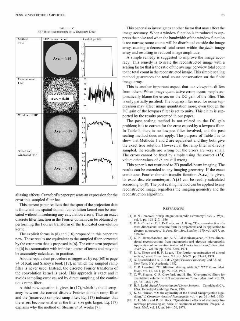
This section uses a computer simulated phantom to demon-strate the effectiveness of the post scalingmethod to improve thereconstruction accuracy. The parallel-beam imaging geometryis used to analytically generate projections with Poisson noiseadded. The number of views is 120 over 360 . There are 128detector bins on the detector. The images are reconstructed in a

array with , where is the length of thediscrete convolution kernel used to evaluate the discrete filter asdefined in (5). The results are shown in Table IV. These imaging

parameters are typical values in our Siemens SPECT system,where the image resolution is approximately 1 cm which is a lotlarger than the pixel size. The purpose of Table IV is to com-pare the average image value in a large uniform region, and theimage resolution is not considered.The “Conventional FBP” method uses Method 4 defined in

Part A of this section, without any window functions. The “Win-dowed FBP” methods uses the window function developed in[11], and is given as

(18)

where , , andprojection value of the current ray-sum. This window functionmodels the Poisson noise in the projections. This window func-tion changes from ray to ray. Whenis defined as 1.When the filter is spatially variant, the Fourier domain fil-

tering is carried out as follows. The spatially variant filter isquantized into 11 spatially invariant filters and apply these 11filters to the projections, one filter at a time. Thus, 11 versions ofthe filtered projections are obtained. According to noise level ofeach ray, a filtered ray is selected from one of these 11 versions.At the end, only one backprojection is required to complete theFBP reconstruction.The scaling factor in the “Scaled andwindowed FBP”method

is calculated according to (11). Due to noise, the value of the“sum of measured projections at one view” is chosen as the sumof all measurements divided by the number of views. The valueof the “sum of FBP reconstruction” is sum of thereconstruction array with all negative image values set to zero.All images in Table IV are displaying the same image value

range of [ ], where -0.1 corresponds to black and 0.5corresponds to white. The display gray scale is linear. The av-erage value within the disc is labeled in the center of the image.One last observation is that Method 4 gives large errors

in Table III with , while the errors of Method 4 inTable IV are invisible for if no lowpass filter isapplied. This observation verifies that the DC gain and low-fre-quency gain errors are visible only for a small . The lowpassfilter has a more significant effect on image quantitation for alarge .

IV. DISCUSSION AND CONCLUSIONS

This paper re-visits the well-known ramp filter, which is thedriving engine in the FBP algorithm. This paper gives an exactformula (16) for the discrete ramp filter and also calculates theapproximation error if one chooses to directly sample the con-tinuous ramp filter. This common practice is then justified. Animmediate result is that in order to reduce the errors, all one hasto do is to pad more zeros (i.e., to increase ) to the projectiondata before transforming them into the Fourier domain.Now the proposed approach is compared with that presented

in [6]. The main difference is as follows. In Crawford’s paper[6], the discrete Fourier domain filter is obtained by samplingthe continuous ramp filter. Since the corresponding spatial-do-main convolution kernel has an infinite span, discrete samplingin the Fourier domain with any sampling interval will cause

ZENG: REVISIT OF THE RAMP FILTER 135

TABLE IVFBP RECONSTRUCTION OF A UNIFORM DISC

aliasing effects. Crawford’s paper presents an expression for theerror this sampled filter has.This current paper realizes that the span of the projection data

is finite and the spatial-domain convolution kernel can be trun-cated without introducing any calculation errors. Thus an exactdiscrete filter function in the Fourier domain can be obtained byperforming the Fourier transform of the truncated convolutionkernel.The explicit forms in (8) and (16) proposed in this paper are

new. These results are equivalent to the sampled filter correctedby the error term that is proposed in [6]. The error term proposedin [6] is a summation with infinite number of terms and may notbe accurately calculated in practice.Another equivalent procedure is suggested by eq. (68) in page

74 of Kak and Slaney’s book [17], in which the sampled rampfilter is never used. Instead, the discrete Fourier transform ofthe convolution kernel is used. This approach is exact and itavoids sampling error caused by direct sampling of the contin-uous ramp filter.A third new equation is given in (17), which is the discrep-

ancy between the correct discrete Fourier domain ramp filterand the (incorrect) sampled ramp filter. Eq. (17) indicates thatthe errors become smaller as the filter size gets larger. Eq. (17)explains why the method of Stearns et al. works [7].

This paper also investigates another factor that may affect theimage accuracy. When a window function is introduced to sup-press the noise and when the bandwidth of the window functionis too narrow, some counts will be distributed outside the imagearray, causing a decreased total count within the finite imagearray and resulting in reduced image amplitude.A simple remedy is suggested to improve the image accu-

racy. This remedy is to scale the reconstructed image with ascaling factor that is the ratio of the average per-view total countto the total count in the reconstructed image. This simple scalingmethod guarantees the total count conservation on the finiteimage array.This is another important aspect that our viewpoint differs

from others. When image quantitative errors occur, people au-tomatically blame the errors on the DC gain of the filter. Thisis only partially justified. The lowpass filter used for noise sup-pression may affect image quantitation more, even though theDC gain of the lowpass filter is set to unity. This claim is sup-ported by the results presented in our paper.The post scaling method is not related to the DC gain

problem; it is to correct for the error caused by a lowpass filter.In Table I, there is no lowpass filter involved, and the postscaling method does not apply. The purpose of Table I is toshow that Methods 1 and 2 are equivalent and they both givethe exact true solution. However, if the ramp filter is directlysampled, the results are wrong but the errors are very small.The errors cannot be fixed by simply using the correctvalue; other values of are still wrong.This paper is not restricted to 2D parallel-beam imaging. The

results can be extended to any imaging geometry. If the exactcontinuous Fourier domain transfer function is given,its exact discrete counterpart can be readily calculatedaccording to (8). The post scaling method can be applied to anyreconstructed image, regardless the imaging geometry and thereconstruction algorithm.

REFERENCES

[1] R. N. Bracewell, “Strip integration in radio astronomy,” Aust. J. Phys.,vol. 9, pp. 198–217, 1956.

[2] R. A. Crowther, D. J. DeRosier, and A. Klug, “The reconstruction of athree-dimensional structure form its projections and its application toelectron microscopy,” in Proc. Roy. Soc. London, 1970, vol. A317, pp.319–340.

[3] G. N. Ramachandran and A. V. Lakshminarayanan, “Three-dimen-sional reconstructions from radiographs and electron micrographs:Application of convolution instead of Fourier transforms,” Proc. Nat.Acad. Sci., vol. 68, pp. 2236–2240, 1971.

[4] L. A. Shepp and B. F. Logan, “The fourier reconstruction of a headsection,” IEEE Trans. Nucl. Sci., vol. NS-21, pp. 21–43, 1974.

[5] A. Rosenfeld and A. C. Kak, Digital Picture Processing, 2nd Ed. ed.New York, NY: Academic, 1982.

[6] C. R. Crawford, “CT filtration aliasing artifacts,” IEEE Trans. Med.Imag., vol. 10, no. 1, pp. 99–102, 1991.

[7] C. W. Stearns, C. R. Crawford, and H. Hu, “Oversampled filters forquantitative volumetric PET reconstruction,” Phys. Med. Biol., vol. 39,pp. 381–387, 1994.

[8] B. P. Lathi, Signal Processing and Linear Systems. Carmichael, CA,USA: Berkeley-Cambridge Press, 1998.

[9] K. M. Hanson, “On the optimality of the filtered backprojection algo-rithm,” J. Computer Assisted Tomography, vol. 4, pp. 361–363, 1980.

[10] C. E. Metz and R. N. Beck, “Quantitative effects of stationary lin-earimage processing on noise of resolution of structure images,” J.Nucl. Med., vol. 15, pp. 164–170, 1974.

136 IEEE TRANSACTIONS ON NUCLEAR SCIENCE, VOL. 62, NO. 1, FEBRUARY 2015

[11] D. A. Chesler and S. J. Riederer, “Ripple suppression during recon-struction in transverse tomography,” Phys. Med. Biol., vol. 20, pp.632–636, 1975.

[12] R. W. Hamming, Digital Filters. Englewood Cliffs, NJ, USA: Pren-tice Hall, 1977.

[13] S. Butterworth, “On the theory of filter amplifiers,” Experimental Wire-less and the Wireless Engineer, vol. 7, pp. 536–541, 1930.

[14] G. L. Zeng and A. Zamyatin, “A filtered backprojection algorithmwith ray-by-ray noise weighting,” Med. Phys., vol. 40, 031113, Feb.28, 2013 [Online]. Available: http://dx.doi.org/10.1118/1.4790696, 7pages

[15] L. A. Shepp and Y. Vardi, “Maximum likelihood reconstruction foremission tomography,” IEEE Trans. Med. Imag., vol. 1, no. 2, pp.113–122, Oct. 1982.

[16] Y. Vardi, L. A. Shepp, and L. Kaufman, “A statistical model forpositron emission tomography,” J. Amer. Stat. Assoc., vol. 80, pp.8–20, 1985.

[17] A. C. Kak and M. Slaney, Principles of Computerized TomographicImaging. Philadelphia, PA, USA: Society of Industrial and AppliedMathematics, 2001.