ieee transactions on medical imaging, vol. 32, no. 2...

IEEE TRANSACTIONS ON MEDICAL IMAGING, VOL. 32, NO. 2, FEBRUARY 2013 141

Noise Properties of Motion-CompensatedTomographic Image Reconstruction Methods

Se Young Chun*, Member, IEEE, and Jeffrey A. Fessler, Fellow, IEEE

Abstract—Motion-compensated image reconstruction (MCIR)methods incorporate motion models to improve image quality inthe presence of motion. MCIR methods differ in terms of howthey use motion information and they have been well studiedseparately. However, there have been less theoretical comparisionsof different MCIR methods. This paper compares the theoret-ical noise properties of three popular MCIR methods assumingknown nonrigid motion. We show the relationship among threeMCIR methods—motion-compensated temporal regularization(MTR), the parametric motion model (PMM), and post-recon-struction motion correction (PMC)—for penalized weightedleast square cases. These analyses show that PMM and MTRare matrix-weighted sums of all registered image frames, whilePMC is a scalar-weighted sum. We further investigate the noiseproperties of MCIR methods with Poisson models and quadraticregularizers by deriving accurate and fast variance predictionformulas using an “analytical approach.” These theoretical noiseanalyses show that the variances of PMM and MTR are lowerthan or comparable to the variance of PMC due to the statisticalweighting. These analyses also facilitate comparisons of the noiseproperties of different MCIR methods, including the effectsof different quadratic regularizers, the influence of the motionthrough its Jacobian determinant, and the effect of assuming thattotal activity is preserved. Two-dimensional positron emissiontomography simulations demonstrate the theoretical results.

Index Terms—Motion-compensated image reconstruction, noiseproperties, nonrigid motion, quadratic regularization.

I. INTRODUCTION

M OTION-COMPENSATED image reconstruction(MCIR) methods have been actively studied for var-

ious imaging modalities. MCIR methods can provide highsignal-to-noise ratio (SNR) images (or low radiation doseimages) and reduce motion artifacts [1]–[14]. Gating methodsimplicitly use motion information (i.e., no explicit motionestimation required) for motion correction, but yield low SNRimages due to insufficient measurements (or require longeracquisition to collect enough measurements) [15], [16]. Incontrast, MCIR methods use explicit motion information (i.e.,

Manuscript received April 17, 2012; revised June 20, 2012; accepted June26, 2012. Date of publication June 29, 2012; date of current version January 30,2013. This work was supported in part by the National Institutes of Health/Na-tional Cancer Institute (NIH/NCI) under Grant 1P01 CA87634. Asterisk indi-cates corresponding author.*S. Y. Chun is with the Department of Electrical Engineering and Computer

Science and Radiology, University of Michigan, Ann Arbor, MI 48109 USA(e-mail: [email protected]).J. A. Fessler is with the Department of Electrical Engineering and Com-

puter Science, University of Michigan, Ann Arbor, MI 48109 USA. (e-mail:[email protected]).Color versions of one or more of the figures in this paper are available online

at http://ieeexplore.ieee.org.Digital Object Identifier 10.1109/TMI.2012.2206604

motion estimation obtained jointly or separately) to correctfor motion artifacts and to produce high SNR images with allcollected data.This paper analyzes three popular MCIR methods that

differ in their way of incorporating motion information:post-reconstruction motion correction (PMC) [1]–[3], mo-tion-compensated temporal regularization (MTR) [4], [5], andthe parametric motion model (PMM) [6]–[14]. Each MCIRmethod has been well studied separately, but there has been lesstheoretical research on comparing different MCIR methods.There are some empirical comparisons between PMC andPMM [17], [18], and between MTR and PMM [19]. Asma etal. compared PMC and PMM theoretically in terms of theirmean and covariance by using a discrete Fourier transform(DFT) based approximation [20]. However, the analytical com-parison was limited to the unregularized case and the empiricalcomparison was performed for the regularized case.Theoretical noise analyses of MCIR methods can be useful

for regularizer design and for performance comparisons. Noiseprediction methods include matrix-based approaches [21],DFT methods [22], and an “analytical approach” that is muchfaster [23]. We extend this analytical approach to MCIR, andinvestigate the noise properties of PMC, PMM, and MTR withquadratic regularizers theoretically, assuming known nonrigidmotion. This assumption is applicable to some multi-modalmedical imaging systems such as positron emission tomog-raphy-computerized tomography (PET-CT) [7], [8], [10] andPET-MR [14]. These analyses provide fast variance predictionfor MCIR methods and may also provide some insight intounknown motion cases. These noise analyses not only facilitatetheoretical comparisons of the performance of different MCIRmethods, but also help one understand the influence of themotion (through its Jacobian determinant) and the effect ofassuming that the total activity is preserved.This paper is organized as follows. Section II reviews the

basic models and the estimators of the MCIR methods [24]:PMC, PMM, andMTR. Section III shows the similarity and dif-ference between three MCIR estimators in penalized weightedleast square (PWLS) cases. It shows that MTR and PMM are es-sentially the Fisher information-based matrix-weighted sum ofall registered image frames, while PMC is the scalar-weightedsum. Section IV derives fast variance prediction formulas forPMC and PMM with Poisson likelihoods and general quadraticregularizers. Section V compares the theoretical noise proper-ties of MCIRmethods. Section VI illustrates the theories by 2-DPET simulations with digital phantoms for given affine and non-rigid motions.

0278-0062/$31.00 © 2012 IEEE

142 IEEE TRANSACTIONS ON MEDICAL IMAGING, VOL. 32, NO. 2, FEBRUARY 2013

II. MCIR MODELS AND METHODS

This section reviews MCIR models that were also describedin [24] and derives the PWLS estimator for each model.Although we focus on PWLS for simplicity, the general con-clusions are also applicable to penalized-likelihood estimationbased on Poisson models [25]. We consider three MCIRmethods: PMC [1]–[3], PMM [6]–[12], [26], [27], and MTR[4], [5], [19], [28]. We treat the nonrigid motion information aspredetermined (known) and focus on how the motion modelsaffect noise propagation from the measurements into the recon-structed image. In practice, errors in the motion models lead tofurther variability in the image.

A. Review of Basic MCIR Models

1) Measurement Model: MCIR methods are needed whenthe time-varying object has non-negligible motionduring an acquisition interval where denotes spatialcoordinate and denotes time. Often one can use gating ortemporal binning to group the measurements into sets, called“frames” here. Let denote the vector of measurements asso-ciated with the th frame. We assume the time varying object

is approximately motionless during the acquisition ofeach . Let denote the time associated with the th frame,and let denote a spatialdiscretization of the object where denotes the centerof the th voxel for , and denotes the numberof voxels. We assume that the measurements are related to theobject linearly as follows:

(1)

where denotes the system model for the th frame,denotes noise, and is the number of gates or frames.We allowthe system model to possibly differ for each frame.2) Warp Model: For a given spatial transformation

, define a warp operator as follows:

(2)

where the total activity is preserved when . We discretizethe warp to define a matrix relating the imageto the image as follows:

(3)

For applications with periodic motion, we can additionally de-fine and . The matrixcan be implemented with any interpolation method; we used aB-spline based image warp [29]. Let denote the de-terminant of the Jacobian matrix of a transform for awarp . Throughout we assume the warps (or equiv-alently or ) are known. We also assume that invert-ibility, symmetry, and transitivity properties hold for [24].

B. Single Gated Reconstruction (SGR)

Often one can reconstruct each image from the corre-sponding measurement based on the model (1) and someprior knowledge (e.g., a smoothness prior). A single gated(frame) reconstruction (SGR) can be obtained as follows:

(4)

where , is a negative likelihood functionderived from (1), is a spatial regularizer, and is a spatialregularization parameter.For the PWLS case, i.e.,

where is a weight matrix that usuallyapproximates the inverse of the covariance of , one canobtain a closed form estimator as follows:

(5)

where the Fisher information matrix for the th frame is“ ” denotes matrix transpose, and is the Hes-

sian matrix of a quadratic regularizer .

C. Post-Reconstruction Motion Correction (PMC)

Once the frames are reconstructed individuallyfrom (4), one can improve SNR by averaging all reconstructedimages. Using the motion information to map each imageto a single image’s coordinates can reduce motion artifacts.Without loss of generality, we chose as our reference image.Using (3) and (4), a natural definition for the (scalar-weighted)PMC estimator is the following motion-compensated average:

(6)

where . One choice is for all(unweighted PMC). Another option iswhere is the acquisition time (or the number of counts) forthe th frame (scalar-weighted PMC). For the PWLS case,there is an explicit form for using (3), (5), and (6)

(7)

where and are es-sentially Hessian matrices for the th frame in the coordinatesof the first (reference) frame.

D. Parametric Motion Model (PMM)

Without loss of generality, we assume that is our referenceimage frame for the PMM approach. Combining the measure-ment model (1) with the warp (3) yields a new measurementmodel that depends only on the image instead of the all im-ages (i.e., parameterizing all images with )

CHUN AND FESSLER: NOISE PROPERTIES OF MOTION-COMPENSATED TOMOGRAPHIC IMAGE RECONSTRUCTION METHODS 143

Stacking up these models yields the overall model

(8)

where the components are each stacked accordingly

and

(9)

The PMM estimator for the measurement model (8) with a spa-tial regularizer is

(10)

where is a negative likelihood function and is a spatialregularizer.For the PWLS data fidelity function

where is a diag-onal matrix, the PMM estimator is

(11)

where is a block-di-agonal matrix, and is the Hessian matrix of a quadraticregularizer . Since we canrewrite the PMM estimator in (11) as

(12)

E. Motion-Compensated Temporal Regularization (MTR)

The MTR method incorporates the motion information thatmatches two adjacent images into a temporal regularizationterm [4], [5]

(13)

for . This penalty is added to the cost functionin (4) for all to define the MTR cost function.Equation (4) for all and (13) can be represented in a simpler

vector-matrix notation. First, stack up (1) for all as follows:

(14)

where and , are defined in (9). Then,the MTR estimator based on (13) and (14), and a spatial regu-larizer is

(15)

where is a negative likelihood function from the noise modelof (14), is a spatial regularizer, is a temporal regularizationparameter, and the temporal differencing matrix is

. . .. . . (16)

We may also modify for periodic (or pseudo-periodic)image sequences by adding a row corresponding to the term

. Note that unlike the PMMmethod that estimatesone frame , MTR estimates all image frames . The MTRestimate of (reference image) is

(17)

For the PWLS case, the solution to (15) is

(18)

where and .

III. RELATIONSHIP BETWEEN MCIR ESTIMATORS

In this section, we investigate the relationship among PWLSMCIR estimators in (5), (7), (12), and (18). Considering PWLSestimators helps show the similarity and differences amongMCIR methods more clearly than estimators for Poissonlikelihoods. Although the observations in this section focuson PWLS estimators, similar results can be obtained for themean and variance of MCIR estimators with Poisson likelihoodmodels [25]. The next section analyzes the variance of theseMCIR methods.

A. Properties of MTR Estimator for and

The temporal regularization term (13) in (15) will increasethe correlation between the estimators and for asis increased. Even though (18) provides the exact relationshipbetween the PWLS MTR estimator and , this form itself maynot be informative in terms of comparing it with other MCIRmethods. So, we investigate the limiting behavior of the PWLSMTR estimator as and as . This provides insightsfor comparisons with PMM and PMC.It is straightforward to determine the limit of in (18) as

because

(19)

where is a block-diagonal matrix, i.e.,Therefore, as , the PWLS

MTR estimator approaches

(20)

where are defined in (5). Thus, by (17), as. In other words, as , the PWLS MTR estimator for

each frame approaches the PWLS SGR estimator (5).As , has more interesting limiting behavior. The

following theorem is proven in Appendix A.


Theorem 1: As , the MTR estimator becomes

(21)

where , is defined in (9),

, and .

B. Equivalence of MTR and PMM Estimators

Equation (21) in Theorem 1 and (12) show that the PWLSestimators of PMM and MTR are remarkably similar.In particular, if we choose a PMM regularizer with

(22)

then the analysis leading to (21) with (17) shows that

(23)

In other words, as . Therefore, assumingsome mild conditions on motion and spatial regularizers, thePWLS estimators of PMM and MTR with sufficiently largewill be approximately the same, and thus so will the mean andcovariance. For the Poisson likelihood, one can show that themean and covariance of the MTR estimator will approach themean and covariance of the PMM estimator as increases. Wewill show the covariance case for the Poisson likelihood in thenext section. The mean case with the Poisson likelihood can beshown by consulting [24] and using Appendix A.

C. Difference Between PMC and PMM Estimators

Using (5), (7), and (22), we rewrite the PWLS PMMestimator(12) as follows:

(24)

where the weighting matrices are given by

(25)

Comparing the PWLS PMM estimator (24) and the PWLSPMC estimator (6), we see that the PWLS PMC estimator is ascalar-weighted average of the motion corrected PWLS SGRestimators of all frames whereas the PWLS PMM estimator isa matrix-weighted average of the motion corrected PWLS es-timators. The PWLS MTR estimator (with proper motion andregularizers) approaches the same matrix-weighted average ofthe motion corrected estimators (24) as .

The weights in (25) are calculated using the Fisher in-formation matrices . This implies that the PWLS PMM es-timator (and the PWLS MTR estimator with ) automat-ically assigns different weights to the estimate dependingon factors such as noise (Fisher information matrix ) andmotion . For the Poisson likelihood case, the next sectionshows the benefit of this matrix-weighted average (24) by inves-tigating the noise properties of MCIR methods using an “ana-lytical approach” extended from [24] and [23].

IV. NOISE PROPERTIES OF MCIR

This section analyzes the noise properties of different MCIRmethods. The analysis applies both to PWLS estimators andto maximum a posteriori (MAP) estimators based on Poissonlikelihoods. Since the analysis is based on a first-order approx-imation of the gradient of the likelihood, the accuracy of theanalysis for Poisson likelihoods will decrease as the number ofcounts per frame decreases as shown in [25]. For simplicity, wefocus on 2-D PET with a few assumptions. We consider an idealtomography system, i.e., we ignore detector blur. We also as-sume that for all . The (unitless) elements ofdescribe the probability that an emission from the th pixel

is recorded by the th detector in the absence of attenuation orscatter and for an ideal detector. The th element of the diagonalmatrix has units of time and includes the detector efficiency,the patient-dependent attenuation along the th ray, and the ac-quisition time for the th frame.We assume known attenuation map (i.e., is given), which

is the usual assumption for PET-CT [30] or PET-MR [31]. Westill allow the warp to differ for each . We assume thatthe given nonrigid motion is locally affine [24]. We also as-sume that the measurements for all are independent, i.e.,

for all .We use an “analytical approach” to derive approximate vari-

ances for SGR and MCIR methods. This appproach providesfast variance prediction methods [23] compared to the DFT-based variance approximations or numerical simulations.

A. Single Gated Reconstruction (SGR)

If in (4) is a negative Poisson log-likelihood function (i.e.,), then one can approximate the

covariance of the SGR estimator of (4) by [25]

(26)

where , isa diagonal matrix, is the mean of , the Hessian of theregularizer is , and .To study (26) using the “analytical approach” of [23], we

focus on a first-order difference quadratic regularizer

(27)

where denotes 2-D convolution, is a non-negative regu-larization weight (e.g., regularization designs for uniform and/orisotropic spatial resolution [24], [32]), denotes the 2-D


array corresponding to the lexicographically ordered vector ,is the lexicographic index of the pixel at 2-D coordinates ,and

(28)

where denote the spatial offsets of the th pixel’s neigh-bors and denotes the 2-D Kronecker impulse. We usedthe usual 8-pixel 2-D neighborhood with and

.For a polar coordinate in the frequency domain, we can

represent the variance of (26) at the th voxel in an analyticalform as follows [23]:

(29)

where , is the pixel spatial sampling distance,and the local power spectrum at the th pixel, whichis the Fourier transform of the th column of the covariance in(26) (see also [33, p. 220]), is

(30)

where the angular component of the local frequency responseof the regularizer (27) is

(31)

and . For a standard quadratic regularizer,where is a constant. The analytical forms of and

at the th voxel are and (see [23]and [32]) where

(32)

is the set of rays at the angle , ,, , is a de-

tector sampling interval, and is an angular sam-pling interval. For fast computation, one can approxi-mate where

. One can further simplify the localvariance in (29) by calculating the intergral (29)with respect to as follows [23]:

(33)

where . The variance of the SGRestimator for the Poisson likelihood depends on the measure-ment statistics , the sampling distances , , , and theregularization parameter . One can also obtain the local au-tocovariance of the SGR estimator at the th pixel by taking

an inverse Fourier transform (FT) of the local power spectrumin (30).

B. Post-Reconstruction Motion Correction (PMC)

Assuming that the measurements for each frame are sta-tistically independent and the reconstruction algorithm uses thePoisson likelihood, the covariance of the PMC estimator (6) isapproximately

(34)

We can derive the analytical forms of and [the quadraticregularizer (27)] in the frequency domain as follows (see [24,Appendix B]):

(35)

(36)

where is the closest pixel to and. Therefore, by using analyt-

ical forms, we approximate the variance of at the thvoxel

(37)

where the local power spectrum, , at the th pixel isgiven by

where the following factors arise from the Fisher informationmatrix and the Hessian of the regularizer , respectively,due to motion compensation

(38)

For rigid motion, whereas for nonrigidmotion such as (isotropic or anisotropic) scaling, and

usually differ from 1. By integrating, we simplify thelocal variance in (37) further as follows:

(39)


Note that the variance of the PMC estimator depends on the mo-tion through and terms. One can also obtain thelocal autocovariance of the PMC estimator by taking an inverseFT of .

C. Parametric Motion Model

For the PMM estimator (10) with the Poisson likelihood, thecovariance of the PMM estimator, , can be approx-imated using the matrix-based methods of [25] as

(40)Using the analytical forms in (35) and (36), the variance of thePMM estimator at the th pixel is approximately

(41)

where the local power spectrum, , at the th pixelfor (40) is defined as follows:

where . Integratingover simplifies the local variance

in (41) to

(42)

Like the PMC case, the noise depends on the given motion. Thelocal covariance of the PMM estimator can be approximatedwith an inverse FT of .The covariance of the PMM estimator with the regularizer

(22) will be approximately

(43)

and with the same procedure as above, the variance of the PMMestimator at the th pixel for (43) is approximately

(44)

One can evaluate (33), (39), (42), and (44) using a simple backprojection (i.e., approximate integral by sum over projectionangle ) to predict variance for every image pixel.

D. Motion-Compensated Temporal Regularization

From (15) with the Poisson likelihood, the covariance matrixof the MTR estimator is approximately

(45)

where . Section III showed that the PWLSMTR estimator converges to the PWLS SGR and PMM estima-tors as and , respectively. For the estimators withthe Poisson likelihood, one can show that the covariance of theMTR estimator (45) “approximately” converges to the covari-ance of the SGR estimator and the PMM estimator asand , respectively, using (64) in Appendix A. Therefore,the local variance of the MTR estimator at the th pixel will ap-proach the SGR result (33) approximately as and willapproach the PMM result (44) approximately as .Obtaining an analytical form for the variance of MTR with

any seems challenging due to the complicated structure ofmatrix. However, from (45) one can show that the co-

variance of the MTR decreases as increases. We can also intu-itively expect that high value will increase the correlation be-tween estimated image frames, which will reduce the varianceof MTR. We evaluate this intuition empirically in Section VI.

V. PERFORMANCE COMPARISONS IN MCIR

This section presents theoretical comparisons of the noiseproperties of SGR and MCIR methods with the Poisson like-lihood.

A. Comparing Noise Properties Between PMC and PMM

As discussed in Section III-C, the PMC estimator is ascalar-weighted average of the motion corrected estimators ofall frames, whereas the PMM estimator is a matrix-weightedaverage using the weight in (25). This difference led to thedifferent variances of the PMC estimator (39) and of PMM(44) (and the variance of MTR for ). By matching thespatial resolutions of PMM and PMC using the regularizer (22)for PMM (see [24]), we can also compare the variance of PMCand PMM theoretically.For , one can show that

(46)

using the Cauchy–Schwarz inequality [20] and .If we set

then (39), (44), and (46) show that

(47)

for the regularized PMC and PMM. Equality holds when allare the same for all . This inequality is consistent with theempirical observations in [20]. Therefore, PMM (andMTRwithsufficiently large ) is preferable over PMC in terms of noisevariance.

B. Comparing Noise Properties of SGR for Three Regularizers

Because of the interactions between the likelihood and regu-larizer, spatial resolution will be anisotropic and nonuniform ifone uses a standard regularizer [21], i.e., in (30),


which we call SGR-S. There has been some research on reg-ularizers that provide approximately uniform and/or isotropicspatial resolution [21], [32], [34]. This section analyzes the ef-fect of such regularizers on the noise properties of SGR.The certainty-based quadratic regularizer proposed in [21]

can provide approximately uniform (but still anisotropic) spa-tial resolution. In this case, in (27) is designed to approxi-mately satisfy

(48)

and we call the estimation SGR-C. Alternatively, one can designto approximately satisfy

(49)

so that the spatial resolution will be approximately uniformand isotropic [32], [35], which we call SGR-P. From (33), onecan show the relationship between the variances of SGR-S andSGR-C as follows:

(50)

The same relationship holds between SGR-S and SGR-P. Thevariance of SGR-S can be larger or smaller than the variance ofSGR-C and SGR-P for each location ( th pixel).There is a more interesting relationship between the variances

of SGR-C and SGR-P. In both (48) and (49),[21], [32], and substituting this further approximation

into (33) yields the following simplified variance approxima-tion:

(51)

This approximation becomes increasingly accurate asand/or increase. In our simulations, using (49) in (51) signifi-cantly reduced the accuracy of (51) because small differencesin (49) became large differences in (51) due to their reciprocalrelationship. Using (48) and (49) to achieve approximately uni-form and/or isotropic spatial resolution will increase the effectof the measurement statistics on the estimator variance(51) compared to (33). This tendency was empirically observedin [21]. Using the Cauchy–Schwarz inequality, one can showthat the variance approximation in (51) satisfies

(52)

This inequality is verified empirically in Section VI-B. Evi-dently, imposing more properties on the spatial resolution suchas isotropy requires sacrificing the noise performance, whichshows the spatial resolution-noise trade-off.

C. Comparing Noise Properties Between SGR and MCIR

If there is no motion between image frames andfor all , then (33), (39), and (44) yield

, as expected since PMC andPMM used times more counts than SGR. The MTR variance

with very high also yields approximately thesame variance as PMM and PMC in this case.However, this relationship between MCIR and SGR

variances may not hold exactly when there is motion betweenimage frames. For example, if there is locally isotropic scalingmotion between frames as follows:

(53)

where , then and in(38). For PMC, if we design the regularizer to achieve isotropicresolution by using

(54)

and if and/or are relatively large, then the variance of thePMC estimator at the th pixel in (39) approximately reduces to

(55)

Comparing with (51), the variance of PMC (55) will be approx-imately times the variance of SGR for . Thevariance of PMM (44) will have a similar relationship with thevariance of SGR. If the total activity is preserved (i.e., ),then local expansion will increase the variance andlocal shrinkage will decrease the variance. Intuitively,if the same amount of total activity produces the same numberof Poisson counts, the expanded area that contains the same totalactivity will have larger image area to estimate, i.e., effectivelymore parameters. Thus, the expanded area will lead to higher es-timator variance. For regularizers other than (54), the varianceof PMC will also be affected by motion through and

terms.

D. Total Activity Preserving Condition for MCIR

The total activity preserving condition (2) is important for ac-curate motion modeling and it also affects the spatial resolution[24] and noise properties of MCIR. Using the example in Sec-tion V-C, we analyze the influence of motion on the noise, fo-cusing on PMC and PMM. (MTR with sufficiently large willhave approximately the same noise properties as PMM.)If one uses standard quadratic regularizers for PMC and

PMM [e.g., and in (31)],then the variance of the PMC estimator in (39) reduces to

(56)

since and when (53) holds. Thevariance of the PMM estimator in (42) reduces to

(57)

When (e.g., rigid motion), the variance is not affectedby motion. However, when , the variance of PMC will


be always affected by motion, whether the total activity is pre-served or not, due to the and terms in (56). However,when and/or are relatively large, the variance of PMMmay be less affected by motion when than whensince (57) only contains , which is relatively closer to 1 thanor . Since the regularizer in PMM does not involve the

motion warp, there is no term in the variance (42) ofPMM. Thus, when we use the total activity preserving condi-tion with the standard regularizers, the variance of PMMmay be less affected by motion than the variance of PMC.When one designs the spatial regularizers [i.e., determinein (27)] to achieve approximately uniform and/or isotropic

spatial resolution for the MCIR methods [24], as shown inSection V-C, the variances of PMC and PMM will be affectedby motion with the factor of . Thus, the variance of PMCand PMM will be less affected by motion when thanwhen . Note that the analyses above assumed that bothmeasurement model and reconstruction model follow the samecondition. One could generalize these analyses to consider theeffects of motion model mismatch.

VI. SIMULATION RESULTS

The analyses in this paper apply to nonrigid motions that areapproximately locally affine [24]. We performed PET simula-tions with two digital phantoms: one is a simple phantom withglobal affine motion between frames and the other is the XCATphantom [36] with nonaffine nonrigid motion that we modeledusing B-splines [37].

A. Simulation Setting

Two digital phantoms were used, each with four frames of160 160 pixels with 3.4 mm pixel width. Sinogramswere gen-erated using a PET scanner geometry with 400 detector samples,1.9 mm spacing, 220 angular views, and 1.9 mm strip width. Weused 300 K, 500 K, 200 K, 200 K mean true coincidences foreach frame (1.2M total) with 10% random coincidences. Simpleuniform attenuation maps were used for the first simulation andno attenuation was used for the second.We investigated SGR, PMC, and PMM by comparing an-

alytical standard deviation (SD) with empirical SD from 500Poisson noise realizations. We used spatial regularizers (withregularization parameter ) that provide approximatelyuniform (SGR-C, PMC-C, PMM-C) and uniform/isotropic(SGR-P, PMC-P, PMM-P) spatial resolutions, respectively[20], [21], [24], [32]. We also studied the noise properties ofMTR empirically with various values. The spatial resolutionsof SGR, PMC, PMM, and MTR were all matched to eachother using the regularization designs in [24]. All images werereconstructed using a L-BFGS-B (quasi-Newton) algorithmwith non-negativity constraints [38], [39].

B. Simple Phantom With Affine Motion

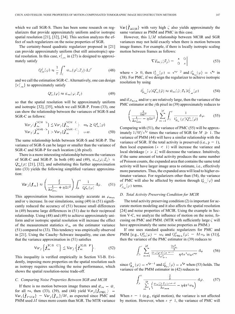
We used a simple digital phantom with known affine motion(anisotropic scaling between frame 1 and 2, rotation betweenframe 2 and 3, and translation between frame 3 and 4) as shownin Fig. 1. The total activity is preserved between frames.Fig. 2 displays profiles through the variance image and shows

that our analytical equation for SGR in (33) [and (51)] provides

Fig. 1. Four true images with anisotropic scaling, rotation, and translation.Total activity is preserved.

Fig. 2. Analytical SD of SGR (A-SGR-P, A-SGR-C) matches well with em-pirical SD of SGR (E-SGR-P, E-SGR-C), respectively. SD of SGR-P (with reg-ularizer that approximately uniform and isotropic spatial resolution) is higherthan SD of SGR-C (with regularizer that approximately uniform spatial resolu-tion), which is consistent with theoretical comparison.

accurate noise predictions. (The location of the profile is indi-cated in Fig. 1 as a horizontal line). The analytical SD of SGRwith quadratic regularizers (A-SGR-C and A-SGR-P) matcheswell with the empirical SD of SGR from 500 noise realizations(E-SGR-C and E-SGR-P). Fig. 2 also shows that the varianceof SGR-C is lower than the variance of SGR-P as shown in (52)(in this case, was fairly large). This analytical and empiricalagreement of SGR does not hold well near the boundary of andoutside the object because of the non-negativity constraint andbecause the “locally shift invariant” approximation is less accu-rate there. We observed similar results for a constant quadraticregularizer (not shown).Fig. 3 shows that our analytical variance prediction for PMC

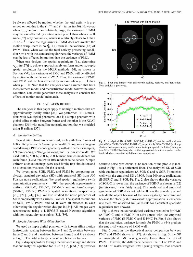
(A-PMC-C and A-PMC-P) in (39) agrees with the empiricalvariance of PMC (E-PMC-C and E-PMC-P). Fig. 4 also showsthat the analytical variance formula for PMM in (44) predictsthe empirical variance of PMM well.Fig. 5 confirms the theoretical noise comparison between

PMC and PMM shown in (47). As shown in Fig. 5, the SDof unweighted PMC was generally lower than the SD ofPMM. However, the difference between the SD of PMM andthe SD of scalar-weighted PMC (using weights that account


Fig. 3. Analytical SD of PMC (A-PMC-P, A-PMC-C) matches well with em-pirical SD of PMC (E-PMC-P, E-PMC-C), respectively.

Fig. 4. Analytical SD of PMM (A-PMM-P, A-PMM-C) matches well with em-pirical SD of PMM (E-PMM-P, E-PMM-C), respectively.

Fig. 5. If the spatial resolutions are matched, the SD of PMC is higher than orcomparable to the SD of PMM, depending on the choice of weights .

for the number of counts per frame) was very small. Usingthe spatial regularizer for PMM as proposed in (22) thatmatches to PMC, the full-width at half-maximum (FWHM)of PMC pixels was slightly larger than theFWHM of PMM pixels . Our target FWHM was

. This small discrepancy was because ouranalysis assumed perfect interpolations for warps, whereasthe actual interpolations induce slight blurring. For PMC, thewarp is applied after the reconstruction, thus the FWHM wasslightly larger than the target FWHM. We observed that the

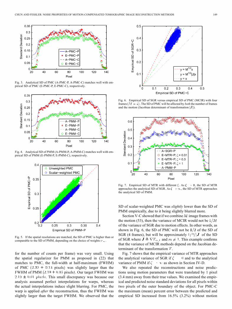
Fig. 6. Empirical SD of SGR versus empirical SD of PMC (MCIR) with fourframes . The SD of PMCwill be affected by both the number of framesand the motion (Jacobian determinant of transformation ).

Fig. 7. Empirical SD of MTR with different . As , the SD of MTRapproaches the analytical SD of SGR. As , the SD of MTR approachesthe analytical SD of PMM.

SD of scalar-weighted PMC was slightly lower than the SD ofPMM empirically, due to it being slightly blurred more.Section V-C showed that if we combine image frameswith

the motion (53), then the variance of MCIR would not beof the variance of SGR due to motion effects. In other words, asshown in Fig. 6, the SD of PMC will not be of the SD ofSGR (4 frames), but will be approximately of the SDof SGR where and . This example confirmsthat the variance of MCIR methods depend on the Jacobian de-terminant of the transformation .Fig. 7 shows that the empirical variance of MTR approaches

the analytical variance of SGR if and to the analyticalvariance of PMM if as shown in Section IV-D.We also repeated the reconstructions and noise predic-

tions using motion parameters that were translated by 1 pixel(3.4 mm) away from their true values. We examined the empir-ical and predicted noise standard deviations for all pixels withintwo pixels of the outer boundary of the object. For PMC-Cthe maximum (mean) percent error between the predicted andempirical SD increased from 16.5% (3.2%) without motion


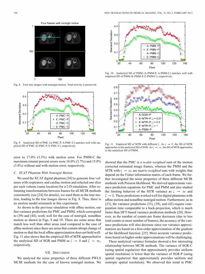
Fig. 8. Four true images with nonrigid motion. Total activity is preserved.

Fig. 9. Analytical SD of PMC (A-PMC-P, A-PMC-C) matches well with em-pirical SD of PMC (E-PMC-P, E-PMC-C), respectively.

error to 17.0% (3.3%) with motion error. For PMM-C themaximum (mean) percent errors were 16.0% (3.7%) and 15.0%(3.8%) without and with motion error, respectively.

C. XCAT Phantom With Nonrigid Motion

We used the XCAT digital phantom [36] to generate four vol-umes with respiratory and cardiac motion and selected one sliceper each volume (same location) for a 2-D simulation. After es-timating transformations between frames for all MCIR methodsconsistently (see [24] for details), we used them as the true mo-tion, leading to the true images shown in Fig. 8. Thus, there isno motion model mismatch in this experiment.As shown in the previous simulation with affine motion, our

fast variance predictions for PMC and PMM, which correspondto (39) and (44), work well for the case of nonrigid, nonaffinemotion as shown in Figs. 9 and 10. There are some areas thatmatch less well than other areas (and compared to the case ofaffinemotion) since there are areas that contain abrupt change ofmotion so that the local affine approximation does not hold well.Fig. 11 also shows that the empirical SD of MTR approached tothe analytical SD of SGR and PMM as and ,respectively.

VII. DISCUSSION

We analyzed the noise properties of three different PWLSMCIR methods for the case of known nonrigid motion. We

Fig. 10. Analytical SD of PMM (A-PMM-P, A-PMM-C) matches well withempirical SD of PMM (E-PMM-P, E-PMM-C), respectively.

Fig. 11. Empirical SD of MTR with different . As , the SD of MTRapproaches to the analytical SD of SGR.As , the SD ofMTR approachesto the analytical SD of PMM.

showed that the PMC is a scalar-weighted sum of the motioncorrected estimated image frames, whereas the PMM and theMTR with are matrix-weighted sum with weights thatdepend on the Fisher information matrix of each frame. We fur-ther investigated the noise properties of three different MCIRmethods with Poisson likelihood. We derived approximate vari-ance prediction equations for PMC and PMM and also studiedthe limiting behavior of the MTR variance as and

. These predictions worked well for digital phantoms withaffine motion and nonaffine nonrigid motion. Furthermore, as in[23], the variance predictions (33), (39), and (42) require com-putation time comparable to a back-projection, which is muchfaster than DFT-based variance prediction methods [20]. How-ever, as the number of counts per frame decreases (due to lesstotal counts or more number of frames), the accuracy of the vari-ance predictions will also decrease since our variance approxi-mations are based on a first-order approximation of the gradientof the likelihood function. [25]. More accurate variance predic-tions based on higher-order approximations will be challenging.These analytical variance formulas showed a few interesting

relationship between MCIR methods. The variance of SGR-C(using spatial regularizer that approximately provides uniformspatial resolution) is lower than the variance of SGR-P (usingspatial regularizer that approximately provides uniform andisotropic spatial resolution). We observed this trend in PMC


and PMM as well. The variance of PMM is less than or com-parable to the variance of PMC and the gap between them willbe larger when the frames have significantly different countsand PMC uses equal scalar weighted sum. When PMC usesproper weights (e.g., normalized scan durations), PMC andPMM empirically had similar variances in our simple phantomsimulation with affine motions. The variance of PMM is alsoless affected by motion than the variance of PMC when the totalactivity preserving condition is used. The variance of MCIRwith frames may not provide times lower variancethan the variance of SGR due to motion. This suggests that onecan choose the reference frame to minimize the variance ofMCIR methods based on this intuition. Lastly, MTR with verylarge usually yields images as good as PMM. However, toolarge can slow convergence of the reconstruction algorithm.When the motion is given, PMM seems to be preferable toPMC and MTR.This paper has focused on the case of known true motion. In

practice motion is never known perfectly and motion errors mayintroduce further bias and/or variability into MCIR results andmotion errors may also degrade the accuracy of noise predic-tions. Our anecdotal results with motion errors in Section VI-Bsuggest that the noise predictions are not highly sensitive tosmall motion errors; in fact the noise predictions seem to be lesssensitive to motion errors than were the regularizer designs forMCIR described in [24]. Methods for reducing motion errorswill of course improve MCIR results, regularizer designs, andnoise prediction accuracy.This analysis can serve as a starting point for understanding

joint estimation of image and motion [12]. Since the Jacobiandeterminant of estimated deformations affects the noise proper-ties, it is important to enforce correct prior knowledge for localvolume changes. Extending this analysis for unknown nonrigidmotion will be interesting future work [40]. Our work has beenfocused on spatial resolution [24] and noise analyses of MCIRmethods; it would also be interesting to extend the work to an-alyze detection performance [41], [42].

APPENDIXPROOF OF THEOREM 1

To prove this theorem, we need to treat the null space ofcarefully. Since the matrix in (18) is symmetric nonneg-ative definite (i.e., positive semidefinite), it has an orthonormaleigen-decomposition of the form

(58)

where the columns of the matrices , are orthonormal and, i.e., is positive definite. The columns of span

the null space of . From the definition of in (16), it isclear that the null space of consists of images that satisfythe following conditions:

...

(59)

for any image . In other words, the matrixhas a null space of dimension . (In contrast, the spatial

regularizer usually has a null space only of dimension 1,which is usually formed of constant images.) We rewrite thesystem of (59) as

(60)

where is defined in (9) and . Evenif we add a periodic condition to (16), then

still has a null space of dimension provided the tran-sitivity property of the motion model holds. Using (60) we canconstruct in (58) as follows:

(61)

where so that is orthonormal. Note that

because and ispositive definite. So, is invertible.Under the usual assumption that and have disjoint null

spaces, one can verify that

(62)

To proceed, we express in (19) as follows:

Thus,

where . By Schur complement [43], we have

(63)

where . Since is positivedefinite, as . Thus, by (62)

(64)

Therefore, as

(65)

REFERENCES[1] G. J. Klein, B. W. Reutter, and R. H. Huesman, “Non-rigid summing

of gated PET via optical flow,” IEEE Trans. Nucl. Sci., vol. 44, no. 4,pp. 1509–1512, Aug. 1997.

[2] M. Dawood, N. Lang, X. Jiang, and K. P. Schafers, “Lung motion cor-rection on respiratory gated 3-D PET/CT images,” IEEE Trans. Med.Imag., vol. 25, no. 4, pp. 476–485, Apr. 2006.

[3] W. Bai and M. Brady, “Regularized B-spline deformable registrationfor respiratory motion correction in PET images,” Phys. Med. Biol.,vol. 54, no. 9, pp. 2719–2736, May 2009.


[4] E. Gravier, Y. Yang, and M. Jin, “Tomographic reconstruction of dy-namic cardiac image sequences,” IEEE Trans. Image Process., vol. 16,no. 4, pp. 932–942, Apr. 2007.

[5] B. A. Mair, D. R. Gilland, and J. Sun, “Estimation of images and non-rigid deformations in gated emission CT,” IEEE Trans. Med. Imag.,vol. 25, no. 9, pp. 1130–44, Sep. 2006.

[6] M. W. Jacobson and J. A. Fessler, “Joint estimation of image and de-formation parameters in motion-corrected PET,” in Proc. IEEE Nucl.Sci. Symp. Med. Im. Conf., 2003, vol. 5, pp. 3290–3294.

[7] F. Qiao, T. Pan, J. W. Clark, and O. R. Mawlawi, “A motion-incorpo-rated reconstruction method for gated PET studies,” Phys. Med. Biol.,vol. 51, no. 15, pp. 3769–3784, Aug. 2006.

[8] T. Li, B. Thorndyke, E. Schreibmann, Y. Yang, and L. Xing, “Model-based image reconstruction for four-dimensional PET,” Med. Phys.,vol. 33, no. 5, pp. 1288–98, May 2006.

[9] K. Taguchi, Z. Sun, W. P. Segars, E. K. Fishman, and B. M. W.Tsui, “Image-domain motion compensated time resolved 4D cardiacCT,” Proc. SPIE 6510, Med. Imag. 2007: Phys. Med. Imag., pp.651016–651016, 2007.

[10] F. Lamare, M. J. L. Carbayo, T. Cresson, G. Kontaxakis, A. Santos,C. C. LeRest, A. J. Reader, and D. Visvikis, “List-mode-based recon-struction for respiratory motion correction in PET using non-rigid bodytransformations,” Phys. Med. Biol., vol. 52, no. 17, p. 5187, Sep. 2007.

[11] F. Odille, N. Cîndea, D. Mandry, C. Pasquier, P.-A. Vuissoz, and J.Felblinger, “Generalized MRI reconstruction including elastic physio-logical motion and coil sensitivity encoding,”Mag. Res. Med., vol. 59,no. 6, pp. 1401–11, Jun. 2008.

[12] S. Y. Chun and J. A. Fessler, “Joint image reconstruction and non-rigid motion estimation with a simple penalty that encourages localinvertibility,” Proc. SPIE 7258, Med. Imag. 2009: Phys. Med. Imag.,pp. 72580U–72580U, 2009.

[13] M. Blume, A. Martinez-Möller, A. Keil, N. Navab, and M. Rafecas,“Joint reconstruction of image and motion in gated positron emissiontomography,” IEEE Trans. Med. Imag., vol. 29, no. 11, pp. 1892–1906,Nov. 2010.

[14] B. Guérin, S. Cho, S. Y. Chun, X. Zhu, N. M. Alpert, G. E. Fakhri,T. Reese, and C. Catana, “Nonrigid PET motion compensation in thelower abdomen using simultaneous tagged-MRI and pet imaging,”Med. Phys., vol. 38, no. 6, pp. 3025–3038, 2011.

[15] C. J. Ritchie, J. Hsieh, M. F. Gard, J. D. Godwin, Y. Kim, and C. R.Crawford, “Predictive respiratory gating: A new method to reduce mo-tion artifacts on CT scans,”Radiology, vol. 190, no. 3, pp. 847–52,Mar.1994.

[16] S. A. Nehmeh, Y. E. Erdi, C. C. Ling, K. E. Rosenzweig, H. Schoder, S.M. Larson, H. A. Macapinlac, O. D. Squire, and J. L. Humm, “Effect ofrespiratory gating on quantifying PET images of lung cancer,” J. Nuc.Med., vol. 43, no. 7, pp. 876–881, Jul. 2002.

[17] R. Manjeshwar, X. Tao, E. Asma, and K. Thielemans, “Motion com-pensated image reconstruction of respiratory gated PET/CT,” in Proc.IEEE Int. Symp. Biomed. Imag., 2006, pp. 674–7.

[18] K. Thielemans, R. Manjeshwar, X. Tao, and E. Asma, “Lesion de-tectability in motion compensated image reconstruction of respiratorygated PET/CT,” in IEEE Nucl. Sci. Symp. Conf. Rec., Nov. 2006, vol.6, pp. 3278–3282.

[19] M. V. W. Zibetti, F. S. V. Bazán, and J. Mayer, “Determining the regu-larization parameters for super-resolution problems,” Signal Process.,vol. 88, no. 12, pp. 2890–2901, 2008.

[20] E. Asma, R. Manjeshwar, and K. Thielemans, “Theoretical compar-ison of motion correction techniques for PET image reconstruction,”in Proc. IEEE Nucl. Sci. Symp. Med. Imag. Conf., 2006, vol. 3, pp.1762–1767.

[21] J. A. Fessler and W. L. Rogers, “Spatial resolution properties of pe-nalized-likelihood image reconstruction methods: Space-invariant to-mographs,” IEEE Trans. Image Process., vol. 5, no. 9, pp. 1346–1358,Sep. 1996.

[22] J. Qi and R. M. Leahy, “Resolution and noise properties of MAP re-construction for fully 3D PET,” IEEE Trans. Med. Imag., vol. 19, no.5, pp. 493–506, May 2000.

[23] Y. Zhang-O’Connor and J. A. Fessler, “Fast predictions of varianceimages for fan-beam transmission tomography with quadratic regular-ization,” IEEE Trans. Med. Imag., vol. 26, no. 3, pp. 335–346, Mar.2007.

[24] S. Y. Chun and J. A. Fessler, “Spatial resolution properties of mo-tion-compensated tomographic image reconstruction methods,” IEEETrans. Med. Imag., vol. 31, no. 7, pp. 1413–1425, Jul. 2012.

[25] J. A. Fessler, “Mean and variance of implicitly defined biased estima-tors (such as penalized maximum likelihood): Applications to tomog-raphy,” IEEE Trans. Imag. Process., vol. 5, no. 3, pp. 493–506, Mar.1996.

[26] M. Elad and A. Feuer, “Restoration of a single superresolution imagefrom several blurred, noisy, and undersampled measured images,”IEEE Trans. Imag. Process., vol. 6, no. 12, pp. 1646–1658, Dec. 1997.

[27] R. Fransens, C. Strecha, and L. Van Gool, “Optical flow based super-resolution: A probabilistic approach,”Comput. Vis. Imag. Understand.,vol. 106, no. 1, pp. 106–115, Apr. 2007.

[28] M. Zibetti and J.Mayer, “A robust and computationally efficient simul-taneous super-resolution scheme for image sequences,” IEEE Trans.Circuits Syst. Video Technol., vol. 17, no. 10, pp. 1288–1300, Oct. 2007.

[29] M. Unser, A. Aldroubi, and M. Eden, “B-spline signal processing: PartI—theory,” IEEE Trans. Signal Process., vol. 41, no. 2, pp. 821–833,Feb. 1993.

[30] P. E. Kinahan, D. W. Townsend, T. Beyer, and D. Sashin, “Attenuationcorrection for a combined 3D PET/CT scannter,” Med. Phys., vol. 25,no. 10, pp. 2046–2053, Oct. 1998.

[31] M. Hofmann, B. Pichler, B. Schlkopf, and T. Beyer, “Towards quan-titative PET/MRI: A review of MR-based attenuation correction tech-niques,” Eur. J. Nucl. Med. Mol. Imag., vol. 36, pp. 93–104, 2009.

[32] H. R. Shi and J. A. Fessler, “Quadratic regularization design for 2-DCT,” IEEE Trans. Med. Imag., vol. 28, no. 5, pp. 645–656, May 2009.

[33] H. H. Barrett and K. J. Myers, Foundations of Image Science. NewYork: Wiley, 2003.

[34] J. W. Stayman and J. A. Fessler, “Compensation for nonuniformresolution using penalized-likelihood reconstruction in space-variantimaging systems,” IEEE Trans. Med. Imag., vol. 23, no. 3, pp.269–284, Mar. 2004.

[35] J. A. Fessler, “Analytical approach to regularization design forisotropic spatial resolution,” in Proc. IEEE Nucl. Sci. Symp. Med.Imag. Conf., 2003, vol. 3, pp. 2022–2026.

[36] W. P. Segars, M. Mahesh, T. J. Beck, E. C. Frey, and B. M. W. Tsui,“Realistic CT simulation using the 4D XCAT phantom,” Med. Phys.,vol. 35, no. 8, pp. 3800–3808, Aug. 2008.

[37] S. Y. Chun and J. A. Fessler, “A simple regularizer for B-spline non-rigid image registration that encourages local invertibility,” IEEE J.Sel. Top. Signal Process., vol. 3, no. 1, pp. 159–169, Feb. 2009.

[38] J. L. Morales and J. Nocedal, “Remark on algorithm 778: L-bfgs-b:Fortran subroutines for large-scale bound constrained optimization,”ACM Trans. Math. Softw., vol. 38, no. 1, pp. 7:1–7:4, Nov. 2011.

[39] S. Becker, L-BFGS-B mex Wrapper Feb. 2012 [Online]. Available:http://www.mathworks.com/matlabcentral/fileexchange/35104

[40] D. Robinson and P. Milanfar, “Statistical performance analysis ofsuper-resolution,” IEEE Trans. Image Process., vol. 15, no. 6, pp.1413–1428, Jun. 2006.

[41] P. Bonetto, J. Qi, and R. M. Leahy, “Covariance approximation for fastand accurate computation of channelized hotelling observer statistics,”IEEE Trans. Nucl. Sci., vol. 47, no. 4, pp. 1567–1572, Aug. 2000.

[42] Y. Xing, I.-T. Hsiao, and G. Gindi, “Rapid calculation of detectabilityin Bayesian single photon emission computed tomography,” Phys.Med. Biol., vol. 48, no. 22, pp. 3755–3774, Nov. 2003.

[43] H. V. Henderson and S. R. Searle, “On deriving the inverse of a sumof matrices,” SIAM Rev., vol. 23, no. 1, pp. 53–60, Jan. 1981.

ieee transactions on medical imaging, vol. 32, no. 2...

Documents