ieee transactions on medical imaging 1 a maximum likelihood

IEEE TRANSACTIONS ON MEDICAL IMAGING 1

A Maximum Likelihood Approach to Parallel

Imaging With Coil Sensitivity Noise

Ashish Raj, Yi Wang and Ramin Zabih

Abstract

Parallel imaging is a powerful technique to speed up Magnetic Resonance (MR) image acquisition via multiple coils.Both the received signal of each coil and its sensitivity map, which describes its spatial response, are needed duringreconstruction. Widely used schemes such as SENSE assume that sensitivity maps of the coils are noiseless while theonly errors are due to a noisy signal. In practice, however sensitivity maps are subject to a wide variety of errors. Atfirst glance, sensitivity noise appears to result in an errors-in-variables problem of the kind that is typically solved usingTotal Least Squares (TLS). However, existing TLS algorithms are inappropriate for the specific type of block structurethat arises in parallel imaging. In this paper we take a maximum likelihood approach to the problem of parallel imagingin the presence of independent Gaussian sensitivity noise. This results in a quasi-quadratic objective function, whichcan be efficiently minimized. Experimental evidence suggests substantial gains over conventional SENSE, especially innon-ideal imaging conditions like low SNR, high g-factors, large acceleration and misaligned sensitivity maps.

Keywords

Parallel imaging, Magnetic Resonance, Maximum Likelihood, SENSE, Total Least Squares.

I. Parallel Imaging and Sensitivity Noise

THE use of multiple coils in MR imaging to substantially reduce scan time (and thus motionartifacts) has become quite popular recently [1]. These paralel imaging techniques are known

as SMASH [2], [3], [4]; SENSE [5], [6], [7] [8]; or GRAPPA [9], [10]. They are closely related to eachother [11], [12]. Mathematically, SENSE is the exact reconstruction method, and will be the focus onthis work. All these schemes use multiple coils to reconstruct the unaliased image from under-sampleddata in Fourier space, also known as k-space. Each coil also has a sensitivity map depicting its spatialresponse over the imaging volume. Aliased data are combined using sensitivity maps to reconstructa full, unaliased image. SENSE is a powerful method to exploit data redundancy from multiple coilsand is rightly considered a major breakthrough in MR imaging. It works superbly in well-behavedsituations with high SNR and low g-factors, but starts to deteriorate under non-ideal conditions. Someof these issues were highlighted in [12].

In this paper we address a major source of errors in SENSE: the situation where it is difficult toobtain artifact-free sensitivity maps. Now sensitivity maps are computed from an MR scan, typicallyof a phantom or after division by a body coil image. As a result, they are subject to similar noiseprocesses that affect the data. In addition, the encoding and decoding sensitivity are not identicalin practical imaging situations involving physiological motion, misalignment of coils between scans,etc. Under modest acceleration, low g-factors and high SNR, these sensitivity effects may not appearto greatly degrade SENSE performance, but our examples suggest that SENSE produces disturbingartifacts when these ideal conditions do not hold. We propose a robust reconstruction which is tolerantto unreliable sensitivity information. This may potentially open up the field of SENSE imaging tosituations where it could not previously be employed. In particulr, preliminary results in section Vindicate strong performance under many challenging conditions like low-SNR sensitivity maps, sensi-tivity misalignment due to coil or physiological movement, high acceleration, and in interior regionswith poor signal penetration and high g-factors.

The authors are with the Radiology Department, Weill Medical College of Cornell University. Ashish Raj is also with Radiology,University of California at San Francisco, and Ramin Zabih is also with the Cornell Computer Science Department. Addresscorrespondence to: Ramin Zabih, 4130 Upson Hall, Cornell University, Ithaca NY 14853, [email protected].


To some extent, the issue of poor SNR was addressed using regularization [13], [14], [15], and theissue of sensitivity noise using a Total Least Squares (TLS) approach [16]. This paper improves,extends and generalizes the TLS work via a Maximum-Likelihood (ML) formulation. We show thatTLS makes assumptions about sensitivity errors which do not occur in general MR imaging practiceexcept under very specific situations. We then obtain new algorithms from basic ML principles whichovercome these problems. The parallel imaging process has a linear form

y = Ex + n, y = Ex + n (1)

The left equation refers to k-space quantities, and the right one image-space. Coil outputs aredenoted by y and y, the desired image by x and x, and imaging noise by n and n. Matrix E containssensitivity and reduced encoding information. 1 A formalization of the imaging process is in section II-A. SENSE reconstruction assumes that n is idependent and identically distributed (i.i.d.) Gaussiannoise. 2 SENSE takes a least squares approach, which is well-known to be the maximum likelihoodestimate under i.i.d. Gaussian assumption[18, Ch. 15]. We will model the imaging process as

y = (E + ∆E)x + n, (2)

where ∆E is the noise in the system matrix that results from errors in the sensitivity maps (i.e., sen-sitivity noise). At first glance, this appears to be an errors-in-variables problem of the kind commonlyaddressed with Total Least Squares (TLS) [19]. Indeed, several authors, such as [16], have suggestedtaking a TLS approach to sensitivity error. However, TLS algorithms assume that ∆E consists ofindependent elements. We will demonstrate in section II-D that this assumption is generally invalid,due to the specific structure of the system matrix E in parallel imaging.

We propose a maximum likelihood (ML) approach to solving Equation (2), which generalizes bothleast squares [18] and total least squares [19]. First we derive the general ML result which is ap-plicable for arbitrary noise models and sampling trajectories, assuming only that there is no cross-coilinterference. Using this as the foundation, we develop practical algorithms for specific situations.

While the general result is valid for any noise model, for practicality we use a natural model wherebysensitivity maps are corrupted by independent (but possibly non-identically distributed) noise. Thismodels many actual imaging situations where sensitivity maps suffer from uncorrelated but spatiallyvarying noise. The resulting algorithm, which we call Maximum Likelihood SENSE or ML-SENSE,gives strong results, even in cases where this noise model is inaccurate. We show examples of spa-tially correlated sensitivity noise which are effectively mitigated by our method. This suggests thatthe independent noise assumption, while not completely adequate, is still much better than the con-ventional assumption of zero sensitivity errors. This is not surprising - for years workers in signalprocessing, radar systems and mobile communications, for examples, have used independent Gaussianmodels to great effect, even in cases where they are demonstrably inaccurate. Note also that SENSEtoo is optimal only for i.i.d. additive Gaussian noise, but has been profitably employed in non-i.i.d.situations.

This paper is organized as follows. The parallel MR acquisition model is detailed in section II forgeneral and special (Cartesian) case, and our sensitivity noise model is introduced. In section III wediscuss related TLS work, and show that they cannot generally handle sensitivity noise. Section IVderives our algorithm using ML principles. For more background and detailed derivations, the readeris referred to [20, Ch. 3]. We show that with Cartesian sampling the general solution reduces to aquasi-quadratic minimization problem directly in image space. We give experimental results on bothsimulated and clinical data in section V.

1We will denote k-space objects by x, and image-space by x.2See [17] for a study of noise in medical imaging.


X Sl yl

.. FTUnder-

Sampling

by R

image-space k-space

X Sl yl

.. FTUnder-

Sampling

by R

image-space k-space

Fig. 1

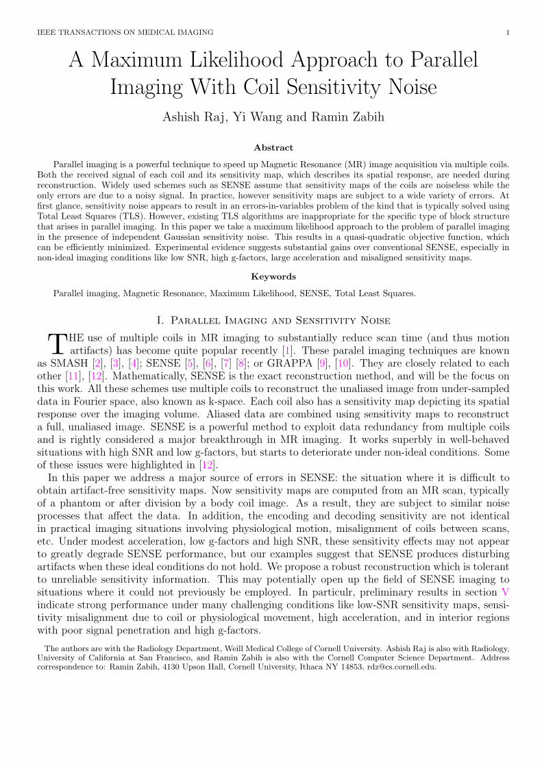
Schematic description of the parallel imaging process for the lth coil. The target image X is

multiplied voxel-by-voxel with the coil sensitivity Sl. After Fourier Transform, the data is in

k-space. Reduced encoding corresponds to undersampling this k-space R times, as shown here for

the Cartesian case.

II. MR acquisition model

In this section we obtain the imaging model summarized in (2). Scalars, vectors and 1D objects aredenoted in lower case; matrices and 2D objects in upper case. Vectors and matrices are in boldface.Unitary or binary scalar operations applied on vectors or matrices are implicitly element-by-elemnt.For instance ‘x · y’ is understood to be element-wise multiply (not the dot product which we denoteby xT y) . The notation diag(x) represents a diagonal matrix whose diagonal elements are given bythose of the enclosed vector x. I is the identity matrix; boldface 1 the vector of ones. Qij denotes the(i, j)-th element of matrix Q; qi the ith element of vector q.

A. System model

The system matrices E and E represent a concatenation over all coils of the discretized encodingoperator which acts on the input image vector x and k-space vector x, respectively. The vector x is adiscrete representation of the desired MR image X(r), where r is the 2-D spatial index. The parallelimaging process for each coil l ∈ 1, . . . , L can be summarized by Figure 1, where Yl is the aliased(folded) image seen by the l-th coil, and Sl is its sensitivity response. Let the 2-D vectors k and rbe points in k-space and image-space respectively. The raw data from individual coils in k-space areYl(k). Then

Yl(k) =

∫

dr e−i2πrkSl(r)X(r). (3)

Following [6] the Fourier Transform above can be replaced by 2D-FT F via Dirac distributionssampled at spatial index ρ:

Yl(k) = F[

∑

ρ

Sl(rρ)X(rρ)δ(r − rρ)

]

(k). (4)

This can be discretized by imposing a Cartesian grid on both r and k. Let vectors x, sl and yl bethe lexicographically stacked versions of the 2-D MR image X, sensitivity responses Sl, and aliasedoutputs Yl respectively, sampled on the regular grid of size N ×M . The 2D-FT now becomes the 2-DDFT and the resampling over k may be accomplished by using a general downsampling operator ink-space. This process is depicted in Figure 1.

The input-output relationship of the l-th coil in Figure 1 is succinctly expressed as a matrix product

yl = Elx = DHN×M⇓RDN×MSl ·X = DH

N×M⇓RDN×Mdiag(sl)x. (5)


The k-space downsampling operator ⇓R resamples k-space according to the specific trajectory usedduring the scan. Here it is basically an indicator function from CN×M to CN×M , with zeros for everyk-space point not sampled by the trajectory. The subscript R denotes the data reduction factor, andsuperscript H the Hermitian operation. The operator DN×M is 2-D DFT over grid (N ×M). Thespecific form of ⇓R will depend on the reduction factor and the sampling method used, but it neednot be explicitly computed. Note that for non-Cartesian trajectories the gridding step must always beunderstood to be implicit in the downsampling operator. For instance, if we denote by G the griddingoperator corresponding to a Kaiser-Bessel kernel, then the modified downsampling operator will begiven by ⇓′

R = ⇓RG. Henceforth we shall assume ⇓R incorporates gridding, if any.

B. System matrix structure under Cartesian k-space sampling

Most MR scans are done on Cartesian grids, considerably simplifying things. The 2-D DFT re-duces to two 1-D DFT’s acting on rows and columns. The general-purpose sampling operator ⇓R inEquation (5) is now redefined as a sub-sampling operator, equivalent to removing rows of k-space.

Writing DN×M = DrowM Dcol

N as the explicit row and column 1-D DFT operations, since ⇓R only actson columns, we have ⇓RDN×M = Drow

M ⇓RDcolN . The output image is now N

R×M , and (5) becomes

yl = (DcolN/R)H⇓RDcol

N diag(sl)x, (6)

This equation can be solved separately for each column. Further, this degenerates into individualL×R aliasing equations, according to Theorem 1.

Theorem 1: Let y(i)l , s

(i)l , x(i) be the i-th column of Yl, Sl, X, and (6) be denoted by yl = Elx

(i).Consider a partitioning of these signals into R aliasing components under Cartesian sampling:

x(i) =

x(i)1

...x(i)

R

, s

(i)l =

s(i)l 1...

s(i)l R

,

whose j-th element is given by x(i)r(j) = x(i)(N

R(r − 1) + j), s

(i)l r(j) = s

(i)l (N

R(r − 1) + j). Then

1.

y(i)l =

R∑

r=1

s(i)l r · x(i)

r.

2. E has a diagonal-block structure containing L×R diagonal blocks:

E = Erl r=1...R

l=1...L

where each sub-block Erl is diagonal, with Er

l = diag(s(i)l,r).

Proof: Proof in Appendix-A.

Theorem 1 is pictorially depicted in Figure 2. To maintain readability, we will henceforth dropcolumn superscript (i). Symbols E, x and y etc. will be used both for arbitrary and Cartesian sampling,their meaning indicated by context. Now each block is diagonal according to Theorem 1, so the


coil 1

coil 2

coil L

R aliases

*

*

*

*

*

**

*

*

*

*

**

*

*

*

*

*

.

.

.

coil 1

coil 2

coil L

(a) (b)

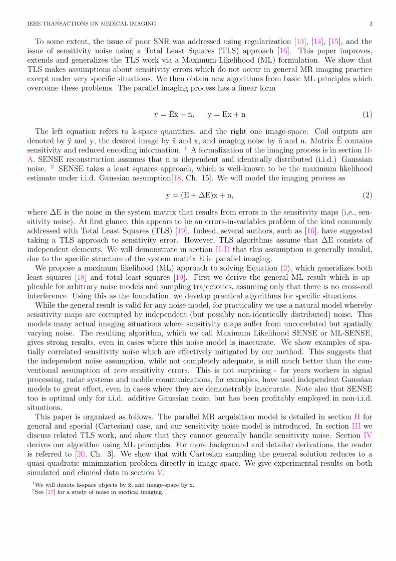
Fig. 2

Structure of system matrix under regular Cartesian sampling. Non-zero elements are indicated

with an asterisk. Part (a) shows E (image space). As a consequence of the partitioning, image

column x(i) separates into R aliasing components. Part (b) shows E, the Fourier dual of E.

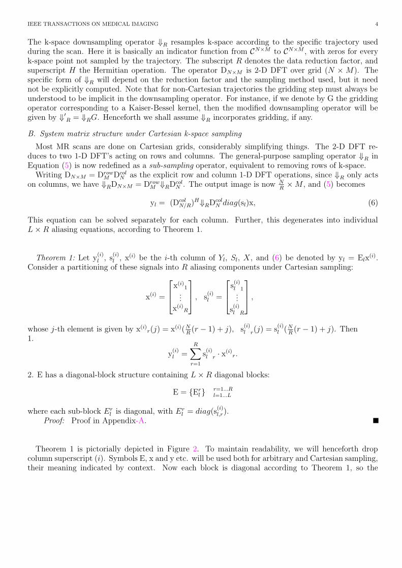
Fig. 3

Converting the full Cartesian problem for each column into a set of independent linear systems

of L observations and R unknowns. Vector µ is L × 1 and η is R × 1; matrix Ψ is L × R. This process is

repeated for every set of R aliasing voxels, and then for each image column.

interactions are restricted to onlyR aliasing voxels at a time. Indeed, define µ ∈ CL, η ∈ CR, Ψ ∈ CL×R.Then for each (j, i)-th voxel in aliased images yl, the SENSE problem becomes:

Given µ(l) = y(i)l (j),

η(r) = x(i)(mod(j, R)),

Ψ(l, r) = s(i)l (mod(j, R)),

Solve µ = Ψη.

This process is pictorially depicted in Figure 3. The process in the figure is repeated for every set ofaliasing voxels, until the entire image is reconstructed.

C. System matrix structure under arbitrary sampling

System matrices E, E have important special forms. Individual blocks E1, . . . ,EL are diagonal, andE1, . . . , EL would have had a Toeplitz structure but for row-decimation due to under-sampling, asshown in Figure 2(b). (Recall that a Toeplitz matrix is a matrix T = Tij such that Tij = tj−i,


which is the (j− i)th element of a row vector t.) The Toeplitz-type structure results from convolutionoperation in k-space. The structure of E for arbitrary sampling can be determined from (5), but isgenerally quite complicated and trajectory-dependent, unlike the simple diagonal Cartesian structure.

D. Our noise model

For practical implementation we will use independent Gaussian noise model for both sensitivity andadditive noise. Note that our reconstruction is complex, hence we do not have to model Rician noisewhich is necessary for magnitude data[17]. The lth coil sensitivity and output noise are modeled as

Snoisyl = Sl +N s

l

Y noisyl = Yl +Nl

where both Nl and N sl are independent Gaussian. Let nl and ns

l be the vectorized representations ofNl and N s

l , with variance given by V ar(nl) = σnωl and V ar(nsl ) = σsλl, where we have introduced

normalized variance vectors ωl and λl. Define for convenience Ωl = diag(ωl), Λl = diag(λl). Then theautocorrelation matrices of output and sensitivity noise are given by

E(nlnlH) = σ2

nΩl2,

E(nsl n

slH) = σ2

sΛl2

Clearly, the structure of 4E must mimic that of E shown in Figure 2(a):

4E = 4Erl r=1...R

l=1...L ,

and the same holds for the k-space versions 4E and E. Again, each sub-block 4Erl is diagonal, with

entries given by the sensitivity map noise terms N sl . Similarly, in k-space the error matrix 4E mimics

the structure of E as shown in Figure 2(b).The assumption of Gaussian noise in spatial sensitivity measurement is quite natural. A popular way

to obtain sensitivity maps is through an initial scan with a uniform phantom. In this case, the effects ofmeasurement noise clearly carry over into sensitivity maps. The effect of this noise can be exacerbatedby further processing, which might introduce its own set of registration and smoothing errors. Anothermethod is to divide the coil outputs by a body coil output [6]. This causes sensitivity errors in regionsof low signal and where the body coil data itself is noisy. The sum-of-squares technique involvesusing densely sampled central k-space to obtain a relative sensitivity map. Both the latter methodsinvolve voxel-wise division, which can be reasonably considered to yield non-identically distributed butstill fairly independent noise. Whenever two separate scans are used for sensitivity and data, certainother small errors such as misregistration due to motion can creep in the sensitivity map estimation.3

All these effects add up, making the independent Gaussian assumption a reasonable one. We willdemonstrate that in the absence of a detailed and exhaustive error model this model suffices.

Our noise model allows for non-identically distributed noise. Noise correlation across coils can beaccomodated by pre-multiplying E with a “whitening” matrix to remove all voxel-wise correlationsamong coils. Pre-whitening for more complicated correlations will generally destroy diagonalization,just as it would in conventional SENSE, leading to greater computational burden. However there isno additional burden in the non-Cartesian case since diagonalization is not available anyway.

III. Related Work

Equation (2) appears to be an errors-in-variables problem of the kind traditionally solved withTLS. Unfortunately TLS makes the unrealistic assumption of independent matrix elemnts. There arevariants of TLS, such as Constrained Total Least Squares, that can handle a broad class of matrixstructure, including the structures that arise in parallel imaging. However, these approaches requirethe use of very general minimization techniques, which are very inefficient.

3This is why we explicitly allow for the noise variance of coil output and coil sensitivity to be different.


A. Total Least Squares

Classical TLS theory [21] applied on (2) attempts to find a solution that minimizes both the additivenoise n as well as the error-in-variables 4E, as follows:

xTLS = arg minx

|| [4E | n] ||F , subject to n + 4Ex = y − Ex (7)

where the indicated norm is Frobenius. This formulation assumes that the elements of 4E are inde-pendent (i.e., that 4E has no structure).

Unfortunately, TLS is ill-equipped to handle the specific system model described in §II. In Cartesiansampling 4E has a diagonal block structure as shown in Figure 2, with off-diagonal elements beingzero. So even if the underlying sensitivity noise process is uncorrelated, the elements of 4E arenever independent (off-digonal entries being identically zero). Thus, the independence assumption ofconventional TLS is generally violated. A similar situation occurs in k-space (1). Matrix 4E has aToeplitz-type structure shown in Figure 2(b). This results in the elements of 4E, being algebraicallyrelated to each other rather than being independent.

The only instance where standard TLS can actually be used in SENSE is for direct unfolding ofaliasing voxels under Cartesian sampling. In this case the problem decouples into independent L×Rsubproblems. This approach was reported in [16]. Unfortunately, there is no k-space equivalent ofthis approach; nor does it extend to non-uniform noise models like those we employ in this paper. Inpractice, it is frequently preferable to reconstruct entire columns or entire image together, for instanceto exploit some a priori knowledge. Non-Cartesian data too must be reconstructed over the entireimage. Direct application of TLS, while conceptually simple, is incompatible with these situations.In contrast, the proposed approach does not have these limitations, and has the added advantage ofstatistical optimality (in ML sense) under a large class of noise models.

B. Constrained Total Least Squares

Several generalizations of TLS, collectively known as Constrained TLS (CTLS), have been proposedto handle matrix structure. 4 CTLS was proposed by [24], whose work handles linearly structured

matrices — those matrices that can be obtained from a linear combinations of a smaller perturbationvector. For a linearly structured matrix E, the CTLS approach works as follows. Define an augmentedmatrix C = [E|y], and a perturbation in C as 4C = [4E|n]. CTLS consists of solving

minv,x

||v||, subject to (C + 4C)

[

x−1

]

= 0 AND 4C = [F1v|F2v| · · · |FN+1v],

where the Fi’s are matrices that generate the elements of ∆C from v. This problem is difficult to solvefor arbitrary E, requiring slow general-purpose constrained minimization techniques.

Matrices described in II turn out to be linearly structured. However, by taking advantage of theparticular structure of the system matrix, we can use much more efficient special-purpose unconstrainedminimization methods. Further details of TLS methods in MR can be found in [20, Ch. 3].

IV. The ML-SENSE Algorithm

We will derive a general sensitivity-error-tolerant reconstruction which maximizes the likelihoodfunction `(x) under arbitrary sampling and general Gaussian noise. Subsequently we obtain a spe-cific efficient algorithm called ML-SENSE, under the independent noise model of section II-D. UnderCartesian sampling this involves minimizing a quasi-quadratic objective function through an efficientnon-linear least squares algorithm.

4An earlier approach, called Structured TLS [22], was shown to be equivalent to CTLS in [23].


A. Deriving the likelihood function `(x)

The likelihood `(x) given the observed data y is defined as Pr(y|x). Let the total noise be g(x) =y−Ex. Under the Gaussian assumption, this is jointly Gaussian with zero mean. As a result we have

`(x) ∝ exp(−1

2(y − Ex)HR−1

g|x(y − Ex)) (8)

where Rg|x = E((g(x))(g(x))H ) is the covariance matrix of the conditional noise g(x)|x.The maximum likelihood estimate, which we will denote x, minimizes − log `(x), and is given by

x = arg minx

(y − Ex)HR−1g|x(y − Ex). (9)

Under our noise model, Rg|x = E(nnH + (4Ex)(4Ex)H), and E(nnH) = σ2nΩ2. We have omitted the

log(det(R−1g|x)) term for tractability, since the log(·) increases slowly compared to the other terms and

is safely neglected. For example, a study of Toeplitz systems in image restoration [25] exhibited littleimprovement after the log term was included, at substantial computational cost. Similar behaviourwas observed during our experimentation. Consequently, we drop this term henceforth.

The data-dependent covariance E((4Ex)(4Ex)H) is an L×L block matrix[

(4Elx)(4El′x)H]

l,l′∈1,...,L

with the (l, l′)-th block given by

(4Elx)(4El′x)H = DHN/R×M⇓RDN×Mdiag(x)E(4sl4sH

l′ )diag(x)DHN×M⇓H

R DN/R×M , (10)

which follows from:

4Elx = DHN/R×M⇓RDN×Mdiag(4sl)x

= DHN/R×M⇓RDN×Mdiag(x)4sl.

Now E(4sl4sHl′ ) = σ2

sδl,l′Λ2l since we assume coils are decoupled, therefore

Rg|x = σ2n

Ω2 + β2

A1(x). . .

AL(x)

, (11)

where Al(x) = DHN/R×M⇓RDN×Mdiag(|Λlx|2)DH

N×M⇓HR DN/R×M , and β = σs/σn.

Finally, we have

R−1g|x =

1

σ2n

B1(x)−1

. . .BL(x)−1

, (12)

Bl(x) = Ω2l + β2DH

N/R×M⇓RDN×Mdiag(|Λlx|2)DHN×M⇓H

R DN/R×M . (13)

Due to the block-diagonality, we can write the maximum likelihood estimate as

x = arg minx

∑

l

(yl − Elx)HBl(x)−1(yl − Elx). (14)

Let us summarize the significance of Equation (14): it provides a general recipe for performingML reconstruction of parallel data under the realistic assumption that noise is present in both coiloutputs as well as sensitivity maps. So far we have not specified any particular model for these noiseprocesses, other than to assume that it is Gaussian and there is no cross-coil interference. In theory,(14) can accomodate any noise model which has an adequate stochastic interpretation in terms ofsecond order statistics captured by Ω and Λ. However, Equation (14) is a non-quadratic minimizationproblem requiring a large number of cost function evaluations over a solution space of extremely largedimensionality. We wish to obtain practical implementations under a more specific and realistic noisemodel discussed in section II-D.


B. Minimization Strategies For General Case

Introducing the independent noise model of section II-D, Ωl and Λl become diagonal, and largesimplifications result. Each function evaluation of (14) for general, arbitrarily sampled data involvesthe inversion of NM ×NM generally non-sparese matrices, making direct inversion prohibitive. How-ever, inversion may be efficiently performed iteratively since the products Bl(x)p and Bl(x)Hp for anarbirary vector p can be computed at O(NM log(N)) cost due to the presence of the Fourier operator.Furthermore, Bl(x) are obviously well-conditioned due to diagonal Ωl and Λl, which means that afast iterative algorithm like Preconditioned CG [21] can perform this inversion in relatively few steps.Since the cost function may be expressed as a data-dependent weighted least squares problem, powerfulnon-linear least squares algorithms can be used to solve the problem efficiently (see [18, Ch. 10]). TheML estimate (14) will not only reduce drastically in complexity.

We do not further specify an implementation for the general case in this paper, focussing insteadon the special but important case of Cartesian sampling to obtain an efficient algorithm.

C. Efficient Algorithm For Cartesian Sampling

Recall that for Cartesian sampling the ML problem can be independently solved for each column (i).Further, we prove in Theorem 2 that both i.i.d. and non-i.i.d. Gaussian cases give diagonal Bl(x

(i)).Hence the ML problem reduces like SENSE (Fig. 3) to NM/R subproblems, each with R variables.

Theorem 2:

For i.i.d. noise: define vectors bl(x(i))

4= 1 + β2

∑Rr=1 |x

(i)r |2, l ∈ 1, . . . , L.

Then the ML estimate (14) of column (i) under Cartesian sampling is given by

x(i) = arg minx

∑

l

‖(y(i)l − s

(i)l,r · x)‖2 / bl(x).

For non-i.i.d. noise with Λ and Ω: The Cartesian ML estimate is given by

x′(i)l

4= λ

(i)l · x(i),

b′l(x

(i))4= ωl

(i)2 + β2

R∑

r=1

|x′l(i)r |2,

x(i) = arg minx

∑

l

‖(y(i)l − s

(i)l,r · x′)‖2 / b′

l(x).

Proof: Note that the division ‘/’ is element-by-element. Proof in Appendix-B.

Now for each aliasing voxel (j, i), define η, µ,Ψ, as before. Then the ML problem reduces to solving

η = arg minη

||F (η)||2, F (η) = q(η)(µ− Ψη), q(η) = 1/√

1 + β2||η||2. (15)

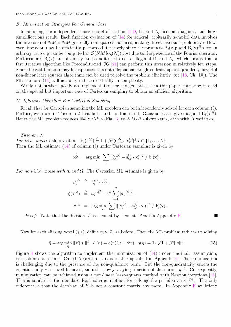
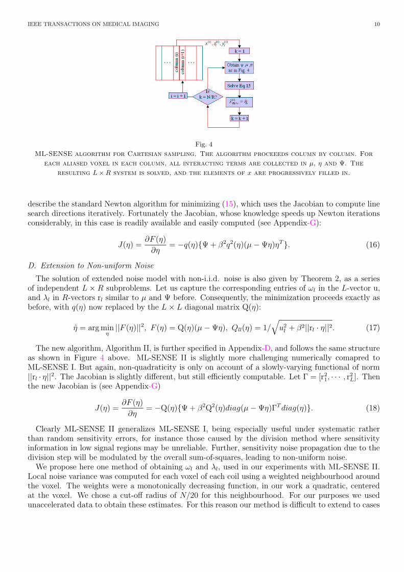
Figure 4 shows the algorithm to implement the minimization of (14) under the i.i.d. assumption,one column at a time. Called Algorithm I, it is further specified in Appendix-C. The minimizationis challenging due to the presence of the non-quadratic term. But the non-quadraticity enters theequation only via a well-behaved, smooth, slowly-varying function of the norm ||η||2. Consequently,minimization can be achieved using a non-linear least-squares method with Newton iterations [18].This is similar to the standard least squares method for solving the pseudoinverse Ψ†. The onlydifference is that the Jacobian of F is not a constant matrix any more. In Appendix-F we briefly


Fig. 4

ML-SENSE algorithm for Cartesian sampling. The algorithm proceeeds column by column. For

each aliased voxel in each column, all interacting terms are collected in µ, η and Ψ. The

resulting L × R system is solved, and the elements of x are progressively filled in.

describe the standard Newton algorithm for minimizing (15), which uses the Jacobian to compute linesearch directions iteratively. Fortunately the Jacobian, whose knowledge speeds up Newton iterationsconsiderably, in this case is readily available and easily computed (see Appendix-G):

J(η) =∂F (η)

∂η= −q(η)Ψ + β2q2(η)(µ− Ψη)ηT. (16)

D. Extension to Non-uniform Noise

The solution of extended noise model with non-i.i.d. noise is also given by Theorem 2, as a seriesof independent L× R subproblems. Let us capture the corresponding entries of ωl in the L-vector u,and λl in R-vectors rl similar to µ and Ψ before. Consequently, the minimization proceeds exactly asbefore, with q(η) now replaced by the L× L diagonal matrix Q(η):

η = arg minη

||F (η)||2, F (η) = Q(η)(µ− Ψη), Qll(η) = 1/√

u2l + β2||rl · η||2. (17)

The new algorithm, Algorithm II, is further specified in Appendix-D, and follows the same structureas shown in Figure 4 above. ML-SENSE II is slightly more challenging numerically comapred toML-SENSE I. But again, non-quadraticity is only on account of a slowly-varying functional of norm||rl · η||2. The Jacobian is slightly different, but still efficiently computable. Let Γ = [r2

1, · · · , r2L]. Then

the new Jacobian is (see Appendix-G)

J(η) =∂F (η)

∂η= −Q(η)Ψ + β2Q2(η)diag(µ− Ψη)ΓTdiag(η). (18)

Clearly ML-SENSE II generalizes ML-SENSE I, being especially useful under systematic ratherthan random sensitivity errors, for instance those caused by the division method where sensitivityinformation in low signal regions may be unreliable. Further, sensitivity noise propagation due to thedivision step will be modulated by the overall sum-of-squares, leading to non-uniform noise.

We propose here one method of obtaining ωl and λl, used in our experiments with ML-SENSE II.Local noise variance was computed for each voxel of each coil using a weighted neighbourhood aroundthe voxel. The weights were a monotonically decreasing function, in our work a quadratic, centeredat the voxel. We chose a cut-off radius of N/20 for this neighbourhood. For our purposes we usedunaccelerated data to obtain these estimates. For this reason our method is difficult to extend to cases


Algorithm SENSE ML-SENSE I ML-SENSE IIflops per iteration O(2MNL) O(3MN(L+ 1)) O(3MN(L+ 2))

avg iterations 10 30 30

TABLE I

Summary of computational burden. The order of flops formulas are theoretical number of

multiplication operations per iteration of the PCG loop. The quoted average number of iterations

are rough estimates obtained empirically from a small number of trials.

where representative unaccelerated scans are not available. More sophisticated methods are currentlybeing investigated; however, we note that in many cases accurate estimates of ωl and λl may notultimately be available. Therefore we describe Algorithms I and II separately – in absence of full noisestatistics, ML-SENSE I is sub-optimal but preferable.

E. Computational Burden

The additional cost of non-quadratic minimization is not significantly higher than standard pseudoin-verse computed through conjugate gradients, due to the easy availability of the Jacobian and its cheapevaluation from (16) and (18). The algorithms were implemented in MATLAB version R13. Typicalexecution times for reconstructions of size 256 × 256 were between three to four times the executiontime in Matlab of standard SENSE. A careful order of flops calculation, contained in Table I, indi-cates a roughly 50% increase in computational burden per iteration. However, ML-SENSE takes moreiterations to converge than SENSE since the former is non-quadratic.

V. Results

Algorithms I and II were not considerably different even under non-i.i.d. noise. ML-SENSE IIseems to perform slightly better when sensitivity errors are spatially varying AND can be properlydetermined; however, it is not possible in many cases to measure this variation accurately. Thereforeboth ML-SENSE I and II are shown in examples below, wherever possible and appropriate. All resultswere compared with conventional SENSE, whose implementation details are supplied in Appendix-E.

A. Simulation results

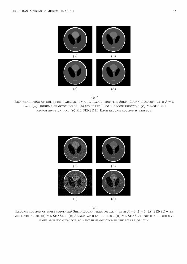
Simulated phased-array data was obtained as follows: Sensitivity of circular coils positioned uni-formly around the FOV were computed from the Biot-Savart Law. Coil data were computed byencoding a fully sampled MR image with coil sensitivities, and down-sampling by R in the PE direc-tion. First reconstruction using SENSE and ML-SENSE is performed on data from a Shepp-Loganhead phantom where both the coil data and simulated sensitivity maps are noiseless. Shown in Figure5, this demonstartes that if there is no sensitivity error, all methods perform perfect reconstruction.

Next we simulation the effect of large Gaussian noise added to data and sensitivity to simulaterandom errors. To keep the comparison uncluttered, equal relative noise was introduced in bothsensitivity and data. The performance of ML-SENSE I with R = 4 and L = 6 can be evaluatedvisually in Figure 6. Since the added noise is uniform, ML-SENSE II results are the same and are notshown here. Reduced phase encoding was along the vertical direction. The standard SENSE result isalmost useless in this case. The encoding matrix is badly conditioned due to large acceleration factor,causing severe noise amplification. In contrast our ML-SENSE algorithm is able to salvage more usefuldata.

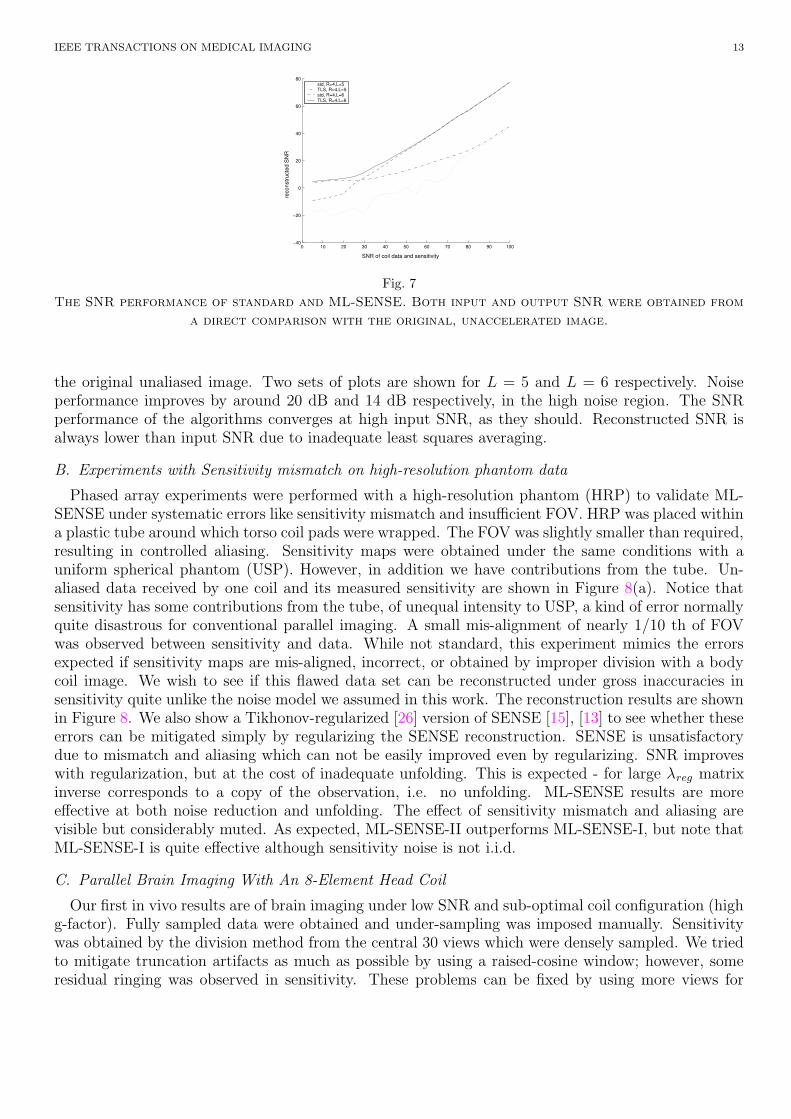
A quantitative comparison is now performed for R = 4. For a given SNR (labeled “input SNR”in Figure 7) of sensitivity and data, we determine the SNR of reconstructions using standard andML-SENSE (labeled “reconstructed SNR”). Reconstructed SNR is available from the difference from


(a) (b)

(c) (d)

Fig. 5

Reconstruction of noise-free parallel data simulated from the Shepp-Logan phantom, with R = 4,

L = 6. (a) Original phantom image, (b) Standard SENSE reconstruction, (c) ML-SENSE I

reconstruction, and (d) ML-SENSE II. Each reconstruction is perfect.

(a) (b)

(c) (d)

Fig. 6

Reconstruction of noisy simulated Shepp-Logan phantom data, with R = 4, L = 6. (a) SENSE with

mid-level noise, (b) ML-SENSE I, (c) SENSE with large noise, (d) ML-SENSE I. Note the excessive

noise amplification due to very high g-factor in the middle of FOV.


0 10 20 30 40 50 60 70 80 90 100−40

−20

0

20

40

60

80

SNR of coil data and sensitivity

reco

nstru

cted

SN

R

std, R=4,L=5TLS, R=4,L=5std, R=4,L=6TLS, R=4,L=6

Fig. 7

The SNR performance of standard and ML-SENSE. Both input and output SNR were obtained from

a direct comparison with the original, unaccelerated image.

the original unaliased image. Two sets of plots are shown for L = 5 and L = 6 respectively. Noiseperformance improves by around 20 dB and 14 dB respectively, in the high noise region. The SNRperformance of the algorithms converges at high input SNR, as they should. Reconstructed SNR isalways lower than input SNR due to inadequate least squares averaging.

B. Experiments with Sensitivity mismatch on high-resolution phantom data

Phased array experiments were performed with a high-resolution phantom (HRP) to validate ML-SENSE under systematic errors like sensitivity mismatch and insufficient FOV. HRP was placed withina plastic tube around which torso coil pads were wrapped. The FOV was slightly smaller than required,resulting in controlled aliasing. Sensitivity maps were obtained under the same conditions with auniform spherical phantom (USP). However, in addition we have contributions from the tube. Un-aliased data received by one coil and its measured sensitivity are shown in Figure 8(a). Notice thatsensitivity has some contributions from the tube, of unequal intensity to USP, a kind of error normallyquite disastrous for conventional parallel imaging. A small mis-alignment of nearly 1/10 th of FOVwas observed between sensitivity and data. While not standard, this experiment mimics the errorsexpected if sensitivity maps are mis-aligned, incorrect, or obtained by improper division with a bodycoil image. We wish to see if this flawed data set can be reconstructed under gross inaccuracies insensitivity quite unlike the noise model we assumed in this work. The reconstruction results are shownin Figure 8. We also show a Tikhonov-regularized [26] version of SENSE [15], [13] to see whether theseerrors can be mitigated simply by regularizing the SENSE reconstruction. SENSE is unsatisfactorydue to mismatch and aliasing which can not be easily improved even by regularizing. SNR improveswith regularization, but at the cost of inadequate unfolding. This is expected - for large λreg matrixinverse corresponds to a copy of the observation, i.e. no unfolding. ML-SENSE results are moreeffective at both noise reduction and unfolding. The effect of sensitivity mismatch and aliasing arevisible but considerably muted. As expected, ML-SENSE-II outperforms ML-SENSE-I, but note thatML-SENSE-I is quite effective although sensitivity noise is not i.i.d.

C. Parallel Brain Imaging With An 8-Element Head Coil

Our first in vivo results are of brain imaging under low SNR and sub-optimal coil configuration (highg-factor). Fully sampled data were obtained and under-sampling was imposed manually. Sensitivitywas obtained by the division method from the central 30 views which were densely sampled. We triedto mitigate truncation artifacts as much as possible by using a raised-cosine window; however, someresidual ringing was observed in sensitivity. These problems can be fixed by using more views for


sensitivity estimation; however, doing so will reduce the effective acceleration and negate the purposeof doing parallel imaging. Further degradation of sensitivity resulted from noise amplification duringthe division step in regions with low signal. This example is a faithful reproduction of typical imagingerrors under challenging imaging conditions. We first show the case of R = 2 times accelaration inFigure 9. Although data and sensitivity maps are error-prone, the results from both SENSE andML-SENSE look acceptable due to low g-factor, with ML-SENSE (c-d) showing a small improvementover both SENSE (a) and its regularized version (b). Now consider the same data, but with R = 4,shown in Figure 10. SENSE reconstruction in (a) now exhibits excessive noise amplification due toa combination of high R and erroneous sensitivity maps. In order to demonstrate that this problemcannot really be addressed by regularized SENSE, (b) shows the output of a Tikhonov-regularizedSENSE algorithm, with λreg = 0.1, chosen after an exhaustive L-curve analysis [13] by varying λreg inincrements given by a geometric progression from 0 to 1. At each increment a data and a prior costwere computed:

Edata = ||y − Ex||2, Eprior = ||x||2.Figure 11 plots these values and is called the L-curve. This is zero-th order regularization since

it does not use a prior mean image [14]. In most interesting situations a prior mean image is notavailable. In our experience means computed from central k-space data produced severe boundaryartifacts. Even in dynamic imaging, mean priors are useful only if the variance from mean is small.

While regularized SENSE, which was previously proposed for parallel imaging by several authors[13], [15], [16] is less noisy, it has in fact failed to resolve the aliasing components properly. A smallerλreg, say 0.05, would have resolved the ghosting better, but with more noise amplification, as impliedby the L-curve. Figure 10(c)&(d) show the ML-SENSE reconstructions, which seem to suffer neitherfrom excessive noise amplification nor ghosting. ML-SENSE II is slightly better than ML-SENSE I asexpected. Comparing Figures 9 and 10, we conclude that while under benign imaging conditions (lowR, small g-factors) sensitivity errors may not impact quality, at higher accelerations and poorer matrixconditioning properties they can seriously degrade conventional performance. In these situations, theML-SENSE approach appears to perform better.

D. Imaging Experiments Under Non-Uniform Sensitivity Noise

Now we investigate the comparative performance of Algorithms I and II for the Shepp-Logan dataset. Sensitivity was obtained from central k-space, and additional perturbations were introduced viashifts in orientation and positioning between the encoding and decoding sensitivities. The resultingsensitivity noise is mostly negligible except within the bright outer ring of the phantom. ML-SENSEI is not likely to produce significant improvement due to the nature of sensitivity errors in this case.However, modeling this as spatially varying noise, reliable estimates of Ω and Λ are available from thesimulation, and we expect ML-SENSE II to provide a better reconstruction. This was found to be thecase, as shown in Figure 12.

Next we investigate the non-uniform sensitivity noise resulting from mis-registration due to breath-ing, a constant problem in torso scanning. An axial torso slice with 3x speed-up was scanned usingthe 8-channel head coil described earlier. The central 30 k-space views were scanned densely, allowingus to obtain unaliased low-frequency sensitivity maps by the division method. In addition to mis-registration, spatially variable sensitivity error was observed due to division in areas of weak signal.ML-SENSE- II is the appropriate method in this case. We obtained Λ and Ω by the local windowvariance estimation described earlier. Results are shown in Figure 13(a) and (b), along with zoomed inregion containing the stomach-heart interface in (c) and (d). Several artifacts contaminate the SENSEoutput, including loss of heart-stomach boundary definition, hyperintensity in heart reion, and stripeartifact across the liver. These artifacts are largely absent in the reconstruction using ML-SENSE II.


VI. Conclusions

We addressed the problem of obtaining an optimal solution to the parallel imaging reconstructionproblem in the presence of both measurement and sensitivity noise. We showed that for independentGaussian noise the optimal solution is the minimizer of a weakly non-quadratic objective functionwhich may be solved efficiently via a non-linear least squares iterative technique with modest additionalcomplexity compared to standard SENSE algorithms. We have also derived simplified expressions forthe cost function as well as the Jacobian of the associated least squares problem in the case of Cartesiank-space sampling. A fast Newton algorithm with explicit Jacobian information was developed to solvethe problem. Results for Cartesian k-space sampling indicate impressive improvement in performancecompared to standard SENSE, amounting to almost 20 dB SNR gain in several high-noise cases. Thealgorithm yields substantial improvement even in cases where the sensitivity noise is not independent.These preliminary results are promising, especially for abdominal imaging where large motion-inducedsensitivity artifacts are present. But the algorithm need to be further evaluated under various clinicalsettings to assess its true clinical significance.

A natural extension to our work would be to handle non-Cartesian sampling schemes. The basicsolution for the ML estimate remains the same, but the non-Cartesian problem can not benefit fromdiagonalization. Efficient implementations for arbitrary sampling as well as for more general noisemodels was briefly described in this paper, but detailed implementation is currently being investigated.

Appendices

A. Proof of Theorem 1

Consider the 1D DFT matrix DcolN = e i2π

N(kn), k = 0 . . . N − 1, n = 0, . . . N − 1. Now the row-

decimated matrix obtained by retaining every Rth row in DcolN can be written as e i2π

N(Rk′n), k′ =

0 . . . N/R − 1, n = 0, . . . N − 1. Expanding this in terms of (N/R × N/R)-blocks, we get, for k ′ =0 . . . N/R− 1, n′ = 0 . . . N/R− 1

⇓RDcolN = e i2π

N(Rk′n′), e

i2π

N(Rk′(n′+N

R)), . . . , e

i2π

N(Rk′(n′+(R−1) N

R)).

Each of these terms evaluates to exp(i 2πN/R

k′n′), giving us

⇓RDcolN = Dcol

N/R[IN/R · · · IN/R], (19)

Therefore y(i)l = Elx

(i) = [IN/R · · · IN/R] diag(s(i)l )x(i) = [diag(s

(i)1 ), · · · , diag(s(i)

R )] x(i).This proves part (1) and leads immediately to the partitioning El = [E1

l , . . . ,ERl ], with Er

l =

diag(s(i)l,r). Assembling the full matrix E for all coils we get the result in part (2).

B. Proof of Theorem 2

Proof: For i.i.d. case, Λ = I, Ω = I. Recall that ⇓RDN×M = DrowM ⇓RDcol

N and DcolN/R

H⇓RDcolN =

[IN/R · · · IN/R] from Theorem 1. Then we have for the column-wise matrix Bl(x(i)) (see Eqn. (13)):

Bl(x(i)) = I + β2 Dcol

N/R

H⇓RDcolN/R diag(|x(i)|2) Dcol

N/R

H⇓HR Dcol

N/R

= I + β2 [IN/R · · · IN/R] diag(|x(i)|2) [IN/R · · · IN/R]T

= diag(1 + β2

R∑

r=1

|x(i)r |2) 4

=[

diag(bl(x(i)))

]−1

Then the ML problem (14) for a single column becomes

x(i) = arg minx

∑

l

(y(i)l − Elx)H [diag(bl(x))]−1 (y

(i)l − Elx)


which immediately proves part (1) of the theorem. Part (2) for non-i.i.d. case follows analogously, thistime accounting for the diagonal matrices Λ and Ω.

C. ML-SENSE Algorithm For Cartesian Sampling: ML-SENSE I

• Yl = coil output of lth coil, in spatial domain• Sl = sensitivity map of lth coil• X = desired MR image of size (N ×M)• L = number of coils• R = downsampling factor.• for i = 1 . . .M1. Define x,yl,sl as the ith column of X,Yl,Sl, respectively.2. for k = 1 . . . N/R(a) Define a L×R matrix Ψ, with Ψl,r = sl,(r−1)N/R+k. Let µ = [y1,k, . . . yL,k]

T .(b) Solve η = arg minη(

11+β2||η||2

)||µ− Ψη||2(c) x(r−1)N/R+k = ηr

3. ith column of X = x.

D. ML-SENSE Under Non-Uniform Sensitivity And Output Noise: ML-SENSE II

• for i = 1 . . .M1. Define x,yl,sl as the ith column of X,Yl,Sl, respectively.2. for k = 1 . . . N/R(a) Define L×R matrix Ψ, with Ψl,r = sl,(r−1)N/R+k.

(b) For each l = 1, . . . , L, define R-vectors rl = λ(r−1)N/R+k,il and ul = ωk,i

l .(c) Define L×R matrix Γ, with Γ = [r2

1, · · · , r2L].

(d) Define µ = [y1,k, . . . yL,k]T .

(e) Solve η = arg minη||Q(η)(µ− Ψη)||2, with Qll = 1√u2

l+β2||rl·η||2

(f) x(r−1)N/R+k = ηr

3. ith column of X = x.

E. SENSE and Regularized SENSE Implementation

Each L×R sub-system µ = Ψη is solved separately in SENSE, then the elements of the full image Xare filled in from the estimates of η. Matrix Ψ is inverted through the pseudo-inverse via the popularConjugate Gradients algorithm described previously by many authors, e.g. [5] and [6]. Thus

η = Ψ†µ.

Regularization: Tikhonov-regularized SENSE was implemented by solving the augmented system

η = Ψ′†µ′ , where

µ′ =[

µT , 0T]T

Ψ′ =[

ΨT , λreg IT]T


F. ML-SENSE Cost Minimization Routine

The minimization of Eqs. (15) and (17) proceeeds via the well-established Gauss-Newton method[27]. In the approximate vicinity of the true solution, the Hessian is given by

H(η) ≈ J(η)TJ(η).

The Gauss-Newton method computes, at each iteration k, a line search direction dk starting fromteh current solution ηk which is the minimizer of the following least squares problem:

mindk

||J(ηk)dk − F (ηk)||2.

Since the Jacobian and function evaluations are explicitly available and cheaply computable viaEqs. (15) – (18), the above is a simple least squares problem which was solved by conventional CGalgorithm. Finally, a one-dimensional line search is performed for each direction dk using the standardmethod described in Section 2-6 of [27].

G. Jacobian Of F (η)

Let ri, Γ be as defined in § IV-D, let the ith element of F (η) be Fi(η), and ith row of Ψ be ψTi . Then

∂Fi(η)

∂η= −Qii(η)ψi +

∂Qii(η)

∂η(µi + ψT

i η)

Now ∂Qii(η)∂η

= −β2Q3ii(η)(r

2i · η). Then

Ji(η) =

(

∂Fi(η)

∂η

)T

= −Qii(η)ψTi + β2Q2

ii(η)(µi + ψTi η)η

Tdiag(r2i )

For algorithm I, r2i = 1, Qii(η) = q(η), and we get

J(η) =

J1(η)...

JL(η)

= −q(η)Ψ + β2q2(η)(µ+ Ψη)ηT.

For algorithm II we need to stack rows Ji(η) more carefully. It is easily verified that

J(η) = −Q(η)Ψ + β2Q2(η)diag(µ− Ψη)ΓTdiag(η).

References

[1] Florian Wiesinger, Peter Boesiger, and Klaas Pruessmann, “Electrodynamics and ultimate SNR in parallel MR imaging,”Magnetic Resonance in Medicine, vol. 52, no. 2, pp. 376–390, August 2004.

[2] D. K. Sodickson and W. J. Manning, “Simultaneous acquisition of spatial harmonics (smash): fast imaging with radiofre-quency coil arrays,” Magnetic Resonance in Medicine, vol. 38, no. 4, pp. 591–603, 1997.

[3] C. A. McKenzie, M. A. Ohliger, E. N. Yeh, M. D. Price, and D. K. Sodickson, “Coil-by-coil image reconstruction withSMASH,” Magnetic Resonance in Medicine, vol. 46, pp. 619–623, 2001.

[4] D. K. Sodickson, C. A. McKenzie, M. A. Ohliger, E. N. Yeh, and M. D. Price, “Recent advances in image reconstruction,coil sensitivity calibration, and coil array design for smash and generalized parallel mri,” Magnetic Resonance Materials inBiology, Physics and Medicine, vol. 13, no. 3, pp. 158–63, 2002.

[5] K. P. Pruessmann, M. Weiger, M. B. Scheidegger, and Peter Boesiger, “SENSE: sensitivity encoding for fast MRI,” MagneticResonance in Medicine, vol. 42, no. 5, pp. 952–962, 2001.

[6] K. P. Pruessmann, M. Weiger, Peter Boernert, and Peter Boesiger, “Advances in sensitivity encoding with arbitrary k-spacetrajectories,” Magnetic Resonance in Medicine, vol. 46, pp. 638–651, 2001.

[7] M. Weiger, K. P. Pruessmann, and P. Boesiger, “2d sense for faster 3d mri,” Magnetic Resonance Materials in Biology,Physics and Medicine, vol. 14, no. 1, pp. 10–19, 2002.

[8] Johan S. van den Brink, Yuji Watanabe, Christian K. Kuhl, Taylor Chung, Raja Muthupillai, Marc Van Cauteren, KeiYamada, Steven Dymarkowski, Jan Bogaert, Jeff H. Maki, Celso Matos, Jan W. Casselman, and Romhild M. Hoogeveen,“Implications of SENSE MR in routine clinical practice,” European Journal of Radiology, vol. 46, no. 1, pp. 3–27, April 2003.


[9] M. A. Griswold, P. M. Jakob, R. M. Heidemann, M. Nittka, V. Jellus, J. Wang, B. Kiefer, and A. Haase, “Generalizedautocalibrating partially parallel acquisitions (grappa),” Magnetic Resonance in Medicine, vol. 47, no. 6, pp. 1202–10, 2002.

[10] B. J. Wintersperger, K. Nikolaou, O. Dietrich, J. Rieber, M. Nittka, M. F. Reiser, and S. O. Schoenberg, “Single breath-holdreal-time cine MR imaging: improved temporal resolution using generalized autocalibrating partially parallel acquisition(GRAPPA) algorithm,” European Journal of Radiology, vol. 13, no. 8, pp. 1931–1936, May 2003.

[11] Yi Wang, “Description of parallel imaging in mri using multiple coils,” Magnetic Resonance in Medicine, vol. 44, pp. 495499,2000.

[12] M. Blaimer, F. Breuer, M. Mueller, R. M. Heidemann, M. A. Griswold, and P. M. Jakob, “Smash, sense, pils, grappa: howto choose the optimal method,” Top. Magnetic Resonance Imaging, vol. 15, no. 4, pp. 223–36, 2004.

[13] F. Lin, K. Kwang, J. Belliveau, and L. Wald, “Parallel imaging reconstruction using automatic regularization,” MagneticResonance in Medicine, vol. 51, no. 3, pp. 559–567, 2004.

[14] K. King and L. Angelos, “Sense image quality improvement using matrix regularization,” in Proc. ISMRM, 2001, p. 1771.[15] R. Bammer, M. Auer, S. L. Keeling, M. Augustin, L. A. Stables, R. W. Prokesch, R. Stollberger, M. E. Moseley, and

F. Fazekas, “Diffusion tensor imaging using single-shot sense-epi,” Magnetic Resonance in Medicine, vol. 48, pp. 128–136,2002.

[16] Z. P. Liang, R. Bammer, J. Ji, N. Pelc, and G. Glover, “Making better sense: Wavelet denoising, Tikhonov regularization,and total least squares,” in Proc. ISMRM, 2002, p. 2388.

[17] P. Gravel, G. Beaudoin, and J. A. DeGuise, “A method for modeling noise in medical images,” IEEE Transactions onMedical Imaging, vol. 23, no. 10, pp. 1221–1232, October 2004.

[18] William Press, Saul Teukolsky, William Vetterling, and Brian Flannery, Numerical Recipes in C, Cambridge, 2nd edition,1992.

[19] Sabine Van Huffel and Philippe Lemmerling, Total Least Squares and Errors-in-Variables Modeling: Analysis, Algorithmsand Applications, Kluwer, 2002.

[20] Ashish Raj, A Signal Processing And Machine Vision Approach to Problems in Magnetic Resonance Imaging, Ph.D. thesis,Cornell University, January 2005.

[21] G. Golub and C. Van Loan, Matrix Computations, Johns Hopkins University Press, 1996.[22] Vladimir Z. Mesarovic, Nikolas P. Galatsanos, and Aggelos K. Katsaggelos, “Regularized Constrained Total Least Squares

image restoration,” IEEE Transactions on Image Processing, vol. 4, no. 8, pp. 1096–1108, August 1995.[23] Philippe Lemmerling, Bart de Moor, and Sabine Van Huffel, “On the equivalence of Constrained Total Least Squares and

Structured Total Least Squares,” IEEE Transactions on Signal Processing, vol. 44, pp. 2908–2911, November 1996.[24] Theagenis J. Abatzoglou, Jerry M. Mendel, and Gail A. Harada, “The Constrained Total Least Squares technique and its

applications to harmonic superresolution,” IEEE Transactions on Signal Processing, vol. 39, no. 5, pp. 1070–1087, May 1991.[25] Vladimir Z. Mesarovic, Nikolas P. Galatsanos, and M. N. Wernick, “Iterative maximum a posteriori (map) restoration from

partially-known blur for tomographic reconstruction,” in ICIP, 1995, pp. 512–515.[26] D. Terzolpoulos, “Regularization of inverse visual problems involving discontinuities,” IEEE Transactions in Pattern Analysis

and Machine Intelligence, vol. PAMI-8, pp. 413–424, July 1986.[27] R. Fletcher, Practical Methods of Optimization, John Wiley and Sons, 1987.


50 100 150 200 250

50

100

150

200

250

50 100 150 200 250

50

100

150

200

250

(a) (b)

(c) (d)

(e) (f)

Fig. 8

Reconstruction results of HiRes data, with R = 3, L = 4: (a) shows (unaliased) output of the HiRes

phantom within the plastic tube, as seen by one of the coils, and (b) shows the corresponding coil

sensitivity map obtained from a uniform phantom using identical geometrical setups for both the

SENSE and the calibration scan. (c) Standard SENSE, (d) Standard SENSE with regularization

factor of 0.05, (e) ML-SENSE-I, and (f) ML-SENSE-II. Both ML-SENSE algorithms exhibit superior

performance compared to conventional methods.


(a) (b)

(c) (d)

Fig. 9

Brain reconstruction results with R = 2, L = 8: (a) SENSE, (b) SENSE regularized with best

parameter from Fig. 11. (c) ML-SENSE-I, and (d) ML-SENSE-II. All algorithms appear similar.

(a) (b)

(c) (d)

Fig. 10

Brain reconstruction with R = 4, L = 8: (a) SENSE, (b) regularized SESNE, (c) ML-SENSE-I, and (d)

ML-SENSE-II. Higher acceleration has caused serious artifacts in conventional methods.

ML-SENSE II seems to better suppress residual aliasing arising from the hyper-intense fat signal.


0 4000 80001000

1200

1400

1600

Edata

Epr

ior

λ = 0.1

λ << 0.1

λ >> 0.1

Fig. 11

L-curve for brain data obtained by varying λreg in increments of a geometric progression from 0 to

1. This is a plot of the prior cost versus data cost. The best value, given by the L-curve elbow,

was around λreg = 0.1. This was used to regularize SENSE in Figure 10.

(a) (b) (c)

Fig. 12

Reconstruction of Shepp-Logan phantom, with R = 2, L = 4 using sensitivity maps obtained from

central (15 × 15) region of k-space and division by sum of squares. Sensitivity was perturbed by

small shifts in orientation and positioning. (a), (b), (c) are SENSE, ML-SENSE I and ML-SENSE II

respectively. Note the absence of the aliasing ring, pointed out by the arrows, in (c).


(a) (b)

(c) (d)

Fig. 13

Reconstruction results of torso scan, R = 3, L = 8 : (a) Standard SENSE with regularization, (b)

ML-SENSE II, (c) Zooming into (a), and (d) Zooming into (b). Note the distortions at the

heart-stomach boundary and strip artifact across the liver in SENSE output.

ieee transactions on medical imaging 1 a maximum likelihood

Documents