ieee transactions on image processing, vol. 24, no. 11 ...jsyuan/papers/2015... · matrices, visual...

IEEE TRANSACTIONS ON IMAGE PROCESSING, VOL. 24, NO. 11, NOVEMBER 2015 3729

Manifold Kernel Sparse Representation ofSymmetric Positive-Definite Matrices

and Its ApplicationsYuwei Wu, Yunde Jia, Member, IEEE, Peihua Li, Jian Zhang, Senior Member, IEEE,

and Junsong Yuan, Senior Member, IEEE

Abstract— The symmetric positive-definite (SPD) matrix, asa connected Riemannian manifold, has become increasinglypopular for encoding image information. Most existing sparsemodels are still primarily developed in the Euclidean space. Theydo not consider the non-linear geometrical structure of the dataspace, and thus are not directly applicable to the Riemannianmanifold. In this paper, we propose a novel sparse representationmethod of SPD matrices in the data-dependent manifold kernelspace. The graph Laplacian is incorporated into the kernel spaceto better reflect the underlying geometry of SPD matrices. Underthe proposed framework, we design two different positive definitekernel functions that can be readily transformed to thecorresponding manifold kernels. The sparse representationobtained has more discriminating power. Extensive experimentalresults demonstrate good performance of manifold kernel sparsecodes in image classification, face recognition, and visualtracking.

Index Terms— Kernel sparse coding, Riemannian manifold,region covariance descriptor, symmetric positive definitematrices, visual tracking, image classification, face recognition.

I. INTRODUCTION

SPARSE representation (SR) has been an important subjectin signal processing and computer vision communities

with a wide range of applications including visualtracking [1]–[3], face recognition [4], [5], and image classifica-tion [6], [7]. Given a set of data points X = {x1, x2, · · · , xn},the sparse model attempts to find a dictionary D ={d1, d2, · · · , dN }, where di is the so-called base or atom,

Manuscript received September 2, 2014; revised February 12, 2015 andMay 9, 2015; accepted June 22, 2015. Date of publication July 1, 2015; date ofcurrent version July 23, 2015. This work was supported in part by the NationalNatural Science Foundation of China under Grant 61375044, in part by theSpecialized Research Fund for the Doctoral Program of Higher Educationof China under Grant 20121101110035, and in part by the Ministry ofEducation Tier-1, Singapore, under Grant M4011272.040. The associate editorcoordinating the review of this manuscript and approving it for publicationwas Prof. Rebecca Willett. (Corresponding author: Yunde Jia.)

Y. Wu and Y. Jia are with the Beijing Laboratory of Intelligent InformationTechnology, School of Computer Science, Beijing Institute of Technology,Beijing 100081, China (e-mail: [email protected]; [email protected]).

P. Li is with the School of Information and CommunicationEngineering, Dalian University of Technology, Dalian 116023, China(e-mail: [email protected]).

J. Zhang is with the Faculty of Engineering and Information Technology,Advanced Analytics Institute, University of Technology at Sydney, Sydney,NSW 2007, Australia (e-mail: [email protected]).

J. Yuan is with the School of Electrical and Electronics Engineering,Nanyang Technological University, Singapore (e-mail: [email protected]).

Color versions of one or more of the figures in this paper are availableonline at http://ieeexplore.ieee.org.

Digital Object Identifier 10.1109/TIP.2015.2451953

such that each xi can be linearly reconstructed by arelatively small subset of atoms from D, meanwhile keepingthe reconstruction error as small as possible. The underlyinglinear process significantly depends on the assumption thatthe data points and the atoms lie on a vector space R

d .In many applications, however, data points actually belong toknown Riemannian manifolds such as the space of symmetricpositive-definite (SPD) matrices [8], [9], Stiefel and Grass-mann manifolds [10], [11]. Most existing sparse models inR

d fail to consider the non-linear geometrical structure of themanifold space M, and hence are not directly applicable tothe Riemannian manifold. In this paper, we tackle the problemof the SR in the space of d × d SPD matrices, denotedby Sym+

d . Unlike the Euclidean space, the space of Sym+d

lacks a global linear structure. To formulate the sparse repre-sentation on Sym+

d , one natural and crucial question arises:how to allow the SPD matrix to be reconstructed linearly bythe atoms on Sym+

d using an appropriate metric which canmeasure the intrinsic distance between two SPD matrices?

Intuitively, a direct approach is to approximate a SPD matrixby the linear combination of other SPD matrices. In general,employing the linear combination of atomic matrices to rep-resent a SPD matrix largely depends on an appropriate metricto measure the reconstruction error, e.g., Logdet divergenceand Frobenius norm. Sivalingam et al. [12] proposed a tensorsparse coding method, in which the Logdet divergence is usedto measure the reconstruction error. The sparse decomposi-tion of a SPD matrix is then formulated as a MAXDEToptimization problem that can be solved by the interior-point (IP) algorithm. Sivalingam et al. [13] further introduceda dictionary learning method using the Logdet divergence.However, the solutions of the above two approaches arecomputationally expensive. Sra and Cherian [14] adopted theFrobenius norm as an error metric to learn a generalizeddictionary of rank-1 atoms to sparsely represent a SPD matrix.However, several studies [15], [16] show that the Frobeniusnorm, which basically vectorizes SPD matrices and measuresthe norm between two matrices, is not a good metric, since itdiscards the manifold geometry.

In order to apply existing vector-based sparsity modelingapproaches, an alternative scheme is to embed manifold datapoints into a vector space R

d . One commonly used vectorspace is the tangent space at the mean of the data pointsin M. The logarithmic and exponential maps are iteratively

1057-7149 © 2015 IEEE. Personal use is permitted, but republication/redistribution requires IEEE permission.See http://www.ieee.org/publications_standards/publications/rights/index.html for more information.

3730 IEEE TRANSACTIONS ON IMAGE PROCESSING, VOL. 24, NO. 11, NOVEMBER 2015

used to map the manifold data points to the tangent space,and vice-versa. Exploiting the Log-Euclidean mapping ofSPD matrices, Zhang et al. [17] obtained the vectorizedLog-Euclidean covariance features for sparse representation.Guo et al. [18] transformed the Riemannian manifold of SPDmatrices into a vector space R

d under the matrix logarithmmapping. The log-covariance matrix is approximated by asparse linear combination of the log-covariance matrices oftraining samples. Yuan et al. [19] also proposed to solvesparse representation for human action recognition by embed-ding manifolds into tangent spaces. Although log-Euclideanbased approaches benefit from their simplicity, the iterativecomputation of the logarithmic and exponential maps resultsin a high computational cost. In addition, the tangent spacepreserves only the local structure of manifold data points, i.e.,the true geometry structure is not taken into account, whichoften results in sub-optimal performance.

To consider the local manifold structure of manifold datapoints, many attempts have been made to implicitly mapthese data into a high-dimensional Reproducing Kernel HilbertSpace (RKHS) by using a nonlinear map associated with akernel function. Harandi et al. [20] tackled the problem ofboth SR and dictionary learning in Sym+

d by adopting theStein kernel to map the SPD matrices to a RKHS. Followingthis line of work [20], Zhang et al. [21] proposed an onlinedictionary learning method on SPD manifolds using the Steinkernel. Nonetheless, the Stein divergence is only an approx-imation of the Riemannian metric as it is positive definiteonly for some values of the Gaussian bandwidth parameter.Barachant et al. [22] exploited a Riemannian-based kernel tomodel the SR of SPD matrices for brain-computer interfaceapplications. Li et al. [23] also embedded Sym+

d into a RKHSand developed Log-E kernels for both SR and dictionary learn-ing of SPD matrices based on the Log-Euclidean framework.Although Log-E kernels obtain satisfactory results in facerecognition and image classification, their modeling does notexplicitly reflect the geometrical structure of the data space.

The key issue of mapping SPD matrices into a RKHSwhile preserving the geometrical structure of the data isthe construction of the kernel function. An essential crite-rion is that the kernel function should be positive definite.The Gaussian kernel is perhaps the most popular positivedefinite kernel on the R

d . Both Jayasumana et al. [9] andVemulapalli et al. [24] presented the Gaussian kernel basedon the Log-Euclidean metric. In practice, however, thenonlinear structure captured by the data-independent kernels,e.g., Gaussian kernel, may not be consistent with the intrinsicmanifold structure.

In this paper, we construct a data-dependent manifoldkernel function using the kernel deformation principle [25].The SR on the space of SPD matrices can be performedby embedding the Sym+

d into a RKHS using the proposedmanifold kernel, as shown in Fig. 1. Furthermore, the graphLaplacian as a smooth operator of manifold data points isincorporated into the kernel space to discover the manifoldstructure. Different positive definite kernel functions on thespace of SPD matrices are introduced, which can be easilytransformed to the corresponding manifold kernels to better

Fig. 1. Data points xi on the manifold M of SPD matrices are mapped intoRKHS using the data-dependent manifold kernel function. Since the RKHSis a linear space, φ(xi ) can be naturally represented by a linear combinationof atoms φ(di ).

characterize the underlying geometry structure of the manifold.These schemes have several advantages: (1) Since the RKHSis a complete vector space, the input data φ(xi ) can benaturally approximated by using a sparse linear combinationof atoms φ(di ) from the dictionary. (2) The high-dimensionalRKHS typically yields a more discriminative representationwhich is potentially better suited for visual analysis.

The remainder of this paper is organized as follows.We discuss the preliminaries including Riemannian geometryon SPD matrices and kernel sparse representation in Sect. II.In Sect. III, we introduce the data-dependent manifold kernelon SPD matrices. Then we describe the details of the manifoldkernel sparse representation on Sym+

d , including its objectivefunction and its implementation in Sect. IV. Experimentalresults are reported and analyzed in Sect. V and the conclusionis given in Sect. VI.

II. PRELIMINARIES

A. Riemannian Geometry on SPD Matrices

SPD matrices usually emerge in the form of covariancefeatures defined in Definition 1 [26]. The covariance matrixdescriptor, as a special case of SPD matrices, captures featurecorrelations compactly in an object region, and therefore hasbeen proven to be effective for pedestrian detection [27], facerecognition [28], and texture classification [29] etc.

Definition 1: Given a region of interest R of an image, letzi ∈ R

d , for i = 1, 2, · · · , N, be feature vectors from R, thenthe covariance matrix descriptor CR ∈ Sym+

d is defined as

CR = 1

N − 1

N∑

i=1

(zi − μR)(zi − μR)�, (1)

where μR = 1N

∑Ni=1 zi is the mean vector, and N is the

number of pixels in region R. The feature vector zi may consistof the pixel coordinates, image gray level or color, imagegradients, edge magnitude, edge orientation, filter responses,etc. For example, z = [

x, y, I, |Ix |, |Iy |,√

I 2x + I 2

y

]�.

In Sym+d , the SPD matrix lies on a connected Riemannian

manifold. In this case, the geodesic distance induced by theRiemannian metric is a suitable choice for considering themanifold structure of SPD matrices. Two widely used distancemeasures in Sym+

d are the affine-invariant distance and the

WU et al.: MANIFOLD KERNEL SP OF SPD MATRICES AND ITS APPLICATIONS 3731

Log-Euclidean distance [26]. Typically, the former requireseigenvalue computations, causing significant slowdowns forlarger matrices. The latter is particularly simple to use andovercomes the computational limitations of the affine-invariantdistance.

For any matrices C1 and C2 in Sym+d , the logarithmic

product C1 � C2 is defined as

C1 � C2 := exp(

log(C1) + log(C2)). (2)

The logarithmic multiplication � on Sym+d is compatible with

the structure of a smooth manifold: (C1, C2) �−→ C1 �C−1

2 ∈ C∞. Sym+d , therefore, is given a commutative Lie

group structure G by �. The tangent space at the identityelement in G forms a Lie algebra H, a vector space. In aLie algebra H, the Riemannian manifold of SPD matricescan be mapped to the Euclidean space by matrix logarithm.Analogously, the results of the Euclidean space can be mappedback to the Riemannian space by the matrix exponential.Given a symmetric matrix C ∈ Sym+

d , C = U�U� is theeigen-decomposition of SPD matrix C , where U is an ortho-normal matrix and � = Diag

(λ1, λ2, · · · , λn

)is a diagonal

matrix composed of the eigenvalues. SPD matrix C has uniquematrix logarithm log(C) and matrix exponential exp(C) :{

log(C)= U ·Diag(

log(λ1), log(λ2), · · · , log(λd ))·U�

exp(C)= U ·Diag(

exp(λ1), exp(λ2), · · · , exp(λd ))·U�

(3)

The Log-Euclidean metric on the Lie group of SPD matricescorresponds to a Euclidean metric in the logarithmic domain.The distance between two matrices C1 and C2 is calculated by

d(C1, C2) = ‖ log(C1) − log(C2)‖F , (4)

where ‖ · ‖F denotes the matrix Frobenius norm induced bythe Frobenius matrix inner product 〈·, ·〉.

B. Kernel Sparse Representation

Let X = [x1, x2, · · · , xn] ∈ Rd×n be a data matrix

with n d-dimensional features extracted from an image,D = [d1, d2, · · · , dN ] ∈ R

d×N be a dictionary where eachcolumn represents an atom, and α = [α1,α2, · · · ,αn] ∈ R

N×n

be the coding matrix. The goal of sparse representation isto learn a dictionary and corresponding sparse codes suchthat each input local feature xi can be well approximatedby the dictionary D. The general formulation of the sparserepresentation is expressed as

arg minD,α

n∑

i=1

‖xi − Dαi‖22 + λ‖αi‖1, (5)

where ‖xi − Dαi‖22 measures the approximation error, and

‖αi‖1 enforces αi to have a small number of nonzero elements.Although the objective function in Eq. (5) is not convex in bothvariables, it is convex in either D or α. The �1 minimizationproblem can be solved efficiently [30].

Recently, Nguyen et al. [31], [32] suggested that eachatom of the dictionary has a sparse representation over thefeature space φ(X ), which leads to a simple and flexible

dictionary representation. Gao et al. [33] proposed a kernelversion of sparse representation in the RKHS mapped byan implicit function φ. Mercer kernels are usually employedto carry out the mapping implicitly. The Mercer kernelis a function K(·, ·) which can generate a kernel matrixKi j = K(xi , x j ) = 〈φ(xi ), φ(x j )〉 using pairwise innerproducts between mapped samples for all the input data points.The data points X and dictionary D are transformed to thecorresponding feature space:

X = {x1, x2, · · · , xn} φ−→ {φ(x1), φ(x2), · · · , φ(xn)}D = {d1, d2, · · · , dN } φ−→ {φ(d1), φ(d2), · · · , φ(dN )}. (6)

Then we substitute the mapped features and dictionary to thekernelized formulation of sparse representation:

arg minD,α

n∑

i=1

‖φ(xi ) − φ(D)αi‖22 + λ‖αi ‖1. (7)

While the kernel sparse representation has been exten-sively developed, most algorithms [33]–[35] are still primarilydeveloped for data points lying on the vector space. In thiswork, we focus on the sparse representation of SPD matrices,Sym+

d . Motivated by the nonlinear generalization performanceof kernel methods for sparse representation [20], [23], [33],we embed Sym+

d into the RKHS using the data-dependentmanifold kernel, which better reflects the underlying geometryof the data.

III. DATA-DEPENDENT MANIFOLD KERNEL ON Sym+d

A. Kernel Deformation

The choice of the kernel function is an essential issue ofmapping SPD matrices into the RKHS while preserving thegeometrical structure of the data. In this work, we adopt akernel deformation principle [25] to learn a data-dependentkernel function. The goal of kernel deformation is to derive adata-dependent kernel by incorporating the estimated geometryprior of the underlying marginal distribution from the inputmatrix X = [x1, x2, · · · , xn] ∈ R

d×n . Since the resultingkernel considers the data distribution, it may achieve betterperformance than the original input kernel.

Let H denote the original RKHS reproduced by the kernelfunction K(xi , x j ) = ⟨K(xi , ·),K(·, x j )

⟩H. K(xi , x j ) can be

built using the Riesz representation theorem for the decisionfunction f (x), i.e., f (x) = ⟨

f,K(x, ·)⟩H. To take the geometryprior of the data distribution as a similarity measure in thedeformed kernel, we define a linear space V with a positivesemidefinite inner product, and let S : H −→ V be a boundedlinear operator. The deformed RKHS H̃ can be defined by themodified inner product [25]

〈 f, g〉H̃ = 〈 f, g〉H + 〈S f, Sg〉V .

Given samples X = [x1, x2, · · · , xn], let S : H −→ Rn

be the decision map S( f ) = (f (x1), · · · , f (xn)

). Denote

f = (f (x1), · · · , f (xn)

), g = (

g(x1), · · · , g(xn)), and

f , g ∈ V , we have

〈S f, Sg〉V = 〈 f , g〉 = f �M g, (8)


where M is a symmetric positive semi-definite matrix thatcaptures the geometry relationship between all the data points.Thus we have the following relationship between the twoHilbert spaces H and H̃:

〈 f, g〉H̃ = 〈 f, g〉H + f �M g. (9)

Eq. (9) combines the original ambient smoothness with anintrinsic smoothness measure defined in the deformation termf �M g. With the modified data-dependent inner product, wecan define a deformed kernel function K̃(xi , x j ) associatedwith H̃ as follows.

Definition 2 [25]: Let H denote the original RKHS repro-duced by the kernel function K(xi , x j ), and H̃ denote thedeformed RKHS. Given the relationship between the twoHilbert spaces, i.e., 〈 f, g〉H̃ = 〈 f, g〉H+ f �M g, the deformedkernel function K̃(xi , x j ) associated with H̃ is defined as

K̃(xi , x j ) = K(xi , x j ) − μk�xi

(I + M K )−1 Mkx j . (10)

Here, I is an identity matrix. K = [K(xi , x j )]

n×n is theoriginal kernel matrix in H. kxi and kx j denote the column

vectors kxi = [K(xi , x1), · · · ,K(xi , xn)]� ∈ R

n×1 and kx j =[K(x j , x1), · · · ,K(x j , xn)]� ∈ R

n×1, respectively. μ ≥ 0 isthe kernel deformation parameter controlling the smoothnessof the functions.

B. Data-Dependent Kernel With Graph Laplacian

From Eq. (10), preserving the geometrical structure of thedata largely depends on M . The spectral graph theory [36]indicates that the geometrical structure can be approximatedby the graph Laplacian associated with the data points. Con-sidering a graph with n vertices where each vertex correspondsto a data point xi ∈ Sym+

d , we define the edge weight matrixW ∈ R

n×n as

Wij ={

1, i f xi ∈ Nε(x j ) or x j ∈ Nε(xi )0, otherwi se,

(11)

where Nε(x j ) represents the set of ε nearest neighbors of x j ,which can be effectively computed by Log-Euclidean distancedefined in Eq. (4). In our experiments, the neighborhood sizeis empirically set to 5.

Let L = D − W , where D is a diagonal matrix whoseelements are column (or row) sums of W , Dii = ∑

j Wi j . Lis called graph Laplacian. By setting M = L, we obtain thefollowing manifold adaptive kernel:

K̃(xi , x j ) = K(xi , x j ) − μk�xi

(I + L K )−1 Lkx j . (12)

When μ = 1, we are able to better understand the kerneldeformation. In this case, Eq. (12) can be rewritten as

K̃ = K − K �(I + L K )−1L K= K

[(I + L K )−1(I + L K ) − (I + L K )−1 L K

]

= K (I + L K )−1

= K (K −1 K + L K )−1

= K((K −1 + L)K

)−1

= (K −1 + L)−1. (13)

Here K̃ = [K̃(xi , x j )]

n×n is the kernel matrix computed bythe new kernel function K̃(·, ·). The new kernel matrix K̃

can be regarded as the “reciprocal mean” of matrix K −1

and L [37]. Since Eq. (11) reflects the relationships betweendata points, each element of W can be used to effectivelyevaluate how a data point xi resembles another data point x j .In this case, the graph Laplacian L measures the variationof the decision function f along the graph built from allsamples. In other words, the geometry prior of the data pointsis included by L. Based on Eq. (13), K̃ is likely to be governedby L when strong geometrical relationships exist between allthe data points. That is, K̃ is significantly deformed by thegeometrical relationships. In contrast, for the extreme casein which there are no relationships between the data points,the adjacency matrix W will reduce to an identity matrix.Therefore, L will be a zero matrix, and Eq. (13) is equivalentto the original (undeformed) kernel.

C. Kernels for SPD Matrices

Since SPD matrices do not lie on the Euclidean space,an arithmetic subtraction would not measure the distancebetween two SPD matrices. Consequently, traditional kernels(e.g., Gaussian kernel, polynomial kernel, and linear kernel)cannot be directly transformed to manifold adaptive kernels.To address this issue, we adopt a more accurate geodesicdistance on the manifold to define kernels on Sym+

d . Neverthe-less, not all geodesic distances yield positive definite kernels.In this paper, we state two positive definite kernels on Sym+

dthrough the true geodesic distance, as illustrated in Theorem 1and Theorem 2.

Before the statement of Theorem 1 and Theorem 2, weintroduce the definition of the positive definite kernel [38].

Definition 3: Let X be a nonempty set. A function K(·, ·):X × X −→ R is called a positive definite kernel if and onlyif K(·, ·) is symmetric and for all n ∈ N, {x1, x2, · · · , xn} ⊆X gives rise to a positive definite Gram matrix, i.e., for allZ = {z1, z2, · · · , zn} ∈ R

n, we haven∑

i, j=1

zi z j Ki, j ≥ 0, where Ki, j := K(xi , x j ).

Theorem 1: Let KG : Sym+d × Sym+

d → R : KG(xi , x j ) =exp

(−γ ‖ log(xi )− log(x j )‖2F

). KG defines a positive definite

kernel for all γ ∈ R.Proof: We use K G = [KG (xi , x j )

]n×n to denote the

kernel matrix. Based on Definition 3, KG is positive definite ifand only if Z� K G Z ≥ 0, ∀Z ∈ R

n . Note that KG (xi , xi ) = 1,i.e., K G

i, j = 1 for i = j . Thus, expanding Z� K G Z yields

Z� K G Z =n∑

i=1

n∑

j=1

zi K Gi, j z j

=n∑

i=1

∑

j=i

zi z j K Gi, j +

n∑

i=1

∑

j �=i

zi z j K Gi, j

=( n∑

i=1

zi

)2 −n∑

i=1

∑

j �=i

zi z j +n∑

i=1

∑

j �=i

zi z j K Gi, j

=( n∑

i=1

zi

)2 +n∑

i=1

∑

j �=i

zi z j (K Gi, j − 1). (14)


Since K Gi, j ∈ (0, 1], for ∀zi , z j , min

(zi z j (K G

i, j − 1)) =

−zi z j holds. We get

min(Z� K G Z

) =( n∑

i=1

zi

)2 −n∑

i=1

∑

j �=i

zi z j

=n∑

i=1

(zi )2 ≥ 0.

Theorem 2: Let KL : Sym+d × Sym+

d → R : KL(xi , x j ) =tr

(log(xi ) log(x j )

), where tr is the matrix trace operation.

KL defines a positive definite kernel.Proof: Using the notation log(x1) = A = [ai j ]d×d ,

log(x2) = B = [bi j ]d×d , we denote C = AB = [ci j ]d×d =(∑dk=1 aikbkj

)d×d . Since B is a symmetric matrix, we get

tr(

log(xi ) log(x j )) = tr(C) =

d∑

i=1

cii =d∑

i=1

d∑

j=1

ai j b j i

=d∑

i=1

d∑

j=1

ai j bi j =⟨

log(xi ), log(x j )⟩.

Therefore, tr(

log(xi ) log(x j ))

is an inner product. Theinduced norm can be used to define the distance which isequal to the geodesic distance. Furthermore, to show that thekernel KL is positive definite, based on Definition 3, we needto prove that Z� K L Z ≥ 0 for ∀z ∈ R

n , i.e.,

Z� K L Z =n∑

i=1

n∑

j=1

zi K Lz j

=n∑

i=1

n∑

j=1

zi tr[

log(xi ) · log(x j )]z j

= tr

[( n∑

i=1

zi log(xi )

)2]

=∥∥∥∥

n∑

i=1

zi log(xi )

∥∥∥∥2

F

≥ 0.

Based on Theorem 1 and Theorem 2, positive definitekernels KG and KL can be directly transformed to mani-fold kernels K̃G and K̃L on the Riemannian manifold ofSPD matrices, respectively,{K̃G (xi , x j ) = KG(xi , x j ) − μ

(kG

xi

)�(I + L K G)−1 LkG

x j

K̃L (xi , x j ) = KL(xi , x j ) − μ(kL

xi

)�(I + L K L)−1 LkL

x j.

(15)

In the remaining part of this article, notation K̃, instead ofK̃G and K̃L , is used to present the manifold kernel specifiedin Eq. (12) for brevity.

IV. MANIFOLD KERNEL SPARSE

REPRESENTATION ON Sym+d

In the space of Sym+d , we do not use the linear combination

of atoms x̂i = ∑Nj=1 αi j d j to represent the data xi ,

since the approximation x̂i corresponding to xi may not beon the Riemannian manifold. In this section, we perform theSR of SPD matrices by embedding Riemannian manifold intoRKHS using the manifold kernels introduced in Sect. III.

A. Sparse Coding

Employing the manifold kernels specified in Eq. (15)induced by the feature mapping function φ: Rd → RF , thedata points X on Sym+

d are transformed to the correspondingfeature space {φ(x1), φ(x2), · · · , φ(xn)}. The kernel similaritybetween xi and x j is defined by K̃(xi , x j ) = φ(xi )

�φ(x j ).The dictionary D in the feature space is denoted by{φ(d1), φ(d2), · · · , φ(dN )}. The similarity between dictionaryatoms and the original data points can also be computedusing the kernel function as φ(di )

�φ(x j ) = K̃(di , x j ).Similarly, the similarity among dictionary atoms isφ(di )

�φ(d j ) = K̃(di , d j ). For the Riemannian datapoints x on Sym+

d , we solve a sparse vector α ∈ RN×n

such that φ(x) admits the sparse representation α over thedictionary φ(D). The kernelized sparse coding is given by

minα

‖φ(X ) − φ(D)α‖2F + λ‖α‖1. (16)

For each manifold point xi , Eq. (16) can be expanded as∥∥∥φ(xi ) − φ(D)αi

∥∥∥2

F+ λ‖αi ‖1

=∥∥∥∥φ(xi ) −

N∑

j=1

φ(d j )α j,i

∥∥∥∥2

F+ λ‖αi‖1

= K̃(xi , xi ) − 2N∑

j=1

α j,iK̃(xi , d j )

+N∑

j=1

N∑

t=1

α j,iαt,i K̃(di , d j ) + λ‖αi‖1

= φ(xi )�φ(xi ) − 2α�

i φ(D)�φ(xi )

+α�i φ(D)�φ(D)αi + λ‖αi‖1

= ˜Kxi xi − 2α�i

˜KDxi + α�i

˜KDDαi + λ‖αi‖1. (17)

Here, ˜KDD is a N × N matrix. It contains the kernel similar-ities between all the dictionary atoms, i.e., K̃(dt , d j ), wheret = 1, 2, · · · , N and j = 1, 2, · · · , N . ˜KDxi ∈ R

N×1 consistsof K̃(xi , d j ), j = 1, 2, · · · , N . αi ∈ R

N×1 corresponds tothe sparse code of xi . The objective function in Eq. (17) issimilar to the sparse coding problem except for the definitions

of ˜KDD and ˜KDxi which can be calculated by the manifoldkernel functions in Eq. (15).

To derive an efficient solution to kernel sparse coding, weintroduce the following theorem.

Theorem 3: In the RKHS H̃, consider the least-squareproblem

minαi

∥∥∥∥φ(xi ) −N∑

j=1

φ(d j )α j,i

∥∥∥∥2

F

≡ minαi

˜Kxi xi − 2α�i

˜KDxi + α�i

˜KDDαi . (18)

Let U�U� be the singular value decomposition (SVD) of thethe symmetric positive definite matrix ˜KDD. Then the problem


defined in Eq. (18) is equivalent to the least-square problemin R

N

minαi

‖� − αi‖22,

where = (U1/2)�, � = (�)−1˜KDxi .

1

Proof: The symmetric positive definite matrix ˜KDD isrewritten as ˜KDD = U�U� through singular value decom-position (SVD). U is an an orthonormal matrix and � is adiagonal matrix. More specifically,

˜KDD = UU� = U1/2(1/2)�U�.

For simplicity, let = (U1/2)�, then

˜KDD = �.

Since �(�)−1 = I , ˜KDxi can be given by

˜KDxi = �(�)−1˜KDxi .

Similarly, let � = (�)−1˜KDxi , then

˜KDxi = ��.

Since the optimization of αi is independent on �, we add�� into Eq. (18) and omit constant ˜Kxi xi with no impacton minimizing Eq. (18). Thus, we get

minαi

�� − 2α�i �� + α�

i �αi ≡ minαi

‖� − αi‖2.

Based on the Theorem 3, minimizing Eq. (17) is equivalentto solving

minαi

‖� − αi‖2 + λ‖αi‖1. (19)

Eq. (19) is a standard Lasso problem [39], which can be solvedefficiently with the SPAMS package [30]. Since we solveEq. (19) by fixing the dictionary D, both ˜KD D and (�)−1 arecomputed only once. In our experiments, we set λ = 0.01.

B. Dictionary Learning

When the kernel sparse codes for the given manifold datapoints X are computed, the dictionary can be updated suchthat the reconstruction error for each xi is minimized. Thedictionary-learning problem, therefore, can be formulated as

minαi ,D

n∑

i=1

∥∥∥∥φ(xi ) −N∑

j=1

φ(d j )α j,i

∥∥∥∥2

F+ λ‖αi‖1. (20)

Writing the first term of the objective in Eq. (20) as a functionof D for dictionary update, we have

f (D) =n∑

i=1

[1 − 2

N∑

j=1

α j,iK̃(xi , d j )

+N∑

j=1

N∑

l=1

α j,iαl,i K̃(dl , d j )

], (21)

1According to the Definition 3, KG ( resp. KL ) is positive definite if andonly if Z� K G Z ≥ 0 (resp. Z� K L Z ≥ 0 ), for ∀Z ∈ R

n . Therefore, (�)−1

is a pseudo inverse.

where α j,i denotes the i -th element in the coefficient vector α j .After initializing the dictionary D1, we solve the optimizationby repeating two steps (i.e., sparse coding and dictionaryupdate). To update dictionary atoms {d j }N

j=1, we compute thepartial derivative of Eq. (21) with respect to d j :

∂ f (D)

∂d j

=n∑

i=1

[− 2α j,i

∂K̃(xi , d j )

∂d j+

N∑

l=1

α j,iαl,i∂K̃(dl , d j )

∂d j

].

(22)

We take K̃G as an example to perform the dictionarylearning (K̃L can be carried out by a similar scheme).We set Eq. (22) to 0 using the definition of manifold adaptivekernel functions K̃G(xi , x j ) in Eq. (15) as follows:

−4γ d−1j

n∑

i=1

[− α j,i

(KG(

xi , d j)(

log(d j ) − log(xi ))+ μ

·n∑

s=1

�sKG (xs, d j )(

log(d j )−log(xs)))

+N∑

l=1

α j,iαl,i

(KG(

dl , d j)(

log(d j ) − log(dl))

− μ ·n∑

s=1

sKG (xs, d j )

×(

log(d j ) − log(xs)))]

= 0, (23)

where{

� = (kG

xi

)�(I + L K G)−1L

= (kG

dl

)�(I + L K G)−1 L .

(24)

Here, � ∈ R1×n and ∈ R

1×n . During updating, eachdictionary atom is updated independently. At time t + 1, d j

is updated using the results of time t . d(t)j represents the j -th

atom in the t-th iteration. Eq. (23) can be rewritten as

−4n∑

i=1

[− α j,i

(KG(

xi , d(t)j

)(log(d j )

(t+1) − log(xi ))

− μ ·n∑

s=1

�sKG (xs, d(t)j )

×(

log(d j )(t+1) − log(xs)

))+

N∑

l=1

α j,iαl,i

×(KG(

dl , d(t)j

)(log(d j )

(t+1) − log(dl))

− μ

·n∑

s=1

sKG (xs, d(t)j )

(log(d j )

(t+1) − log(xs)))]

= 0. (25)

By solving Eq. (25), we obtain the iterative formulation inEq. (27), as shown at bottom of the next page. diag[·] denotes


Algorithm 1 Dictionary Learning on Sym+(n) Using KernelTrick

a diagonal matrix using the element as its diagonal. 1n and 1Nare n-dimensional and N-dimensional 1s column vectors,respectively. α j ∈ R

1×n is a row vector containing the setof coefficients of data points corresponding to the dictionaryatom d j . Note that K G = [KG(xi , x j )

]n×n is replaced with K

in Eq. (27) for simplicity. Kernel matrix K (t)d j ,D ∈ R

1×N con-

tains the kernel similarity elements KG(d(t)

j , dk)

between eachatom d j and the entire dictionary D, where k = 1, 2, · · · , N .Similarly, kernel matrix K (t)

d j ,X ∈ R1×n contains the kernel

similarity elements KG(d(t)

j , xi)

between each atom d j andall data points. Algorithm 1 gives the details for dictionarylearning.

V. EXPERIMENTS

In this section, we evaluate the proposed manifold kernelsparse representation using three applications: visual tracking,face recognition and image classification. Our visual trackingexperiments are implemented in MATLAB2012b on an IntelCore2 2.5 GHz processor with 4GB RAM, and the imageclassification and face recognition experiments are run inMATLAB2012b on an Intel(R) Xeon(R) 2.93 GHz processorwith 24GB RAM.

A. Visual TrackingMotivated by recent advances of sparse coding for visual

tracking [3], [40]–[42], we employ the sparse coding of SPDmatrices as the object representation. Tracking is then carriedout within a Bayesian inference framework, in which the bin-ratio similarity function [43] of sparse histograms betweenthe candidate and the template are used to construct theobservation model.

1) Experimental Setup: To take the local appearance infor-mation of patches into consideration, we resize the objectimage to 32 × 32 pixels and extract 36 overlapped 12 × 12sliding windows (or local patches) within the object regionwith four pixels as the step length. Following [27], thecovariance descriptors are computed from the feature vector[x, y, I, |Ix |, |Iy|,

√(Ix )2 + (Iy)2, |Ix x |, |Iyy |

]�. The covari-

ance matrix for each image patch, therefore, is an 8 × 8 SPDmatrix. With the overlapped patches extracted from the objectregion in the first frame, k-means clustering is performed inthe Log-Euclidean framework [26] to obtain the dictionary Dwith 72 atoms. The sparse coefficient vectors of patches arenormalized and concatenated to form a histogram representa-tion by [α1,α2, · · · ,α36]�. The parameters γ and μ are setto 1 and 0.01, respectively. Due to space limitations, we only

provide the corresponding tracking results of the K̃G kernelsparse coding of SDP matrices in this paper. The performance

of the K̃L kernel is comparable to the K̃G in the visualtracking scenario.

We compare our tracker with the state-of-the-art sparsity-based tracking algorithms including L1 [44], APGL1 [45],LSK [42], MTT [2], LSST [41], SCM [40], and MLSAM [3].We run our method on eight challenging video sequenceswhich suffer from heavy occlusions, illumination changes,pose variations, motion blur, scale variations and complexbackgrounds.

2) Quantitative Comparisons: One widely used evaluationmethod to measure tracking results is the center location error.It is based on the relative position errors (in pixels) between thecentral locations of the tracked object and those of the groundtruth. From Table I, we can see that our algorithm achievesthe lowest tracking error in almost all the sequences. However,when the tracker loses the object for several frames, theoutput location can be random and therefore the average centerlocation errors may not evaluate the tracking performancecorrectly. In this paper, precision plot is also adopted tomeasure the overall tracking performance. This shows thepercentage of frames whose estimated locations are within

log(d j )(t+1)

=log(D)diag

[K (t)

d j ,D]αα�

j −log(X )diag[

K (t)d j ,X

]α�

j +μ log(X )diag[

K (t)d j ,X

]��1�

n α�j −μ log(X )diag

[K (t)

d j ,X] �1�

Nαα�j

K (t)d j ,Dαα�

j − K (t)d j ,Xα�

j + μK (t)d j ,X��1�

n α�j − μK (t)

d j ,X �1�Nαα�

j

=log(D)diag

[K (t)

d j ,D]αα�

j − log(X )diag[

K (t)d j ,X

](α�

j − μ��1�n α�

j + μ �1�Nαα�

j

)

K (t)d j ,Dαα�

j − K (t)d j ,Xα�

j + μK (t)d j ,X��1�

n α�j − μK (t)

d j ,X �1�Nαα�

j

(27)


Fig. 2. Precision plot for 8 representative sequences using ˜KG kernel. The performance score of each tracker is shown in the legend (best viewed onhigh-resolution display).

Fig. 3. Success rate curve for 8 representative sequences using˜KG kernel. The performance score of each tracker is shown in the legend (best viewed onhigh-resolution display).

TABLE I

CENTER LOCATION ERROR (CLE)(IN PIXELS). BOLD FONT INDICATES

THE BEST PERFORMANCE AND italic FONT INDICATES

THE SECOND BEST PERFORMANCE

the given threshold (e.g., 20 pixels). More accurate trackershave higher precision at lower thresholds. We provide theprecision plot results of eight trackers over eight representativesequences, as shown in Fig. 2. We see that the proposed trackerachieves the most robust and accurate tracking performance inmost video sequences.

The tracking overlap rate indicates the stability of eachalgorithm as it takes the size and pose of the target object

into account. It is defined by score = area(RO IT⋂

RO IG )area(RO IT

⋃RO IG )

,

where RO IT is the tracking bounding box and RO IG is theground truth. This can be used to evaluate the success rate ofany tracking approach. Table II gives the average overlap rates.Overall, the proposed tracker outperforms the state-of-the-artmethods.

Generally, the tracking result is considered as a successwhen the score is greater than the given threshold ts . It maynot be fair or representative for tracker evaluation merely usingone specific threshold (e.g., ts = 0.5), We therefore count thenumber of successful frames at the thresholds which vary from0 to 1 and plot the success rate curve for our tracker andthe compared trackers. The area under curve (AUC) of eachsuccess rate plot is employed to rank the tracking algorithms.Robust trackers have higher success rates at higher thresholds.The success rate curve of eight representative sequencesis illustrated in Fig. 3. We can see that the proposedmethod achieves the best tracking performance on most videosequences.


Fig. 4. The tracking results of eight trackers over the representative frames of the Shaking, Skating1, Boy, Deer, Dudek, Freeman1, Sylvester and David3sequences from top to bottom.

TABLE II

OVERLAP RATE (OR)(%). BOLD FONT INDICATES THE BEST

PERFORMANCE AND italic FONT INDICATES

THE SECOND BEST PERFORMANCE

3) Qualitative Comparisons: We report the trackingresults of eight trackers (highlighted by bounding boxes indifferent colors) over the representative frames of the eightvideo sequences, as shown in Fig. 4. In the “Shaking”sequence, the target undergoes pose variation, illuminationchange, and partial occlusion. The SCM, L1, and LSK track-ers drift from the object quickly when the spotlight blinks

suddenly (e.g., frame �60). MLSAM and our trackers cansuccessfully track the surfer throughout the sequence withrelatively accurate bounding box sizes. MTT and APGL1methods are able to track the object in this sequence but withless success than our method. In the “Skating1” sequence,the dancer continuously changes her pose on a stage with acomplex background as well as drastic illumination variations.The L1, APGL1, LSST, MTT and LSK methods cannot trackthe object correctly. The MLSAM method performs slightlybetter. Our tracker loses the object at frame �359, but recoversat frame �368. Overall, the SCM and our method outperformthe other trackers.

“Boy” and “Deer” sequences are used to evaluate whetherour method is able to tackle fast motion. In the “Boy”sequences, a boy jumps irregularly as the object movesquickly. It is difficult to predict the boy’s location. Most meth-ods fail to track the object at the beginning of the sequence(e.g., �95). In contrast, our method achieves relatively lower


TABLE III

AVERAGE CLASSIFICATION RATE (%) ON SCENE 15 DATASET

center location errors and higher success rates than othermethods. In the “Deer” sequence, the appearance changecaused by motion blur is very drastic. APGL1, MTT, SCM, L1and LSK trackers do not perform well in some frames(e.g., �40, �63 ). Though LSST and MLSAM trackers are ableto keep track of the object to the end, the proposed approachachieves both the lowest tracking error and the highest overlaprate.

In the “Dudek”, “Freeman1” and “Sylvester” sequences,the objects suffer from large pose and view changes. Forthe “Dudek” sequence, we see that the LSK tracker losesthe target very quickly at the beginning of the sequence(e.g., �363). The LSST, MTT, and APGL1 trackers fail whenscale change occurs (e.g., �853). In contrast, our method hasboth relatively low center location error and high overlaprate, as shown in Table I and Table II. For the “Freeman1”sequence, although the LSST tracker obtains slightly betterresults than MTT, MLSAM, LSK and L1 trackers, it loses theobject after drastic pose change (e.g., �265). In comparison,APGL1 and our trackers track the object successfully. We notethat the SCM performs better than the other methods. For the“Sylvester” sequence, APGL1, LSST, L1 and LSK trackers areunable to locate the object in the whole sequence. In contrast,MTT, SCM, MLSAM and our method track the object welland provide tracking boxes that are much more accurate andconsistent.

In the “David3” sequence, the person suffers from partialocclusion as well as drastic pose variations. It is difficultto handle these two challenges. The SCM, APGL1, L1 andMTT methods fail to track the object when the person walksbehind a tree (e.g., �84). The LSST and LSK methods losethe object when the person changes direction (e.g., �159).In comparison, only MLSAM and our tracker succeedthroughout this sequence.

B. Image Classification

We evaluate our method on the Scene 15 dataset [46]and Brodatz dataset [47]. The Scene 15 dataset contains4485 images of 15 different scenes. The number of images percategory ranges from 200 to 400. The dataset contains not onlyindoor scenes, e.g., store and living-room, but also outdoorscenes, e.g., streets and mountain. To be consistent with previ-ous work [23], we use the same setting to extract 64 covariancedescriptors. We randomly select 100, 000 covariance matricesfrom the total covariance descriptors of all images to learn thedictionary.

In the Brodatz dataset, each class corresponds to onlyone image. All 111 texture images are used to train thedictionary. Following the previous works in [20] and [23],

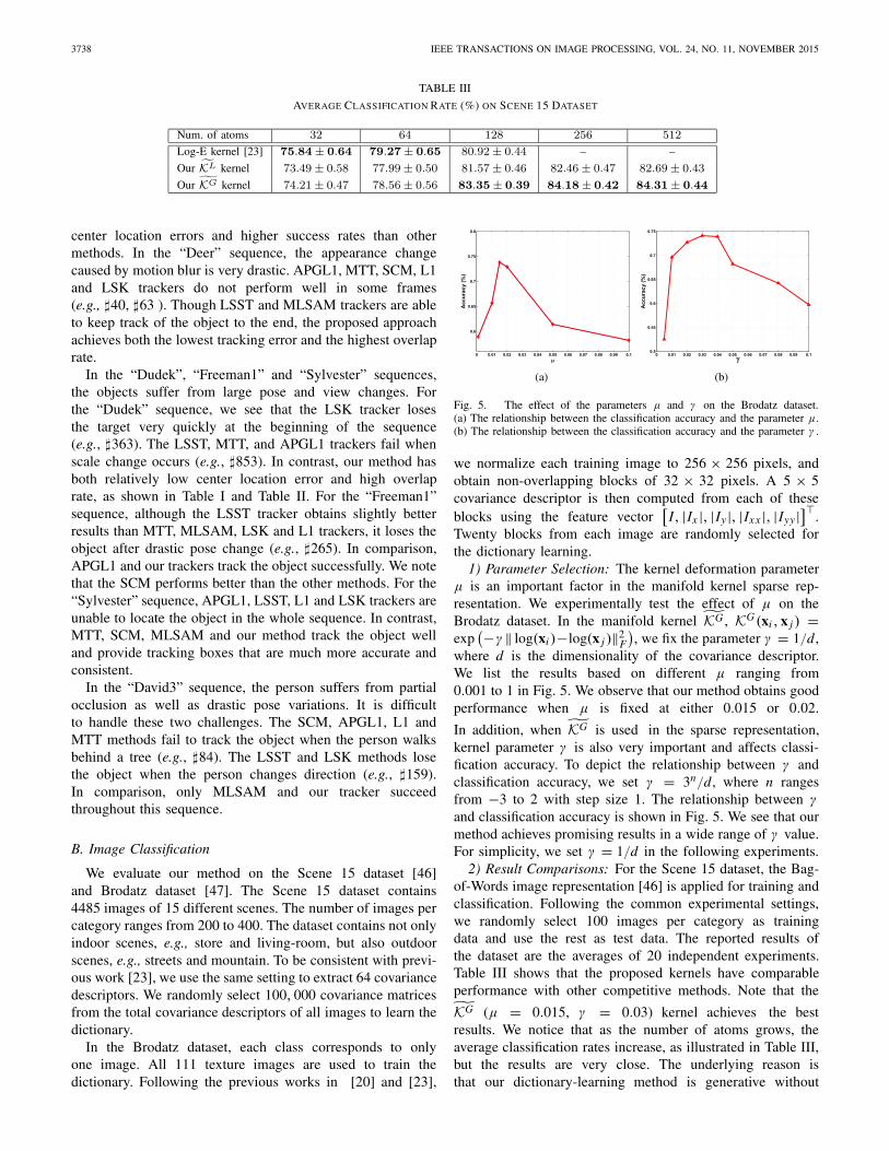
Fig. 5. The effect of the parameters μ and γ on the Brodatz dataset.(a) The relationship between the classification accuracy and the parameter μ.(b) The relationship between the classification accuracy and the parameter γ .

we normalize each training image to 256 × 256 pixels, andobtain non-overlapping blocks of 32 × 32 pixels. A 5 × 5covariance descriptor is then computed from each of theseblocks using the feature vector

[I, |Ix |, |Iy |, |Ix x |, |Iyy|

]�.Twenty blocks from each image are randomly selected forthe dictionary learning.

1) Parameter Selection: The kernel deformation parameterμ is an important factor in the manifold kernel sparse rep-resentation. We experimentally test the effect of μ on theBrodatz dataset. In the manifold kernel K̃G , KG (xi , x j ) =exp

(−γ ‖ log(xi )−log(x j )‖2F

), we fix the parameter γ = 1/d ,

where d is the dimensionality of the covariance descriptor.We list the results based on different μ ranging from0.001 to 1 in Fig. 5. We observe that our method obtains goodperformance when μ is fixed at either 0.015 or 0.02.

In addition, when K̃G is used in the sparse representation,kernel parameter γ is also very important and affects classi-fication accuracy. To depict the relationship between γ andclassification accuracy, we set γ = 3n/d , where n rangesfrom −3 to 2 with step size 1. The relationship between γand classification accuracy is shown in Fig. 5. We see that ourmethod achieves promising results in a wide range of γ value.For simplicity, we set γ = 1/d in the following experiments.

2) Result Comparisons: For the Scene 15 dataset, the Bag-of-Words image representation [46] is applied for training andclassification. Following the common experimental settings,we randomly select 100 images per category as trainingdata and use the rest as test data. The reported results ofthe dataset are the averages of 20 independent experiments.Table III shows that the proposed kernels have comparableperformance with other competitive methods. Note that the

K̃G (μ = 0.015, γ = 0.03) kernel achieves the bestresults. We notice that as the number of atoms grows, theaverage classification rates increase, as illustrated in Table III,but the results are very close. The underlying reason isthat our dictionary-learning method is generative without


TABLE IV

COMPARISON OF CLASSIFICATION ACCURACY (%)

ON THE BRODATZ DATASET

Fig. 6. The average classification accuracy curves vs. the number of atommatrices on the Brodatz dataset.

discriminative information, therefore, good representationalcapability does not necessarily signify promising discrim-inability.

We use the Brodatz dataset [47] to evaluate the performanceof our method on texture classification. We evaluate clas-sification performance with the number of training samplesfixed at 20, 25, and 30 covariance matrices per class, withthe remaining samples being used for testing. The reportedperformance is obtained by averaging over ten random splits oftraining and test sets. The KNN classifier is employed for theclassification task (k = 3). The results are reported in Table IV.It can be seen that our K̃L kernel (μ = 0.015) achievescomparable performance with the Log-Euclidean method [23].K̃G kernel (μ = 0.015, γ = 0.02) performs better thanother approaches, because the radial basis function K̃G betterreflects the geometrical structure of the manifold data than thepolynomial kernel K̃L . To further analyze our results, we plotthe average classification accuracy curves using K̃G versusthe number of atom matrices in Fig. 6. We see that as thenumber of atoms increases, the improvement of our methodgrows. Our method achieves the best result when the numberof atoms is equal to 95.

C. Face Recognition

In this section, we present experimental results for facerecognition on the FERET dataset [48] and the ExtendedYale B dataset [49]. The sparse representation classifier [4] isadopted for the classification task. We use the “b” subset of theFERET dataset for the evaluation of recognition performance.The subset includes 1400 images from 198 subjects. In ourexperiments, the images are resized to 64 × 64 pixels. TheExtended Yale B dataset contains about 2, 414 frontal faceimages of 38 subjects. The face images are taken undervarying illumination conditions. We normalize face images ofsize 54 × 48.

TABLE V

FACE RECOGNITION RATE (%) ON THE FERET DATASET

TABLE VI

COMPARISON OF THE AVERAGE RECOGNITION ACCURACY (%)

ON THE EXTENDED YALE B DATASET

1) Experimental Setup: To obtain the manifold kernelsparse representation, a 43 × 43 covariance descriptor is usedto describe a face image using the feature vector

[I (x, y), x, y, |G00(x, y)|, · · · , |G07(x, y)|, · · · ,

|G47(x, y)|]�,

where I (x, y) is the intensity value at position (x, y), andGuv (x, y) is the response of a 2D Gabor filter along fiveorientations and eight angles. For each pixel (x, y), the dimen-sionality of the Gabor features is 40. For the FERET dataset,images marked “ba”, “bj” and “bk” are used as training data,and images with “bd”, “be”, “bf” and “bg” labels are testdata. We randomly split the Extended Yale B dataset into twohalves. One half containing 32 images for each person is usedas the dictionary, and the other half is used for testing. On theExtended Yale B dataset, we conduct experiments 10 times byrandomly selecting training and testing sets, and we report theaverage result.

2) Result Comparisons: Table V shows the recognition rateson the FERET dataset compared with SRC [4], GSRC [5],TSC [12], RSR [20], and Log-E kernel [23]. We see thatneither SRC nor TSC is able to obtain satisfactory results,because the Riemannian manifold of Sym+

d lacks a globallinear structure which allows the SPD matrix to be generatedlinearly by the atoms in D. GSRC and RSR improve the recog-nition rates. Overall, the proposed method with K̃L achievescomparable performance with the Log-E kernel method, andK̃G (μ = 0.02, γ = 0.01) is slightly better than the Log-Ekernel method.

Table VI shows the recognition rates versus feature dimen-sion by SRC and GSRC on the Extended Yale B dataset.Since the Log-E kernel and our method acquire the covariancedescriptors which are independent of each image, it is notnecessary for these two methods to reduce the dimensionalityof the original face images. The results of both SRC andGSRC are from [5]. Our method with K̃G (μ = 0.02,γ = 0.015) achieves better results than the other methods,


but the K̃L kernel is slightly worse than SRC and GSRC whenthe dimension is 150.

VI. CONCLUSION

In this paper, we have presented a manifold kernel sparserepresentation method for symmetric positive definite (SPD)matrices. The sparse representation on the space of SPDmatrices can be performed by embedding the SPD matricesinto a reproducing kernel Hilbert space (RKHS) using thedata-dependent manifold kernel function. The graph Laplacianis incorporated into the manifold kernel space to discoverthe underlying geometrical structure of the manifold. Experi-mental results of visual tracking, face recognition and imageclassification show that our algorithm outperforms existingsparse coding based approaches, and compares favorably withstate-of-the-art methods.

ACKNOWLEDGEMENT

The authors would like to thank Zhen Dong andShiye Zhang for their efforts in conducting the experiments,and greatly appreciate Sue Felix polishing our presentation.Yuwei Wu thanks Mehrtash Harandi and Shengping Zhangfor the useful discussion on the revised version of our paper.

REFERENCES

[1] Z. Xiao, H. Lu, and D. Wang, “L2-RLS based object tracking,” IEEETrans. Circuits Syst. Video Technol., vol. 24, no. 8, pp. 1301–1309,Aug. 2014.

[2] T. Zhang, B. Ghanem, S. Liu, and N. Ahuja, “Robust visual trackingvia structured multi-task sparse learning,” Int. J. Comput. Vis., vol. 101,no. 2, pp. 367–383, 2013.

[3] Y. Wu, B. Ma, M. Yang, Y. Jia, and J. Zhang, “Metric learning basedstructural appearance model for robust visual tracking,” IEEE Trans.Circuits Syst. Video Technol., vol. 24, no. 5, pp. 865–877, May 2014.

[4] J. Wright, A. Y. Yang, A. Ganesh, S. S. Sastry, and Y. Ma, “Robust facerecognition via sparse representation,” IEEE Trans. Pattern Anal. Mach.Intell., vol. 31, no. 2, pp. 210–227, Feb. 2009.

[5] M. Yang and L. Zhang, “Gabor feature based sparse representation forface recognition with Gabor occlusion dictionary,” in Proc. Eur. Conf.Comput. Vis. (ECCV), 2010, pp. 448–461.

[6] S. Gao, I. W.-H. Tsang, and L.-T. Chia, “Laplacian sparse coding,hypergraph Laplacian sparse coding, and applications,” IEEE Trans.Pattern Anal. Mach. Intell., vol. 35, no. 1, pp. 92–104, Jan. 2013.

[7] M. Yang, L. Zhang, X. Feng, and D. Zhang, “Sparse representation basedFisher discrimination dictionary learning for image classification,” Int.J. Comput. Vis., vol. 109, no. 3, pp. 209–232, 2014.

[8] A. Cherian, S. Sra, A. Banerjee, and N. Papanikolopoulos,“Jensen–Bregman LogDet divergence with application to efficient simi-larity search for covariance matrices,” IEEE Trans. Pattern Anal. Mach.Intell., vol. 35, no. 9, pp. 2161–2174, Sep. 2013.

[9] S. Jayasumana, R. Hartley, M. Salzmann, H. Li, and M. Harandi, “Kernelmethods on the Riemannian manifold of symmetric positive definitematrices,” in Proc. IEEE Conf. Comput. Vis. Pattern Recognit. (CVPR),Jun. 2013, pp. 73–80.

[10] H. E. Cetingul and R. Vidal, “Intrinsic mean shift for clustering onStiefel and Grassmann manifolds,” in Proc. IEEE Conf. Comput. Vis.Pattern Recognit. (CVPR), Jun. 2009, pp. 1896–1902.

[11] M. Harandi, C. Sanderson, C. Shen, and B. Lovell, “Dictionary learningand sparse coding on Grassmann manifolds: An extrinsic solution,” inProc. IEEE Int. Conf. Comput. Vis. (ICCV), Dec. 2013, pp. 3120–3127.

[12] R. Sivalingam, D. Boley, V. Morellas, and N. Papanikolopoulos, “Tensorsparse coding for positive definite matrices,” IEEE Trans. Pattern Anal.Mach. Intell., vol. 36, no. 3, pp. 592–605, Mar. 2014.

[13] R. Sivalingam, D. Boley, V. Morellas, and N. Papanikolopoulos, “Posi-tive definite dictionary learning for region covariances,” in Proc. IEEEInt. Conf. Comput. Vis. (ICCV), Nov. 2011, pp. 1013–1019.

[14] S. Sra and A. Cherian, “Generalized dictionary learning for symmetricpositive definite matrices with application to nearest neighbor retrieval,”in Machine Learning and Knowledge Discovery in Databases. Berlin,Germany: Springer-Verlag, 2011, pp. 318–332.

[15] A. Cherian and S. Sra, “Riemannian sparse coding for positive definitematrices,” in Proc. Eur. Conf. Comput. Vis. (ECCV), 2014, pp. 299–314.

[16] M. Harandi, R. Hartley, B. Lovell, and C. Sanderson, “Sparsecoding on symmetric positive definite manifolds using Breg-man divergences,” IEEE Trans. Neural Netw. Learn. Syst., doi:10.1109/TNNLS.2014.2387383, 2015.

[17] X. Zhang, W. Li, W. Hu, H. Ling, and S. Maybank, “Block covariancebased �1 tracker with a subtle template dictionary,” Pattern Recognit.,vol. 46, no. 7, pp. 1750–1761, 2013.

[18] K. Guo, P. Ishwar, and J. Konrad, “Action recognition using sparserepresentation on covariance manifolds of optical flow,” in Proc. IEEEInt. Conf. Adv. Video Signal Based Surveill. (AVSS), Aug./Sep. 2010,pp. 188–195.

[19] C. Yuan, W. Hu, X. Li, S. Maybank, and G. Luo, “Human actionrecognition under Log-Euclidean Riemannian metric,” in Proc. AsianConf. Comput. Vis. (ACCV), 2010, pp. 343–353.

[20] M. T. Harandi, C. Sanderson, R. Hartley, and B. C. Lovell, “Sparsecoding and dictionary learning for symmetric positive definite matrices:A kernel approach,” in Proc. Eur. Conf. Comput. Vis. (ECCV), 2012,pp. 216–229.

[21] S. Zhang, S. Kasiviswanathan, P. C. Yuen, and M. Harandi, “Onlinedictionary learning on symmetric positive definite manifolds with visionapplications,” in Proc. AAAI Conf. Artif. Intell. (AAAI), 2015, pp. 1–9.

[22] A. Barachant, S. Bonnet, M. Congedo, and C. Jutten, “Classification ofcovariance matrices using a Riemannian-based kernel for BCI applica-tions,” Neurocomputing, vol. 112, pp. 172–178, Jul. 2013.

[23] P. Li, Q. Wang, W. Zuo, and L. Zhang, “Log-Euclidean kernels forsparse representation and dictionary learning,” in Proc. IEEE Int. Conf.Comput. Vis. (ICCV), Dec. 2013, pp. 1601–1608.

[24] R. Vemulapalli, J. K. Pillai, and R. Chellappa, “Kernel learningfor extrinsic classification of manifold features,” in Proc. IEEEConf. Comput. Vis. Pattern Recognit. (CVPR), Jun. 2013,pp. 1782–1789.

[25] V. Sindhwani, P. Niyogi, and M. Belkin, “Beyond the point cloud: Fromtransductive to semi-supervised learning,” in Proc. Int. Conf. Mach.Learn. (ICML), 2005, pp. 824–831.

[26] V. Arsigny, P. Fillard, X. Pennec, and N. Ayache, “Geometric means ina novel vector space structure on symmetric positive-definite matrices,”SIAM J. Matrix Anal. Appl., vol. 29, no. 1, pp. 328–347, 2006.

[27] O. Tuzel, F. Porikli, and P. Meer, “Pedestrian detection via classificationon Riemannian manifolds,” IEEE Trans. Pattern Anal. Mach. Intell.,vol. 30, no. 10, pp. 1713–1727, Oct. 2008.

[28] Y. Pang, Y. Yuan, and X. Li, “Gabor-based region covariance matricesfor face recognition,” IEEE Trans. Circuits Syst. Video Technol., vol. 18,no. 7, pp. 989–993, Jul. 2008.

[29] J. Y. Tou, Y. H. Tay, and P. Y. Lau, “Gabor filters as feature imagesfor covariance matrix on texture classification problem,” in Advances inNeuro-Information Processing. Berlin, Germany: Springer-Verlag, 2009,pp. 745–751.

[30] J. Mairal, F. Bach, J. Ponce, and G. Sapiro, “Online learning formatrix factorization and sparse coding,” J. Mach. Learn. Res., vol. 11,pp. 19–60, Mar. 2010.

[31] H. V. Nguyen, V. M. Patel, N. M. Nasrabadi, and R. Chellappa, “Kerneldictionary learning,” in Proc. IEEE Int. Conf. Acoust., Speech SignalProcess. (ICASSP), Mar. 2012, pp. 2021–2024.

[32] H. Van Nguyen, V. M. Patel, N. M. Nasrabadi, and R. Chellappa,“Design of non-linear kernel dictionaries for object recognition,” IEEETrans. Image Process., vol. 22, no. 12, pp. 5123–5135, Dec. 2013.

[33] S. Gao, I. W.-H. Tsang, and L.-T. Chia, “Sparse representation withkernels,” IEEE Trans. Image Process., vol. 22, no. 2, pp. 423–434,Feb. 2013.

[34] J. J. Thiagarajan, K. N. Ramamurthy, and A. Spanias, “Multiple kernelsparse representations for supervised and unsupervised learning,” IEEETrans. Image Process., vol. 23, no. 7, pp. 2905–2915, Jul. 2014.

[35] M. J. Gangeh, A. Ghodsi, and M. S. Kamel, “Kernelized superviseddictionary learning,” IEEE Trans. Signal Process., vol. 61, no. 19,pp. 4753–4767, Oct. 2013.

[36] F. R. K. Chung, Spectral Graph Theory, vol. 92. Providence, RI,USA: AMS, 1997.

[37] S. C. H. Hoi, R. Jin, J. Zhu, and M. R. Lyu, “Semi-supervised SVMbatch mode active learning for image retrieval,” in Proc. IEEE Conf.Comput. Vis. Pattern Recognit. (CVPR), Jun. 2008, pp. 1–7.


[38] C. van den Berg, J. P. R. Christensen, and P. Ressel, Harmonic Analysison Semigroups: Theory of Positive Definite and Related Functions.New York, NY, USA: Springer-Verlag, 1984.

[39] R. Tibshirani, “Regression shrinkage and selection via the lasso,” J. Roy.Statist. Soc. B (Methodological), vol. 58, no. 1, pp. 267–288, 1996.

[40] W. Zhong, H. Lu, and M.-H. Yang, “Robust object tracking via sparsecollaborative appearance model,” IEEE Trans. Image Process., vol. 23,no. 5, pp. 2356–2368, May 2014.

[41] D. Wang, H. Lu, and M.-H. Yang, “Least soft-threshold squares track-ing,” in Proc. IEEE Conf. Comput. Vis. Pattern Recognit. (CVPR),Jun. 2013, pp. 2371–2378.

[42] B. Liu, J. Huang, C. Kulikowski, and L. Yang, “Robust visual trackingusing local sparse appearance model and K-selection,” IEEE Trans.Pattern Anal. Mach. Intell., vol. 35, no. 12, pp. 2968–2981, Dec. 2013.

[43] N. Xie, H. Ling, W. Hu, and X. Zhang, “Use bin-ratio information forcategory and scene classification,” in Proc. IEEE Conf. Comput. Vis.Pattern Recognit. (CVPR), Jun. 2010, pp. 2313–2319.

[44] X. Mei and H. Ling, “Robust visual tracking using �1 minimization,”in Proc. IEEE 12th Int. Conf. Comput. Vis. (ICCV), Sep./Oct. 2009,pp. 1436–1443.

[45] C. Bao, Y. Wu, H. Ling, and H. Ji, “Real time robust L1 tracker usingaccelerated proximal gradient approach,” in Proc. IEEE Conf. Comput.Vis. Pattern Recognit. (CVPR), Jun. 2012, pp. 1830–1837.

[46] S. Lazebnik, C. Schmid, and J. Ponce, “Beyond bags of features: Spatialpyramid matching for recognizing natural scene categories,” in Proc.IEEE Conf. Comput. Vis. Pattern Recognit. (CVPR), vol. 2. Jun. 2006,pp. 2169–2178.

[47] T. Randen and J. H. Husoy, “Filtering for texture classification: A com-parative study,” IEEE Trans. Pattern Anal. Mach. Intell., vol. 21, no. 4,pp. 291–310, Apr. 1999.

[48] P. J. Phillips, H. Moon, S. A. Rizvi, and P. J. Rauss, “The FERETevaluation methodology for face-recognition algorithms,” IEEE Trans.Pattern Anal. Mach. Intell., vol. 22, no. 10, pp. 1090–1104, Oct. 2000.

[49] K.-C. Lee, J. Ho, and D. Kriegman, “Acquiring linear subspaces for facerecognition under variable lighting,” IEEE Trans. Pattern Anal. Mach.Intell., vol. 27, no. 5, pp. 684–698, May 2005.

Yuwei Wu received the Ph.D. degree in computerscience from the Beijing Institute of Technology,Beijing, China, in 2014. He is currently a ResearchFellow with the School of Electrical and Elec-tronic Engineering, Nanyang Technological Univer-sity, Singapore. He has strong research interestsin computer vision, medical image processing, andobject tracking. He received a National Scholarshipfor Graduate Students and an Academic Scholarshipfor Ph.D. Candidates from the Ministry of Educa-tion, China, an Outstanding Ph.D. Thesis Award and

XU TELI Excellent Scholarship from the Beijing Institute of Technology,and a CASC Scholarship from the China Aerospace Science and IndustryCorporation.

Yunde Jia (M’11) received the B.S., M.S., andPh.D. degrees in mechatronics from the BeijingInstitute of Technology (BIT), in 1983, 1986, and2000, respectively. He was a Visiting Scientist withCarnegie Mellon University from 1995 to 1997,and a Visiting Fellow with the Australian NationalUniversity in 2011. He has served as the ExecutiveDean of the School of Computer Science at BITfrom 2005 to 2008. He is currently a Professor ofComputer Science at BIT, and serves as the Directorof the Beijing Laboratory of Intelligent Information

Technology. His current research interests include computer vision, mediacomputing, and intelligent systems.

Peihua Li received the B.S. and M.S. degrees fromthe Harbin Engineering University, China, in 1993and 1996, respectively, and the Ph.D. degree incomputer science and technology from the HarbinInstitute of Technology, China, in 2002. In 2003, hevisited Microsoft Research Asia. From 2003 to 2004,he was a Post-Doctoral Fellow at INRIA, IRISA,Rennes, France. From 2004 to 2013, he was with theSchool of Computer Science and Technology, Hei-longjiang University. He is currently with the Schoolof Information and Communication Engineering,

Dalian University of Technology. His research interests include computervision, pattern recognition, and machine learning. He received the Best Ph.D.Dissertation Award from the Harbin Institute of Technology, in 2004, andhonorary nomination for the National Excellent Doctoral Dissertation Awardin China in 2005.

Jian Zhang (SM’04) received the B.Sc. degree fromEast China Normal University, Shanghai, China, in1982, the M.Sc. degree in computer science fromFlinders University, Adelaide, Australia, in 1994,and the Ph.D. degree in electrical engineering fromthe University of New South Wales (UNSW),Sydney, Australia, in 1999.

He was with the Visual Information ProcessingLaboratory, Motorola Laboratories, Sydney, from1997 to 2003, as a Senior Research Engineer, andlater became a Principal Research Engineer and a

Foundation Manager with the Visual Communications Research Team. From2004 to 2011, he was a Principal Researcher and a Project Leader withNational ICT Australia, Sydney, and a Conjoint Associate Professor withthe School of Computer Science and Engineering, UNSW. He is currentlyan Associate Professor with the Advanced Analytics Institute, School ofSoftware, Faculty of Engineering and Information Technology, University ofTechnology at Sydney, Sydney, and a Visiting Researcher with the NevilleRoach Laboratory, National ICT Australia, Kensington, Australia. He is theauthor or co-author of more than 100 paper publications, book chapters, andsix issued patents filed in the U.S. and China. His current research interestsinclude social multimedia signal processing, image and video processing,machine learning, pattern recognition, human–computer interaction, and intel-ligent healthcare systems.

Dr. Zhang was the General Chair of the IEEE International Conference onMultimedia and Expo in 2012. He is also an Associate Editor of the IEEETRANSACTIONS ON CIRCUITS AND SYSTEMS FOR VIDEO TECHNOLOGYand the EURASIP Journal on Image and Video Processing.

Junsong Yuan (M’08) received the Ph.D. degreefrom Northwestern University, USA, and theM.Eng. degree from the National University ofSingapore. He graduated from the Special Classfor the Gifted Young of the Huazhong Universityof Science and Technology, China. He is currentlyan Assistant Professor and a Program Directorof Video Analytics with the School of Electricaland Electronic Engineering, Nanyang TechnologicalUniversity, Singapore. He is the author or co-authorof more than100 paper publications, book chapters,

and six issued patents filed in the U.S. and China. His research interestsinclude computer vision, video analytics, large-scale visual search and mining,and human–computer interaction.

He has served as the Area Chair of the IEEE Winter Conference onComputer Vision, the IEEE Conference on Multimedia Expo (ICME) in2014, and the Asian Conference on Computer Vision (ACCV) in 2014, theOrganizing Chair of ACCV in 2014, and the Co-Chair Workshops at the IEEEConference on Computer Vision and Pattern Recognition (CVPR 12, 13)and the IEEE Conference on Computer Vision. He currently serves as anAssociate Editor of The Visual Computer journal (TVC) and the Journalof Multimedia. He received the Nanyang Assistant Professorship and TanChin Tuan Exchange Fellowship from Nanyang Technological University, anOutstanding EECS Ph.D. Thesis Award from Northwestern University, theBest Doctoral Spotlight Award from CVPR 09, and the National OutstandingStudent from the Ministry of Education, China. He has recently given tutorialsat the IEEE ICIP13, FG13, ICME12, SIGGRAPH VRCAI12, and PCM12.

ieee transactions on image processing, vol. 24, no. 11 ...jsyuan/papers/2015... · matrices, visual...

Documents