ieee transactions on image processing 1 …ybchen/tip2017watermark.pdf · ieee proof ieee...

IEEE P

roof

IEEE TRANSACTIONS ON IMAGE PROCESSING 1

Robust Multi-Focus Image Fusion UsingEdge Model and Multi-Matting

Yibo Chen , Member, IEEE, Jingwei Guan , Member, IEEE, and Wai-Kuen Cham, Senior Member, IEEE

Abstract— An effective multi-focus image fusion method is1

proposed to generate an all-in-focus image with all objects in2

focus by merging multiple images. The proposed method first3

estimates focus maps using a novel combination of edge model4

and a traditional block-based focus measure. Then, a propagation5

process is conducted to obtain accurate weight maps based on a6

novel multi-matting model that makes full use of the spatial infor-7

mation. The fused all-in-focus image is finally generated based8

on a weighted-sum strategy. Experimental results demonstrate9

that the proposed method has state-of-the-art performance for10

multi-focus image fusion under various situations encountered in11

practice, even in cases with obvious misregistration.12

Index Terms— Multi-focus, fusion, edge model, multi-matting.13

I. INTRODUCTION14

MULTI-FOCUS image fusion is an important technique15

to tackle the defocus problem that some parts of the16

image are out of focus and look blurry. This problem usually17

happens when a low depth-of-field optical system is used18

to capture an image, such as microscopes or large aperture19

cameras. Through multi-focus image fusion, several images20

of the same scene but with different focus settings can be21

combined into a so-called all-in-focus image, in which all22

parts are fully focused. A good multi-focus image fusion23

method should meet the requirements that all information24

of the focused regions in each source image is preserved25

in the fused image with little artifacts, and the method is26

robust to imperfect situations such as existence of noise and27

misregistration.28

During the last decade, a large number of multi-focus image29

fusion methods have been proposed. Most of them can be30

categorized into four major groups [1]. The first group consists31

of methods based on multi-scale decomposition [2], such as32

pyramid [3], wavelet decomposition [4], [5], curvelet trans-33

form [6], shearlet transform [7], non-subsampled contourlet34

transform (NSCT) [8], [9] and neighbor distance (ND) [10].35

Recently guided filter was also introduced to refine the multi-36

scale representations and the method achieves state-of-the-37

art performance [11]. The second group consists of sparse38

Manuscript received January 10, 2017; revised June 29, 2017; acceptedNovember 20, 2017. The associate editor coordinating the review of thismanuscript and approving it for publication was Prof. Gene Cheung.(Corresponding author: Yibo Chen.)

The authors are with the Department of Electrical Engineering, The ChineseUniversity of Hong Kong, Hong Kong (e-mail: [email protected];[email protected]; [email protected]).

Color versions of one or more of the figures in this paper are availableonline at http://ieeexplore.ieee.org.

Digital Object Identifier 10.1109/TIP.2017.2779274

representation (SR) based methods. The concept of SR was 39

first introduced into image fusion in [12], which employs the 40

orthogonal matching pursuit algorithm to image patches of 41

multiple source images. Adaptive SR model was proposed 42

in [13] for simultaneous image fusion and denoising. In [14], 43

an over-complete dictionary was learned from numerous 44

training samples similar to the source images, thus adding 45

adaptability for the sparse representation. Zhang et al. [15] 46

also proposed a multi-task SR method that considers not 47

only sharpness information, like edges and textures, of each 48

image patch but also relationship among source images. The 49

major advantage of these two groups of methods is that 50

sharpness information can be well preserved in the fused 51

image. However, since spatial consistency is not fully con- 52

sidered, brightness and color distortions may be observed. 53

Moreover, slight image misregistration will result in ghosting 54

artifacts due to their sensitivity to high-frequency components. 55

The third group consists of methods based on computational 56

photography techniques such as light field rendering [16]. This 57

kind of methods discovers more of the physical formation of 58

multi-focus images and reconstructs the all-in-focus images. 59

The last group consists of methods performed in spatial 60

domain, which can make full use of the spatial context and 61

provide spatial consistency. A commonly used approach is to 62

take each pixel in the fused image as the weighted average 63

of the corresponding pixels in the source images. The weights 64

are determined according to how well each pixel is focused, 65

which is usually measured by some metrics. These metrics, 66

such as spatial frequency inside a surrounding block, are 67

named as focus measures. However, this kind of methods 68

may generate blocking artifacts on object boundaries due 69

to the block-based computation of focus measure. To solve 70

this problem, some region-based fusion methods have been 71

proposed and calculation is done in regions with irregular 72

shapes obtained by segmentation [17]. A common limitation of 73

region-based methods is that they rely heavily on the accuracy 74

of segmentation. Another way is post-processing of the initial 75

weight maps [18]–[20]. In [21], a noise-robust selective fusion 76

method that models the change of weights as a Gaussian 77

function is proposed, but it can only achieve good perfor- 78

mance on properly ordered image sequence with 3 or more 79

images. Recently, image matting was introduced to refine the 80

initial weight maps and can achieve good performance [22]. 81

However, the performance relies on good initial weight maps, 82

and the common block-wise computation is still a limitation. 83

Our previous work [23] uses one of the parameters of edge 84

model directly as focus measure. However, edge model is a 85

1057-7149 © 2017 IEEE. Personal use is permitted, but republication/redistribution requires IEEE permission.See http://www.ieee.org/publications_standards/publications/rights/index.html for more information.

https://orcid.org/0000-0002-6632-6359

https://orcid.org/0000-0001-7346-5317

IEEE P

roof

2 IEEE TRANSACTIONS ON IMAGE PROCESSING

sparse feature representation method and focus measure values86

only exist at edge locations. So image matting was applied to87

propagate the focus measure values to the whole image. Since88

the matting process handles source images separately without89

considering the correlation among them, the propagation effect90

is very limited and the fusion process is also not stable in many91

situations.92

To solve the problems mentioned above, a novel edge model93

and multi-matting (EMAM) based multi-focus image fusion94

method is proposed in this paper, which can be classified as the95

fourth group of methods. Firstly, a novel method that combines96

a traditional focus measure and edge model is developed97

to estimate focus maps. Then a new multi-matting model98

is proposed to spread the focus maps to the whole image99

region considering the correlation among source images and100

obtain final weight maps. The proposed method maintains the101

advantages of the last group of methods and meanwhile over-102

comes the weakness. Experimental results demonstrate that the103

proposed method outperforms current state-of-the-art fusion104

methods under various situations. The main contributions of105

the proposed fusion approach are highlighted as follows.106

(i) The utilization of edge model when estimating focus107

maps removes block artifacts but allows sharpness information108

to be preserved as good as the first two groups of methods.109

The combination of edge model with traditional focus measure110

makes the proposed method robust to noise.111

(ii) The proposed multi-matting model makes full use of the112

spatial consistency and the correlation among source images,113

and thus achieves better performance at object boundaries than114

region-based methods and existing matting-based methods.115

The multi-matting scheme also produces improved robustness116

to misregistration.117

The rest of the paper is organized as follows. A brief118

introduction of the defocus model and edge model is given in119

section II. Section III gives problem formulation and details120

the proposed image fusion algorithm. Experimental results121

and conclusions are presented in Section IV and Section V122

respectively.123

II. BACKGROUND124

A. Defocus Model125

When a scene is captured using a camera, a surface which is126

not on the focal plane will form a blur region on the image, and127

the region is regarded as defocused. Such blurring process is128

usually modeled as a 2D linear space-invariant system, which129

is characterized as the convolution of the ideal focused content130

in that region f (x, y) with a space-invariant Point Spread131

Function (PSF) h(x, y):132

g(x, y) = h(x, y) ⊗ f (x, y) + n(x, y), (1)133

where g(x, y) denotes the defocused content, n(x, y) is noise134

and ⊗ denotes convolution operator. In practice, due to the135

polychromatic illumination, diffraction, camera lens aberra-136

tion, etc., the PSF is usually approximated by a 2D Gaussian137

filter [24], [25], that is:138

h(x, y; σ f ) = 1

2πσ 2f

ex p(− x2 + y2

2σ 2f

), (2)139

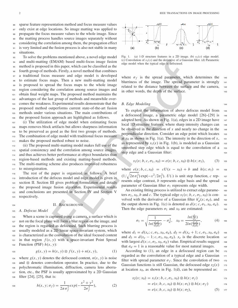
Fig. 1. (a) 1-D structure features in a 2D image. (b) s1(x) edge model.(c) Convolution of s1(x) and the derivative of a Gaussian filter. (d) Parametricedge model when the typical edge is defocused.

where σ f is the spread parameter, which determines the 140

blurriness of the image. The spread parameter is strongly 141

related to the distance between the surface and the camera, 142

in other words, the depth of the surface. 143

B. Edge Modeling 144

To exploit the information of above defocus model from 145

a defocused image, a parametric edge model [26]–[29] is 146

adopted here. As shown in Fig. 1(a), edges in a 2D image have 147

local 1D structure features, where sharp intensity changes can 148

be observed in the direction of x and nearly no change in the 149

perpendicular direction. Consider an edge point which locates 150

at x0 as shown in Fig. 1(a). The intensity in the direction of x , 151

as represented by s1(x) in Fig. 1(b), is modeled as a Gaussian 152

smoothed step edge which is equal to the convolution of a 153

step edge and a Gaussian filter: 154

s1(x; b, c, σ1, x0) = e(x; b, c, x0) ⊗ h(x; σ1), (3) 155

where e(x; b, c, x0) = cU(x − x0) + b and h(x; σ1) = 156

(1/√

2πσ 21 ) exp(−x2/2σ 2

1 ). U(·) is unit step function, c rep- 157

resents edge contrast, b represents edge basis and the spread 158

parameter of Gaussian filter σ1 represents edge width. 159

An existing fitting process is utilized to extract edge parame- 160

ters σ1, x0, b and c. The typical edge s1(x; b, c, σ1, x0) is con- 161

volved with the derivative of a Gaussian filter h′d(x; σd), and 162

the output shown in Fig. 1(c) is denoted as d(x; c, σ1, x0, σd ). 163

Then the edge parameters σ1 and x0 are estimated: 164

σ1 =√

1

ln( d1d1d2d3

)− σ 2

d , x0 = ln( d2d3

)

2ln( d1d1d2d3

), (4) 165

where d1 = d(xe; c, σ1, x0, σd ), d2 = d(xe + 1; c, σ1, x0, σd ) 166

and d3 = d(xe − 1; c, σ1, x0, σd ). xe is the discrete location 167

with largest d(x; c, σ1, x0, σd ) value. Empirical results suggest 168

that σd = 1 is a reasonable value for most natural images. 169

According to (1), an edge in a defocused region can be 170

regarded as the convolution of a typical edge and a Gaussian 171

filter with spread parameter σ f . Since the convolution of two 172

Gaussian functions is still Gaussian, the defocused edge s2(x) 173

at location x0, as shown in Fig. 1(d), can be represented as: 174

s2(x; x0) = s1(x; b, c, σ1, x0) ⊗ h(x; σ f ) 175

= e(x; b, c, x0) ⊗ h(x; σ1) ⊗ h(x; σ f ) 176

= e(x; b, c, x0) ⊗ h(x; σ2), (5) 177

IEEE P

roof

CHEN et al.: ROBUST MULTI-FOCUS IMAGE FUSION USING EDGE MODEL AND MULTI-MATTING 3

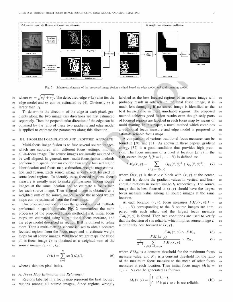
Fig. 2. Schematic diagram of the proposed image fusion method based on edge model and multi-matting model.

where σ2 =√

σ 21 + σ 2

f . The defocused edge s2(x) also fits the178

edge model and σ2 can be estimated by (4). Obviously σ2 is179

larger than σ1.180

To determine the direction of the edge at each pixel, gra-181

dients along the two image axis directions are first estimated182

separately. Then the perpendicular direction of the edge can be183

obtained by the ratio of these two gradients and edge model184

is applied to estimate the parameters along this direction.185

III. PROBLEM FORMULATION AND PROPOSED APPROACH186

Multi-focus image fusion is to fuse several source images,187

which are captured with different focus settings, into an188

all-in-focus image. The source images are usually assumed to189

be well aligned. In general, most multi-focus fusion methods190

performed in spatial domain contain two steps: focused region191

identification and focus map estimation, weight map estima-192

tion and fusion. Each source image is only well focused in193

some local regions. To identify these focused regions, focus194

measure is usually used to make comparisons among source195

images at the same location and to estimate a focus map196

for each source image. Then a fused image is obtained as a197

weighted sum of the source images, where the needed weight198

maps can be estimated from the focus maps.199

Our proposed method follows the general steps of methods200

performed in spatial domain. Fig. 2 summarizes the main201

processes of the proposed fusion method. First, initial focus202

maps are estimated using a traditional focus measure, and203

the edge model described in section II-B is utilized to refine204

them. Then a multi-matting scheme is used to obtain accurate205

focused regions from the focus maps and to estimate weight206

maps for all source images. With these weight maps, the fused207

all-in-focus image IF is obtained as a weighted sum of the208

source images I1, · · · , IN :209

IF (i) =N∑

k=1

wk(i)Ik(i), (6)210

where i denotes pixel index.211

A. Focus Map Estimation and Refinement212

Regions labelled in a focus map represent the best focused213

regions among all source images. Since regions wrongly214

labelled as the best focused regions of an source image will 215

probably result in artifacts in the final fused image, it is 216

much less damaging if no source image is identified as the 217

best focused one in these unreliable regions. The proposed 218

method achieves good fusion results even though only parts 219

of focused regions are labelled in each focus map by means of 220

multi-matting. In this paper, a novel method which combines 221

a traditional focus measure and edge model is proposed to 222

estimate reliable focus maps. 223

A comparison of various traditional focus measures can be 224

found in [30] and [31]. As shown in these papers, gradient 225

energy [32] is a good candidate that provides high preci- 226

sion. The focus measure of a pixel at location (x, y) in the 227

k-th source image Ik(k = 1, · · · , N) is defined as: 228

F Mk(x, y) =∑

(x,y)∈�(x,y)

(Ikx (x, y)2 + Iky(x, y)2), (7) 229

where �(x, y) is the r × r block with (x, y) at the center, 230

Ikx and Iky denote the gradient values in vertical and hori- 231

zontal directions in source image Ik respectively. The source 232

image that is best focused at (x, y) should have the largest 233

focus measure value among all source images at the same 234

location. 235

At each location (x, y), focus measures F Mk(x, y)(k = 236

1, · · · , N) corresponding to the N source images are com- 237

pared with each other, and the largest focus measure 238

F Mt (x, y) is found. Then two conditions are used to verify 239

that the decision of t is reliable, which implies source image It 240

is definitely best focused at (x, y). 241

F Mt (x, y) > F Mth, (8) 242

F Mt (x, y)1

N−1

∑k �=t,k=1,··· ,N

F Mk(x, y)> Rth, (9) 243

where F Mth is a constant threshold for the maximum focus 244

measure value, and Rth is a constant threshold for the ratio 245

of the maximum focus measure to the mean of other focus 246

measures at each location. Then initial focus maps Mk(k = 247

1, · · · , N) can be generated as follows. 248

Mk(x, y) ={

1 if k = t,

0 if k �= t or t is not reliable.(10) 249

IEEE P

roof


Fig. 3. Comparison between the blocks at the same position of two sourceimages. (a) Source image 1 and extracted block. (b) Source image 2 andextracted block. Point A′ has higher focus measure value than A, but point Bhas higher focus measure value than B ′ due to block computation.

Fig. 4. Initial focus maps of the two source images. (a) Focus map of sourceimage 1 and extracted block. (b) Focus map of source image 2 and extractedblock.

It should be noted that at some locations no source image250

satisfies conditions (8) and (9). Thus, the decision of t is251

regarded as not reliable and all focus maps will be set to252

zeros at these locations. One reason for these two conditions is253

based on observations of wrong decisions in flat regions which254

have little texture. For each location in these regions, the focus255

measures of source images generally have low magnitude and256

low inter-image contrast. The decision of t will be unstable257

and therefore (8) and (9) are introduced.258

Another reason is the limitation of block computation,259

which is demonstrated in Fig. 3. Source image 1 in Fig. 3a260

focuses in background (a big clock) and source image 2 in261

Fig. 3b focuses in foreground (a small clock). Since focus262

measure of each pixel is computed from all gradients inside263

an r × r block centered at the pixel, problems may arise at264

the boundary of foreground and background. This is especially265

true when the block centered at a pixel contains both rich fore-266

ground texture and rich background texture, such as pixel B267

and pixel B ′ in Fig. 3. B and B ′ are actually foreground pixels268

and the focus measure of B ′ should be larger than that of B269

since B ′ is better focused. But the sharp edges of shape ‘8’ in270

the background, which are inside the block centered at B ,271

greatly influence the computation of focus measure. Thus,272

the focus measure of B ′ may be very similar to B , which273

will make the comparison result unreliable. This problem does274

not happen for pixels A and A′, which are also at a same275

location, since the background inside the block centered at that276

location is flat with little texture and will not influence focus277

measure computation. Fig. 4 shows the initial focus maps of278

the two source images from Fig. 3, where only reliable pixels279

such as A are marked and confusing pixels such as B will be280

ignored by conditions (8) and (9).281

However, these confusing pixels carry important infor-282

mation which can be used as a guidance at the boundary283

of foreground and background, and it is unwise to simply284

Fig. 5. Refined focus maps using edge model. (a) Focus map of sourceimage 1 and extracted block. (b) Focus map of source image 2 and extractedblock.

ignore them. That is why edge model is introduced. Since 285

edge width σ and edge location x0 are calculated using only a 286

few nearby pixels instead of a block, as stated in Section II-B, 287

they represent the edges at the boundary more precisely and 288

complement the ignored information. However, estimation 289

of edge model parameters may not be accurate in regions 290

where edges are too serried and irregular, in which case the 291

gradient energy focus measure performs better. Besides, direct 292

comparison of edge width σ is sensitive to the location shift 293

of edges among source images, especially when the source 294

images are not perfectly aligned. Therefore edge model and the 295

gradient energy focus measure are combined to complement 296

each other by following steps. 297

Firstly, edge width σ and edge location x0 are calculated 298

for each pixel based on (4). Then an edge map for each source 299

image is obtained with values of edge width at corresponding 300

edge locations. However, estimation of edge location x0 will 301

be inaccurate when edge is heavily defocused. In other words, 302

edge locations calculated from edges with large edge width 303

values are not reliable. It is shown in [26] that for most 304

well-captured natural images, clear edges have edge width σ 305

ranging from 0.01 to 0.5. Thus for each edge map, only edge 306

locations with edge width smaller than σth = 0.5 are remained. 307

Secondly, an edge linking algorithm [33] is applied to refine 308

the edge maps and all connected edge contours in each edge 309

map are listed. Finally, for each edge contour, we identify the 310

source image in which this contour is more likely to be focused 311

and the whole edge contour will be added to corresponding 312

focus map. The values of initial focus map Mk along this edge 313

contour are summed up to give a score of source image Ik , 314

and the source image with the largest score is regarded as the 315

best focused one for this contour. Then refined focus maps are 316

obtained, which are shown in Fig. 5. If the focus maps have 317

some intersections, though only at very few locations, we will 318

eliminate these locations from all focus maps to ensure the 319

focus maps reliable. Edge model gives an instruction in those 320

confusing regions, refines the initial focus maps, and greatly 321

benefits the following multi-matting process. 322

Edge model is used instead of Canny edge detector because 323

edge model provides parameter σ in addition to edge contour. 324

Information of σ plays an important role in the proposed 325

algorithm and cannot be replaced by the threshold of Canny 326

edge detector. As described in Section II, defocus process 327

is modeled as Gaussian blur. Edge model is derived from 328

this defocus model and parameter σ perfectly represents the 329

degree of defocus, uninfluenced by edge contrast. However, 330

Canny edge detector uses gradient as measure, which is easily 331

IEEE P

roof


influenced by edge contrast, and setting a threshold for Canny332

edge’s measure is not accurate when examining the degree of333

defocus. Thus, the edge map produced by edge model is more334

reliable and fit for our purpose.335

B. Weight Map Estimation With Multi-Matting336

Model and Fusion337

Since only parts of focused regions are labelled in each338

focus map after the above focus map estimation, a propagation339

step is needed to spread them based on local smoothness340

assumptions of colors. Then weight maps are obtained and341

used to generate the fused all-in-focus image. Image matting342

algorithm is a good choice which is adapted to meet our343

demand.344

1) Image Matting and Application in Multi-Focus Fusion:345

Image matting aims at extracting foreground and background346

from an observed image Io. Foreground and background will347

be represented as layers Ip1 and Ip2 respectively. The color348

of i -th pixel in Io is assumed to be a linear combination of349

the colors in the two layers350

Io(i) = α(i)Ip1(i) + (1 − α(i))Ip2(i), (11)351

where α is the opacity of layer Ip1 called alpha matte.352

α(i) = 1 or 0 means the i -th pixel belongs to layer Ip1 or353

layer Ip2, respectively. Image matting is to obtain an accurate354

alpha matte α together with the two layers. Since solving the355

three unknowns α, Ip1, Ip2 in (11) from a single image Io is an356

underconstrained problem, additional information is required357

to extract a good matte. Most recent methods [34]–[36] use a358

trimap which roughly segments the image into three regions:359

layer Ip1, layer Ip2 and unknown.360

Among all image matting algorithms, the closed-form mat-361

ting method by Levin [36] is a good choice because of its362

high accuracy and low requirement of trimap. This method is363

based on local smoothness assumptions on colors of the two364

layers, which also stand for the case of focus map. The alpha365

matte is obtained by solving366

arg minα

αT Lα + λ(αT − αTs )Ds(α − αs), (12)367

where αs is the vector form of the trimap and Ds is a diagonal368

matrix whose diagonal elements are one for labelled pixels369

which have specified alpha values in the trimap and zero for370

all the other pixels. λ is a parameter that controls the similarity371

between alpha matte α and the trimap αs at labelled locations.372

Usually λ is a large number to keep them consistent at labelled373

locations. For a color image, L is a matting Laplacian matrix374

whose (i, j)th element is375

∑

p|(i, j )∈Tp

(δi j − 1

Np

(1 + (I (i) − μp)(Cp + ε

NpE3)

−1376

(I ( j) − μp)))

, (13)377

where δi j is the Kronecker delta function, I (i) is the i -th378

pixel of image I and I ( j) is the j -th pixel of image I . The379

summation is done for all windows Tp that contain these two380

pixels. Tp is the 3 × 3 window centered at p-th pixel, Np is381

the number of pixels in this window, μp and Cp are the mean 382

vector and covariance matrix of this window respectively. E3 is 383

the 3 × 3 identity matrix and ε is a regularizing parameter. 384

Since the cost function (12) is quadratic, α is obtained by 385

solving the following sparse linear system: 386

(L + λDs)α = λDsαs . (14) 387

Image matting algorithms can be used to obtain accurate 388

focused region in image and video applications [37], [38]. 389

More specifically, for each source image, regions which 390

are best focused among all source images are regarded as 391

layer Ip1, and the remaining regions are all regarded as 392

layer Ip2. The refined focus map obtained in Section III-A 393

can be used as the trimap. The resulting alpha matte obtained 394

by the matting algorithm above can discriminate needed best 395

focused regions from each source image, and the alpha matte 396

is regarded as an initial weight map. 397

However, this image matting method can only handle a 398

single image at one time. In the case of multi-focus fusion, 399

two or more focus maps need to be handled, each of which 400

corresponds to one of the source images. A common idea is to 401

separately handle each focus map using the abovementioned 402

single image matting and then normalize the generated initial 403

weight maps to make them sum up to one at each location. 404

Then these normalized weight maps are used to obtain multi- 405

focus fusion result by the weighted sum of source images. 406

However, this idea has problems when all initial weight maps 407

have very small values at some locations. Errors will be 408

magnified at these locations and the fusion result will not be 409

stable. Besides, source images are actually capturing the same 410

scene and must have high correlation, which is also not fully 411

utilized. Another similar method can be found in [22], which 412

uses single image matting to obtain initial weight maps and 413

generates final weight maps using a non-linear combination 414

of these initial weight maps. However, source images are not 415

treated with equal importance under the non-linear operation, 416

and different order of source images will lead to different 417

fusion result. Besides, one of the focus maps is not used in 418

the non-linear operation, which will cause information lost and 419

errors possibly. Moreover, it cannot solve the problem when all 420

initial weight maps have very small values at some locations 421

either. 422

2) Proposed Multi-Matting Model: In consideration of the 423

limitations of existing matting-based fusion methods and the 424

high correlation among source images, a novel multi-matting 425

model is proposed to estimate weight maps from the focus 426

maps. 427

The focused region of one source image Ik will spread out 428

when this region is defocused in other source images. So the 429

focused region can only be accurately extracted from Ik . Then 430

a cost term of each weight map is defined using only the local 431

smoothness constraints derived from Ik . 432

Es(wk) = wTk Lkwk + λk(w

Tk − mT

k )Dk(wk − mk), (15) 433

where mk is the vector form of the k-th focus map Mk , and 434

Dk is a diagonal matrix whose diagonal elements are one for 435

labelled pixels in mk and zero for all other pixels. wk is the 436

vector form of the k-th weight map to be solved, and Lk is the 437

IEEE P

roof


matting Laplacian matrix of the k-th source image Ik defined438

in the same way as (13). λk is a parameter that controls the439

similarity between weight map wk and the focus map mk at440

labelled locations.441

To utilize the correlation among source images, the cost442

terms of all weight maps are taken into consideration in a443

single optimization problem under a strong constraint that the444

sum of weight maps at each location should be equal to one.445

The parameters λ1, · · · , λN are all set to the same value λ to446

ensure the equal importance of all focus maps.447

arg minw1,··· ,wN

N∑

k=1

(wT

k Lkwk + λ(wTk − mT

k )Dk(wk − mk )),448

s.t .N∑

k=1

wk = e, (16)449

where e is an all-ones vector. It should be noted that existing450

matting-based methods need to generate a trimap for each451

focus map with both foreground labels and background labels.452

However, the proposed method only needs foreground labels453

on each focus map mk and gives more freedom to the454

propagation of focus maps.455

Solving (16) is a quadratic programming problem with456

only equality constraints. The Lagrange function and lagrange457

multipliers are used, and it is readily shown that the solution458

is given by the following linear system:459

⎡⎢⎢⎢⎣

L1 + λD1 0 0 E

0. . . 0 E

0 0 L N + λDN EE E E 0

⎤⎥⎥⎥⎦

⎡⎢⎢⎢⎣

w1...

wN

θ/2

⎤⎥⎥⎥⎦ =

⎡⎢⎢⎢⎣

λm1...

λmN

e

⎤⎥⎥⎥⎦,460

(17)461

where E is the identity matrix with the same size as Lk and462

θ is a set of Lagrange multipliers. Since the matting Laplacian463

matrixes Lk defined by (13) are symmetric and very sparse,464

the leftmost matrix in (17) is also symmetric and sparse. Thus465

the close-form solution to this optimization problem can be466

computed with not too much computation cost.467

3) Comparison With Single Image Matting Method:468

In single image matting, the matte w0k of image Ik is obtained469

by:470

w0k = (Lk + λDk)−1λDk mk .471

If we denote the sum of all the mattes of source images as472

w0A =N∑

k=1

((Lk + λDk)−1λDk mk),473

then the matte for each source image after normalization is:474

w0k = w0k ./w0A475

= w0k + (−w0k ./w0A). ∗ (w0A − e), (18)476

where ./ and .∗ denote pixel-wise division and multiplication,477

respectively.478

In multi-matting, the solution of (17) can be obtained479

through matrix computation, which is detailed in Appendix.480

The matte for each source image after multi-matting can be 481

expressed as: 482

wk = w0k + (Lk + λDk)−1S−1

ch (w0A − e), (19) 483

where Sch is the Schur complement of the left coefficient 484

matrix in (17) 485

Sch = −N∑

k=1

(Lk + λDk)−1. 486

From the comparison of (18) and (19), it can be seen 487

that the single image matting method only uses each matte 488

w0k and w0A for normalization, and this process is not 489

stable since w0A may be very close to 0 at some locations. 490

The proposed multi-matting method makes more use of the 491

correlation among source images implied by Lk , Dk and Sch , 492

thus provides better guidance in regions where single image 493

matting performs unsatisfactory. 494

The constraint in the optimization problem is derived from, 495

but is not limited to weight normalization. It not only provides 496

an adaptive normalization according to image contents, but 497

also provides the correlation among source images to the 498

matting based cost function. Existing matting based fusion 499

methods conduct focus map matting and weight map normal- 500

ization separately, and ignore the fact that these two processes 501

can help each other. However, the proposed method utilizes the 502

fact and achieves better performance, especially in flat regions 503

and boundary regions. 504

In flat regions, where the focus maps have few labels, 505

it is hard to have a good spread effect here using single 506

image matting. The generated initial weight maps will all have 507

small values at these locations and errors will be magnified 508

during normalization. However, the proposed method realizes 509

an adaptive normalization by minimizing the matting cost 510

function. It helps judging which source image is more likely 511

to be best focused at these locations based on smoothness of 512

image content. 513

In boundary regions, where the initial focus maps have 514

many labels, the single image matting may spread too much 515

to unwanted regions. However, the equality constraint in 516

the proposed method explores the correlation among source 517

images. That is, at each location, if the weight value of one 518

weight map is close to 1, the other weight maps should 519

have very small weight values close to 0. Thus the excessive 520

spreading will be suppressed when minimizing the matting 521

based cost function. 522

4) Iterative Refinement: Recall that weight maps should be 523

close to 0 or 1 for most image pixels since majority of image 524

pixels are opaque and can be found best focused in one of 525

the source images. This kind of constraints can be modeled 526

using L1 norm or integer programming in optimization, both 527

of which are hard to be solved [39]. However, by observing 528

results of image matting methods, we found that the pixels 529

which are far from the labelled pixels are not likely to have 530

alpha values close to 0 or 1 even though they have similar 531

color with the labelled pixels. In other words, quality of the 532

initial focus maps is important, and more labelled pixels will 533

lead to better results. 534

IEEE P

roof


Algorithm 1 Multi-Matting Model for Multi-Focus Fusion

An iterative scheme is used to update mk by adding more535

labelled pixels, and then the updated mk maps are taken back536

to (17) to solve for more accurate weight maps. New labelled537

pixels are extracted from wk by multilevel thresholding algo-538

rithm, such as the multi Otsu method [40]. This classification539

algorithm calculates the optimum thresholds separating the540

pixels into several classes so that their intra-class variance is541

minimal. Thus, by setting up two thresholds, pixels of wk are542

divided into three classes, near-one pixels, near-zero pixels and543

intermediate uncertain pixels. Then all pixels in the near-one544

class are set to be 1, all pixels in the near-zero class are set545

to be zeros, while the other pixels remain unlabelled. Thus a546

new set of mk is generated and the iteration goes on.547

m(q)k (i) =

⎧⎪⎨⎪⎩

1 if w(q)k (i) > th(q)

k2

0 if w(q)k (i) < th(q)

k1

unlabelled otherwise,

(20)548

where th(q)k1 and th(q)

k2 (thk1 < thk2) are the two thresholds549

obtained from multi Otsu algorithm in the q-th iteration, and550

i denotes the index of pixel. Also, a decision term is defined551

to decide when to terminate the iteration process.552

Eb =∑

k

‖wk(1 − wk)‖1 =∑

k

∑

i

|wk(i)(1 − wk(i))|, (21)553

where ‖·‖1 denotes L1 norm of a vector, and the absolute value554

|wk(i)(1 −wk(i))| will be smaller if wk(i) is closer to 0 or 1.555

The value of Eb becomes smaller after each iteration, and the556

iteration will be stopped when Eb doesn’t change much. The557

proposed algorithm is summarized in Algorithm 1. Usually558

results after 3 to 4 iterations are already good enough for the559

case of multi-focus fusion.560

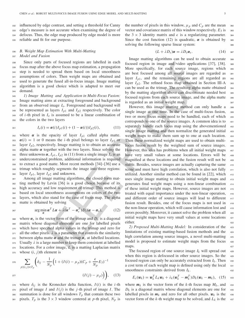
The weight maps using another matting based method IM561

in [22] and the proposed method are shown in Fig. 6b and 6d,562

respectively. To further demonstrate the effect of multi-563

matting, we replaced the multi-matting part with single image564

matting and normalization in each iteration of the proposed565

Fig. 6. (a) Source image. (b) Weight map using the IM method in [22].(c) Weight map of the proposed method using single image matting method.(d) Weight map of the proposed method using multi-matting method.

method, and the result is shown in Fig. 6c. Two regions are 566

selected to illustrate the benefit of multi-matting. The red box 567

is a boundary region of foreground and background. It is 568

obvious that the proposed method suppresses the excessive 569

spreading and gives a more exact location of the boundary. 570

The blue circle is a background region with a flat region on 571

the left and a boundary of the ‘clock’ on the right. It is hard 572

for single image matting to extract the flat region with good 573

accuracy and the errors cannot be eliminated in the iterative 574

refinement. The weight map values relate to the proportion 575

of the corresponding source image in the final fused image. 576

Since the background of the source image in Fig. 6a is heavily 577

blurred, the weight maps shown in Fig. 6b and 6c will produce 578

blur at the boundary of the ‘clock’ in background. In summary, 579

multi-matting generates exact location of the boundary and 580

iterative refinement makes the weight maps close to 0 or 1. 581

It should be noted that for color source images, we use 582

luminance values to estimate traditional focus measure and 583

edge model parameters as described in Section III-A. Then 584

RGB values are used in multi-matting model as described in 585

Section III-B because RGB values can provide more informa- 586

tion for image matting than luminance values. 587

IV. EXPERIMENT RESULTS AND DISCUSSIONS 588

A. Experimental Setup 589

Experiments were conducted on 36 sets of multi-focus 590

images, all of which are publicly available. 20 sets of them 591

come from a new multi-focus dataset called “Lytro” which is 592

publicly available online [41]. The other 16 sets are collected 593

IEEE P

roof


Fig. 7. A portion of the image sets used in our experiments.

online, which consist of one set of medical multi-focus images594

“bug” used in “Digital Photomontage” project [42], one set of595

Infrared multi-focus images “IR1g”, and another 14 sets which596

are widely used in multi-focus fusion research. The diversity597

of the image sets provides a good representation of various598

situations encountered in practice. A portion of the image sets599

are shown in Fig. 7.600

The proposed EMAM fusion method is compared601

with six multi-focus image fusion algorithms which are602

non-subsampled contourlet transform (NSCT) [8], guided603

filtering (GF) [11], image matting(IM) [22], sparse represen-604

tation (SR) [12], non-subsampled contourlet transform and605

sparse representation (NSCT-SR) [43], and dense scale invari-606

ant feature transform (DSIFT) [20]. Codes of all these methods607

are obtained online or directly from the authors, and the608

default parameters provided by the authors are adopted to keep609

consistency with the results given in the original papers.610

B. Objective Image Fusion Quality Metrics611

To evaluate the performance of different fusion methods612

objectively, several fusion quality metrics are needed. Since613

ground truth results for the case of multi-focus image fusion614

are usually not available, non-referenced quality metrics are615

generally preferred. A good survey of these kind of metrics616

can be found in [44]. Four quality metrics are adopted in this617

paper, which are also widely used in many related papers.618

For these four metrics, larger value means better fusion result.619

Default parameters provided by respective papers are used and620

details of these quality metrics are introduced as follows.621

1) Normalized Mutual Information (QN M I ): QN M I is an622

information theory based metric which measures the amount623

of original information in source images that is maintained624

in the fused image. Hossny et al. [46] modified the unstable625

traditional mutual information metric [45] to a normalized626

mutual information metric which is defined as627

QN M I = 2

[M I (A, F)

H (A) + H (F)+ M I (B, F)

H (B) + H (F)

], (22)628

where H (A), H (B) and H (F) are the marginal entropy of629

source image A, B and fused image F respectively. M I (A, F)630

is the mutual information between image A and F , which is631

defined as M I (A, F) = H (A) + H (F) − H (A, F). H (A, F)632

is the joint entropy between image A and F . M I (B, F) can633

be obtained similarly.634

2) Gradient-Based Fusion Performance (QG): This gra- 635

dient based metric is proposed to evaluate how well the 636

sharpness information in source images is transferred to the 637

fused image [47]. 638

QG 639

=∑N1

x=1

∑N2y=1(ϕ

A(x, y)AF (x, y) + ϕB(x, y)B F (x, y))∑N1

x=1

∑N2y=1(ϕ

A(x, y) + ϕB(x, y)), 640

(23) 641

where N1 and N2 are the width and height of a source 642

image respectively. AF is the element-wise product of edge 643

strength AFg and orientation preservation value AF

o of 644

source image A. B F is similarly defined for source image B . 645

ϕ A and ϕB are weighting coefficients that reflect the impor- 646

tance of AF and B F respectively. 647

3) Yang’s Metric (QY ): The structural similarity 648

(SSI M) [48] is used to derive Yang’s metric, which 649

measures the amount of structural information in source 650

images A and B that is preserved in the fused image F [49]. 651

QY =

⎧⎪⎪⎪⎨⎪⎪⎪⎩

γT SSIM(A, F |T ) + (1 − γT )SSIM(B, F |T ),

if SSIM(A, B|T ) ≥ 0.75

max{SSIM(A, F |T ), SSIM(B, F |T )},if SSIM(A, B|T ) < 0.75

(24) 652

where SSIM(·|T ) is the structural similarity in a local win- 653

dow T and γT = v(A|T )/(v(A|T ) + v(B|T )) is the local 654

weight derived from the local variance v(A|T ) and v(B|T ) 655

within the window T . 656

4) Chen-Blum Metric (QC B): This metric proposed in 657

Chen and Blum’s work [50] computes how well the contrast 658

features are preserved in fused image. Filtering is implemented 659

to each source image and the fused image in the frequency 660

domain. Then masked contrast maps for these images are 661

calculated by the information preservation value map whose 662

detailed definition can be found in [50]. Metric value is then 663

obtained as follows. 664

QC B 665

=∑N1

x=1

∑N2y=1(�A(x, y)PAF (x, y) + �B(x, y)PB F (x, y))

N1 N2, 666

(25) 667

where N1 and N2 are the width and height of the image, 668

�A and �B are the saliency maps for the source image 669

A and B , respectively. PAF and PB F are the information 670

preservation value maps. These two maps are computed from 671

the masked contrast map. 672

C. Parameters Setting 673

When calculating the focus measure in (7), the selection 674

of a large block size r improves robustness to noise but 675

reduces spatial resolution [51]. A radius r = 7 has been found 676

experimentally to be a good tradeoff in this work. The two 677

threshold values in (8) and (9) are set to be F Mth = 0.02 678

and Rth = 1.2. The choice of these two parameters is based 679

on observations that a 7 × 7 block with visible texture should 680

IEEE P

roof


TABLE I

EVALUATION METRIC VALUES OF DIFFERENT FUSION METHODS. THE METRIC VALUES IS THE AVERAGE VALUES OF ALL 36 IMAGE SETS.THE NUMBERS IN PARENTHESES DENOTE THE NUMBER OF IMAGE SETS THAT THIS METHOD BEATS THE OTHER METHODS

Fig. 8. (a) QN M I values of different F Mth values. (b) QG values ofdifferent F Mth values. (c) QY values of different F Mth values. (d) QC Bvalues of different F Mth values.

have the focus measure larger than 0.02, and the ratio value681

in (9) should be at least 1.2 if this block in that image is682

identified better focused than the other images. Experiments683

were conducted to analyze the sensitivity of F Mth and Rth ,684

and results are plotted in Fig. 8 and Fig. 9 respectively. It can685

be seen that F Mth and Rth are stable in the nearby range of686

our choices 0.02 and 1.2, which are marked by the red spots.687

The threshold for edge width is set to be σth = 0.5, since it688

is shown in [26] that majority of sharp edges have σ smaller689

than 0.5. It is shown in Fig. 10 that the setting of σth is stable690

in the nearby range of 0.5. Following the settings of image691

matting in [36], we set the parameter λ in (16) to be a large692

value 10 to keep wk and mk consistent at labelled locations.693

Since the choice of parameters is based on general properties694

of focus measure and edge model, this universal setting is695

independent to image content and provides good fusion results696

for all sets of multi-focus images.697

D. Experimental Results and Discussion698

1) Objective Evaluation Results: Objective evaluation699

results of different methods are shown in Table I, all of which700

are the average metric values over the whole 36 sets of images.701

The numbers in parentheses denote the number of image sets702

that this method surpasses the other methods. It is shown that703

the proposed EMAM fusion method clearly outperforms the704

other six methods in most cases in terms of the four different705

evaluation metrics, except QN M I in some sets of test images.706

A brief explanation about this is provided here. QN M I is a707

good metric since it estimates the mutual information between708

Fig. 9. (a) QN M I values of different Rth values. (b) QG values of differentRth values. (c) QY values of different Rth values. (d) QC B values of differentRth values.

Fig. 10. (a) QN M I values of different σth values. (b) QG values of differentσth values. (c) QY values of different σth values. (d) QC B values of differentσth values.

source images and fused image. But it does not consider 709

whether the local structure of source images is well preserved. 710

It is also reported in [11] that a very high QN M I value doesn’t 711

always mean good performance. The QN M I value tends to 712

be larger when the pixel values of the final fused image are 713

closer to one of the source images regardless of whether it 714

is focused or not. A simple test using the ‘block’ image set 715

was conducted and the results are shown in Table II. The 716

QN M I value when using one of the source images directly as 717

fusion result is dramatically elevated. The DSIFT method uses 718

IEEE P

roof


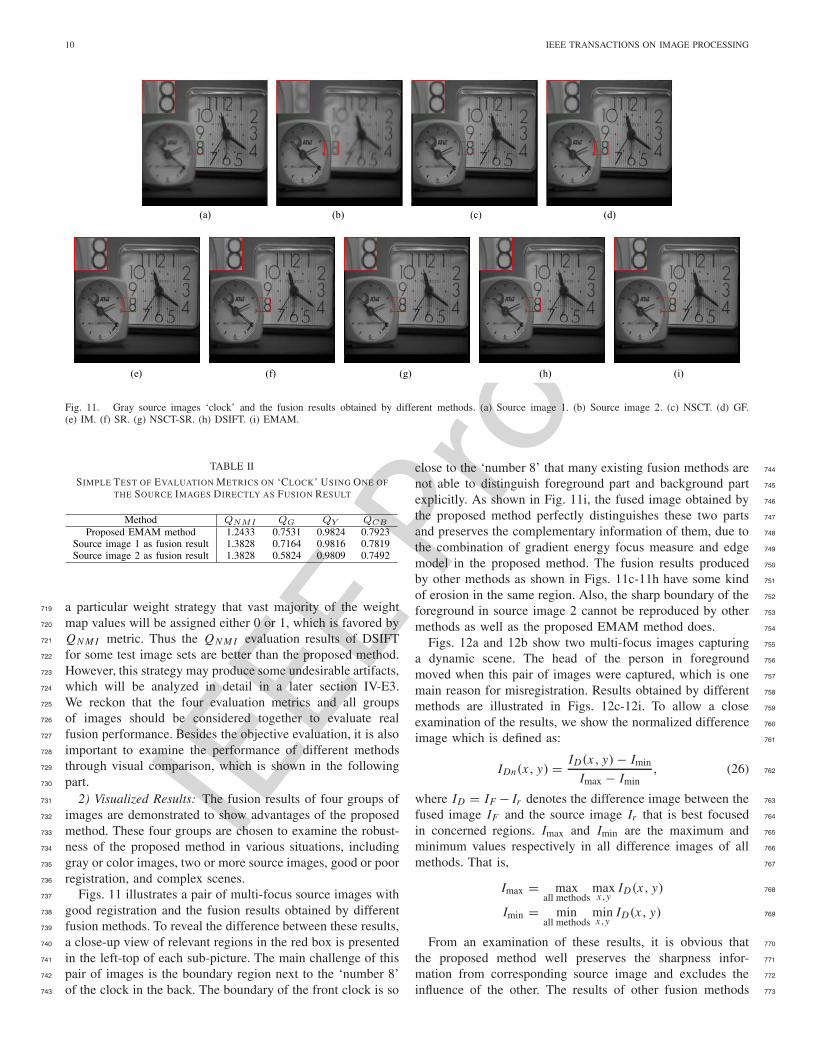
Fig. 11. Gray source images ‘clock’ and the fusion results obtained by different methods. (a) Source image 1. (b) Source image 2. (c) NSCT. (d) GF.(e) IM. (f) SR. (g) NSCT-SR. (h) DSIFT. (i) EMAM.

TABLE II

SIMPLE TEST OF EVALUATION METRICS ON ‘CLOCK’ USING ONE OF

THE SOURCE IMAGES DIRECTLY AS FUSION RESULT

a particular weight strategy that vast majority of the weight719

map values will be assigned either 0 or 1, which is favored by720

QN M I metric. Thus the QN M I evaluation results of DSIFT721

for some test image sets are better than the proposed method.722

However, this strategy may produce some undesirable artifacts,723

which will be analyzed in detail in a later section IV-E3.724

We reckon that the four evaluation metrics and all groups725

of images should be considered together to evaluate real726

fusion performance. Besides the objective evaluation, it is also727

important to examine the performance of different methods728

through visual comparison, which is shown in the following729

part.730

2) Visualized Results: The fusion results of four groups of731

images are demonstrated to show advantages of the proposed732

method. These four groups are chosen to examine the robust-733

ness of the proposed method in various situations, including734

gray or color images, two or more source images, good or poor735

registration, and complex scenes.736

Figs. 11 illustrates a pair of multi-focus source images with737

good registration and the fusion results obtained by different738

fusion methods. To reveal the difference between these results,739

a close-up view of relevant regions in the red box is presented740

in the left-top of each sub-picture. The main challenge of this741

pair of images is the boundary region next to the ‘number 8’742

of the clock in the back. The boundary of the front clock is so743

close to the ‘number 8’ that many existing fusion methods are 744

not able to distinguish foreground part and background part 745

explicitly. As shown in Fig. 11i, the fused image obtained by 746

the proposed method perfectly distinguishes these two parts 747

and preserves the complementary information of them, due to 748

the combination of gradient energy focus measure and edge 749

model in the proposed method. The fusion results produced 750

by other methods as shown in Figs. 11c-11h have some kind 751

of erosion in the same region. Also, the sharp boundary of the 752

foreground in source image 2 cannot be reproduced by other 753

methods as well as the proposed EMAM method does. 754

Figs. 12a and 12b show two multi-focus images capturing 755

a dynamic scene. The head of the person in foreground 756

moved when this pair of images were captured, which is one 757

main reason for misregistration. Results obtained by different 758

methods are illustrated in Figs. 12c-12i. To allow a close 759

examination of the results, we show the normalized difference 760

image which is defined as: 761

IDn(x, y) = ID(x, y) − Imin

Imax − Imin, (26) 762

where ID = IF − Ir denotes the difference image between the 763

fused image IF and the source image Ir that is best focused 764

in concerned regions. Imax and Imin are the maximum and 765

minimum values respectively in all difference images of all 766

methods. That is, 767

Imax = maxall methods

maxx,y

ID(x, y) 768

Imin = minall methods

minx,y

ID(x, y) 769

From an examination of these results, it is obvious that 770

the proposed method well preserves the sharpness infor- 771

mation from corresponding source image and excludes the 772

influence of the other. The results of other fusion methods 773

IEEE P

roof


Fig. 12. Gray source images and the fusion results obtained by different methods. (a) Source image 1. (b) Source image 2. (c) NSCT. (d) GF. (e) IM.(f) SR. (g) NSCT-SR. (h) DSIFT. (i) EMAM.

Fig. 13. Normalized difference images in the red block between the Source 2 and each of the fused images in Fig. 12. (a) NSCT. (b) GF. (c) IM. (d) SR.(e) NSCT-SR. (f) DSIFT. (g) EMAM.

contain artifacts in the misregistration region in the red box.774

Normalized difference images of this misregistration region775

are generated using source image 2 as a reference, and a close-776

up view of them is provided in Fig. 13. The good results of777

the proposed multi-matting method is due to the emphasis of778

spatial consistency, which is not fully considered in multi-779

scale decomposition based methods and sparse representation780

methods. The results of IM method are presented in Fig. 12e781

and Fig. 13c, which also have good performance in the misreg-782

istration region. However, the artifacts in the upper boundary783

of the foreground, as shown in the blue circle in Fig. 12e,784

reveal its limitation compared to the proposed method.785

Figs. 14a-14c demonstrate a set of color images with786

zooming in and out effect, which is another reason for misreg-787

istration. This phenomenon widely exists when changing the788

focus setting to capture images that focus in different objects.789

As shown in Fig. 14j, the proposed method outperforms790

the other fusion methods(see Figs. 14d-14i). The selected791

region in the red box is a good example, where the other792

methods are more likely to produce artifacts such as color793

distortion. Even the state-of-the-art method GF suffers from794

halo artifact in that region. Normalized grayscale difference795

images of this region are generated using source image 3 as a796

reference, and a close-up view of them is provided in Fig. 15.797

The proposed method avoids the halo artifact and generates798

better results than the other methods, except for the DSIFT799

method whose results in this region are comparable to ours.800

However, comparison of selected region in the blue circle, 801

as shown in Fig. 14i and Fig. 14j, demonstrates the good 802

performance of the proposed method. This is because the 803

proposed multi-matting model is performed in RGB space, 804

while the DSIFT method is performed in grayscale. 805

Figs. 16a-16b demonstrate a pair of color images captured 806

at complex scenes, where the foreground is a steel mesh and 807

the background can be seen through the holes. This situation 808

is most challenging for spatial-based methods, since the shape 809

of the foreground is not regular. Undesirable artifacts may 810

appear at some narrow foreground regions, where block-based 811

focus measures cannot perform very well. The selected regions 812

in the red box and blur circle shown in Fig. 16 are good 813

examples, in which the spatial-based methods IM and DSIFT 814

mislabel many pixels and have obvious artifacts. The two 815

source images are with perfect registration, so the multi-scale 816

decomposition based methods and sparse representation meth- 817

ods may not suffer from halo and ringing artifacts as described 818

in previous examples. However, the fusion results of them 819

still looks blurry, especially at the boundary of foreground 820

and background. The blurry artifacts are more obvious in the 821

normalized difference images as shown in Fig. 17, which use 822

source image 2 as a reference. It can be seen that method 823

NSCT, SR, NSCT-SR and GF still have a lot of background 824

residuals in the two selected regions. The proposed method’s 825

results as shown in Fig. 16i and 17g have few artifacts with a 826

much clearer boundary of foreground and background. 827

IEEE P

roof


Fig. 14. Color source images ‘book’ and the fusion results obtained by different methods. (a) Source image 1. (b) Source image 2. (c) Source image 3.(d) NSCT. (e) GF. (f) IM. (g) SR. (h) NSCT-SR. (i) DSIFT. (j) EMAM.

Fig. 15. Normalized difference images in the red block between the Source 3 and each of the fused images in Fig. 14. (a) NSCT. (b) GF. (c) IM. (d) SR.(e) NSCT-SR. (f) DSIFT. (g) EMAM.

E. Additional Analysis828

1) Combination of Edge Model: To investigate the effect829

of edge model, an experiment was performed without using830

edge model while other parts of the proposed method remain831

the same. The final weight map of the foreground using the832

complete proposed method is shown in Fig. 18b, and the final833

weight map without using edge model is shown in Fig. 18c.834

It can be seen that the result without using edge model tends835

to erode and dilate in the red box, which will lead to poor836

performance in this boundary region of the final fusion result. 837

Edge model compensates the shortage of the traditional focus 838

measure in this region, and provides a proper guidance for the 839

following multi-matting procedure. The evaluation results are 840

listed in Table III, which also shows the benefit of using edge 841

model. 842

2) Robustness to Noise: To examine the robustness to noise 843

of the proposed method, experiments were conducted. The 844

‘clock’ image pair is used as an example for explanation and 845

IEEE P

roof


Fig. 16. Color source images and the fusion results obtained by different methods. (a) Source image 1. (b) Source image 2. (c) NSCT. (d) GF. (e) IM.(f) SR. (g) NSCT-SR. (h) DSIFT. (i) EMAM.

Fig. 17. Normalized difference images between the Source 2 and each of the fused images in Fig. 16. (a) NSCT. (b) GF. (c) IM. (d) SR. (e) NSCT-SR.(f) DSIFT. (g) EMAM.

TABLE III

EVALUATION METRIC VALUES OF THE PROPOSED METHODWITH AND WITHOUT USING EDGE MODEL

similar results were obtained using other image sets. Differ-846

ent levels of Gaussian noise were added to the two source847

images and the i -th noise level corresponds to noise variance848

σ 2n = 0.0003i . 40 levels of noise were used and source images849

of level 10, 20 and 40 are demonstrated in Fig. 19.850

All the seven methods were used to fuse the source images 851

of each noise level. Since there is no groundtruth fusion 852

results, the 4 quality metrics mentioned in Section IV-B 853

are used for evaluation. The evaluation results are shown 854

in Fig. 20, where each sub-figure demonstrates the change 855

of one quality metric as noise level grows. The red solid 856

lines in these figures represent the proposed method, and the 857

performance in metric QG ,Qy and QC B are still better than 858

the other methods as noise level grows. The performance 859

in metric QN M I is not as good as DSIFT whose weight 860

strategy is favored by QN M I metric. QN M I value tends to 861

be large when pixel values of the final fused image are 862

IEEE P

roof


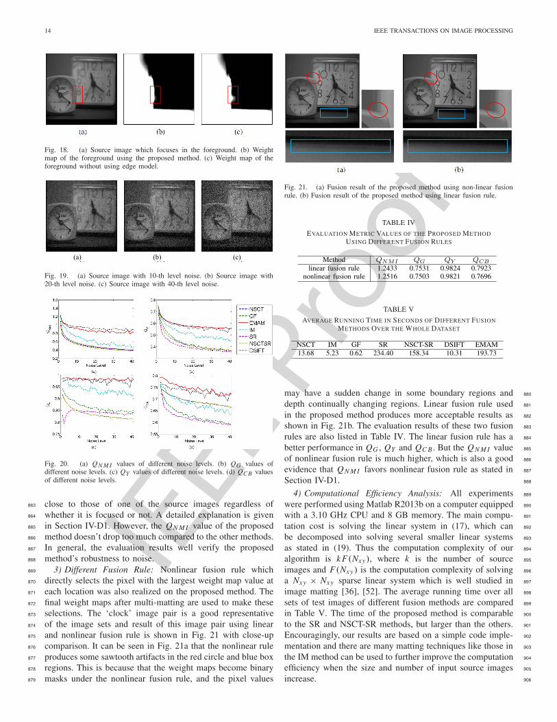
Fig. 18. (a) Source image which focuses in the foreground. (b) Weightmap of the foreground using the proposed method. (c) Weight map of theforeground without using edge model.

Fig. 19. (a) Source image with 10-th level noise. (b) Source image with20-th level noise. (c) Source image with 40-th level noise.

Fig. 20. (a) QN M I values of different noise levels. (b) QG values ofdifferent noise levels. (c) QY values of different noise levels. (d) QC B valuesof different noise levels.

close to those of one of the source images regardless of863

whether it is focused or not. A detailed explanation is given864

in Section IV-D1. However, the QN M I value of the proposed865

method doesn’t drop too much compared to the other methods.866

In general, the evaluation results well verify the proposed867

method’s robustness to noise.868

3) Different Fusion Rule: Nonlinear fusion rule which869

directly selects the pixel with the largest weight map value at870

each location was also realized on the proposed method. The871

final weight maps after multi-matting are used to make these872

selections. The ‘clock’ image pair is a good representative873

of the image sets and result of this image pair using linear874

and nonlinear fusion rule is shown in Fig. 21 with close-up875

comparison. It can be seen in Fig. 21a that the nonlinear rule876

produces some sawtooth artifacts in the red circle and blue box877

regions. This is because that the weight maps become binary878

masks under the nonlinear fusion rule, and the pixel values879

Fig. 21. (a) Fusion result of the proposed method using non-linear fusionrule. (b) Fusion result of the proposed method using linear fusion rule.

TABLE IV

EVALUATION METRIC VALUES OF THE PROPOSED METHOD

USING DIFFERENT FUSION RULES

TABLE V

AVERAGE RUNNING TIME IN SECONDS OF DIFFERENT FUSION

METHODS OVER THE WHOLE DATASET

may have a sudden change in some boundary regions and 880

depth continually changing regions. Linear fusion rule used 881

in the proposed method produces more acceptable results as 882

shown in Fig. 21b. The evaluation results of these two fusion 883

rules are also listed in Table IV. The linear fusion rule has a 884

better performance in QG , QY and QC B . But the QN M I value 885

of nonlinear fusion rule is much higher, which is also a good 886

evidence that QN M I favors nonlinear fusion rule as stated in 887

Section IV-D1. 888

4) Computational Efficiency Analysis: All experiments 889

were performed using Matlab R2013b on a computer equipped 890

with a 3.10 GHz CPU and 8 GB memory. The main compu- 891

tation cost is solving the linear system in (17), which can 892

be decomposed into solving several smaller linear systems 893

as stated in (19). Thus the computation complexity of our 894

algorithm is k F(Nxy), where k is the number of source 895

images and F(Nxy) is the computation complexity of solving 896

a Nxy × Nxy sparse linear system which is well studied in 897

image matting [36], [52]. The average running time over all 898

sets of test images of different fusion methods are compared 899

in Table V. The time of the proposed method is comparable 900

to the SR and NSCT-SR methods, but larger than the others. 901

Encouragingly, our results are based on a simple code imple- 902

mentation and there are many matting techniques like those in 903

the IM method can be used to further improve the computation 904

efficiency when the size and number of input source images 905

increase. 906

IEEE P

roof


V. CONCLUSIONS907

We have proposed an effective EMAM fusion method908

that outperforms current state-of-the-art fusion methods under909

various situations. The good performance is due to edge910

model and the multi-matting model. The combination of edge911

model and gradient energy focus measure well preserves912

the sharpness information in source images and defines the913

boundary of foreground and background accurately. The multi-914

matting model explicitly generates focus maps and weight915

maps efficiently in a single optimization problem, and has916

good performance in boundary and flat regions. These novel917

algorithms also make the proposed method robust to noise and918

misregistration in source images.919

APPENDIX920

DETAILS OF THE MATRIX COMPUTATION921

OF MULTI-MATTING922

Here we define923

w = [wT1 ,wT

2 , · · · ,wTN ]T ,924

S = [E, E, · · · , E]1×N ,925

where E is the identity matrix whose height and width are926

both equal to the number of pixels in one image,927

L = Diag(L1, L2, · · · , L N ),928

D = Diag(D1, D2, · · · , DN ),929

m = [mT1 , mT

2 , · · · , mTN ]T .930

So the linear system in (17) can be expressed as:931

[L + λD ST

S 0

][w

θ

]=

[λDm

e

],932

Here we use the properties of block matrix inversion to solve933

this linear system. First we calculate the Schur complement934

of the coefficient matrix.935

Sch = −S(L + λD)−1 ST936

Then we will have937

θ = −S−1ch S(L + λD)−1λDm + S−1

ch e938

w = (L + λD)−1(λDm − ST θ)939

Since L + λD is a diagonal block matrix, so the inverse of it940

(L +λD)−1 can be easily expressed using the inverse of each941

diagonal block.942

Diag((L1 + λD1)−1, (L2 + λD2)

−1, · · · , (L N + λDN )−1)943

Thus the Schur complement is944

Sch = −N∑

k=1

(Lk + λDk)−1.945

w can be calculated based on these properties: 946

w = (L + λD)−1λDm − (L + λD)−1 ST θ 947

=

⎡⎢⎢⎢⎣

(L1 + λD1)−1λD1m1

(L2 + λD2)−1λD2m2

...(L N + λDN )−1λDN mN

⎤⎥⎥⎥⎦ +

⎡⎢⎢⎢⎣

(L1 + λD1)−1S−1

ch e(L2 + λD2)

−1S−1ch e

...

(L N + λDN )−1S−1ch e

⎤⎥⎥⎥⎦ 948

+

⎡⎢⎢⎢⎣

(L1 + λD1)−1

(L2 + λD2)−1

...(L N + λDN )−1

⎤⎥⎥⎥⎦ S−1

ch

N∑

k=1

((Lk + λDk)−1λDk mk) 949

Thus each component of w can be obtained by 950

wk = (Lk + λDk)−1λDk mk 951

+ (Lk + λDk)−1S−1

ch

N∑

k=1

((Lk + λDk)−1λDk mk ) 952

− (Lk + λDk)−1S−1

ch e 953

= w0k + (Lk + λDk)−1S−1

ch (w0A − e). 954

ACKNOWLEDGMENT 955

The authors wish to thank Professor Zheng Liu for pro- 956

viding their code implementing objective quality metrics, 957

Professor Yu Liu for providing their MST-SR image fusion 958

toolbox and image dataset, Professor Peter Kovesi for provid- 959

ing their Computer Vision and Image Processing toolbox. 960

REFERENCES 961

[1] S. Li, X. Kang, L. Fang, J. Hu, and H. Yin, “Pixel-level image fusion: 962

A survey of the state of the art,” Inf. Fusion, vol. 33, pp. 100–112, 963

Jan. 2017. 964

[2] S. Li, B. Yang, and J. Hu, “Performance comparison of different multi- 965

resolution transforms for image fusion,” Inf. Fusion, vol. 12, pp. 74–84, 966

Apr. 2011. 967

[3] V. N. Gangapure, S. Banerjee, and A. S. Chowdhury, “Steerable local 968

frequency based multispectral multifocus image fusion,” Inf. Fusion, 969

vol. 23, pp. 99–115, May 2015. 970

[4] Y. P. Liu, J. Jin, Q. Wang, Y. Shen, and X. Dong, “Region level based 971

multi-focus image fusion using quaternion wavelet and normalized cut,” 972

Signal Process., vol. 97, pp. 9–30, Apr. 2014. 973

[5] J. J. Lewis, R. J. O’Callaghan, S. G. Nikolov, D. R. Bull, and 974

N. Canagarajah, “Pixel- and region-based image fusion with complex 975

wavelets,” Inf. Fusion, vol. 8, no. 2, pp. 119–130, 2007. 976

[6] L. Guo, M. Dai, and M. Zhu, “Multifocus color image fusion 977

based on quaternion curvelet transform,” Opt. Exp., vol. 20, no. 17, 978

pp. 18846–18860, 2012. 979

[7] Q.-G. Miao, C. Shi, P.-F. Xu, M. Yang, and Y.-B. Shi, “A novel 980

algorithm of image fusion using shearlets,” Opt. Commun., vol. 284, 981

no. 6, pp. 1540–1547, 2011. 982

[8] Q. Zhang and B.-L. Guo, “Multifocus image fusion using the non- 983

subsampled contourlet transform,” Signal Process., vol. 89, no. 7, 984

pp. 1334–1346, 2009. 985

[9] Y. Chai, H. Li, and X. Zhang, “Multifocus image fusion based on 986

features contrast of multiscale products in nonsubsampled contourlet 987

transform domain,” Optik-Int. J. Light Electron Opt., vol. 123, no. 7, 988

pp. 569–581, 2012. 989

[10] H. Zhao, Z. Shang, Y. Y. Tang, and B. Fang, “Multi-focus image 990

fusion based on the neighbor distance,” Pattern Recognit., vol. 46, 991

pp. 1002–1011, Mar. 2013. 992

[11] S. Li, X. Kang, and J. Hu, “Image fusion with guided filtering,” IEEE 993

Trans. Image Process., vol. 22, no. 7, pp. 2864–2875, Jul. 2013. 994

[12] B. Yang and S. Li, “Multifocus image fusion and restoration with sparse 995

representation,” IEEE Trans. Instrum. Meas., vol. 59, no. 4, pp. 884–892, 996

Apr. 2010. 997

IEEE P

roof


[13] Y. Liu and Z. Wang, “Simultaneous image fusion and denoising with998

adaptive sparse representation,” IET Image Process., vol. 9, no. 5,999

pp. 347–357, 2015.1000

[14] M. Nejati, S. Samavi, and S. Shirani, “Multi-focus image fusion using1001

dictionary-based sparse representation,” Inf. Fusion, vol. 25, pp. 72–84,1002

Sep. 2015.1003

[15] Q. Zhang and M. D. Levine, “Robust multi-focus image fusion using1004

multi-task sparse representation and spatial context,” IEEE Trans. Image1005

Process., vol. 25, no. 5, pp. 2045–2058, May 2016.1006

[16] K. Kodama and A. Kubota, “Efficient reconstruction of all-in-focus1007

images through shifted pinholes from multi-focus images for dense light1008

field synthesis and rendering,” IEEE Trans. Image Process., vol. 22,1009

no. 11, pp. 4407–4421, Nov. 2013.1010

[17] S. Li and B. Yang, “Multifocus image fusion using region segmentation1011

and spatial frequency,” Image Vis. Comput., vol. 26, no. 7, pp. 971–979,1012

2008.1013

[18] H. Li, Y. Chai, H. Yin, and G. Liu, “Multifocus image fusion and1014

denoising scheme based on homogeneity similarity,” Opt. Commun.,1015

vol. 285, no. 2, pp. 91–100, 2012.1016

[19] Y. Zhang, L. Chen, Z. Zhao, J. Jia, and J. Liu, “Multi-focus image1017

fusion based on robust principal component analysis and pulse-coupled1018

neural network,” Optik-Int. J. Light Electron Opt., vol. 125, no. 17,1019

pp. 5002–5006, 2014.1020

[20] Y. Liu, S. Liu, and Z. Wang, “Multi-focus image fusion with dense1021

SIFT,” Inf. Fusion, vol. 23, pp. 139–155, May 2015.1022

[21] S. Pertuz, D. Puig, M. A. Garcia, and A. Fusiello, “Generation of1023

all-in-focus images by noise-robust selective fusion of limited depth-1024

of-field images,” IEEE Trans. Image Process., vol. 22, no. 3,1025

pp. 1242–1251, Mar. 2013.1026

[22] S. Li, X. Kang, J. Hu, and B. Yang, “Image matting for fusion of1027

multi-focus images in dynamic scenes,” Inf. Fusion, vol. 14, no. 2,1028

pp. 147–162, 2013.1029

[23] Y. Chen and W.-K. Cham, “Edge model based fusion of multi-1030

focus images using matting method,” in Proc. IEEE Int. Conf. Image1031

Process. (ICIP), Sep. 2015, pp. 1840–1844.1032

[24] H.-Y. Lin and C.-H. Chang, “Depth from motion and defocus blur,” Opt.1033

Eng., vol. 45, no. 12, p. 127201, 2006.1034

[25] P. Favaro and S. Soatto, “A geometric approach to shape from defocus,”1035

IEEE Trans. Pattern Anal. Mach. Intell., vol. 27, no. 3, pp. 406–417,1036

Mar. 2005.1037

[26] P. J. L. van Beek, “Edge-based image representation and coding,”1038

M.S. thesis, Dept. Electr. Eng., Inf. Theory Group, Delft Univ. Technol.,1039

Delft, The Netherlands, 1995.1040

[27] G. Fan and W.-K. Cham, “Model-based edge reconstruction for low1041

bit-rate wavelet-compressed images,” IEEE Trans. Circuits Syst. Video1042

Technol., vol. 10, no. 1, pp. 120–132, Feb. 2000.1043

[28] J. Canny, “A computational approach to edge detection,” IEEE Trans.1044

Pattern Anal. Mach. Intell., vol. PAMI-8, no. 6, pp. 679–698, Nov. 1986.1045

[29] J. Guan, W. Zhang, J. Gu, and H. Ren, “No-reference blur assessment1046

based on edge modeling,” J. Vis. Commun. Image Represent., vol. 29,1047

pp. 1–7, May 2015.1048

[30] H. Mir, P. Xu, and P. van Beek, “An extensive empirical evaluation1049

of focus measures for digital photography,” Proc. SPIE, vol. 9023,1050

p. 90230I, Mar. 2014.AQ:1 1051

[31] S. Pertuz, D. Puig, and M. A. Garcia, “Analysis of focus measure1052

operators for shape-from-focus,” Pattern Recognit., vol. 46, no. 5,1053

pp. 1415–1432, 2013.1054

[32] M. Subbarao and J. K. Tyan, “Selecting the optimal focus measure1055

for autofocusing and depth-from-focus,” IEEE Trans. Pattern Anal.1056

Mach. Intell., vol. 20, no. 8, pp. 864–870, Aug. 1998.1057

[33] P. D. Kovesi. MATLAB and Octave Functions for Computer Vision1058

and Image Processing. [Online]. Available: http://www.peterkovesi.com/1059

matlabfns/AQ:2 1060

[34] J. Wang and M. F. Cohen, Image and Video Matting: A Survey. Breda,1061

The Netherlands: Now Publishers Inc., 2008.1062

[35] J. Wang and M. F. Cohen, “Optimized color sampling for robust1063

matting,” in Proc. IEEE Conf. Comput. Vis. Pattern Recognit. (CVPR),1064

Jun. 2007, pp. 1–8.1065

[36] A. Levin, D. Lischinski, and Y. Weiss, “A closed-form solution to natural1066

image matting,” IEEE Trans. Pattern Anal. Mach. Intell., vol. 30, no. 2,1067

pp. 228–242, Feb. 2008.1068

[37] H. Li and K. N. Ngan, “Unsupervized video segmentation with low1069

depth of field,” IEEE Trans. Circuits Syst. Video Technol., vol. 17, no. 12,1070

pp. 1742–1751, Dec. 2007.1071

[38] Z. Liu, W. Li, L. Shen, Z. Han, and Z. Zhang, “Automatic segmentation 1072

of focused objects from images with low depth of field,” Pattern 1073

Recognit. Lett., vol. 31, no. 7, pp. 572–581, 2010. 1074

[39] A. Levin, A. Rav Acha, and D. Lischinski, “Spectral matting,” IEEE 1075

Trans. Pattern Anal. Mach. Intell., vol. 30, no. 10, pp. 1699–1712, 1076

Oct. 2008. 1077

[40] P.-S. Liao, T.-S. Chen, and P.-C. Chung, “A fast algorithm for multilevel 1078

thresholding,” J. Inf. Sci. Eng., vol. 17, no. 5, pp. 713–727, 2001. 1079

[41] [Online]. Available: http://mansournejati.ece.iut.ac.ir/content/lytro- 1080

multi-focus-dataset AQ:31081

[42] [Online]. Available: http://grail.cs.washington.edu/projects/ 1082

photomontage/ 1083

[43] Y. Liu, S. Liu, and Z. Wang, “A general framework for image fusion 1084

based on multi-scale transform and sparse representation,” Inf. Fusion, 1085

vol. 24, pp. 147–164, Jul. 2015. 1086

[44] Z. Liu, E. Blasch, Z. Xue, J. Zhao, R. Laganiere, and W. Wu, “Objective 1087

assessment of multiresolution image fusion algorithms for context 1088

enhancement in night vision: A comparative study,” IEEE Trans. Pattern 1089

Anal. Mach. Intell., vol. 34, no. 1, pp. 94–109, Jan. 2012. 1090

[45] G. Qu, D. Zhang, and P. Yan, “Information measure for performance of 1091

image fusion,” Electron. Lett., vol. 38, no. 7, pp. 313–315, 2002. 1092

[46] M. Hossny, S. Nahavandi, and D. Creighton, “Comments on ‘Informa- 1093

tion measure for performance of image fusion,”’ Electron. Lett., vol. 44, 1094

no. 18, pp. 1066–1067, 2008. 1095

[47] C. S. Xydeas and V. Petrovic, “Objective image fusion performance 1096

measure,” Electron. Lett., vol. 36, no. 4, pp. 308–309, 2000. 1097

[48] Z. Wang, A. C. Bovik, H. R. Sheikh, and E. P. Simoncelli, “Image 1098

quality assessment: From error visibility to structural similarity,” IEEE 1099

Trans. Image Process., vol. 13, no. 4, pp. 600–612, Apr. 2004. 1100

[49] C. Yang, J.-Q. Zhang, X.-R. Wang, and X. Liu, “A novel similarity based 1101

quality metric for image fusion,” Inf. Fusion, vol. 9, no. 2, pp. 156–160, 1102

2008. 1103

[50] Y. Chen and R. S. Blum, “A new automated quality assessment algorithm 1104

for image fusion,” Image Vis. Comput., vol. 27, no. 10, pp. 1421–1432, 1105

2009. 1106

[51] A. S. Malik and T.-S. Choi, “Consideration of illumination effects and 1107

optimization of window size for accurate calculation of depth map for 1108

3D shape recovery,” Pattern Recognit., vol. 40, no. 1, pp. 154–170, 2007. 1109

[52] L. Grady, T. Schiwietz, S. Aharon, and R. Westermann, “Random 1110

walks for interactive alpha-matting,” in Proc. VIIP, vol. 2005. 2005, 1111

pp. 423–429. 1112

Yibo Chen received the B.Eng. degree in electronic 1113

engineering from Tsinghua University in 2012. He is 1114

currently pursuing the Ph.D. degree with the Depart- 1115

ment of Electronic Engineering, The Chinese Uni- 1116

versity of Hong Kong. His research interests include 1117

image processing, computer vision and machine 1118

learning, and specifically for multi-focus fusion. 1119

Jingwei Guan received the B.S. degree in control 1120

science and engineering from Shandong University, 1121

Jinan, China, in 2013, and the Ph.D. degree in 1122

electronic engineering from The Chinese University 1123

of Hong Kong, Hong Kong, in 2017. Her current 1124

interests include computer vision and deep learning. 1125

Wai-Kuen Cham received the degree in electronics 1126

from The Chinese University of Hong Kong in 1979, 1127

the M.Sc. and Ph.D. degrees from the Loughborough 1128

University of Technology, U.K., in 1980 and 1983, 1129

respectively. From 1984 to 1985, he was a Senior 1130

Engineer with Datacraft Hong Kong Ltd. and a 1131

Lecturer with the Department of Electronic Engi- 1132

neering, The Polytechnic University of Hong Kong. 1133

Since 1985, he has been with the Department of 1134

Electronic Engineering, The Chinese University of 1135

Hong Kong. 1136

ieee transactions on image processing 1 …ybchen/tip2017watermark.pdf · ieee proof ieee...

Documents