IEEE TRANSACTIONS ON IMAGE PROCESSING 1

3D Discrete Shearlet Transform and VideoProcessing

Pooran Singh Negi and Demetrio Labate

Abstract—In this paper, we introduce a digital implementationof the 3D shearlet transform and illustrate its application toproblems of video denoising and enhancement. The shearletrepresentation is a multiscale pyramid of well-localized wave-forms defined at various locations and orientations, which wasintroduced to overcome the limitations of traditional multiscalesystems in dealing with multidimensional data. While the shearletapproach shares the general philosophy of curvelets and sur-facelets, it is based on a very different mathematical frameworkwhich is derived from the theory of affine systems and usesshearing matrices rather than rotations. This allows a naturaltransition from the continuous to the digital setting and amore flexible mathematical structure. The 3D digital shearlettransform algorithm presented in this paper consists in a cascadeof a multiscale decomposition and a directional filtering stage.The filters employed in this decomposition are implemented asfinite-length filters and this ensures that the transform is localand numerically efficient. To illustrate its performance, the 3DDiscrete Shearlet Transform is applied to problems of videodenoising and enhancement, and compared against other state-of-the-art multiscale techniques, including curvelets and surfacelets.

Index Terms—Affine systems, curvelets, denoising, shearlets,sparsity, video processing, wavelets.

I. INTRODUCTIONThe shearlet representation, originally introduced in [1], [2],

has emerged in recent years as one of the most effective frame-works for the analysis and processing of multidimensionaldata. This representation is part of a new class of multiscalemethods introduced during the last 10 years with the goalto overcome the limitations of wavelets and other traditionalmethods through a framework which combines the standardmultiscale decomposition and the ability to efficiently captureanisotropic features. Other notable such methods include thecurvelets [3] and the contourlets [4]. Indeed, both curveletsand shearlets have been shown to form Parseval frames ofL2(R2) which are (nearly) optimally sparse in the class ofcartoon-like images, a standard model for images with edges[3], [5]. Specifically, if fM is the M term approximationobtained by selecting the M largest coefficients in the shearletor curvelet expansion of a cartoon-like image f , then theapproximation error satisfies the asymptotic estimate

||f − fSM ||22 ≍M−2(logM)3, as M → ∞.

Copyright (c) 2010 IEEE. Personal use of this material is permitted.However, permission to use this material for any other purposes must beobtained from the IEEE by sending a request to pubs-permissions@ieee.org.

P. S. Negi is with the Department of Mathematics, University of Houston,Houston, TX 77204, USA (e-mail:psnegi@math.uh.edu).

D. Labate is with the Department of Mathematics, University of Houston,Houston, TX 77204, USA (e-mail:dlabate@math.uh.edu).

EDICS: TEC-RST, TEC-MRS

Up to the log-like factor, this is the optimal approximation rate,in the sense that no other orthonormal systems or even framescan achieve a rate better than M−2. By contrast, waveletapproximations can only achieve a rate M−1 for functions inthis class [3]. Concerning the topic of sparse approximations, itis important to recall that the relevance of this notion goes farbeyond the applications to compression. In fact, constructingsparse representations for data in a certain class entails theintimate understanding of their true nature and structure, sothat sparse representations also provide the most effective toolfor tasks such as feature extraction and pattern recognition [6],[7].

Even though shearlets and curvelets share the same phi-losophy of combining multiscale and directional analysis andhave similar sparsity properties, they rely on a rather differentmathematical structure. In particular, the directionality of theshearlet systems is controlled through the use of shearing ma-trices rather than rotations, which are employed by curvelets.This offers the advantage of preserving the discrete integerlattice and enables a natural transition from the continuous tothe discrete setting. The contourlets, on the other hand, are apurely discrete framework, with the emphasis in the numericalimplementation rather than the continuous construction. Thespecial properties of the shearlet approach have been success-fully exploited in several imaging application. For example, thecombination of multiscale and directional decomposition usingshearing transformations is used to design powerful algorithmsfor image denoising in [7], [8]; the directional selectivity of theshearlet representation is exploited to derive very competitivealgorithms for edge detection and analysis in [9]; the sparsityof the shearlet representation is used to derive a very effectivealgorithm for the regularized inversion of the Radon transformin [10]. We also recall that a recent construction of compactlysupported shearlets appears to be promising in PDE’s and otherapplications [11], [12].

While directional multiscale systems such as curvelets andshearlets have emerged several years ago, only very recentlythe analysis of sparse representations using these representa-tions has been extended beyond dimension 2. This extensionis of great interest since many applications from areas suchas medical diagnostic, video surveillance and seismic imagingrequire to process 3D data sets, and sparse 3D representationsare very useful for the design of improved algorithms for dataanalysis and processing.

Notice that the formal extension of the construction ofmultiscale directional systems from 2D to 3D is not themajor challenge. In fact, 3D versions of curvelets have beenintroduced in [13], with the focus being on their discrete

−40−20

020

40

−40−20

020

40

−40

−20

0

20

40

ξ1ξ2

ξ3

−40−20

020

40

−40−20

020

40

−40

−30

−20

−10

0

10

20

30

40

ξ1ξ2

ξ3

−40−20

020

40

−40−20

020

40

−40

−30

−20

−10

0

10

20

30

40

ξ1ξ2

ξ3

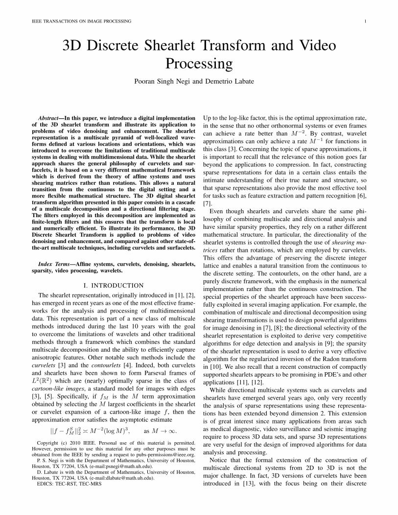
Fig. 1. From left to right, the figure illustrates the pyramidal regions P1, P2 and P3 in the frequency space R3.

implementations. Another discrete method is based on thesystem of surfacelets that were introduced as 3D extensionsof contourlets in [14]. However, the analysis of the sparsityproperties of curvelets or shearlets (or any other similarsystems) in the 3D setting does not follow directly from the2D argument. Only very recently [15], [16] it was shownby one of the authors in collaboration with K. Guo that 3Dshearlet representations exhibit essentially optimal approxima-tion properties for piecewise smooth functions of 3 variables.Namely, for 3D functions f which are smooth away fromdiscontinuities along C2 surfaces, it was shown that the Mterm approximation fSM obtained by selecting the N largestcoefficients in the 3D Parseval frame shearlet expansion of fsatisfies the asymptotic estimate

||f − fSM ||22 ≍M−1(logM)2, as M → ∞. (1)

Up to the logarithmic factor, this is the optimal decay rate andsignificantly outperforms wavelet approximations, which onlyyield a M−1/2 rate for functions in this class.

It is useful to recall that optimal approximation propertiesfor a large class of images can also be achieved using adaptivemethods by using, for example, the bandelets [17] or thegrouplets [18]. The shearlet approach, on the other hand,in non-adaptive. Remarkably, shearlets are able to achieveapproximation properties which are essentially as good as anadaptive approach when dealing with the class of cartoon-likeimages.

The objective of the paper is to present a numerical im-plementation of the 3D Discrete Shearlet Transform whichtakes advantage of the sparsity properties of the correspondingcontinuous representation. To illustrate the performance ofthis new numerical algorithm, we consider a number ofapplications to problems of video denoising and enhancement.As it will become apparent from the results presented below,not only our video processing algorithm based on the 3DDiscrete Shearlet Transform outperforms those based on thecorresponding 2D Discrete Shearlet Transform (when applied“slice by slice”), but it is also extremely competitive againstsimilar algorithms based on 3D curvelets and surfacelets.

II. SHEARLET REPRESENTATIONS

The shearlet approach provides a general method for theconstruction of function systems made up of functions rangingnot only at various scales and locations, but also according

to various orthogonal transformations controlled by shearingmatrices.

In dimension D = 3, a shearlet system is obtained byappropriately combining 3 systems of functions associatedwith the pyramidal regions

P1 =

{(ξ1, ξ2, ξ3) ∈ R3 : |ξ2

ξ1| ≤ 1, |ξ3

ξ1| ≤ 1

},

P2 =

{(ξ1, ξ2, ξ3) ∈ R3 : |ξ1

ξ2| < 1, |ξ3

ξ2| ≤ 1

},

P3 =

{(ξ1, ξ2, ξ3) ∈ R3 : |ξ1

ξ3| < 1, |ξ2

ξ3| < 1

},

in which the Fourier space R3 is partitioned (see Fig. 1).To define such systems, let ϕ be a C∞ univariate function

such that 0 ≤ ϕ ≤ 1, ϕ = 1 on [− 116 ,

116 ] and ϕ = 0 outside the

interval [−18 ,

18 ]. That is, ϕ is the scaling function of a Meyer

wavelet, rescaled so that its frequency support is contained theinterval [− 1

8 ,18 ]. For ξ = (ξ1, ξ2, ξ3) ∈ R3, define

Φ(ξ) = Φ(ξ1, ξ2, ξ3) = ϕ(ξ1) ϕ(ξ2) ϕ(ξ3) (2)

and let W (ξ) =

√Φ2(2−2ξ)− Φ2(ξ). It follows that

Φ2(ξ) +∑j≥0

W 2(2−2jξ) = 1 for ξ ∈ R3. (3)

Notice that each function Wj = W (2−2j ·), j ≥ 0, issupported inside the Cartesian corona

[−22j−1, 22j−1]3 \ [−22j−4, 22j−4]3 ⊂ R3,

and the functions W 2j , j ≥ 0, produce a smooth tiling of R3.

Next, let V ∈ C∞(R) be such that supp V ⊂ [−1, 1] and

|V (u− 1)|2 + |V (u)|2 + |V (u+1)|2 = 1 for |u| ≤ 1. (4)

In addition, we that V (0) = 1 and that V (n)(0) = 0 for alln ≥ 1. It was shown in [5] that there are several examples offunctions satisfying these properties. It follows from equation(4) that, for any j ≥ 0,

2j∑m=−2j

|V (2j u−m)|2 = 1, for |u| ≤ 1. (5)

2

For d = 1, 2, 3, ℓ = (ℓ1, ℓ2) ∈ Z2, the 3D shearlet systemsassociated with the pyramidal regions Pd are defined as thecollections

{ψ(d)j,ℓ,k : j ≥ 0,−2j ≤ ℓ1, ℓ2 ≤ 2j , k ∈ Z3}, (6)

where

ψ(d)j,ℓ,k(ξ) = | detA(d)|−

j2 W (2−2jξ)F(d)(ξA

−j(d)B

[−ℓ](d)

) e2πiξA

−j(d)

B[−ℓ](d)

k,

(7)F(1)(ξ1, ξ2, ξ3) = V ( ξ2ξ1 )V ( ξ3ξ1 ), F(2)(ξ1, ξ2, ξ3) =

V ( ξ1ξ2 )V ( ξ3ξ2 ), F(3)(ξ1, ξ2, ξ3) = V ( ξ1ξ3 )V ( ξ2ξ3 ), the anisotropicdilation matrices A(d) are given by

A(1) =

4 0 00 2 00 0 2

, A(2) =

2 0 00 4 00 0 2

, A(3) =

2 0 00 2 00 0 4

,and the shear matrices are defined by

B[ℓ](1)

=

1 ℓ1 ℓ20 1 00 0 1

, B[ℓ](2)

=

1 0 0ℓ1 1 ℓ20 0 1

, B[ℓ](3)

=

1 0 00 1 0ℓ1 ℓ2 1

.Due to the assumptions on W and v, the elements of the

system of shearlets (6) are well localized and bandlimited. Inparticular, the shearlets ψ(1)

j,ℓ,k(ξ) can be written more explicitlyas

ψ(1)j,ℓ,k(ξ) = 2−2j W (2−2jξ)V (2j ξ2

ξ1−ℓ1)V (2j ξ3

ξ1−ℓ2) e

2πiξA−j(1)

B[−ℓ](1)

k,

(8)showing that their supports are contained inside the trape-

zoidal regions

{(ξ1, ξ2, ξ3) : ξ1 ∈ [−22j−1,−22j−4] ∪ [22j−4, 22j−1],

|ξ2ξ1

− ℓ12−j | ≤ 2−j , |ξ3

ξ1− ℓ22

−j | ≤ 2−j}.

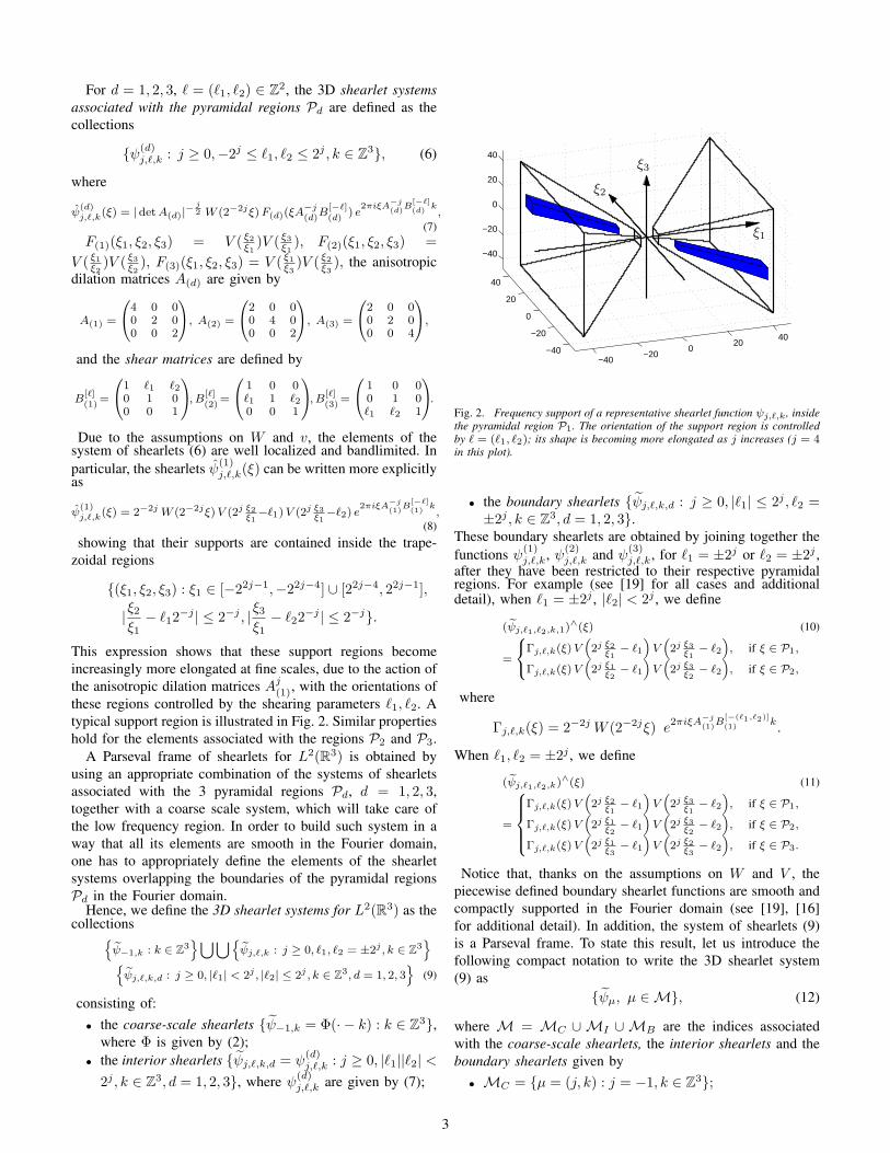
This expression shows that these support regions becomeincreasingly more elongated at fine scales, due to the action ofthe anisotropic dilation matrices Aj

(1), with the orientations ofthese regions controlled by the shearing parameters ℓ1, ℓ2. Atypical support region is illustrated in Fig. 2. Similar propertieshold for the elements associated with the regions P2 and P3.

A Parseval frame of shearlets for L2(R3) is obtained byusing an appropriate combination of the systems of shearletsassociated with the 3 pyramidal regions Pd, d = 1, 2, 3,together with a coarse scale system, which will take care ofthe low frequency region. In order to build such system in away that all its elements are smooth in the Fourier domain,one has to appropriately define the elements of the shearletsystems overlapping the boundaries of the pyramidal regionsPd in the Fourier domain.

Hence, we define the 3D shearlet systems for L2(R3) as thecollections{

ψ−1,k : k ∈ Z3}∪∪{

ψj,ℓ,k : j ≥ 0, ℓ1, ℓ2 = ±2j , k ∈ Z3}

{ψj,ℓ,k,d : j ≥ 0, |ℓ1| < 2j , |ℓ2| ≤ 2j , k ∈ Z3, d = 1, 2, 3

}(9)

consisting of:• the coarse-scale shearlets {ψ−1,k = Φ(· − k) : k ∈ Z3},

where Φ is given by (2);• the interior shearlets {ψj,ℓ,k,d = ψ

(d)j,ℓ,k : j ≥ 0, |ℓ1||ℓ2| <

2j , k ∈ Z3, d = 1, 2, 3}, where ψ(d)j,ℓ,k are given by (7);

−40−20

020

40

−40

−20

0

20

40

−40

−20

0

20

40

ξ1

ξ2

ξ3

Fig. 2. Frequency support of a representative shearlet function ψj,ℓ,k , insidethe pyramidal region P1. The orientation of the support region is controlledby ℓ = (ℓ1, ℓ2); its shape is becoming more elongated as j increases (j = 4in this plot).

• the boundary shearlets {ψj,ℓ,k,d : j ≥ 0, |ℓ1| ≤ 2j , ℓ2 =±2j , k ∈ Z3, d = 1, 2, 3}.

These boundary shearlets are obtained by joining together thefunctions ψ(1)

j,ℓ,k, ψ(2)j,ℓ,k and ψ(3)

j,ℓ,k, for ℓ1 = ±2j or ℓ2 = ±2j ,after they have been restricted to their respective pyramidalregions. For example (see [19] for all cases and additionaldetail), when ℓ1 = ±2j , |ℓ2| < 2j , we define

(ψj,ℓ1,ℓ2,k,1)∧(ξ) (10)

=

Γj,ℓ,k(ξ)V(2j ξ2

ξ1− ℓ1

)V(2j ξ3

ξ1− ℓ2

), if ξ ∈ P1,

Γj,ℓ,k(ξ)V(2j ξ1

ξ2− ℓ1

)V(2j ξ3

ξ2− ℓ2

), if ξ ∈ P2,

where

Γj,ℓ,k(ξ) = 2−2j W (2−2jξ) e2πiξA−j

(1)B

[−(ℓ1,ℓ2)]

(1)k.

When ℓ1, ℓ2 = ±2j , we define

(ψj,ℓ1,ℓ2,k)∧(ξ) (11)

=

Γj,ℓ,k(ξ)V

(2j ξ2

ξ1− ℓ1

)V(2j ξ3

ξ1− ℓ2

), if ξ ∈ P1,

Γj,ℓ,k(ξ)V(2j ξ1

ξ2− ℓ1

)V(2j ξ3

ξ2− ℓ2

), if ξ ∈ P2,

Γj,ℓ,k(ξ)V(2j ξ1

ξ3− ℓ1

)V(2j ξ2

ξ3− ℓ2

), if ξ ∈ P3.

Notice that, thanks on the assumptions on W and V , thepiecewise defined boundary shearlet functions are smooth andcompactly supported in the Fourier domain (see [19], [16]for additional detail). In addition, the system of shearlets (9)is a Parseval frame. To state this result, let us introduce thefollowing compact notation to write the 3D shearlet system(9) as

{ψµ, µ ∈ M}, (12)

where M = MC ∪ MI ∪ MB are the indices associatedwith the coarse-scale shearlets, the interior shearlets and theboundary shearlets given by

• MC = {µ = (j, k) : j = −1, k ∈ Z3};

3

• MI = {µ = (j, ℓ1, ℓ2, k, d) : j ≥ 0, |ℓ1|, |ℓ2| < 2j , k ∈Z3, d = 1, 2, 3};

• MB = {µ = (j, ℓ1, ℓ2, k, d) : j ≥ 0, |ℓ1| ≤ 2j , ℓ2 ±2j , k ∈ Z3, d = 1, 2, 3}.

Hence we have the following result whose proof is foundin [19]:

Theorem 1: The 3D system of shearlets (12) is a Parsevalframe of L2(R3). That is, for any f ∈ L2(R3),∑

µ∈M

|⟨f, ψµ⟩|2 = ∥f∥2.

The mapping from f ∈ L2(R3) into the elements ⟨f, ψµ⟩,µ ∈ M, is called the 3D shearlet transform.

As mentioned above, it is proved in [15], [16] that the3D Parseval frame of shearlets {ψµ, µ ∈ M} achieves theessentially optimal approximation rate (1) for functions of3 variables which are C2 regular away from discontinuitiesalong C2 surfaces.

III. 3D DISCRETE SHEARLET TRANSFORM (3D DSHT)

In this section, we present a digital implementation of the3D shearlet transform introduced above. Following essentiallythe same architecture as the algorithm of the 2D DiscreteShearlet Transform in [8], this new implementation can bedescribed as the cascade of a multiscale decomposition, basedon a version of the Laplacian pyramid filter, followed by astage of directional filtering. The main novelty of the 3Dapproach consists in the design of the directional filteringstage, which attempts to faithfully reproduce the frequencydecomposition provided by the corresponding mathematicaltransform by using a method based on the pseudo-sphericalFourier transform.

Let us start by expressing the elements of the shearletsystem in a form that is more convenient for deriving analgorithmic implementation of the shearlet transform. Forξ = (ξ1, ξ2, ξ3) in R3, j ≥ 0, and −2j ≤ ℓ1, ℓ2 ≤ 2j , wedefine the directional windowing functions

U(1)j,ℓ (ξ) =

V (2j ξ2ξ1

− ℓ1)V (2j ξ3ξ1

− ℓ2) if |ℓ1|, |ℓ2| < 2j ;

V (2j ξ2ξ1

− ℓ1)V (2j ξ3ξ1

− ℓ2)XP1 (ξ)

+V (2j ξ1ξ2

− ℓ1)V (2j ξ3ξ2

− ℓ2)XP2(ξ) if ℓ1 = ±2j , |ℓ2| < 2j ;

V (2j ξ2ξ1

− ℓ1)V (2j ξ3ξ1

− ℓ2)XP1 (ξ)

+V (2j ξ1ξ2

− ℓ1)V (2j ξ3ξ2

− ℓ2)XP2 (ξ)

+V (2j ξ1ξ3

− ℓ1)V (2j ξ2ξ3

− ℓ2)XP3 (ξ) if ℓ1, ℓ2 = ±2j .

Notice that only the elements U (1)j,ℓ with indices |ℓ1|, |ℓ2| <

2j are strictly contained inside the region P1; the elementswith indices ℓ1 = ±2j or ℓ2 = ±2j are supported across P1

and some other pyramidal region. However, it is convenient toassociate this family of functions with the index 1. We definethe functions U

(2)j,ℓ and U

(3)j,ℓ associated with the pyramidal

regions P2 and P3 in a similar way 1. Using this notation, wecan write each element of the 3D shearlet system as

ψ(d)j,ℓ,k = 2−2j W (2−2jξ)U

(d)j,ℓ (ξ) e

−2πiξA−j(d)

B[−ℓ]d k

.

1Notice however that they do not contain the boundary term for ℓ1, ℓ2 =±2j , which only needs to be included once.

It follows from the properties of the shearlet construction that

3∑d=1

∑j≥0

2j∑ℓ1=−2j

2j∑ℓ2=−2j

|W (2−2j(ξ)|2|U(d)j,ℓ (ξ)|

2 = 1, (13)

for |ξ1|, |ξ2|, |ξ3| ≥ 18 . The (fine scale) 3D shearlet transform

of f ∈ L(R3) can be expressed as the mapping from f intothe shearlet coefficients

⟨f, ψ(d)j,ℓ,k⟩ =

∫R3f(ξ)W (2−2jξ)U

(d)j,ℓ (ξ) e

2πiξA−j(d)

B[−ℓ](d)

kdξ, (14)

where j ≥ 0, ℓ = (ℓ1, ℓ2) with |ℓ1|, |ℓ2| ≤ 2j , k ∈ Z3 andd = 1, 2, 3.

This expression shows that the shearlet transform of f , forj, ℓ, k and d fixed, can be computed using the following steps:

1) In the frequency domain, compute the j-th subbanddecomposition of f as fj(ξ) = f(ξ)W (2−2jξ).

2) Next (still in the frequency domain), compute the(j, ℓ, d)-th directional subband decomposition of f asfj,ℓ,d(ξ) = fj(ξ)U

(d)j,ℓ (ξ).

3) Compute the inverse Fourier transform. This step canbe represented as a convolution of the j-th subbanddecomposition of f and the directional filter U (d)

j,ℓ , thatis, ⟨f, ψ(d)

j,ℓ,k⟩ = fj ∗ U (d)j,ℓ (A

−jd B−ℓ

d k).Hence, the shearlet transform of f can be described as acascade of subband decomposition and directional filteringstage.

A. 3D DShT Algorithm

The new numerical algorithm for computing the digitalvalues of the 3D shearlet transform, which is called 3D DShTalgorithm, will follow closely the 3 steps indicated above.

Before describing the numerical algorithm, let us recall thata digital 3D function f is an element of ℓ2(Z3

N ), where N ∈ N,that is, it consists of a finite array of values {f [n1, n2, n3] :n1, n2, n2 = 0, 1, 2, . . . , N − 1}. Here and in the following,we adopt the convention that a bracket [·, ·, ·] denotes an arrayof indices whereas the standard parenthesis (·, ·, ·) denotes afunction evaluation. Given a 3D digital function f ∈ ℓ2(Z3

N ),its Discrete Fourier Transform is given by:

f [k1, k2, k3] = N− 32

N−1∑n1,n2,n3=0

f [n1, n2, n3] e(−2πi(

n1N

k1+n2N

k2+n3N

k3))

for N2 ≤ k1, k2, k3 < N

2 . We shall interpret the numbersf [k1, k2, k3] as samples f [k1, k2, k3] = f(k1, k2, k3) from thetrigonometric polynomial

f(ξ1, ξ2, ξ3) = N− 32

N−1∑n1,n2,n3=0

f [n1, n2, n3] e(−2πi(

n1N

ξ1+n2N

ξ2+n3N

ξ3)).

We can now proceed with the description of the implemen-tation of the 3D DShT algorithm.

First, to calculate fj(ξ) in the digital domain, we performthe computation in the DFT domain as the product of theDFT of f and the DFT of the filters wj corresponding to thebandpass functions W (2−2j ·). This step can be implementedusing the Laplacian pyramid algorithm [20], which results inthe decomposition of the input signal f ∈ ℓ2(Z3

N ) into alow-pass and high-pass components. After extensive testing,

4

we found that a very satisfactory performance is achievedusing the modified version of the Laplacian pyramid algorithmdeveloped in [14]. For the first level of the decomposition, thisalgorithm downsamples the low-pass output by a non-integerfactor of 1.5 (upsampling by 2 followed by downsampling by3) along each dimension; the high-pass output is not down-sampled. In the subsequent decomposition stages, the low-passoutput is downsampled by 2 along each dimension and thehigh-pass output is not downsampled. Although the fractionalsampling factor in the first stage makes the algorithm slightlymore redundant than the traditional Laplacian pyramid, it wasfound that the added redundancy is very useful in reducingthe frequency domain aliasing (see [14] for more detail).

Next, one possible approach for computing the directionalcomponents fj,ℓ,d of f consists in resampling the j-th subbandcomponent of f into a pseudo-spherical grid and applyinga two-dimensional band-pass filter. Even though this is notthe approach we will use for our numerical experiments, themethod that we will use is conceptually derived from this one.

Recall that the pseudo-spherical grid is the 3D extensionof the 2D pseudo-polar grid and is parametrized by the planesgoing through the origin and their slopes. That is, the pseudo-spherical coordinates (u, v, w) ∈ R3 are given by

(u, v, w) =

(ξ1,

ξ2ξ1, ξ3ξ1 ) if (ξ1, ξ2, ξ3) ∈ DC1 ,

(ξ2,ξ1ξ2, ξ3ξ2 ) if (ξ1, ξ2, ξ3) ∈ DC2 ,

(ξ3,ξ1ξ3, ξ2ξ3 ) if (ξ1, ξ2, ξ3) ∈ DC3 .

Using this change of variables, it follows that fj,ℓ,d(ξ) can bewritten as

gj(u, v, w)U(d)(u, 2jv − ℓ1, 2

jw − ℓ2), (15)

where gj(u, v, w) is the function fj(ξ), after the change ofvariables, and U (d) = U

(d)0,0 . Notice that U (d) does not depend

on u. For example, when d = 1, the expression (15) can bewritten as

gj(u, v, w)V (2jv − ℓ1)V (2jw − ℓ2),

showing that the different directional components of fj areobtained by simply translating the window function V in thepseudo-spherical domain. In fact, this is a direct consequenceof using shearing matrices to control orientations and is itsmain advantage with respect to rotations. As a result, thediscrete samples gj [n1, n2, n3] = gj(n1, n2, n3) are the valuesof the DFT of fj [n1, n2, n3] on the pseudo-spherical grid andthey can be computed by direct reassignment or by adaptingthe Pseudo-polar DFT algorithm [21], [22] to the 3D setting.The 3D Pseudo-polar DFT evaluates the Fourier transform ofthe data on the Pseudo-polar grid and is formally defined as

P1(f)(k, l, j) := f(k,− 2l

Nk,−2

2j

Nk),

P2(f)(k, l, j) := f(− 2l

Nk, k,−2

2j

Nk),

P3(f)(k, l, j) := f(− 2l

Nk,−2

2j

Nk, k),

for k = −2N2 , · · · ,

2N2 and l, k = −N

2 , · · · ,N2 .

Let {u(d)j,ℓ1,ℓ2[n2, n3] : n2, n3 ∈ Z} be the sequence whose

DFT gives the discrete samples of the window functionsU (d)(2jv− ℓ1, 2

jw− ℓ2). For example, when d = 1, we havethat u(1)j,ℓ1,ℓ2

[k2, k3] = V (2jk2 − ℓ1)V (2jk3 − ℓ2). Then, forfixed k1 ∈ Z, we have

F2

(F−1

2 (gj) ∗ u(d)j,ℓ1,ℓ2

[n2, n3])[k1, k2, k3]

= gj [k1, k2, k3]u(d)j,ℓ1,ℓ2

[k2, k3] (16)

where F2 is the two dimensional DFT, defined as

F2(f)[k2, k3] =1

N

N−1∑n2,n3=0

f [n2, n3] e(−2πi(

n2N k2+

n3N k3)),

for −N2 ≤ k2, k3 <

N2 . Equation (16) gives the algorithmic

procedure for computing the discrete samples of the right handside of (15). That is, the 3D shearlet coefficients (14) canbe calculated from equation (16) by computing the inversepseudo-spherical DFT by directly re-assembling the Cartesiansampled values and applying the inverse 3-dimensional DFT.

In fact, the last observation suggests an alternative approachfor computing the directional components fj,ℓ,d of f . Thisapproach was found to perform better and it was used toproduce the numerical results below. The main idea consistsin mapping the filters from the pseudo-spherical domain backinto the Cartesian domain and then perform a convolutionwith band-passed data, similar to one of the methods used forthe 2D setting in [8]. Specifically if ϕP is the mapping fromCartesian domain into the pseudo-spherical domain then the3D shearlet coefficients in the Fourier domain can be expressedas

ϕ−1P

(gj [k1, k2, k3]u

(d)j,ℓ1,ℓ2

[k2, k3]).

Following the approach in [8], this can be expressed as

ϕ−1P (gj [k1, k2, k3]) ϕ

−1P

(δP [k1, k2, k3]u

(d)j,ℓ1,ℓ2

[k2, k3]),

where δP is the DFT of the (discrete) delta distributionin the pseudo-spherical grid. Thus the 3D discrete shearletcoefficients in the Fourier domain can be expressed as

fj [k1, k2, k3] h(d)j,ℓ1,ℓ2

[k1, k2, k3],

where

h(d)j,ℓ1,ℓ2

[k1, k2, k3] = ϕ−1P

(δP [k1, k2, k3]u

(d)j,ℓ1,ℓ2

[k2, k3]).

Notice that the new filters h(d)j,ℓ1,ℓ2

are not obtained by asimple change of variables, but by applying a resamplingwhich converts the pseudo-spherical grid to a Cartesian grid.This resampling is done using a linear map where possiblyseveral points from the polar grid are mapped to the samepoint on the rectangular grid. Although these filters are notcompactly supported, they can be implemented with a matrixrepresentation that is smaller than the size of the data f , henceallowing to implement the computation of the 3D DShT usinga convolution in space domain. One benefit of this approachis that one does not need to resample the DFT of the data intoa pseudo-spherical grid, as required using the first method.

Since the computational effort is essentially determinedby the FFT which is used to transform data and compute

5

convolutions, it follows that the 3D DShT algorithm runs inO(N3 log(N)) operations.

B. Implementation issues.

In principle, for the implementation of the 3D DShT algo-rithm one can choose any collection of filters U (d)

j,ℓ as long asthe tiling condition (13) is satisfied. The simplest solution isto choose functions U (d)

j,ℓ which are characteristic functions ofappropriate trapezoidal regions in the frequency domain, butthis type of filters are poorly localized in space domain. To befaithful to the continuous construction and also to ensure welllocalized filters in the space domain, our implementation usesfilters of Meyer type. A similar choice was also found effectivein [8] for the 2D setting. As mentioned above, by taking theinverse DFT, it is possible to implement these filters usingmatrix representations of size L3 with L ≪ N , where N3 isthe data size. In the numerical experiment considered below,we have chosen L = 24, which was found to be a very goodcompromise between localization and computation times. Fi-nally, for the number of directional bands, our algorithm allowsus to choose a different number of directional bands in eachpyramidal region. The theory prescribes to choose a numbern of directional bands which, in each pyramidal region, growslike 22j , hence giving n = 4, 16, 64, . . . directional bands, asthe scale is becoming finer. As will discuss below, we foundit convenient to slightly modify this canonical choice in thevideo denoising applications.

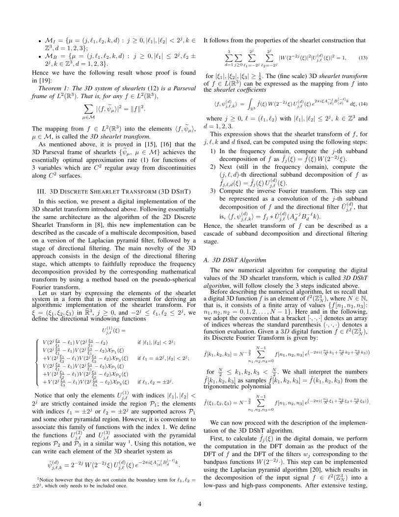
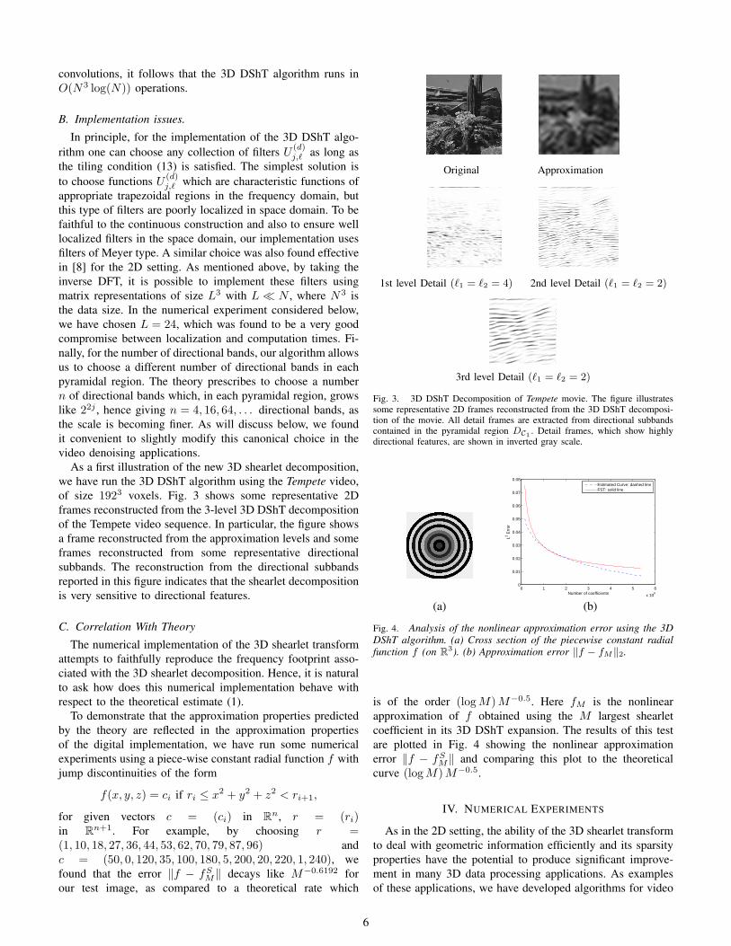
As a first illustration of the new 3D shearlet decomposition,we have run the 3D DShT algorithm using the Tempete video,of size 1923 voxels. Fig. 3 shows some representative 2Dframes reconstructed from the 3-level 3D DShT decompositionof the Tempete video sequence. In particular, the figure showsa frame reconstructed from the approximation levels and someframes reconstructed from some representative directionalsubbands. The reconstruction from the directional subbandsreported in this figure indicates that the shearlet decompositionis very sensitive to directional features.

C. Correlation With Theory

The numerical implementation of the 3D shearlet transformattempts to faithfully reproduce the frequency footprint asso-ciated with the 3D shearlet decomposition. Hence, it is naturalto ask how does this numerical implementation behave withrespect to the theoretical estimate (1).

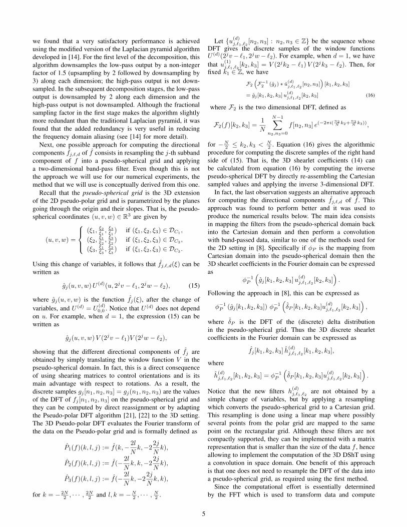
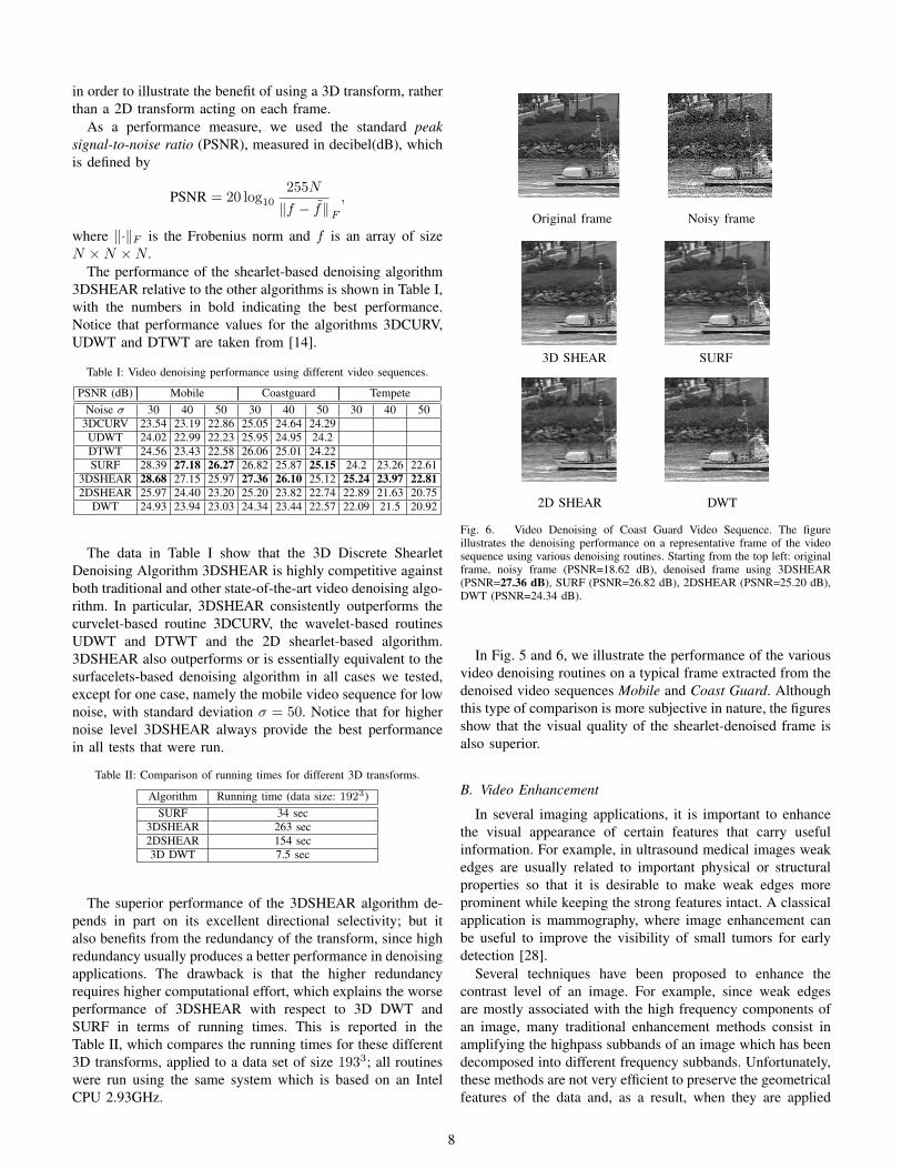
To demonstrate that the approximation properties predictedby the theory are reflected in the approximation propertiesof the digital implementation, we have run some numericalexperiments using a piece-wise constant radial function f withjump discontinuities of the form

f(x, y, z) = ci if ri ≤ x2 + y2 + z2 < ri+1,

for given vectors c = (ci) in Rn, r = (ri)in Rn+1. For example, by choosing r =(1, 10, 18, 27, 36, 44, 53, 62, 70, 79, 87, 96) andc = (50, 0, 120, 35, 100, 180, 5, 200, 20, 220, 1, 240), wefound that the error ∥f − fSM∥ decays like M−0.6192 forour test image, as compared to a theoretical rate which

Original Approximation

1st level Detail (ℓ1 = ℓ2 = 4) 2nd level Detail (ℓ1 = ℓ2 = 2)

3rd level Detail (ℓ1 = ℓ2 = 2)

Fig. 3. 3D DShT Decomposition of Tempete movie. The figure illustratessome representative 2D frames reconstructed from the 3D DShT decomposi-tion of the movie. All detail frames are extracted from directional subbandscontained in the pyramidal region DC1 . Detail frames, which show highlydirectional features, are shown in inverted gray scale.

0 1 2 3 4 5 6

x 108

0

0.01

0.02

0.03

0.04

0.05

0.06

0.07

0.08

Number of coefficients

L2 Err

or

Estimated Curve: dashed lineFST: solid line

(a) (b)

Fig. 4. Analysis of the nonlinear approximation error using the 3DDShT algorithm. (a) Cross section of the piecewise constant radialfunction f (on R3). (b) Approximation error ∥f − fM∥2.

is of the order (logM)M−0.5. Here fM is the nonlinearapproximation of f obtained using the M largest shearletcoefficient in its 3D DShT expansion. The results of this testare plotted in Fig. 4 showing the nonlinear approximationerror ∥f − fSM∥ and comparing this plot to the theoreticalcurve (logM)M−0.5.

IV. NUMERICAL EXPERIMENTS

As in the 2D setting, the ability of the 3D shearlet transformto deal with geometric information efficiently and its sparsityproperties have the potential to produce significant improve-ment in many 3D data processing applications. As examplesof these applications, we have developed algorithms for video

6

denoising and enhancement which are based on the new 3DDiscrete Shearlet Tranform presented above.

A. Video Denoising

The denoising of video is highly desirable for enhanced per-ceptibility, better compression and pattern recognition applica-tions. While noise can have different distributions like Poisson,Laplacian or Gaussian distribution, we only considered thesituation of zero-mean additive white Gaussian noise, whichoffers a good model for many practical situations. Hence, weassume that, for a given video f , we observe

y = f + n,

where n is Gaussian white noise with zero mean and standarddeviation σ.

It is well known that the ability to sparsely represent datais very useful in decorrelating the signal from the noise.This notion has been precisely formalized in the classicalwavelet shrinkage approach by Donoho and Johnstone [23],[24], which has lead to many successful denoising algorithms.In the following, we adapt this idea to design a simple videodenoising routine based on hard thresholding. That is, in ourapproach, we attempt to recover the video f from the observeddata y as follows.

1) We compute the 3D shearlet decomposition of y as y =∑µ⟨y, ψµ⟩ ψµ.

2) We set to zero the coefficients cµ(y) = ⟨y, ψµ⟩ such that|cµ(y)| < T , where T depends on the noise level.

3) We obtain an approximation f of f as f =∑µ c

∗µ(y) ψµ, where

c∗µ(y) =

{cµ(y) if |cµ(y)| ≥ T ;0 otherwise.

For the choice of the threshold parameter, we adopt the samecriterion which was found successful in the 2D setting, basedon the classical BayesShrink method [25]. This consists inchoosing

Tj,ℓ =σ2

σj,ℓ,

where σj,ℓ is the standard deviation of the shearlet coefficientsin the (j, ℓ)-th subband. Although hard thresholding is a rathercrude form of thresholding and more sophisticated methods areavailable, still this method is a good indication of the potentialof a transform in denoising applications. Also notice that hardthresholding performs better when dealing with data where it isimportant to preserve edges and sharp discontinuities (cf. [10],[26]).

For the 3D discrete shearlet decomposition, in all our testswe have applied a 3-level decomposition according to thealgorithm described above. For the number of directionalbands, we have chosen n = 16, 16, 64 (from the coarsestto the fines level) in each of the pyramidal region. Eventhough this does not exactly respect the rule canonical choice(n = 4, 16, 64) prescribed by the continuous model, we foundthat increasing the number of directional subbands at thecoarser level produces some improvement in the denoising

Original frame Noisy frame

3D SHEAR SURF

2D SHEAR DWT

Fig. 5. Video Denoising of Mobile Video Sequence. The figure comparesthe denoising performance of the denoising algorithm based on the 3D DShT,denoted as 3DSHEAR, on a representative frame of the video sequenceMobile against various video denoising routines. Starting from the top left:original frame, noisy frame (PSNR=18.62 dB, corresponding to σ = 30),denoised frame using 3DSHEAR (PSNR=28.68 dB), SURF (PSNR=28.39dB), 2DSHEAR (PSNR=25.97 dB) and DWT (PSNR=24.93 dB).

performance. Recall that, as indicated above, in our numericalimplementation, downsampling occurs only at the bandpasslevel, and there is no anisotropic down-sampling. Thus, thenumerical implementation of the 3D DShT which we foundmost effective in the denoising algorithm is highly redundant.Specifically, for data set of size N3, a 3-level 3D DShT decom-position produces 3∗

(64 ∗N3 + 16 ∗ ( 23N)3 + 16 ∗ ( 26N)3

)+

( 26N)3 ≈ 208 ∗ N3 coefficients. As we will see below(Table II), this requires a higher computational cost than lessredundant algorithms.

The 3D shearlet-based thresholding algorithm was testedon 3 video sequences, called mobile, coastguard and tempete,for various values of the standard deviation σ of the noise(values σ = 30, 40, 50 were considered). All these videosequences, which have been resized to 192×192×192, can beuploaded from the website http://www.cipr.rpi.edu.For a baseline comparison, we tested the performance ofthe shearlet-based denoising algorithm (denoted by 3DS-HEAR) against the following state-of-the-art algorithms: 3DCurvelets (denoted by 3DCURV, cf. [13]), Undecimated Dis-crete Wavelet Transform (denoted by UDWT, based on symletof length 16), Dual Tree Wavelet Transform (denoted byDTWT, cf. [27]) and Surfacelets (denoted by SURF, cf. [14]).We also compared against the 2D discrete shearlet transform(denoted by 2DSHEAR), which was applied frame by frame,

7

in order to illustrate the benefit of using a 3D transform, ratherthan a 2D transform acting on each frame.

As a performance measure, we used the standard peaksignal-to-noise ratio (PSNR), measured in decibel(dB), whichis defined by

PSNR = 20 log10255N

∥f − f∥F

,

where ∥·∥F is the Frobenius norm and f is an array of sizeN ×N ×N.

The performance of the shearlet-based denoising algorithm3DSHEAR relative to the other algorithms is shown in Table I,with the numbers in bold indicating the best performance.Notice that performance values for the algorithms 3DCURV,UDWT and DTWT are taken from [14].

Table I: Video denoising performance using different video sequences.

PSNR (dB) Mobile Coastguard TempeteNoise σ 30 40 50 30 40 50 30 40 50

3DCURV 23.54 23.19 22.86 25.05 24.64 24.29UDWT 24.02 22.99 22.23 25.95 24.95 24.2DTWT 24.56 23.43 22.58 26.06 25.01 24.22SURF 28.39 27.18 26.27 26.82 25.87 25.15 24.2 23.26 22.61

3DSHEAR 28.68 27.15 25.97 27.36 26.10 25.12 25.24 23.97 22.812DSHEAR 25.97 24.40 23.20 25.20 23.82 22.74 22.89 21.63 20.75

DWT 24.93 23.94 23.03 24.34 23.44 22.57 22.09 21.5 20.92

The data in Table I show that the 3D Discrete ShearletDenoising Algorithm 3DSHEAR is highly competitive againstboth traditional and other state-of-the-art video denoising algo-rithm. In particular, 3DSHEAR consistently outperforms thecurvelet-based routine 3DCURV, the wavelet-based routinesUDWT and DTWT and the 2D shearlet-based algorithm.3DSHEAR also outperforms or is essentially equivalent to thesurfacelets-based denoising algorithm in all cases we tested,except for one case, namely the mobile video sequence for lownoise, with standard deviation σ = 50. Notice that for highernoise level 3DSHEAR always provide the best performancein all tests that were run.

Table II: Comparison of running times for different 3D transforms.

Algorithm Running time (data size: 1923)SURF 34 sec

3DSHEAR 263 sec2DSHEAR 154 sec3D DWT 7.5 sec

The superior performance of the 3DSHEAR algorithm de-pends in part on its excellent directional selectivity; but italso benefits from the redundancy of the transform, since highredundancy usually produces a better performance in denoisingapplications. The drawback is that the higher redundancyrequires higher computational effort, which explains the worseperformance of 3DSHEAR with respect to 3D DWT andSURF in terms of running times. This is reported in theTable II, which compares the running times for these different3D transforms, applied to a data set of size 1933; all routineswere run using the same system which is based on an IntelCPU 2.93GHz.

Original frame Noisy frame

3D SHEAR SURF

2D SHEAR DWT

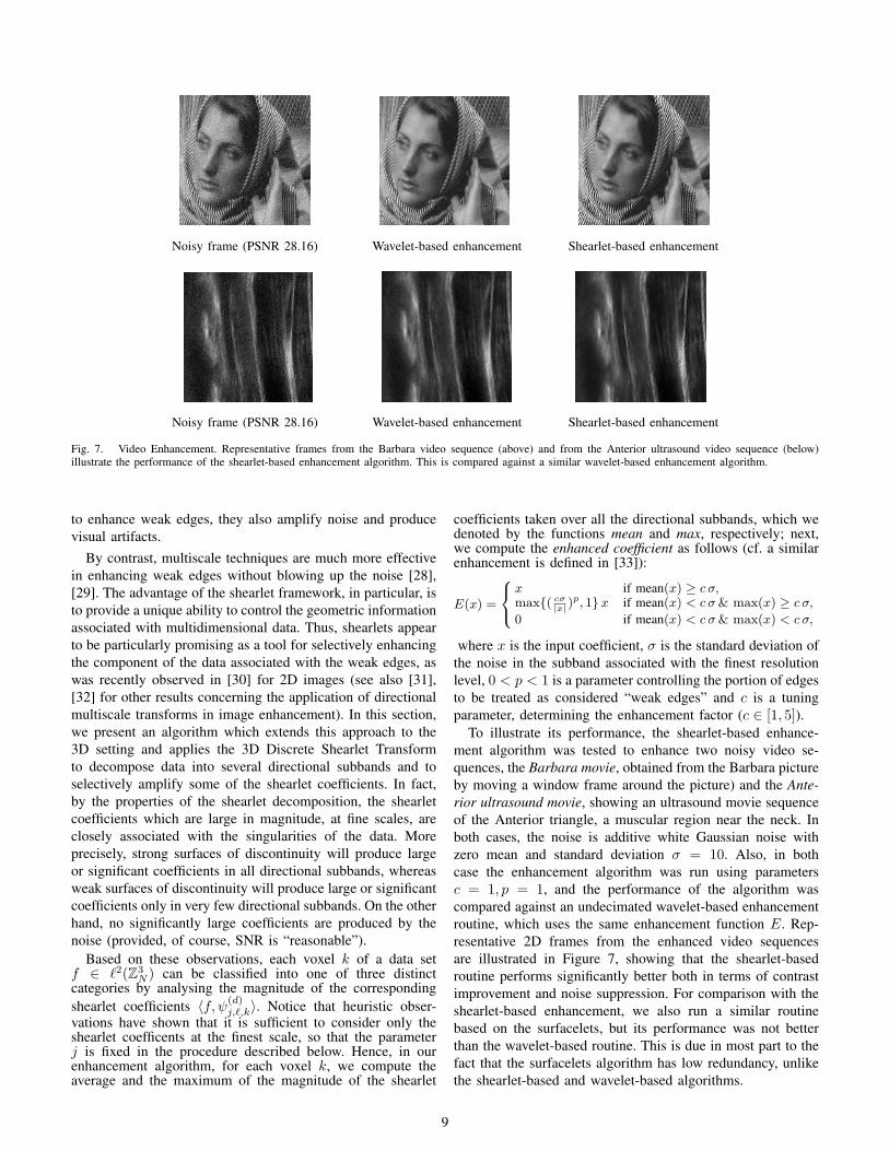
Fig. 6. Video Denoising of Coast Guard Video Sequence. The figureillustrates the denoising performance on a representative frame of the videosequence using various denoising routines. Starting from the top left: originalframe, noisy frame (PSNR=18.62 dB), denoised frame using 3DSHEAR(PSNR=27.36 dB), SURF (PSNR=26.82 dB), 2DSHEAR (PSNR=25.20 dB),DWT (PSNR=24.34 dB).

In Fig. 5 and 6, we illustrate the performance of the variousvideo denoising routines on a typical frame extracted from thedenoised video sequences Mobile and Coast Guard. Althoughthis type of comparison is more subjective in nature, the figuresshow that the visual quality of the shearlet-denoised frame isalso superior.

B. Video Enhancement

In several imaging applications, it is important to enhancethe visual appearance of certain features that carry usefulinformation. For example, in ultrasound medical images weakedges are usually related to important physical or structuralproperties so that it is desirable to make weak edges moreprominent while keeping the strong features intact. A classicalapplication is mammography, where image enhancement canbe useful to improve the visibility of small tumors for earlydetection [28].

Several techniques have been proposed to enhance thecontrast level of an image. For example, since weak edgesare mostly associated with the high frequency components ofan image, many traditional enhancement methods consist inamplifying the highpass subbands of an image which has beendecomposed into different frequency subbands. Unfortunately,these methods are not very efficient to preserve the geometricalfeatures of the data and, as a result, when they are applied

8

Noisy frame (PSNR 28.16) Wavelet-based enhancement Shearlet-based enhancement

Noisy frame (PSNR 28.16) Wavelet-based enhancement Shearlet-based enhancement

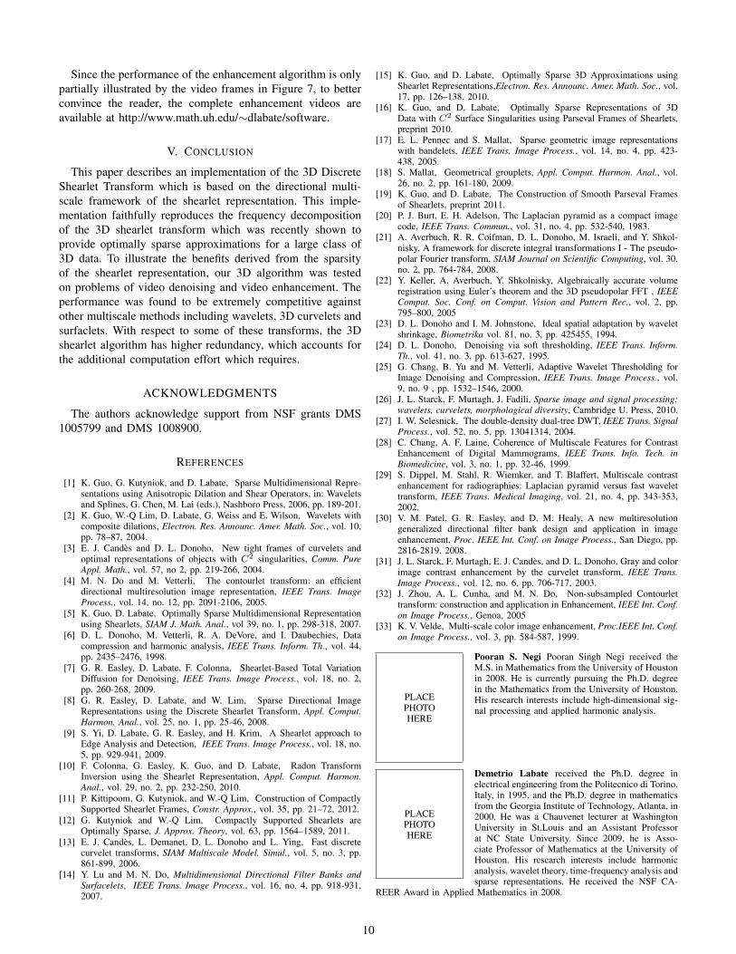
Fig. 7. Video Enhancement. Representative frames from the Barbara video sequence (above) and from the Anterior ultrasound video sequence (below)illustrate the performance of the shearlet-based enhancement algorithm. This is compared against a similar wavelet-based enhancement algorithm.

to enhance weak edges, they also amplify noise and producevisual artifacts.

By contrast, multiscale techniques are much more effectivein enhancing weak edges without blowing up the noise [28],[29]. The advantage of the shearlet framework, in particular, isto provide a unique ability to control the geometric informationassociated with multidimensional data. Thus, shearlets appearto be particularly promising as a tool for selectively enhancingthe component of the data associated with the weak edges, aswas recently observed in [30] for 2D images (see also [31],[32] for other results concerning the application of directionalmultiscale transforms in image enhancement). In this section,we present an algorithm which extends this approach to the3D setting and applies the 3D Discrete Shearlet Transformto decompose data into several directional subbands and toselectively amplify some of the shearlet coefficients. In fact,by the properties of the shearlet decomposition, the shearletcoefficients which are large in magnitude, at fine scales, areclosely associated with the singularities of the data. Moreprecisely, strong surfaces of discontinuity will produce largeor significant coefficients in all directional subbands, whereasweak surfaces of discontinuity will produce large or significantcoefficients only in very few directional subbands. On the otherhand, no significantly large coefficients are produced by thenoise (provided, of course, SNR is “reasonable”).

Based on these observations, each voxel k of a data setf ∈ ℓ2(Z3

N ) can be classified into one of three distinctcategories by analysing the magnitude of the correspondingshearlet coefficients ⟨f, ψ(d)

j,ℓ,k⟩. Notice that heuristic obser-vations have shown that it is sufficient to consider only theshearlet coefficents at the finest scale, so that the parameterj is fixed in the procedure described below. Hence, in ourenhancement algorithm, for each voxel k, we compute theaverage and the maximum of the magnitude of the shearlet

coefficients taken over all the directional subbands, which wedenoted by the functions mean and max, respectively; next,we compute the enhanced coefficient as follows (cf. a similarenhancement is defined in [33]):

E(x) =

x if mean(x) ≥ c σ,max{( cσ

|x| )p, 1}x if mean(x) < cσ& max(x) ≥ c σ,

0 if mean(x) < cσ& max(x) < cσ,

where x is the input coefficient, σ is the standard deviation ofthe noise in the subband associated with the finest resolutionlevel, 0 < p < 1 is a parameter controlling the portion of edgesto be treated as considered “weak edges” and c is a tuningparameter, determining the enhancement factor (c ∈ [1, 5]).

To illustrate its performance, the shearlet-based enhance-ment algorithm was tested to enhance two noisy video se-quences, the Barbara movie, obtained from the Barbara pictureby moving a window frame around the picture) and the Ante-rior ultrasound movie, showing an ultrasound movie sequenceof the Anterior triangle, a muscular region near the neck. Inboth cases, the noise is additive white Gaussian noise withzero mean and standard deviation σ = 10. Also, in bothcase the enhancement algorithm was run using parametersc = 1, p = 1, and the performance of the algorithm wascompared against an undecimated wavelet-based enhancementroutine, which uses the same enhancement function E. Rep-resentative 2D frames from the enhanced video sequencesare illustrated in Figure 7, showing that the shearlet-basedroutine performs significantly better both in terms of contrastimprovement and noise suppression. For comparison with theshearlet-based enhancement, we also run a similar routinebased on the surfacelets, but its performance was not betterthan the wavelet-based routine. This is due in most part to thefact that the surfacelets algorithm has low redundancy, unlikethe shearlet-based and wavelet-based algorithms.

9

Since the performance of the enhancement algorithm is onlypartially illustrated by the video frames in Figure 7, to betterconvince the reader, the complete enhancement videos areavailable at http://www.math.uh.edu/∼dlabate/software.

V. CONCLUSION

This paper describes an implementation of the 3D DiscreteShearlet Transform which is based on the directional multi-scale framework of the shearlet representation. This imple-mentation faithfully reproduces the frequency decompositionof the 3D shearlet transform which was recently shown toprovide optimally sparse approximations for a large class of3D data. To illustrate the benefits derived from the sparsityof the shearlet representation, our 3D algorithm was testedon problems of video denoising and video enhancement. Theperformance was found to be extremely competitive againstother multiscale methods including wavelets, 3D curvelets andsurfaclets. With respect to some of these transforms, the 3Dshearlet algorithm has higher redundancy, which accounts forthe additional computation effort which requires.

ACKNOWLEDGMENTS

The authors acknowledge support from NSF grants DMS1005799 and DMS 1008900.

REFERENCES

[1] K. Guo, G. Kutyniok, and D. Labate, Sparse Multidimensional Repre-sentations using Anisotropic Dilation and Shear Operators, in: Waveletsand Splines, G. Chen, M. Lai (eds.), Nashboro Press, 2006, pp. 189-201.

[2] K. Guo, W.-Q Lim, D. Labate, G. Weiss and E. Wilson, Wavelets withcomposite dilations, Electron. Res. Announc. Amer. Math. Soc., vol. 10,pp. 78–87, 2004.

[3] E. J. Candes and D. L. Donoho, New tight frames of curvelets andoptimal representations of objects with C2 singularities, Comm. PureAppl. Math., vol. 57, no 2, pp. 219-266, 2004.

[4] M. N. Do and M. Vetterli, The contourlet transform: an efficientdirectional multiresolution image representation, IEEE Trans. ImageProcess., vol. 14, no. 12, pp. 2091-2106, 2005.

[5] K. Guo, D. Labate, Optimally Sparse Multidimensional Representationusing Shearlets, SIAM J. Math. Anal., vol 39, no. 1, pp. 298-318, 2007.

[6] D. L. Donoho, M. Vetterli, R. A. DeVore, and I. Daubechies, Datacompression and harmonic analysis, IEEE Trans. Inform. Th., vol. 44,pp. 2435–2476, 1998.

[7] G. R. Easley, D. Labate, F. Colonna, Shearlet-Based Total VariationDiffusion for Denoising, IEEE Trans. Image Process., vol. 18, no. 2,pp. 260-268, 2009.

[8] G. R. Easley, D. Labate, and W. Lim, Sparse Directional ImageRepresentations using the Discrete Shearlet Transform, Appl. Comput.Harmon. Anal., vol. 25, no. 1, pp. 25-46, 2008.

[9] S. Yi, D. Labate, G. R. Easley, and H. Krim, A Shearlet approach toEdge Analysis and Detection, IEEE Trans. Image Process., vol. 18, no.5, pp. 929-941, 2009.

[10] F. Colonna, G. Easley, K. Guo, and D. Labate, Radon TransformInversion using the Shearlet Representation, Appl. Comput. Harmon.Anal., vol. 29, no. 2, pp. 232-250, 2010.

[11] P. Kittipoom, G. Kutyniok, and W.-Q Lim, Construction of CompactlySupported Shearlet Frames, Constr. Approx., vol. 35, pp. 21–72, 2012.

[12] G. Kutyniok and W.-Q Lim, Compactly Supported Shearlets areOptimally Sparse, J. Approx. Theory, vol. 63, pp. 1564–1589, 2011.

[13] E. J. Candes, L. Demanet, D. L. Donoho and L. Ying, Fast discretecurvelet transforms, SIAM Multiscale Model. Simul., vol. 5, no. 3, pp.861-899, 2006.

[14] Y. Lu and M. N. Do, Multidimensional Directional Filter Banks andSurfacelets, IEEE Trans. Image Process., vol. 16, no. 4, pp. 918-931,2007.

[15] K. Guo, and D. Labate, Optimally Sparse 3D Approximations usingShearlet Representations,Electron. Res. Announc. Amer. Math. Soc., vol.17, pp. 126–138, 2010.

[16] K. Guo, and D. Labate, Optimally Sparse Representations of 3DData with C2 Surface Singularities using Parseval Frames of Shearlets,preprint 2010.

[17] E. L. Pennec and S. Mallat, Sparse geometric image representationswith bandelets, IEEE Trans. Image Process., vol. 14, no. 4, pp. 423-438, 2005.

[18] S. Mallat, Geometrical grouplets, Appl. Comput. Harmon. Anal., vol.26, no. 2, pp. 161-180, 2009.

[19] K. Guo, and D. Labate, The Construction of Smooth Parseval Framesof Shearlets, preprint 2011.

[20] P. J. Burt, E. H. Adelson, The Laplacian pyramid as a compact imagecode, IEEE Trans. Commun., vol. 31, no. 4, pp. 532-540, 1983.

[21] A. Averbuch, R. R. Coifman, D. L. Donoho, M. Israeli, and Y. Shkol-nisky, A framework for discrete integral transformations I - The pseudo-polar Fourier transform, SIAM Journal on Scientific Computing, vol. 30,no. 2, pp. 764-784, 2008.

[22] Y. Keller, A. Averbuch, Y. Shkolnisky, Algebraically accurate volumeregistration using Euler’s theorem and the 3D pseudopolar FFT , IEEEComput. Soc. Conf. on Comput. Vision and Pattern Rec., vol. 2, pp.795–800, 2005

[23] D. L. Donoho and I. M. Johnstone, Ideal spatial adaptation by waveletshrinkage, Biometrika vol. 81, no. 3, pp. 425455, 1994.

[24] D. L. Donoho, Denoising via soft thresholding, IEEE Trans. Inform.Th., vol. 41, no. 3, pp. 613-627, 1995.

[25] G. Chang, B. Yu and M. Vetterli, Adaptive Wavelet Thresholding forImage Denoising and Compression, IEEE Trans. Image Process., vol.9, no. 9 , pp. 1532–1546, 2000.

[26] J. L. Starck, F. Murtagh, J. Fadili, Sparse image and signal processing:wavelets, curvelets, morphological diversity, Cambridge U. Press, 2010.

[27] I. W. Selesnick, The double-density dual-tree DWT, IEEE Trans. SignalProcess., vol. 52, no. 5, pp. 13041314, 2004.

[28] C. Chang, A. F. Laine, Coherence of Multiscale Features for ContrastEnhancement of Digital Mammograms, IEEE Trans. Info. Tech. inBiomedicine, vol. 3, no. 1, pp. 32-46, 1999.

[29] S. Dippel, M. Stahl, R. Wiemker, and T. Blaffert, Multiscale contrastenhancement for radiographies: Laplacian pyramid versus fast wavelettransform, IEEE Trans. Medical Imaging, vol. 21, no. 4, pp. 343-353,2002.

[30] V. M. Patel, G. R. Easley, and D. M. Healy, A new multiresolutiongeneralized directional filter bank design and application in imageenhancement, Proc. IEEE Int. Conf. on Image Process., San Diego, pp.2816-2819, 2008.

[31] J. L. Starck, F. Murtagh, E. J. Candes, and D. L. Donoho, Gray and colorimage contrast enhancement by the curvelet transform, IEEE Trans.Image Process., vol. 12, no. 6, pp. 706-717, 2003.

[32] J. Zhou, A. L. Cunha, and M. N. Do, Non-subsampled Contourlettransform: construction and application in Enhancement, IEEE Int. Conf.on Image Process., Genoa, 2005

[33] K. V. Velde, Multi-scale color image enhancement, Proc.IEEE Int. Conf.on Image Process., vol. 3, pp. 584-587, 1999.

PLACEPHOTOHERE

Pooran S. Negi Pooran Singh Negi received theM.S. in Mathematics from the University of Houstonin 2008. He is currently pursuing the Ph.D. degreein the Mathematics from the University of Houston.His research interests include high-dimensional sig-nal processing and applied harmonic analysis.

PLACEPHOTOHERE

Demetrio Labate received the Ph.D. degree inelectrical engineering from the Politecnico di Torino,Italy, in 1995, and the Ph.D. degree in mathematicsfrom the Georgia Institute of Technology, Atlanta, in2000. He was a Chauvenet lecturer at WashingtonUniversity in St.Louis and an Assistant Professorat NC State University. Since 2009, he is Asso-ciate Professor of Mathematics at the University ofHouston. His research interests include harmonicanalysis, wavelet theory, time-frequency analysis andsparse representations. He received the NSF CA-

REER Award in Applied Mathematics in 2008.

10