ieee transactions on geoscience and …dclausi/papers/published 2004/clausi and yue...random fields...

IEEE TRANSACTIONS ON GEOSCIENCE AND REMOTE SENSING, VOL. 42, NO. 1, JANUARY 2004 215

Comparing Cooccurrence Probabilities and MarkovRandom Fields for Texture Analysis of

SAR Sea Ice ImageryDavid A. Clausi, Senior Member, IEEE, and Bing Yue

Abstract—This paper compares the discrimination ability oftwo texture analysis methods: Markov random fields (MRFs)and gray-level cooccurrence probabilities (GLCPs). There existslimited published research comparing different texture methods,especially with regard to segmenting remotely sensed imagery.The role of window size in texture feature consistency andseparability as well as the role in handling of multiple textureswithin a window are investigated. Necessary testing is performedon samples of synthetic (MRF generated), Brodatz, and syntheticaperture radar (SAR) sea ice imagery. GLCPs are demonstratedto have improved discrimination ability relative to MRFs withdecreasing window size, which is important when performingimage segmentation. On the other hand, GLCPs are more sensitiveto texture boundary confusion than MRFs given their respectivesegmentation procedures.

Index Terms—Comparison, discrimination ability, gray-levelcooccurrence probability (GLCP), Markov random fields (MRFs),remote sensing, segmentation, texture features.

I. INTRODUCTION

T EXTURE, a representation of the spatial relationship ofgray levels in an image, is an important characteristic

for the automated or semiautomated interpretation of digitalimages. Given the existing and expected volume of remotesensing imagery to be processed, the use of computer-assistedinterpretation methods is important. Texture is recognized tobe an integral component of such interpretation processes.Since synthetic aperture radar (SAR) imagery contains spatiallydependent class characteristics, texture extraction methods havebeen commonly used for class discrimination. For example, inthe case of SAR sea ice imagery, texture has been recognizedto provide better characterization than using gray levels alone[1]–[3]. Sea ice segmentation has been a challenging researchtopic for years, and there are few publications about SARsea ice image segmentation using texture methods, especiallyusing unsupervised approaches. Many different variables mayinfluence the appearance of sea ice in a SAR image (e.g.,

Manuscript received July 24, 2002; revised April 23, 2003. This workwas supported in part by the Meteorological Service of Canada under theCRYosphere SYStem in Canada (CRYSYS) Project and in part by the NaturalSciences and Engineering Research Council. The Radarsat data in this paperare copyright by the Canadian Space Agency (CSA).

D. A. Clausi is with the Department of Systems Design Engineering, Uni-versity of Waterloo, Waterloo, ON, Canada N2L 3G1 (e-mail: [email protected]).

B. Yue is with Noetix Research Inc., Ottawa, ON Canada N2L 3G1 and alsowith the Canada Centre for Remote Sensing, Ottawa, ON, Canada K1A 0Y7(e-mail: [email protected]).

Digital Object Identifier 10.1109/TGRS.2003.817218

Fig. 1. GMRF parameters used to generate the synthetic textures [30].

Fig. 2. Test image pairs for the second research question. (a) Synthetic GMRFtextures (models A and B in Table I) (1024� 1024). (b) Brodatz textures (woodgrain and raffia) (1024� 1024). (c) SAR sea ice textures (L: first-year ice R:multiyear ice) (768� 768).

tone, texture, season, geographical location, weather conditions,etc.). The same ice type generally varies in appearance fromimage to image as well as within the same image. Thus, theselected training samples in a supervised algorithm may notbe sufficient to include all the class variability throughout theimage.

Many texture feature extraction methods exist. Tuceryanand Jain [4] identify four major categories for texture fea-

0196-2892/04$20.00 © 2004 IEEE

216 IEEE TRANSACTIONS ON GEOSCIENCE AND REMOTE SENSING, VOL. 42, NO. 1, JANUARY 2004

(a) (b) (c)

Fig. 3. Three texture images separated by straight boundary. (a) Synthetic texture. (b) Brodatz textures (paper and pigskin). (c) SAR sea ice textures.

tures: statistical (such as gray-level cooccurrence probabilities(GLCPs) [5]), geometrical (including structural), model-based(such as Markov random fields (MRFs) [6]), and signal pro-cessing (such as Gabor filters [7], [8]). Limited research hasbeen conducted to compare methods between these major cat-egories or to compare specific methods within each category.Also, limited research is known that compares methods inoperational situations, such as the computer-assisted tacticaluse of remote sensing imagery. Any such comparative studiesare summarized here.

Comparative texture studies not using remote sensingimagery include the following. Randen and Husoy [9] exten-sively compare only signal processing texture methods forsegmentation purposes. Pichler et al. [10], [11] investigatewavelet segmentation methods applied to artificial and Brodatzimagery. Ojala et al. [12] performed a classification-onlystudy comparing four second-order statistical operators (notincluding GLCPs). Ohanian and Dubes [13] compared MRFs,Gabor features, GLCPs, and fractal methods for classificationpurposes. Conners and Harlow [14] perform a theoreticalclassification comparison of GLCP, gray-level run length,gray-level difference, and power spectrum methods.

A number of studies have compared texture operators usingremote sensing imagery. Weszka et al. [15] perform a remotesensing classification study using the same statistics as Connersand Harlow [14], with comparable results. Weszka et al.found that the power spectrum features generally performedpoorly relative to the other feature sets. Carr and Miranda [16]compare, in a classification context, a statistical method (thesemivariogram) with GLCPs. They utilize a variety of remotesensing imagery for testing. Their results indicate that the semi-variogram produced higher classification accuracies than theGLCP method for microwave imagery and lower classificationaccuracies than the GLCP method for optical imagery. Whetheror not one method is significantly outperforming the other isunknown, since no statistical testing was performed. Gonget al. [17] compare the GLCP method to a pair of alternativestatistical methods for land-use classification applied to aSatellite Pour l’Observation de la Terre High Resolution Vis-ible (SPOT HRV) band 3 land class image. They demonstrate

that the GLCP and simple statistical transformation methodscan largely improve the classification accuracies using onlythe spectral images. Clausi [18] comprehensively comparesGLCPs, MRFs, and Gabor filters for classification using nineclasses of validated SAR sea ice imagery. Classification andsignificance level testing demonstrate that GLCPs classify thedata with the highest classification rate, with Gabor filters aclose second. MRF results significantly lag Gabor and cooc-currence results. However, the MRF features are uncorrelatedwith respect to cooccurrence and Gabor features. The fusedcooccurrence/MRF feature set achieves higher classificationperformance.

The background review yields limited research comparingthe two common texture approaches: model-based and statis-tical texture categories. Comprehensive, recognized supervisedor unsupervised segmentation comparative studies using re-mote sensing imagery are not known to the authors. The citedcomparison texture papers often only consider the classificationproblem (using homogeneous texture window samples withknown class labels for training and testing), without consid-ering full image segmentation, noted to be more challenging.In the case of image segmentation, windows will sometimescontain more than one texture class, making the feature ex-traction and class assignment decisions far more challenging,especially when unsupervised segmentation is employed. Thispaper compares the unsupervised segmentation capabilitiesof two popular texture methods: GLCPs (a statistical method)and MRFs (a model-based method). Most notably, the paperemphasizes the role of window size selection when determiningand utilizing GLCP and MRF texture features for unsupervisedsegmentation. Test data includes synthetic (MRF generated),Brodatz, and SAR sea ice imagery. Synthetic and Brodatzimagery give the opportunity to test algorithms, where the classassignments are known for certain; the same cannot be said forthe SAR sea ice imagery. Even though professionally createdice charts are used for validation, the potential for ice typemixing exists and is unavoidable.

The paper proceeds in the following fashion. Section II dis-cusses the two feature extraction and segmentation schemes.Section III motivates and poses a number of research questions.

CLAUSI AND YUE: COMPARING COOCCURRENCE PROBABILITIES AND MRFs 217

TABLE IGMRF PARAMETERS USED TO GENERATE

THE SYNTHETIC TEXTURES [25]

This is followed by Section IV, which describes the experimentsand results used to investigate the research questions. A sum-mary (Section V) concludes the paper.

II. TEXTURE ANALYSIS METHODS

This section briefly describes the two texture analysismethods: GLCPs and MRFs.

A. GLCPs

GLCPs, first published by Haralick et al. [5], are the mostcommon method for texture feature extraction in the remotesensing literature. The cooccurrence probabilities are the con-ditional joint probabilities of all pairwise combinations of graylevels ( ) in the fixed-size spatial window given two parame-ters: interpixel distance ( ) and orientation ( ). To generate tex-ture features based on the cooccurrence probabilities, statisticsare applied to the probabilities. Generally, these statistics iden-tify some structural aspect of the arrangement of probabilitiesstored within a matrix indexed on and , which in turn re-flects some qualitative characteristic of the local image texture(e.g., smoothness or roughness). There are many statistics thatcan be used; however, due to the redundancy amongst these sta-tistics, only three statistics are advocated for shift-invariant ap-plications, since these should generate preferred discrimination[3]. The selected statistics are dissimilarity (D), entropy (E), andcorrelation (C). These have been used in this study, since eachtends to produce independent features with respect to featuresproduced by other cooccurrence statistics, and each representsa different characteristic of the cooccurring probabilities [19].

There is no known rigorous optimal method for selectingand a priori. In this paper, given no other information

concerning the texture of interest, the preferred parameterswill be as follows. Adjacent neighbors should be utilized,motivating the use of 0 , 45 , 90 , 135 , and .The standard approach is to use a symmetrical cooccurrencematrix as determined by capturing 0 as well as 180 , 45as well as 225 , etc. SAR texture is generally characterizedover spatial scales on the order of the sensor resolution, sosetting pixel for the interpixel spacing is appropriate. Toaccount for anisotropic behavior, individual orientations of 0 ,45 , 90 , and 135 are advocated. This combination of offsetand orientation has characterized SAR texture well and hasbeen identified for being preferred for SAR sea ice applications[3], [18]. Geomatica (a commercial remote sensing softwarepackage created by PCI Geomatica Inc.) is used to generatethe cooccurrence texture features on a pixel-by-pixel basis.

Fig. 4. Change of standard deviation of the estimated GLCP texture featuresand the GMRF model parameters with different window size. (a) GLCP texturefeatures (D: dissimilarity, E: entropy, C: correlation, � = 1). (b) GMRF modelparameters.

TABLE IIRATIO OF THE STANDARD DEVIATIONS FOR EACH WINDOW SIZE (64, 32, 16, 8)WITH RESPECT TO WINDOW SIZE 96 FOR BOTH GLCP AND GMRF FEATURES

This software uses a fixed gray-level quantization level of 16.The role of varying the gray-level quantization with respectto GLCP statistics is presented in [19].

There are a variety of clustering approaches that could beused to assign class labels to the GLCP feature vectors. For sim-plicity, a standard -means clustering routine [20] is used for theGLCP segmentation examples in this paper.

B. MRFs

MRFs are recognized for being effective for texture analysis[21], [22]. Since the method allows a model of the grayscalepattern to be created, algorithms are developed based on fun-damental principles (as opposed to ad hoc heuristics) [23]. Themodel parameters can be used to characterize the texture as wellas generate facsimiles of the texture [21]. The basic premise


TABLE IIIBHATTACHARYYA ERROR BOUNDS AND FISHER CRITERIA

OF THE TEXTURE PAIRS IN FIG. 2

is that neighborhood pixels are expected to have similar char-acteristics. This method sets itself apart from the standard pat-tern recognition methods that do not inherently account for theimage spatial interactions. As a result, these texture features andthe corresponding segmentation algorithm are quite different inbehavior than GLCP texture features combined with -meansclustering.

Let represent an image. Then, represents a randomvariable at a site ( ) on the lattice system . Forconvenience, can be indexed as , .A label represents a site distinction in the image defined on .Let be a set of discrete labels. For image segmentation, thechallenge is to assign an appropriate label from the set .

For a discrete label set , the probability that random vari-able takes the value is denoted , abbrevi-ated , and the joint probability is denoted

and abbreviated . issaid to be an MRF on with respect to a neighborhood system

if and only if and is only dependent on itsneighbors. The latter condition indicates that only neighboringsites have direct interactions with each other.

Under the assumption of a Gaussian MRF (GMRF), the fol-lowing model is produced [21]:

(1)

where is a real number representing the center pixel of theneighborhood, and are a pair of pixels centeredaround , is a zero-mean Gaussian noise, and representsthe MRF parameters, i.e., the parameters that describe themodel and characterize the texture. The summation is oversome neighborhood , as defined by the order of the MRFmodel. The order of the MRF model is based on the distancefrom the center pixel. For example, as shown in Fig. 1, the MRFparameters weight the sum of a symmetrical pair of pixels.

(a)

(b)

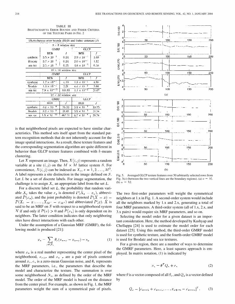
Fig. 5. Averaged GLCP texture features over 50 arbitrarily selected rows fromFig. 3(c) (between the two vertical lines are the boundary regions). (a) n = 16.(b) n = 32.

The two first-order parameters will weight the symmetricalneighbors at 1.x in Fig. 1. A second-order system would includeall the neighbors marked by 1.x and 2.x, generating a total offour MRF parameters. A third-order system (all of 1.x, 2.x, and3.x pairs) would require six MRF parameters, and so on.

Selecting the model order for a given dataset is an impor-tant consideration. Here, the method developed by Kashyap andChellappa [24] is used to estimate the model order for eachdataset [25]. Using this method, the third-order GMRF modelis used for synthetic texture, and the fourth-order GMRF modelis used for Brodatz and sea ice textures.

For a given region, there are a number of ways to determinethe GMRF parameters. Here, a least squares approach is em-ployed. In matrix notation, (1) is indicated by

(2)

where is a vector composed of all , and is a vector definedby

(3)


(a)

(b)

Fig. 6. Averaged GMRF model parameters over 50 arbitrarily selected rows from Fig. 3(c) (between the two vertical lines are the boundary regions). (a) n = 16.(b) n = 32.

The least square estimation of the parameters is evaluated by

(4)

For every pixel in a given window defined by , a is deter-mined. Then, for every window, a is estimated that providesthe GMRF features for that window.

The approach of model-based image segmentation is toarticulate the regularities between neighboring pixels mathe-


Fig. 7. Estimated texture parameters of pixel s using a 5� 5 window shouldbe more similar to the parameters of texture B than A.

(a) (b)

(c) (d)

Fig. 8. Segmentation (using n = 16) of Brodatz texture image witha three-cycle per image texture boundary. (a) Original image. (b) Truesegmentation. (c) GLCP result. (d) GMRF result.

matically, and then to exploit this information in a Bayesianframework to indicate which label has the highest probability.During the segmentation process, the prior distribution modelsare needed to capture the tendencies and constraints thatcharacterize the scenes of interest. This method will inherentlyencourage nearest neighbor pixels to have a higher probabilityof belonging to the same class.

For the segmentation problem, image is composed of twocomponents, namely a pixel intensity array and a corresponding

(a) (b)

(c) (d)

(e) (f)

Fig. 9. Segmentation of Brodatz texture image with an 11-cycle per imagetexture boundary. (a) Original image. (b) True segmentation. (c) GLCP result(n = 16). (d) GMRF result (n = 16). (e) GLCP result (n = 8). (f) GMRFresult (n = 8).

texture label array, i.e., . A Bayesian model isused to describe the probability of a certain label for a pixelgiven the pixel intensity. The iterated conditional mode (ICM)method is used to perform the GMRF image segmentation [26].For succinctness, details of this procedure are not detailed here.Further details of the MRF models and Bayesian segmentationprocedure are found in [25]. Briefly, the segmentation proceedsin two stages. First, the GMRF parameters must be estimated.This must be done because the GMRF parameters are depen-dent on the image data assigned to a particular label, and thisinformation is unknown a priori. So, to estimate the GMRF pa-rameters, the image is divided into nonoverlapping windows.For each window, the GMRF parameters are determined using(4). Then, -means is used to group like estimates and producean estimate for a given label. Second, image pixels are assignedto a particular label based on a Gibbs estimate. The estimate isbased on a Gaussian component (requiring the local image data)and a label term (based on the neighborhood label assignments).This is performed in an iterative fashion (over each pixel in theimage) until a stopping criteria or some minimum energy crite-rion is met.


III. RESEARCH QUESTIONS

The GLCP method is the preferred method for texturefeature extraction for SAR sea ice imagery [1], [3], [27].However, to obtain an optimal solution, exhaustive combinationsof quantizations, displacements, window sizes, orientations,and statistics must be performed. Brodatz imagery is oftenused as a test base for texture analysis algorithms in theresearch literature. Encouraging results have been obtainedfor unsupervised texture segmentation using Brodatz textures[28], [29]. Unfortunately, the texture appearance of a consistentice type is not as regular as a Brodatz texture, and most of thetime, different ice types as well as open water are interwovenwith each other. Can GMRF methods be used in SAR sea iceimage segmentation? Which of GLCP and GMRF producea better segmentation result? There exists limited publishedresearch investigating the potential of GMRF methods in SARsea ice image segmentation. Although many efforts consider thesupervised classification potential of GLCPs, limited researchinvestigating its unsupervised segmentation potential are known.

An important aspect of texture segmentation (using GLCPsor GMRFs) is the window coverage. Large windows producebetter estimates of the texture; however, in the case of segmenta-tion, large windows can also lead to the undesirable situation ofmultiple texture classes within a common window. Small win-dows are less likely to contain multiple classes; however, thelimited coverage may produce misleading features. These is-sues are investigated within the context of the following researchquestions.

A. Research Questions

1) Influence of Window Size: How does window size influ-ence the estimated individual GLCP texture features and GMRFmodel parameters?

The same window size ( ) can be used to determine the GLCPtexture features as well as the GMRF model parameters. Forboth methods, the size of is a very important parameter, and adifferent number of pixels in can generate different estimationresults. It is necessary to evaluate the effect of window size onthe stability of each estimated GLCP texture feature and GMRFmodel parameter. Conclusions with regard to this research ques-tion can assist the selection of a suitable window size for eachmethod.

2) Cluster Separability: How does the window size influ-ence the separability of the clusters of the estimated GLCP tex-ture features and GMRF model parameters?

This research question compares GLCP texture featuresversus GMRF model parameters for feature space separability.For a given pair of textures, the feature space separabilityfor each of GLCP and GMRF features provides a means toevaluate their texture identification ability. This evaluation willact as a basis to help understand the cause of an ineffectivesegmentation, presented later in the paper.

From this second research question, another issue can alsobe addressed, i.e., given a sufficiently large window size, whichmethod is better at characterizing texture? The question is in-spired by the fundamental difference of statistical-based and

(a) (b)

(c) (d)

(e) (f)

Fig. 10. Segmentation of Brodatz texture image. (a) Original image. (b) Truesegmentation. (c) GLCP result (n = 16). (d) GMRF result (n = 16). (e) GLCPresult (n = 32). (f) GMRF result (n = 32).

model-based texture analysis techniques. MRF texture modelsare associated with the natural formation process of the ana-lyzed textures. The model-based texture analysis technique isable to describe and reconstruct image textures. But, there is noknown method to synthesize textures based on the GLCP texturefeatures. From this point, it is a logical inference that the MRFmethod is expected to contain more complete texture structureinformation for distinguishing various textures than the GLCPmethod.

3) Multiple Textures and Irregular Boundaries: Given awindow, what is the effect on the estimated GLCP texturefeatures and GMRF model parameters if the window containsmultiple textures with the possibility of irregular boundaries?

The first and second research questions deal with homoge-neous texture samples. For the segmentation problem, some ofthe selected texture samples will contain multiple textures. Thelarger a window, the greater the probability that various classeswill be included in it. In this case, the estimation of GLCPtexture features or GMRF model parameters may be damaged.What is the relationship of the estimated texture features fromthe multitexture window with the texture features of each tex-ture in the window?


IV. METHODS AND TESTING

A. Research Question 1: Influence of Window Size

1) Method for Research Question 1: Influence of WindowSize: How does the window size influence the estimated indi-vidual GLCP texture features and GMRF model parameters?

For a given texture, the relative change of a feature’s stan-dard deviation as a function of window size is calculated. Theexperiment is designed to check the effect of different windowsizes on the stability of the estimation in each dimension foreach method.

One synthetic texture (1024 1024) [generated using themodel parameters “A” in Table I and illustrated in Fig. 2(a)]one Brodatz texture (1024 1024) (pigskin) (illustrated onthe right-and side of Fig. 3(b), and one SAR sea ice image(768 768) [the multiyear component of Fig. 2(c)] are usedfor the experiments. The SAR image, as obtained from theCanadian Ice Services (CIS), was captured from the BeaufortSea, October 13, 1997, using Radarsat ScanSAR SW1 mode(2 2 block averaged to 100-m pixels). Note that the SARimages used in this paper have accompanying operational icecharts produced at CIS. This information is used to deter-mine ice types in the imagery. From each texture image, 60window samples are randomly selected for each window size( ). The standard deviation per featureper window size is determined for each set of 60 samples. Tomeasure the relative change, the value of is normalized bythe of the 96 window size for a given feature.

2) Results for Research Question 1: Influence of WindowSize: Representative plots are provided in Fig. 4 using thepigskin texture of Brodatz image (each dataset producedsimilar results). These plots show relative changes of foreach estimated GLCP texture feature and each GMRF modelparameter from window size 96 to window size 8. Fig. 4(a)plots six representative GLCP texture features, and Fig. 4(b)plots the six third-order GMRF model parameters. A pair ofobservations are noted. First, larger windows lead to morestable texture features estimates than smaller windows. Sim-ilarly, with decreasing window size, the of each estimatedGLCP texture feature and the GMRF model parameter increaseexponentially. Second, with decreasing window size, the ofeach GMRF model parameter increases faster than the GLCPtexture features, especially from window size 32 to windowsize 8.

These observations are supported by the values in Table II,which indicates the average standard deviation ratios of eachestimation from all three textures used in this experiment. Forexample, using the GLCP method, the largest average standarddeviation ratio is 9.33 using a synthetic texture based on com-paring window sizes 8–96, whereas, the largest ratio using theGMRF method is 28.32, which also occurred using the synthetictexture and the window size 8 compared to 96. The GMRF’saverage standard deviation ratio of the smaller window sizes(64, 32, 16, 8) to the larger window size (96) always exceedsthat of the GLCPs. Positive and negative values of the GMRFmodel parameter behave quite differently in the texture forma-tion process. In this case, large standard deviations could signif-icantly damage the texture model estimation.

(a) (b)

(c) (d)

(e) (f)

Fig. 11. Segmentation of Brodatz texture image. (a) Original image. (b) Truesegmentation. (c) GLCP result (n = 16). (d) GMRF result (n = 16). (e) GLCPresult (n = 32). (f) GMRF result (n = 32).

Based on this experiment, to obtain a stable estimation, theGMRF method requires a relatively larger window size than theGLCP to obtain the same degree of stability in the feature esti-mates. It is noted here that textures are generally multiscale andmay require the use of more than one window size to performsegmentation properly. For brevity, only the relative ability ofthe GLCP and GMRF methods will be investigated in this paper.

B. Research Question 2: Cluster Separability

How does the window size influence the separability of theclusters of estimated GLCP texture features and GMRF modelparameters?

1) Method for Research Question 2: Cluster Separa-bility: This research question explores the effect of differentwindow sizes on the multidimensional feature space separa-bility. The Fisher criterion [20] is used as a nonparametricmeasure of the separability of two class clusters in the featurespace. This criterion calculates a ratio of the between-classseparability and the within-class variation. Larger Fisher cri-terion values demonstrate improved separation of two classes.Further insight can be obtained by calculating the upper boundof classification error between feature cluster pairs using theBhattacharyya error bound [20]. In this case, smaller errors


Fig. 12. GLCP segmentation result for STAR-1 image.

indicate better separability of two class clusters in the featurespace.

Three texture image pairs are used for testing, as illustratedin Fig. 2. These include synthetic (1024 1024) (models A andB in Table I), Brodatz (1024 1024) (wood grain and raffia),and SAR sea ice texture images (768 768). The multiyear iceis obtained from the same image used in Research Question 1.The first-year sample uses the same modality and processingbut was captured from the Gulf of St. Lawrence on February 191997. Sixty sample windows with sizes 8, 16, 32, and 64 arerandomly selected from each image. The two images in eachpair represent internally consistent but mutually distinct texturepatterns.

2) Results for Research Question 2: Cluster Separa-bility: Table III reports the Bhattacharyya error bounds(BEBs) of each texture pair and the Fisher criterion ( ) of eachprojected texture pair. A number of observations can be made.When , all of the GLCP pairs have a lower Bhattacharyyabound as well as a higher Fisher criterion compared to theGMRF pairs. In contrast, for and , the GMRFhas lower Bhattacharyya bound and higher Fisher criterion.Separability is relatively strong given smaller windows forGLCP texture features compared to GMRF texture features.However, for large windows, GMRF features are more sepa-rable than GLCP features. Corresponding line projections (forsuccinctness, these are not displayed here) visibly validate

Fig. 13. GMRF segmentation result for the STAR-1 image.

these numerical results. Testing for produces similarresults as for .

Based on this experiment, another conclusion in the secondresearch question can be obtained. With a large window size,the GMRF model and GLCP texture features have capable sep-arability given homogeneous samples. The BEBs are all at moston the order of , indicating that the homogeneous 32 32windows contain sufficient data to distinguish the given classpairs.

C. Research Question 3: Multiple Textures and IrregularBoundaries

Given a window, what is the effect on the estimated GLCPtexture features and GMRF model parameters if the windowcontains multiple textures with the possibility of an irregularboundary?

1) Method for Research Question 3: Multiple Texturesand Irregular Boundaries: Features for windows containingmultiple textures can produce misleading segmentation results.Based on the calculation of GLCP texture features and GMRFmodel parameters, a reasonable assumption is that the extractedGLCP or GMRF texture features from a multitexture windowshould have a linear weighting proportional to the area coverageof individual texture features. For example, given two texturetypes A and B in window , then , where

is any texture feature of window , is the area proportion


Fig. 14. GLCP segmentation result for Radarsat image captured over the Gulfof St. Lawrence (February 19, 1997).

of texture A in window , is the area proportion of texture Bin window , and .

2) Results for Research Question 3: Multiple Textures andIrregular Boundaries: Fig. 3(a)–(c) shows three bipartite tex-ture images, each 256 256: synthetic, Brodatz, and SAR seaice, respectively. Texture estimates for each image are estimatedbased on two window sizes ( , ) for samples cen-tered at each pixel across 50 randomly selected rows. Selectedresults are only presented for the sea ice image [Fig. 3(c)] be-cause results for other images are similar in nature. Figs. 5 and6 depict the average feature values for the 50 samples for eachof GLCP and GMRF texture features, respectively. The verticalline pairs represent the window extent when centered on theboundary of the two textures. The resulting parameters changein approximately a linear manner from one texture to another.

This experiment demonstrates that texture measures usingeither method can be damaged by the multitexture windows.Given a window with multiple textures, each estimated GLCPtexture feature seems to be a weighted linear combination of thecorresponding GLCP texture features of each texture. The sameconclusion applies to each estimated GMRF model parameter.

Consequently, significant segmentation error can occur, as il-lustrated by Fig. 7. The boundary between textures A and B is aright angle. Nine pixels in a 5 5 window are located on pixel ,and 16 pixels belong to texture B. Pixel belongs to texture A.

Based on the above experiment, for both methods, the derivedfeatures will be closer to texture B than to texture A, encour-aging pixel to be misclassified as texture B. In this case, thecorner pixel would be eroded, since it would be erroneouslyclassified as texture B. This example illustrates that textured im-ages with irregular boundaries will strongly affect the perfor-mance of the texture segmentation methods. Commonly, texturefeature images in the research literature utilize straight bound-aries, which can provide misleading results if extrapolated tonatural imagery with irregular texture boundaries.

How do these damaged estimations affect the segmentationresults for each method? Figs. 8 and 9 show the segmentationresults of two bipartite images with different texture boundaries.To concentrate on the effect of the textural boundary on the seg-mentation, each image contains the same two Brodatz textures(paper and pigskin). In the case of a straight vertical boundarygiven both and , GLCP and GMRF texture fea-tures and their associated segmentation schemes successfullysegment the image (not shown for brevity).

Fig. 8(a) has a sinusoidal boundary with three periods, whichmakes it difficult to distinguish compared to a straight boundary.For each GLCP and GMRF, a 16 16 window size is used,and the segmentation result is effective. By increasing the fre-quency of the sinusoidal boundary, a more difficult segmenta-tion problem is produced (see Fig. 9). The segmentation resultsfor both GLCP and GMRF using a 16 16 window are unsuc-cessful [see Fig. 9(c) and (d)]. Fig. 9(e) and (f) shows the seg-mentation results using an 8 8 window size. In this case, theGLCP method produces a much better segmentation than theGMRF method. Also, generates a much better result than

, given the GLCP texture features.For multiple texture images with simple boundaries, sample

windows will contain single textures more often than such im-ages with complex boundaries. For simple boundaries, both theGLCP and GMRF methods can produce correct feature esti-mates, which leads to an accurate segmentation. For complexboundaries, both methods may have damaged features estimatesthat can erode the quality of the segmentation. To minimize theeffect of multiple texture windows, small windows should beused. In such cases, the GLCP method should be employed, assupported by the first two research questions.

D. Image Segmentation Results

In this section, the GLCP and GMRF methods will be ap-plied to the segmentation of two Brodatz and three SAR seaice images. Note that the Brodatz images contain boundariesthat are simple relative to the boundaries found in SAR seaice imagery. The first example is a three-class Brodatz image[Fig. 10(a)]. The true segmentation is illustrated in Fig. 10(b).Given a window size of , GLCPs [Fig. 10(c)] are betterable to segment the image than GMRFs [Fig. 10(d)]. Whenthe window size is increased to , GMRFs generatea marginally better segmentation [Fig. 10(f)] than the GLCPs[Fig. 10(e)]. Both methods produce improved segmentationswhen the window size is increased; however, the relative im-provement for the GMRF method is significant. The GMRFmethod requires a larger spatial extent to estimate the model


Fig. 15. GMRF segmentation result for a Radarsat image captured over theGulf of St. Lawrence (February 19, 1997).

Fig. 16. GLCP segmentation result for a Radarsat image captured over theBeaufort Sea (October 13, 1997).

parameters and perform an accurate segmentation. Also, for

Fig. 17. GMRF segmentation result for a Radarsat image captured over theBeaufort Sea (October 13, 1997).

, the GMRF method has a better approximation for thecurved boundary.

The second Brodatz image [Fig. 11(a)] contains four tex-tures separated by horizontal and vertical sinusoidal boundaries.Once again, the larger window size ( ) allows the GMRFmethod to produce a reasonable image segmentation [Fig. 11(f)]compared to a window size of [Fig. 11(d)]. The GLCPsare not able to properly identify the boundary region betweenthe textures [Fig. 11(c) and (e)]. The GMRF segmentation pro-cedure produces a superior result for this case. The GMRF seg-mentation process is advantageous because it uses a label imagemodel that encourages neighbor pixels to be assigned to thesame class.

From the earlier testing using different window sizes (seeTable II), one can see that both methods prefer a larger windowsize to obtain a robust estimation. But, the larger window sizemay cause a segmentation problem using the GLCP method inthe boundary area, i.e., the true boundary between textures maybe blurred, and sometimes, the pixels along the boundary areascould be misclassified as another texture class. To overcomethis boundary problem, the window size should be as small aspossible for the GLCP method. Using the GMRF method, sucha small window size may compromise the quality of the tex-ture features. As a result, the GMRF window size should beas large as possible. As discussed previously, given complextexture boundaries, a large window could also damage the es-timated parameters.

The last three segmentation results are based on SAR seaice images. Because the sea ice texture has a finer appearancethan Brodatz textures, for these images, the window size usedin the GLCP method is 13 13, and the window size used inthe GMRF method is 16 16. The full sea ice image presentedin Figs. 12 and 13 was first published in [31]. The image is


a STAR-1 X-HH image (6-m resolution). Here, a 336 466subimage of the full image is used. Two ice types are identified:first-year ice and multiyear ice. Both methods can distinguishthe two ice types. The boundaries generated from the GMRFmethod are more accurate than the GLCP method. Visually ob-serving the boundary locations in these two figures, one can seethat the edges determined by the GMRF method present moreappropriately the boundaries of different ice types. However, theGMRF method has problems to properly discriminate the mul-tiyear ice in the floes close to the bottom of the image.

The second SAR sea ice image is a Radarsat ScanSAR SW1C-band HH image obtained from CIS. The pixel spacing is100 m (2 2 block averaged), and the image size is 495 669.The scene was captured over the Gulf of St. Lawrence on Feb-ruary 19, 1997, in a descending orbit. The image segmentationsare found in Figs. 14 (GLCP) and 15 (GMRF). Both methodsare readily able to perform the segmentation; however, theGMRF method has relatively better boundary approximations.Many of the thin first-year ice regions separating the multiyearfloes are not recognized, due to poor features estimates forsuch regions.

The third sea ice image was also obtained from CIS. Theimage has the same parameters as the previous SAR image;however, this image was obtained October 13, 1997, in an as-cending orbit over the Beaufort Sea and is 486 486. Edgemaps are displayed in Figs. 16 (GLCP) and 17 (GMRF), andregion maps are displayed in Figs. 18 (GLCP) and 19 (GMRF).Such a SAR image illustrates a more difficult task for an au-tomated segmentation algorithm for operational ice reconnais-sance. Multiyear ice, new ice, and gray ice are contained in theimage. The new ice (dark tone) can be found in the middle ofthe image. Gray ice is found in the top and bottom regions of theimage. The multiyear ice floes with a brighter tone than gray iceare mingled with the gray ice and can be found primarily in thetop region.

The GLCP method and GMRF methods generate differentsegmentation results, and both methods do not perform aswell as the first two SAR images. Generally speaking, theGLCP method generates a better segmentation image thanGMRF method. The GMRF method tends to underrepresentthe amount of new ice, confusing it with gray ice. Relatively,the GLCP segmentation generates a better segmentation ofthe new ice region. In distinguishing multiyear ice and grayice, the two methods have a different tendency. The GMRFmethod is unable to properly capture locally uniform texturecharacteristics, and the segmentation result appears morediscontinuous than GLCP method. The GLCP method tendsto confuse the multiyear ice with gray ice on the top region ofthe image, delineating the gray ice more than it should. Notethat the human observer would tend to identify the gray icein the bottom left as gray ice, due to the nature of the shapeof the leads in that region. Younger ice (such as gray ice)tends to produce leads with the observed characteristic shapes,providing an additional basis for manual ice classification.

Comparing the three ice images, one can notice that the pat-tern of each ice type in the first two SAR images is more ac-curately defined than the pattern in the third image. Also, the

Fig. 18. GLCP segmentation result with regions identified for a Radarsatimage captured over the Beaufort Sea (October 13, 1997).

Fig. 19. GMRF segmentation result with regions identified for a Radarsatimage captured over the Beaufort Sea (October 13, 1997).

texture patterns of the ice types in the first two images have amore visually distinct difference than those in the third image.Finally, the multiyear ice and gray ice in the third SAR imagehave considerable mixing, leading to each having smaller localimage extent. All of these could result in a poorer model estima-tion and make the third image more difficult to segment usingthe GMRF method. It is possible that the pixel resolution of theRadarsat image (100 m) contributes to the poorer segmentation


result relative to the STAR-1 image (6-m resolution). Opera-tionally, it is more cost-effective to utilize the Radarsat imagery,and algorithms should be developed in support of this platform.

V. SUMMARY

There exists a lack of published research comparing unsuper-vised texture segmentation methods. Gray-level cooccurrenceprobabilities and Gaussian Markov random fields are two pop-ular texture methods. GLCPs are commonly applied to remotesensing imagery in the research literature, while GMRFs havenot been used extensively for this purpose. The goal of this paperwas to develop a better understanding of the ability of eachmethod in the unsupervised segmentation of SAR imagery byconsidering the role of window size in the segmentation process.

A number of research questions were posed and studied,producing the following results. GMRFs require increasedwindow sizes relative to GLCPs to produce stable textureestimates. GLCPs produce more separable texture features forsmaller windows than the GMRF texture features. Across threedifferent datasets (synthetic, Brodatz, and SAR), a windowsize of 32 was deemed sufficiently large to obtain separable,consistent texture features. However, such a large window sizecan lead to segmentation error due to the higher risk of multipleclasses appearing in the same window. Given a window withmultiple textures, a linear weighting of the ratio of the texturesin the image generates the overall texture feature. Such aweighting can lead to erroneous boundary delineation and caneven misclassify the boundary itself as an incorrect class. Thesegmentation of classes separated by irregular boundaries foundin remote sensing imagery will be affected by this problem. Thetexture literature often utilizes convenient texture boundaries,yet complex boundaries, coupled with varying local classspatial extents, pose greater challenges to the operational useof image segmentation algorithms.

ACKNOWLEDGMENT

This work is part of an ongoing collaboration with CIS(http://www.cis.ec.gc.ca/home.html). CIS is thanked for en-couragement as well as the provision of data. The authorsappreciate the assistance of M. Arkett, R. De Abreu, D. Flett,M. Manore, B. Ramsay, and K. Wilson. Thanks to the anony-mous reviewers, whose helpful advice improved the quality ofthe manuscript.

REFERENCES

[1] Q. A. Holmes, D. R. Nuesch, and R. A. Shuchman, “Textural analysisand real-time classification of sea-ice types using digital SAR data,”IEEE Trans. Geosci. Remote Sensing, vol. GE-22, pp. 113–120, Mar.1984.

[2] M. E. Shokr, “Evaluation of second-order texture parameters for sea iceclassification from radar images,” J. Geophys. Res., vol. 96, no. C6, pp.10 625–10 640, 1991.

[3] D. G. Barber and E. F. LeDrew, “SAR sea ice discrimination usingtexture statistics: A multivariate approach,” Photogramm. Eng. RemoteSens., vol. 57, no. 4, pp. 385–395, 1991.

[4] M. Tuceryan and A. K. Jain, “Texture analysis,” in Handbook of Pat-tern Recognition and Computer Vision, C. Chen, L. Pau, and P. Wang,Eds. Singapore: World Scientific, 1993, ch. 2.1, pp. 235–276.

[5] R. M. Haralick, K. Shanmugam, and I. Dinstein, “Textural features forimages classification,” IEEE Trans. Syst., Man Cybern., vol. 3, no. 6, pp.610–621, 1973.

[6] J. E. Besag, “Spatial interaction and the statistical analysis of lattice sys-tems (with discussion),” J. R. Statist. Soc. B, vol. 36, no. 2, pp. 192–236,1974.

[7] A. K. Jain and F. Farrokhnia, “Unsupervised texture segmentation usingGabor filters,” Pattern Recognit., vol. 24, no. 12, pp. 1167–1186, 1991.

[8] D. A. Clausi and M. E. M. E. Jernigan, “Establishing Gabor filter param-eters for optimal texture separability,” Pattern Recognit., vol. 33, no. 11,pp. 1835–1849, 2000.

[9] T. Randen and J. H. Husoy, “Filtering for texture classification: A com-parative study,” IEEE Trans. Pattern Anal. Machine Intell., vol. 21, pp.291–310, Apr. 1999.

[10] P. Brodatz, Textures: A Photographic Album for Artists and De-signers. New York: Dover, 1966.

[11] O. Pichler, A. Teuner, and B. J. Hosticka, “A comparison of texture fea-ture extraction using adaptive Gabor filtering, pyramidal and tree struc-tured wavelet transforms,” Pattern Recognit., vol. 29, no. 5, pp. 733–742,1996.

[12] T. Ojala, M. Pietikainen, and D. Harwood, “A comparative study of tex-ture measures with classification based on feature distributions,” PatternRecognit., vol. 29, no. 1, pp. 51–59, 1996.

[13] P. P. Ohanian and R. C. Dubes, “Performance evaluation for four classesof textural features,” Pattern Recognit., vol. 25, no. 8, pp. 819–833,1992.

[14] R. W. Conners and C. A. Harlow, “Theoretical comparison of texturealgorithms,” IEEE Trans. Pattern Anal. Machine Intell., vol. PAMI-2,pp. 204–222, May 1980.

[15] J. S. Weszka, C. R. Dyer, and A. Rosenfeld, “A comparative study oftexture measures for terrain classification,” IEEE Trans. Syst., Man Cy-bern., vol. 6, no. 4, pp. 269–285, 1976.

[16] J. R. Carr and F. P. dc Miranda, “The semivariogram in comparison to theco-occurrence matrix for classification of image texture,” IEEE Trans.Geosci. Remote Sensing, vol. 36, pp. 1945–1952, Nov. 1998.

[17] P. Gong, D. J. Marceau, and P. J. Howarth, “A comparison of spatialfeature extraction algorithms for land-use classification with SPOT HRVdata,” Remote Sens. Environ., vol. 40, pp. 137–151, 1992.

[18] D. A. Clausi, “Comparison and fusion of co-occurrence, Gabor andMRF texture features for classification of SAR sea-ice imagery,”Atmos.-Ocean, vol. 39, no. 3, pp. 183–194, 2001.

[19] , “An analysis of co-occurrence texture statistics as a function ofgrey level quantization,” Can. J. Remote Sens., vol. 28, no. 1, pp. 45–62,2002.

[20] R. O. Duda, P. E. Hart, and D. G. Stork, Pattern Classification. NewYork: Wiley, 2001.

[21] R. Chellappa and S. Chatterjee, “Classification of texture usingGaussian Markov random fields,” IEEE Trans. Acoust., Speech, SignalProcessing, vol. ASSP-33, pp. 959–963, Aug. 1985.

[22] F. S. Cohen, Z. Fan, and M. A. Patel, “Classification of rotated and scaledtexture images using Gaussian Markov random fields,” IEEE Trans. Pat-tern Anal. Machine Intell., vol. 13, pp. 192–203, Feb. 1991.

[23] S. Geman and C. Graffigne, “Markov random field image models andtheir applications to computer vision,” in Proc. Int. Congr. Mathemati-cians, 1986.

[24] R. L. Kashyap and R. Chellappa, “Estimation and choice of neighborsin spatial-interaction models of images,” IEEE Trans. Inform. Theory,vol. 29, no. 1, pp. 61–72, 1983.

[25] B. Yue, “SAR sea ice recognition using texture methods,” Master’sthesis, Univ. Waterloo, Waterloo, ON, Canada, 2001.

[26] J. Besag, “On the statistical analysis of dirty pictures,” J. R. Statist. Soc.B, vol. 48, pp. 259–302, 1986.

[27] L. K. Soh and C. Tsatsoulis, “Texture analysis of SAR sea ice imageryusing gray level co-occurrence matrices,” IEEE Trans. Geosci. RemoteSensing, vol. 37, pp. 780–795, Mar. 1999.

[28] B. S. Manjunath and R. Chellappa, “Unsupervised texture segmentationusing Markov random field models,” IEEE Trans. Pattern Anal. MachineIntell., vol. 13, pp. 478–482, May 1991.

[29] H. Derin and W. S. Cole, “Segmentation of textured images using Gibbsrandom fields,” Comput. Vis., Graph. Image Process., vol. 35, pp. 72–98,1986.

[30] S. Krishnamachari and R. Chellappa, “Multi-resolution Gauss-Markovrandom field models for texture segmentation,” IEEE Trans. Image Pro-cessing, vol. 6, pp. 251–267, Feb. 1997.

[31] D. G. Barber, M. E. Shokr, R. A. Fernandes, E. D. Soulis, D. G. Flett,and E. F. LeDrew, “A comparison of second-order classifiers for SARsea ice discrimination,” Photogramm. Eng. Remote Sens., vol. 59, no. 9,pp. 1397–1408, 1993.


David Clausi (S’93–M’96–SM’03) received theB.A.Sc., M.A.Sc., and Ph.D. degrees from theUniversity of Waterloo, Waterloo, ON, Canada, in1990, 1992, and 1996, respectively.

From 1996 to 1997, he worked in the medicalimaging field with Mitra Imaging, Inc., Waterloo.From 1997 to 1999, he was an Assistant Professorin the Department of Geomatics Engineering,University of Calgary, Calgary, AB, Canada. In1999, he returned to the University of Waterloo andis currently an Associate Professor in the Systems

Design Engineering program. His research interests include automatedimage interpretation, digital image processing, and pattern recognition withapplications in remote sensing and medical imaging.

Bing Yue received the undergraduate degree inelectrical engineering from Hebei University ofTechnology, Tianjin, China, in 1991, and theM.A.Sc. degree in systems design engineering fromthe University of Waterloo, Waterloo, ON, Canada,in 2001.

From 1991 to 1999, she was an Engineer withthe Remote Sensing Geology Department, ResearchInstitute of Petroleum Exploration and Development,Beijing, China. Since 2002, she has been a ResearchAssistant with Noetix Research Inc., Ottawa, ON,

under contract with the Canada Center for Remote Sensing, Ottawa. Hercurrent research interests include remotely sensed digital image processing,target detection, SAR polarimetry, interferometry, and pattern recognition.

ieee transactions on geoscience and …dclausi/papers/published 2004/clausi and yue...random fields...

Documents