1

IEEE P1159.1

Guide For Recorder and Data Acquisition Requirements For Characterization of Power Quality Events

Draft 0.1

February 19, 2000

Copyright © 2000 by the Institute of Electrical and Electronic Engineers, Inc. 345 East 47th Street

New York, NY 10017, USA All rights reserved.

This is an unapproved draft of a proposed IEEE Standard, subject to change. Permission is hereby granted for IEEE Standards Committee participants to reproduce this document for purposes of IEEE standardization activities. Permission is also granted for member bodies and technical committees of ISO and IEC to reproduce this document for purposes of developing a national position. Other entities seeking permission to reproduce this document for these or other uses must contact the IEEE Standards Department for the appropriate license. Use of information contained in this unapproved draft is at your own risk.

IEEE Standards Department Copyright and Permissions

445 Hoes Lane, P.O. Box 1331 Piscataway, NJ 08855-1331, USA

2

3

Table of contents

1. Overview ........................................................................................................... 4

1.1 Scope............................................................................................................................4

1.2 Purpose........................................................................................................................4

2. References: ....................................................................................................... 4

3. Definitions ........................................................................................................ 4

4. Application classes.......................................................................................... 11

4.1 Class A, reference performance ...................................................................................12

4.2 Class B, indicator performance....................................................................................12

5. Input voltage and current requirements ......................................................... 12

5.1 Transients ..................................................................................................................13

5.2 Short duration variations ..........................................................................................15

5.3 Long-duration variations...........................................................................................17

5.4 Voltage unbalance......................................................................................................18

5.5 Waveform distortion .................................................................................................19

5.6 Voltage fluctuations......................................................................................................22

5.7 Power Frequency variations......................................................................................22

6. Performance test and calibration procedures ................................................. 23

6.1 Accuracy tests ..................................................................................... 23 7. Bibliography ................................................................................................... 25

4

1. Overview

1.1 Scope

This guide establishes the data acquisition attributes necessary to characterize the electromagnetic phenomena.

1.2 Purpose

The objective of this guide is to describe the technical measurement requirements for each type of disturbance defined in 24 categories of typical characteristics of power system electromagnetic phenomena. Each category is discussed in several standards in terms of emission limits, severity levels, planning levels or immunity levels.

2. References:

(to be accumulated by each chapter chair)

3. Definitions

Note: Definitions given in this section have not been harmonized with definitions made in other IEEE standards. Several terms need to be defined, however, and IEEE 1159.1 seeks volunteers for the harmonizing of definitions.

When the signal to measure is supplied from a perfectly stable waveform generator, results displayed by one instrument may be very close to those obtained by others. However, when connected to the power system, several phenomena can affect the measurement in such a way that some instruments can record disturbance levels that do not exist and several errors can be added to the remaining harmonics assessed.

Without the assessment specification of the instrument, or with an inappropriate specification, users are unable to assess the severity level of the disturbance on equipment; this can lead to incorrect conclusions and costly decisions. Users should ask manufacturers for the complete measurement-instrument specification, this may include the following information:

• sampling rate, • bandwidth amplitude/frequency • accuracy (the instrument should stay within the limits 100% of the time) • precision (the instrument should stay within the limits 68.27% of the time) • resolution (signal-to-noise ratio or effective bits)

5

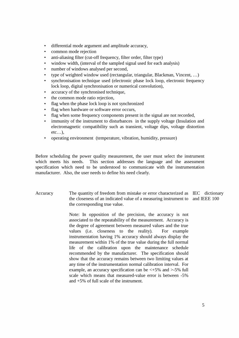
• differential mode argument and amplitude accuracy, • common mode rejection • anti-aliasing filter (cut-off frequency, filter order, filter type) • window width, (interval of the sampled signal used for each analysis) • number of windows analysed per second, • type of weighted window used (rectangular, triangular, Blackman, Vincent, … ) • synchronisation technique used (electronic phase lock loop, electronic frequency

lock loop, digital synchronisation or numerical convolution), • accuracy of the synchronised technique, • the common mode ratio rejection, • flag when the phase lock loop is not synchronized • flag when hardware or software error occurs, • flag when some frequency components present in the signal are not recorded, • immunity of the instrument to disturbances in the supply voltage (Insulation and

electromagnetic compatibility such as transient, voltage dips, voltage distortion etc… ),

• operating environment (temperature, vibration, humidity, pressure)

Before scheduling the power quality measurement, the user must select the instrument which meets his needs. This section addresses the language and the assessment specification which need to be understood to communicate with the instrumentation manufacturer. Also, the user needs to define his need clearly.

Accuracy The quantity of freedom from mistake or error characterized as the closeness of an indicated value of a measuring instrument to the corresponding true value.

Note: In opposition of the precision, the accuracy is not associated to the repeatability of the measurement. Accuracy is the degree of agreement between measured values and the true values (i.e. closeness to the reality). For example instrumentation having 1% accuracy should always display the measurement within 1% of the true value during the full normal life of the calibration upon the maintenance schedule recommended by the manufacturer. The specification should show that the accuracy remains between two limiting values at any time of the instrumentation normal calibration interval. For example, an accuracy specification can be <+5% and >-5% full scale which means that measured-value error is between -5% and +5% of full scale of the instrument.

IEC dictionary and IEEE 100

6

Aliasing The distortion caused by sampling a signal at an inappropriate rate and which results in the overlapping of the sidebands around the harmonics of the sampling frequency in the spectrum of the sample signal.

Note: A high frequency which exceeds the operating range of the instrument affects the frequency component in the frequency range of the analysis. IEC has requested use of an anti-aliasing filter which should attenuate to below 50 dB all frequencies above the operating range of the instrument. Observation windows may be flagged during the presence of frequency components which exceed the operating range of the instrument. If these high frequency components occur too often, the user may need a wider bandwidth instrument to capture the actual signal to measure.

IEC dictionary

Analogue signal

A signal in which the characteristic quantity representing information may, at any instant, assume any value within a continuous interval.

Note. For example, an analogue signal may follow continuously the values of another physical quantity representing information

IEC dictionary

Anti-aliasing Correction intended to reduce the aliasing.

IEC dictionary

Aperture uncertainty

Signal error of the sample-hold electronic device caused by the timing uncertainty in the switch and the driver circuit.

Bandwidth The width of a frequency band over which a given characteristic of an equipment or transmission channel does not differ from a reference value by more than a specified amount or ratio. Note.: the given characteristic may, for example, be the amplitude/frequency, the phase/frequency or the delay/frequency characteristic.

The quantitative difference between the limiting frequencies of a frequency band. For most power quality users should specify

7

the bandwidth as the frequency for which the maximum sinusoidal input signal has decreased below the accuracy specified

Digital signal A discretely timed signal in which information is represented by a finite number of well defined discrete values that one of its characteristic quantities may take in time.

Dynamic accuracy

Accuracy determined for a time-varying output IEEE 100

Dynamic range The ratio, usually expressed in decibels, of the maximum to the minimum signal input amplitude over which an amplifier can operate within some specified range of performance.

IEEE 100

Effective bits Effective bits is a measure of the signal-to-noise ratio given in term of the number of bits. The signal to noise ratio is

generally expressed in decibels 10 ×

log

wanted powernoise power

of

the power of the (wanted) signal to that of the noise at the specified point under specific conditions. The noise, also called lost bits for most digital power quality monitors, includes the differential non-linearity, amplifier and digitizer noise, integral non-linearity, aperture uncertainty, phase error, sampling rate error and trigger jitters. In practice, the signal measured can be the voltage (U) or the current (I) which is related to the same circuit impedance which is also valid for the noise. Therefore, for a voltmeter or ammeter, the signal to noise ratio can be

expressed by 20 ×

log

UU

signal

noise

. The effective bits is

calculated using the following equation:

Datel1

1 Bob Leodard, “Understanding data converters’ frequency domain specifications,”

8

6.02current or the voltagethe

of amplitudeinput actual amplitude scale Full

log2076.1

+−

=

SNR

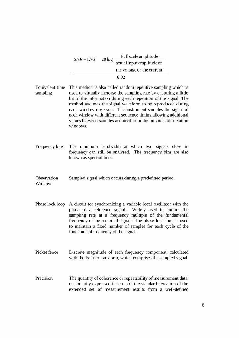
Equivalent time sampling

This method is also called random repetitive sampling which is used to virtually increase the sampling rate by capturing a little bit of the information during each repetition of the signal. The method assumes the signal waveform to be reproduced during each window observed. The instrument samples the signal of each window with different sequence timing allowing additional values between samples acquired from the previous observation windows.

Frequency bins The minimum bandwidth at which two signals close in frequency can still be analysed. The frequency bins are also known as spectral lines.

Observation Window

Sampled signal which occurs during a predefined period.

Phase lock loop A circuit for synchronizing a variable local oscillator with the phase of a reference signal. Widely used to control the sampling rate at a frequency multiple of the fundamental frequency of the recorded signal. The phase lock loop is used to maintain a fixed number of samples for each cycle of the fundamental frequency of the signal.

Picket fence Discrete magnitude of each frequency component, calculated with the Fourier transform, which comprises the sampled signal.

Precision The quantity of coherence or repeatability of measurement data, customarily expressed in terms of the standard deviation of the extended set of measurement results from a well-defined

9

(adequately specified) measurement process in a state of statistical control. The standard deviation of the conceptual population is approximated by the standard deviation of an extended set of actual measurements. When not specified, the precision specification is assumed to be repeatable during one standard deviation interval that is 68.27% of the measurements.

Note: The precision specification applied in surveying to the degree of perfection in the methods and instruments used when making measurements and obtaining results of a high order of accuracy.

Random Error (Er)

The random error is one which causes the measured value to occur randomly around an average value.

Resolution The smallest change in the measured or supplied quantity to which a numerical value can be assigned without interpolation.

Note: the resolution of most digital instruments is specified in terms of the number of bits that the analogue to digital converter can provide. Manufacturers have invented several wordings such as effective bits.

IEC dictionary

Sampling with interpolation

Method used to get an idea of what a sampled signal looks like if it is so fast that the recorder can only collect a few sample points. Linear interpolation connects sample points with straight lines, and sine interpolation connects samples with curves.

Sampled signal Signal representing a variable which is only intermittently observed and represented. The sequence of values of a signal taken at discrete instants.

Sideband The spectral components resulting from the modulation of a sinusoidal carrier and lying above or below the carrier frequency.

Note.: Sideband designates a frequency band lying above or below a sinusoidal carrier frequency and containing spectral

IEC dictionary

10

components of significance produced by modulation. Flicker originated from a lamp is produced by the modulation of the power-system voltage operated at the fundamental frequency. Thus, the fundamental frequency is the carrier frequency and the modulation produces the sidebands.

signal A measurable variable, one or more parameters of which carry information about one or more variables which the signal represents

Signal window Test signal representing a uniform background with a uniform rectangular or square area, clearly contrasted in relation to the background

IEC

Spectral leakage

Frequency component of a spectrum resulting from a signal discontinuity at the boundary of the observation window. This signal discontinuity occurs when a fraction of a cycle exists in the waveform comprised in the observation window which is subjected to the Fourier transform.

Static accuracy Accuracy determined with a constant output which is independent of the time-varying nature of the variable

Time-domain instrumentation

Instrumentation which performs the analysis by time sampling of the signals and subsequent numerical handling of the sampled data. Fast Fourier Transform (FFT) is the most widely used computation algorithm for harmonic analysis

IEC1000-4-7

Mean ( x ): The mean of a number of measurements performed during a period or an interval of a given quantity is defined by

∑=

=N

iix

Nx

1

1

rms ( x~ ) The rms x~ of a number of measurements performed during a period or an interval of a given quantity is defined by

11

period or an interval of a given quantity is defined by

N

xX

N

ii∑

== 1

2

~

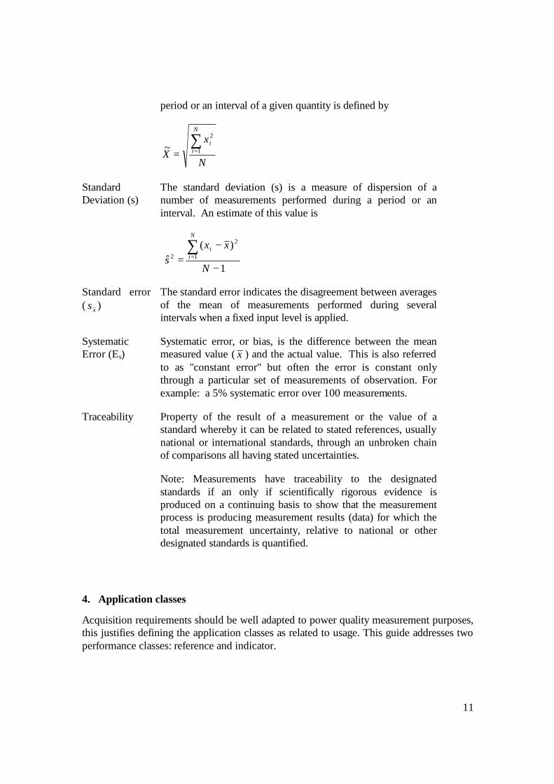
Standard Deviation (s)

The standard deviation (s) is a measure of dispersion of a number of measurements performed during a period or an interval. An estimate of this value is

1

)(ˆ 1

2

2

−

−=∑=

N

xxs

N

ii

Standard error ( xs )

The standard error indicates the disagreement between averages of the mean of measurements performed during several intervals when a fixed input level is applied.

Systematic Error (Es)

Systematic error, or bias, is the difference between the mean measured value ( x ) and the actual value. This is also referred to as "constant error" but often the error is constant only through a particular set of measurements of observation. For example: a 5% systematic error over 100 measurements.

Traceability Property of the result of a measurement or the value of a standard whereby it can be related to stated references, usually national or international standards, through an unbroken chain of comparisons all having stated uncertainties.

Note: Measurements have traceability to the designated standards if an only if scientifically rigorous evidence is produced on a continuing basis to show that the measurement process is producing measurement results (data) for which the total measurement uncertainty, relative to national or other designated standards is quantified.

4. Application classes

Acquisition requirements should be well adapted to power quality measurement purposes, this justifies defining the application classes as related to usage. This guide addresses two performance classes: reference and indicator.

12

4.1 Class A, reference performance

This category is for instruments used in application where precise measurements are necessary, e.g. verifying compliance with standards, resolving disputes, etc..

Any two instruments that comply with the requirements of Class A, when connected to the same signals, will produce matching results within the specified accuracy (or will indicate that matching is not possible).

To ensure that matching results are produced, Class A performances may require absolute time accuracy sufficient to ensure matching results.

4.2 Class B, indicator performance

Class B performance may be used for general surveys, initial diagnosis, and other applications where high accuracy is not necessarily required. Under some circumstances, the results will not necessarily match with the results of other instruments. However, to fulfil some applications, class-B performance may support features useless for class-A performance. For example, portable hand-size meters (may be considered as class B) are very convenient for trouble shooting since they are easy to move around for measuring disturbance levels at several points of a plant.

Field testing for trouble shooting consists of recording the specific phenomenon that can be associated with a specific power quality problem in time. The time mark associated with the recording may also become very important for class-B performance.

5. Input voltage and current requirements

Instrumentation that completely and permanently meets specification is normally a dream. Any instrument may be out of the specification at any time. Drift problems may be accelerated by the environmental conditions. Therefore, the measurement integrity concept included in this guide helps to avoid data corruption during possible abnormal instrumentation operation due to unexpected environmental or random failure. The measurement integrity concept aims to avoid corrupted data influence on each assessment performed during the measurement period and is very useful for application classes requiring long period measurements.

Some manufacturers may specify the period during which the instrument can meet the specification. However, the manufacturer’s specification assumes specific use conditions which can be controlled during an application in laboratory. As other application classes require moving the instrument into uncontrolled environments, the accuracy period specified by the manufacturer should not be used to qualify the integrity during the measurement period.

Instrumentation designed for class-A performance should include features to ensure that the specification is met for the longest portion of the measurement period (>95% of the

13

time for example). A good design provides a means to check the specification during the measurement period.

Specifications of products reflect the variability of components, disturbing processes and use environments. These "contributors" to the specification determine the specification limits that must be tested by the manufacturer. It should be kept in mind that the factory quality control conditions could not simulate all environmental conditions and all types of disturbances to be recorded.

The variation of any “contributor” is subject to the following stresses:

1. Vibration during travel which affects the instrument specification performance, 2. Environmental conditions (EMC, temperature, humidity … ) 3. Disturbances interfering with the assessment objective (phase shift and phase lock

loop, transient and harmonic) 4. Aliasing condition.

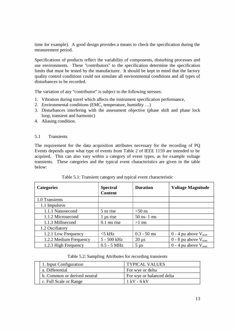
5.1 Transients

The requirement for the data acquisition attributes necessary for the recording of PQ Events depends upon what type of events from Table 2 of IEEE 1159 are intended to be acquired. This can also vary within a category of event types, as for example voltage transients. These categories and the typical event characteristics are given in the table below:

Table 5.1: Transient category and typical event characteristic

Categories Spectral Content

Duration Voltage Magnitude

1.0 Transients 1.1 Impulsive 1.1.1 Nanosecond 5 ns rise <50 ns 1.1.2 Microsecond 1 µs rise 50 ns- 1 ms 1.1.3 Millisecond 0.1 ms rise >1 ms 1.2 Oscillatory 1.2.1 Low Frequency <5 kHz 0.3 - 50 ms 0 - 4 pu above Vnom 1.2.2 Medium Frequency 5 - 500 kHz 20 µs 0 - 8 pu above Vnom 1.2.3 High Frequency 0.5 - 5 MHz 5 µs 0 - 4 pu above Vnom

Table 5.2: Sampling Attributes for recording transients

1. Input Configuration TYPICAL VALUES a. Differential For wye or delta b. Common or derived neutral For wye or balanced delta c. Full Scale or Range 1 kV - 6 kV

14

2. Input Impedance a. Resistance to Ground 10 - 40 M Ω b. Capacitance to Ground 40 pF c. Resistance Channel-to-Channel >50 MΩ 3. Input Filter a. High-pass cut-off frequency 5 - 10 kHz 4. Acquisition Scheme a. Low speed sampling 128 samples/channel/cycle b. Multi-sample/cycle peak detection 128 samples/channel/cycle c. High speed sampling 1 - Msamples/channel 5. Front End less the ADC a. Bandwidth 1 - 10 MHz b. Slew rate 9 - 30 V/?s c. Settling time 250 ns - 2 ?s d. Linearity e. Accuracy 10% error overall f. Common-mode rejection >40 dB @ 60 Hz g. Over/undershoot 6. Phase Shift between Samples a. Sequential 0.2 - 0.7° @ 60 Hz b. Simultaneous Sample and Hold <0.1° @ 60 Hz 7. Analog-to-Digital Conversion a. Conversion Time 250 ns - 3 ?s b. Reset time 500 ns (peak detectors) c. Bits Resolution 12 (pk det.) 8 - 10 (high speed) d. Conversion Accuracy +/- 1LSB 8. Samples a. Number of pre-trigger samples 0 – 512 b. Number of post-trigger samples 0 - 512 c. Phase position accuracy (time

correlation) +/- 1 LF sample

9. Trigger a. Absolute Value (peak relative to zero

volts) n/a

b. Relative (remove low frequency signals) n/a

B. Performance Criteria

1. Amplitude accuracy versus duration and point-on-wave of transient, including positive and negative transients.

2. Point-on-wave accuracy versus magnitude and duration

15

3. Duration accuracy versus magnitude and point-on-wave

4. Amplitude and frequency accuracy of oscillatory or ringing frequency.

5. Cross-channel coupling.

C. Test Waveforms

1. Lightning : 1.2 u x 50 µs

2. Surge Withstand Capability : 2 MHz exponentially decaying

3. PF Correction Cap switching In/Out : 2 pu, ½ cycle ring.

4. ANSI/IEEE C62.41-1991

5.2 Short duration variations

The short-duration variations include voltage interruption, sag and swell that were classified into three categories upon the duration of the phenomena (see Table 5.3). The short-duration variation assessment requests the measurement of the rms voltage deviation from the reference voltage Uref and the duration while the voltage remains below or above a predefined level. The reference voltage Uref is the value used for determining the depth of sag and the height of swell. This reference voltage can be predefined or calculated from the unaffected voltage previous to the variation detection. Sampling attributes for short-duration variation are defined upon the approach used to assess the voltage deviation form the reference voltage.

Table 5.3: Short-duration variation category and typical event characteristic

Categories Typical duration Typical voltage magnitude

2.0 Short duration variations 2.1 instantaneous 2.1.1 Sag 0.5-30 cycles 0.1-0.9 pu 2.1.2 Swell 0.5-30 cycles 1.1-1.8 pu 2.2 Momentary 2.2.1 Interruption 0.5 cycles-3 s < 0.1 pu 2.2.2 Sag 30 cycles-3 s 0.1-0.9 pu 2.2.3 Swell 30 cycles-3 s 1.14-1.4 pu 2.3 Temporary 2.3.1 Interruption 3 s-1 min <0.1 pu 2.3.2 Sag 3 s-1 min 0.1-0.9 pu

5.2.1 Attribute for depth or height measurement

16

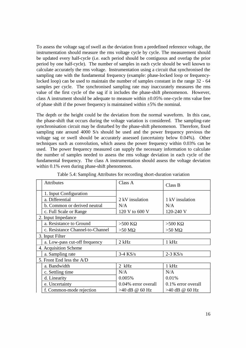
To assess the voltage sag of swell as the deviation from a predefined reference voltage, the instrumentation should measure the rms voltage cycle by cycle. The measurement should be updated every half-cycle (i.e. each period should be contiguous and overlap the prior period by one half-cycle). The number of samples in each cycle should be well known to calculate accurately the rms voltage. Instrumentation using a circuit that synchronised the sampling rate with the fundamental frequency (example: phase-locked loop or frequency-locked loop) can be used to maintain the number of samples constant in the range 32 - 64 samples per cycle. The synchronised sampling rate may inaccurately measures the rms value of the first cycle of the sag if it includes the phase-shift phenomenon. However, class A instrument should be adequate to measure within ±0.05% one-cycle rms value free of phase shift if the power frequency is maintained within ±5% the nominal.

The depth or the height could be the deviation from the normal waveform. In this case, the phase-shift that occurs during the voltage variation is considered. The sampling-rate synchronisation circuit may be disturbed by the phase-shift phenomenon. Therefore, fixed sampling rate around 4000 S/s should be used and the power frequency previous the voltage sag or swell should be accurately assessed (uncertainty below 0.04%). Other techniques such as convolution, which assess the power frequency within 0.03% can be used. The power frequency measured can supply the necessary information to calculate the number of samples needed to assess the rms voltage deviation in each cycle of the fundamental frequency. The class A instrumentation should assess the voltage deviation within 0.1% even during phase-shift phenomenon.

Table 5.4: Sampling Attributes for recording short-duration variation

Attributes Class A Class B

1. Input Configuration a. Differential 2 kV insulation 1 kV insulation b. Common or derived neutral N/A N/A c. Full Scale or Range 120 V to 600 V 120-240 V 2. Input Impedance a. Resistance to Ground >500 KΩ >500 KΩ c. Resistance Channel-to-Channel >50 MΩ >50 MΩ 3. Input Filter a. Low-pass cut-off frequency 2 kHz 1 kHz 4. Acquisition Scheme a. Sampling rate 3-4 KS/s 2-3 KS/s 5. Front End less the A/D a. Bandwidth 2 kHz 1 kHz c. Settling time N/A N/A d. Linearity 0.005% 0.01% e. Uncertainty 0.04% error overall 0.1% error overall f. Common-mode rejection >40 dB @ 60 Hz >40 dB @ 60 Hz

17

g. Over/undershoot

N/A N/A

6. Phase Shift between Samples a. Sequential 0.1 - 0.2° @ 60 Hz b. Simultaneous Sample and Hold <0.01° @ 60 Hz 7. Samples a. Number of cycles before

variations 2 cycles before the variation

b. Number of cycles after variations 2 cycle after the variation c. Phase position accuracy (time

correlation) +/- 1 LF samples

5.3 Long-duration variations

Long-duration variations yield to rms-voltage assessment. The accuracy of the rms voltage assessment during interruption is not obvious. Power interruption assumes the rms voltage level below a given level such as 10% of the reference voltage. To obtain comparable voltage assessment between instruments, the rms voltage should be measured over fixed window (e.g. 200-ms used for steady-state event). The sampling-rate synchronization circuit may not operate properly during very low-voltage level. Therefore, fixed sampling rate approach for assessing the voltage in each 200-ms window should be used.

The number of samples per cycle should be considered to assess the rms undervoltage and overvoltage values. Each window used to assess the rms voltage should correspond to exactly 12-cycles windows within 0.004 cycle. Since the power frequency may vary in time, the window-width accuracy may be provided by varying the number of samples per cycle or by varying the sampling rate according the power-frequency fluctuation. The accuracy of the power-frequency assessment or the sampling-rate synchronization circuit should be maintained for voltage level in the range 0.8-1.2 pu.

Table 5.5: Long-duration variation category and typical event characteristic

Categories Typical duration Typical voltage

magnitude 3.0 Long duration Variations 3.1 Interruption, sustained >1 min 0.0 pu 3.2 Undervoltages >1 min 0.8-0.9 pu 3.3 Overvotlages >1 min 1.1-1.2 pu

18

5.4 Voltage unbalance

Voltage- unbalance assessment is a steady-state event that calls for sampling each phase to ground or phase-to-phase fundamental voltage at a rate of at least 32 samples/cycle. A lower sampling rate can be used if an analog filter is used to remove the harmonic content from the signal. Three high-precision voltage transformers (<0.6%) are normally used to measure the voltage of MV or HV power systems. The voltage transformers used to assess voltage unbalance should be identical and loaded with identical impedances. Transformers feeding a 2-½ element metering system or an open-delta phase-to-neutral configuration should be avoided. The open delta voltage transformer connected phase-to-phase can be used if the load is identical on each transformer and if no load is connected on the open side of the open delta connection. The relative difference between the instrumentation input gains and phase could cause significant error in the assessment of power-system voltage unbalance. The accuracy of the absolute voltage-level assessment is not so important as long as each input to the instrument shows exactly the same error. If the instrument causes a relative 0.07% deviation between two input-voltage magnitudes and 0.05° deviation in the argument, the display can give up to 0.065% unbalance added or subtracted to the actual voltage unbalance level of the power system. For example, if such a 0.07% magnitude and 0.05° deviation occurs between two voltage input circuits of the instrument, the value displayed can range between 0.935% and 1.065% when 1.000% voltage unbalance appears on the power system. The input-gain fluctuation and the sequence of the sampling circuit can cause that deviation and add the error. Such good instrument input channel stability of less than 0.07% deviation in magnitude and 0.05° can also be affected during use and therefore the monitor should supply a tolerance test function. Therefore tolerance test before the unbalance voltage assessment can be performed. The tolerance test is the difference between the highest and the lowest input voltage magnitudes and the highest phase angle recorded when all probes are connected to the same voltage for 10 min. All harmonics should be filtered using an 8th-order filter or the DFT algorithm. Windows of 12 cycles for 60 Hz systems should be used for very rigorous assessment. The DFT results of such windows give spectral lines every 5 Hz. In this case, the fundamental is obtained at the 12th spectral line of the DFT output. The voltage amplitude on the power system may fluctuate, spreading out the energy of the fundamental to neighbourhood spectral lines. To improve the assessment accuracy of the voltage, the output components c for each 5 Hz neighbour of the fundamental frequency shall be grouped according to

2 2526 18

1 12 ii 5

c cC c

2 2+=−

= + +∑

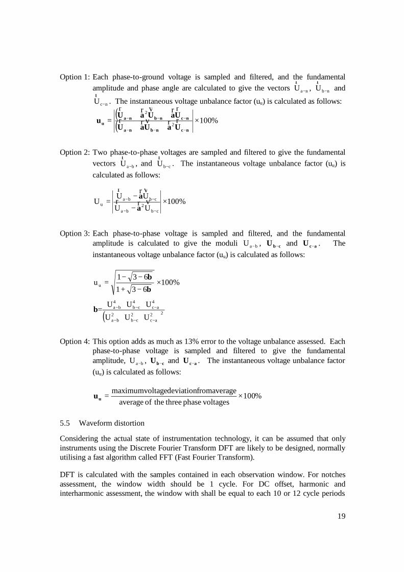
There are several options to calculate the voltage unbalance factor uu depending on the accuracy needed. Options 1 to 3 gives the most rigorous assessment but Option 4 adds a 13% error in the uu assessed.

19

Option 1: Each phase-to-ground voltage is sampled and filtered, and the fundamental amplitude and phase angle are calculated to give the vectors naU −

r, nbU −

r and

ncU −

r. The instantaneous voltage unbalance factor (uu) is calculated as follows:

( )( ) %100

2

2

×++++=

−−−

−−−

ncnbna

ncnbnau UaUaU

UaUaUu rrvrr

rrvrr

Option 2: Two phase-to-phase voltages are sampled and filtered to give the fundamental

vectors baU −

r, and cbU −

r. The instantaneous voltage unbalance factor (uu) is

calculated as follows:

cb

2ba

cbbau UU

UUU

−−

−−

−−= vrrvrr

aa ×100%

Option 3: Each phase-to-phase voltage is sampled and filtered, and the fundamental

amplitude is calculated to give the moduli baU − , cbU − and acU − . The instantaneous voltage unbalance factor (uu) is calculated as follows:

63+1

631u u β

β−−−= ×100%

( )22ac

2cb

2ba

4ac

4cb

4ba

UUU

UUU

−−−

−−−

++++=β

Option 4: This option adds as much as 13% error to the voltage unbalance assessed. Each

phase-to-phase voltage is sampled and filtered to give the fundamental amplitude, baU − , cbU − and acU − . The instantaneous voltage unbalance factor (uu) is calculated as follows:

%100 voltagesphase three theof average

averagefromdeviationvoltagemaximum ×=uu

5.5 Waveform distortion

Considering the actual state of instrumentation technology, it can be assumed that only instruments using the Discrete Fourier Transform DFT are likely to be designed, normally utilising a fast algorithm called FFT (Fast Fourier Transform).

DFT is calculated with the samples contained in each observation window. For notches assessment, the window width should be 1 cycle. For DC offset, harmonic and interharmonic assessment, the window with shall be equal to each 10 or 12 cycle periods

20

according the power-system frequency 50 Hz or 60 Hz. Therefore, the time between the leading edge of the first sampling pulse and the leading edge of the (M+1) th sampling pulse (where M is the number of samples in each window) should be equal to the duration of the specified number of cycles of the power system, with a maximum permissible error of ± 0,03%. For instruments requiring sampling-rate synchronisation means, the working input frequency range of the instrument should be at least ± 5% of the nominal system frequency. For noise assessment in the range 5-9 kHz, the window width should be 0.1 s.

The input circuit of the measuring instrument should be adapted to the nominal voltage and frequency of the supply voltage to be analysed and should keep its characteristics and accuracy unchanged up to 1,2 times this nominal voltage. A crest factor of at least 1,5 is considered sufficient for measurements except for highly distorting loads in industrial networks when a crest factor of a least 2 may be necessary. An overload indication is required in any case.

It is suggested that stressing the input for 1 s by an a.c. voltage of four times the input voltage setting or 1 kV r.m.s., whichever is less, should not lead to any damage in the instrument.

Many nominal supply voltages between 60 and 600 V exist, depending on local practice. To permit a relatively universal use of the instrument for most supply systems, it may be advisable for the input circuit to be designed for the following nominal voltages:

Un: 66, 115, 230 for 50 Hz systems

Un: 69, 120, 240, 277, 347, 480, 600 V for 60 Hz systems.

NOTES

1 The 66-, 69-, 115- and 120-V ranges may also be used in association with external voltage transformers. Other additional ranges may also be useful for that purpose (such as 100 V, 100/√3 V, 110/√3 V.

2 Inputs with higher sensitivity (0,1; 1; 10 V) are useful for operation with external transducers. A crest factor of at least 2 may be necessary.

Care should be taken that the high value of the fundamental (supply frequency) as compared to the harmonics to be measured does not produce overload causing damage or harmful intermodulation error signals in the input stages of the instrument. Such errors shall be well below the stated accuracy. Therefore an overload indication shall be provided.

The maximum allowable errors in Table 5.6 refer to single-frequency and steady-state signals, in the operating frequency range, applied to the instrument under rated operating conditions to be indicated by the manufacturer (temperature range, humidity range, instrument supply voltage, etc.).

21

Table 5.6: Sampling Attributes for recording short-duration variation Inom: Nominal current range of the measurement instrument

Vnom: Nominal voltage range of the measurement instrument Vm Im : Measured value

Class Measurement Conditions Maximum Error

A Voltage Vm ≥ 1% Vnom

Vm < 1% Vnom

5% Vm

0,05% Vm

Current

Im ≥ 3% I nom

Im < 3% I nom

± 5% I m

±0,15% Inom

B Voltage Um ≥ 3% Vnom

Um < 3% Vnom

5% Vm

0,15% Vm

Current

Im ≥ 10 % Inom

Im < 10 % Inom

± 5% I m

± 0,5% I nom

The frequencies outside the measuring range of the instrument (normally 0 to 6 kHz for harmonic and interharmonic and 40 kHz for notches and noise) should be attenuated so as not to affect the results. To obtain the appropriate attenuation, the instrument may calculate the frequency components at frequencies much higher than the measuring range. For example, the analysed range may reach 25 kHz, but only components up to 2 kHz are taken into account. An anti-aliasing low-pass filter, with a –3 dB frequency above the measuring range (such as 5 kHz) should be provided. The attenuation in the stop-band shall exceed 50 dB.

The achievement of the accuracy stated in Table 5.6 may require, according to clear indications to be given by the manufacturer, some simple adjustment of the instrument by means of an internal or external calibrator.

Table 5.7: Waveform distortion category and typical event characteristic

Categories Typical spectral content

Typical duration Typical voltage

magnitude 5.0 Waveform distortion Steady state 5.1 DC offset Steady state 0-0.1% 5.2 Harmonics DC-100 th H Steady state 0-20% 5.3 Interharmonics 0-6 kHz Steady state 0-2% 5.4 Notching 35 kHz Steady state 5.5 Noise Broad-band Steady state 0-1%

22

5.6 Voltage fluctuations

The voltage fluctuation is also called flicker. The observed phenomenon is the modulation of a carrier. In most cases the carrier is the fundamental frequency but harmonic frequency below 1 kHz can also provide the carrier.

Since the carrier needs to be processed, voltage input bandwidth should exceed 800 Hz to assess the voltage fluctuation. The frequencies outside the measuring range of the instrument (normally 1 kHz) should be attenuated so as not to affect the results.

The flickermeter defined in the IEEE 1453 includes analogue and digital circuits. Modern flickermeter circuit has reduced the analogue portion of the meter so as analogue circuit is limited to the voltage level interface. The voltage is then directly sampled after the antialiazing filter. The resolution of the sampling device is function of the sampling frequency. For example, some meters show very good performances with a 12-bits A/D converter at a sampling rate above 3 kS/s.

5.7 Power Frequency variations

The frequency of the power system is established by the angular velocity of mechanically connected prime movers and associated electrical generators. In large, networked power grids, the combined inertias of many large rotating generators operating synchronously provide an extremely stable system operating frequency. Power system deviations from nominal frequency rarely occur on large networks in developed countries. When significant deviations do occur, they usually result from slow clearance of severe faults, or cascading system failures that result in severe mismatches between available generation and connected loads. In less developed countries, there can be long term mismatches between available generation and connected loads that result in steady state under-frequency operation.

In small, isolated power systems, frequency deviations are more likely to occur when changes in connected loads are an appreciable fraction of the available generator kVA. Examples of this situation occur when isolated industrial loads are served from on-site generation and when commercial loads are served from on-site back-up generators. Remote communities served by local generators without a connection to a larger networked power grid may also experience frequency deviations due to switching on and off of “large” loads.

The results of frequency deviations on connected loads vary by type of load. As per IEEE Standard 446-1995, the majority of end-use equipment can tolerate frequency changes by as much as +/-0.5 Hz, which is slightly less than a one percent deviation on a 60 Hz system. Frequency deviations can affect the performance of electronic timers, where a timing interval is determined by detecting the zero-crossings of the ac supply voltage. Frequency deviations can also affect measurements of voltages where (frequency dependent) reactive components are involved.

23

Typically, power frequency variations on modern, interconnected power systems are rare. When they do occur on large systems, however, there exists the possibility for severe consequences such as sustained interruption of power. In such a scenario, frequency measurements are of interest in characterizing the dynamics of the power system during stressful conditions.

5.7.1 Measurement Techniques.

A variety of means are available for the measurement of synchronous power frequency. These include, and are not necessarily limited to, the following.

• Measured time interval between zero crossings of an ac input signal.

• Measured output frequency of a phase-locked-loop operating on an ac input signal.

• Use of a frequency-to-voltage converter, with an input derived from either the ac input signal or from a phase-locked-loop.

• DFT analysis of digitally sampled ac input waveform.

Rapid progress in electronic measurement technology of ac waveforms has opened the way for a variety of measurement application techniques. This standards document does not provide a specific recommended approach to ac frequency measurements, rather it outlines a test protocol for the “certification” of a meter’s ability to correctly measure ac input frequency under a variety of dynamic and steady-state conditions.

6. Performance test and calibration procedures

Several variation fields for parameters are considered. These are :

- reference conditions,

- specified operating range,

- limit of operating range,

- storage and transportation conditions.

The measurement of a specific voltage or current characteristic can be affected by the variation of another characteristic of the measured voltage or current. As a consequence, in this document, influence quantities include characteristics of the measured voltage or current in addition to "external" influence quantities.

6.1 Accuracy tests

The accuracy of the instrument should be tested for each sampling attribute as follows:

• Select a category to be tested (e.g. RMS voltage).

24

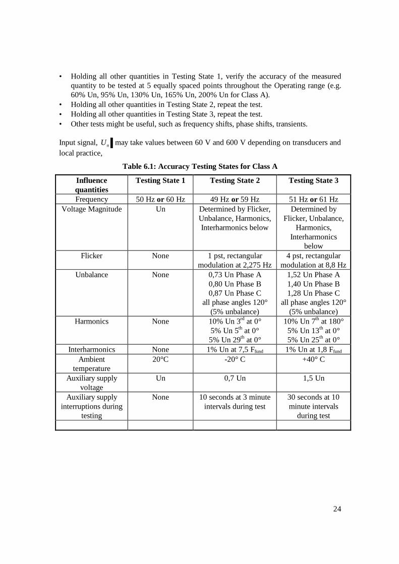
• Holding all other quantities in Testing State 1, verify the accuracy of the measured quantity to be tested at 5 equally spaced points throughout the Operating range (e.g. 60% Un, 95% Un, 130% Un, 165% Un, 200% Un for Class A).

• Holding all other quantities in Testing State 2, repeat the test. • Holding all other quantities in Testing State 3, repeat the test. • Other tests might be useful, such as frequency shifts, phase shifts, transients. Input signal, Un may take values between 60 V and 600 V depending on transducers and local practice,

Table 6.1: Accuracy Testing States for Class A

Influence quantities

Testing State 1 Testing State 2 Testing State 3

Frequency 50 Hz or 60 Hz 49 Hz or 59 Hz 51 Hz or 61 Hz Voltage Magnitude Un Determined by Flicker,

Unbalance, Harmonics, Interharmonics below

Determined by Flicker, Unbalance,

Harmonics, Interharmonics

below Flicker None 1 pst, rectangular

modulation at 2,275 Hz 4 pst, rectangular

modulation at 8,8 Hz Unbalance None 0,73 Un Phase A

0,80 Un Phase B 0,87 Un Phase C

all phase angles 120° (5% unbalance)

1,52 Un Phase A 1,40 Un Phase B 1,28 Un Phase C

all phase angles 120° (5% unbalance)

Harmonics None 10% Un 3rd at 0° 5% Un 5th at 0° 5% Un 29th at 0°

10% Un 7th at 180° 5% Un 13th at 0° 5% Un 25th at 0°

Interharmonics None 1% Un at 7,5 Ffund 1% Un at 1,8 Ffund Ambient

temperature 20°C -20° C +40° C

Auxiliary supply voltage

Un 0,7 Un 1,5 Un

Auxiliary supply interruptions during

testing

None 10 seconds at 3 minute intervals during test

30 seconds at 10 minute intervals

during test

25

Bibliography

Section 7:

Bibliography to be compiled and completed.