IEEE 802.11 Saturation Throughput Analysis in thePresence of Hidden Terminals

Beakcheol JangDept. of Computer Science

North Carolina State UniversityRaleigh, NC 27695

Email: bcjang@gmail.com

Mihail L. SichitiuDept. of Electrical and Computer Engineering

North Carolina State UniversityRaleigh, NC 27695

Email: mlsichit@ncsu.edu

Abstract—Due to its usefulness and wide deployment, IEEE802.11 has been the subject of numerous studies but still lacksa complete analytical model. Hidden terminals are common inIEEE 802.11 and cause the degradation of throughput. Despitethe importance of the hidden terminal problem, there have beena relatively small number of studies that consider the effect ofhidden terminals on IEEE 802.11 throughput, and many are notaccurate for a wide range of conditions. In this paper, we presentan accurate new analytical saturation throughput model for theinfrastructure case of IEEE 802.11 in the presence of hiddenterminals. Simulation results show that our model is accurate ina wide variety of cases.

I. I NTRODUCTION

IEEE 802.11 is one of the most widely adopted standardsfor Wireless Local Area Network since its development bythe IEEE LAN/MAC Standards Committee in 1996. Manyamendments have been standardized and widely deployed ina number of devices such as personal computers, laptops,mobile phones, home networks and other electronic devicesthat benefit from wireless networking due to their advantagessuch as low cost, high throughput and convenience. Thestandard has three MAC algorithms: CSMA/CA, RTS/CTSand PCF. This study is limited to the widely implementedCSMA/CA and RTS/CTS.

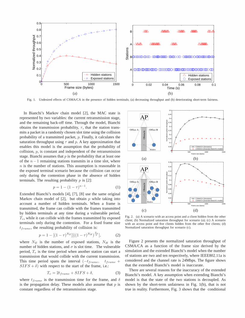
Hidden terminals are common in IEEE 802.11 because thecommunication and carrier-sense ranges of the access pointand clients vary significantly due to obstacles, interference,transmission power, antenna gain, and location. Despite worktoward alleviating the effects of hidden terminals, eitherbydeployment or node design [12], in real deployments withthe standard protocol, there will be hidden terminal situations.Hidden terminals effectively disable the carrier sense capabil-ity of the protocol and negatively affect the performance ofsystem. Figure 1 presents simulation results for CSMA/CA ofIEEE 802.11a at the data rate of 12Mbps: normalized satu-ration throughput and sequence traces of frames successfullyreceived by the access point for two scenarios with an access

point and two stations that are either exposed1 or hidden fromeach other. In the scenarios, stations are in the communicationrange of an access point and always have packets to sendto the access point. Figure 1 (a) shows that the saturationthroughput severely deteriorates in the hidden station scenarioas the frame size increases. Because the collision probabilityincreases with the frame size in the hidden station scenario, theresulting saturation throughput decreases. Figure 1 (b) showsthat the hidden terminal scenario is not fair on the short-termtime scale. This short-term unfairness negatively affectsupperlayer protocols such as TCP timeouts and high jitter for real-time audio and video streams [16].

In this paper, we present a new analytical saturation through-put model for CSMA/CA and RTS/CTS of IEEE 802.11 forcommon infrastructure scenarios with hidden stations. Wethen evaluate the accuracy of the model through extensivesimulations. The simulation result shows that our model isvery accurate for a wide range of conditions.

II. PROBLEM DEFINITION AND RELATED WORK

In this section, we define the problem tackled in this paperand briefly summarize the related work.

A. Problem Definition

Bianchi [2] presents a novel Markov chain model for thesaturation throughput for IEEE 802.11 in the absence ofhidden terminals. This study has been considered as one ofthe seminal papers for the throughput model of IEEE 802.11,and has been extended in many subsequent studies [2]–[5],[7], [8], [14]–[16], [19], [20], [24], [25]. A few of them, [4],[7], [8] extend Bianchi’s model to consider hidden terminals.In this paper, we call the similar models in [4], [7], [8]extended Bianchi’s models (although other papers extendedBianchi’s model in other directions, we are only interestedinhidden terminal extensions). However, Bianchi’s model cannotaccurately model hidden terminals as we will shortly explain.

1Traditionally, “exposed nodes” refer to nodes in a situation where theyare prevented from transmitting simultaneously due to carrier sense, althoughtheir simultaneous transmissions would be successful [13]. In this paper wedo not consider such topologies, and we refer to nodes that can sense thecarrier of each other as exposed nodes.

0 500 1000 15000

0.1

0.2

0.3

0.4

0.5

0.6

0.7

0.8

0.9

Frame size (bytes)

Nor

mal

ized

thro

ughp

ut

Hidden stationsExposed stations

0 0.02 0.04 0.06 0.08 0.1

A

B

A

B

Time (s)

Sta

tions

Hidden stationsExposed stations

(a) (b)

Fig. 1. Undesired effects of CSMA/CA in the presence of hidden terminals; (a) decreasing throughput and (b) deteriorating short-term fairness.

In Bianchi’s Markov chain model [2], the MAC state isrepresented by two variables: the current retransmission stage,and the remaining back-off time. Through the model, Bianchiobtains the transmission probability,τ , that the station trans-mits a packet in a randomly chosen slot time using the collisionprobability of a transmitted packet,p. Finally, it calculates thesaturation throughput usingτ andp. A key approximation thatenables this model is the assumption that the probability ofcollision, p, is constant and independent of the retransmissionstage. Bianchi assumes thatp is the probability that at least oneof then−1 remaining stations transmits in a time slot, wheren is the number of stations. This assumption is reasonable inthe exposed terminal scenario because the collision can occuronly during the contention phase in the absence of hiddenterminals. The resulting probabilityp is [2]:

p = 1 − (1 − τ)n−1. (1)

Extended Bianchi’s models [4], [7], [8] use the same originalMarkov chain model of [2], but obtainp while taking intoaccount a number of hidden terminals. When a frame istransmitted, the frame can collide with the frames transmittedby hidden terminals at any time during a vulnerable period,Tv, while it can collide with the frames transmitted by exposedterminals only during the contention. For a fixed frame sizetframe, the resulting probability of collision is:

p = 1 − [(1 − τ)NE ][((1 − τ)NH )Tvσ ], (2)

where NE is the number of exposed stations,NH is thenumber of hidden stations, andσ is slot time. The vulnerableperiod,Tv is the time period when another station can start atransmission that would collide with the current transmission.This time period spans the interval(−tframe, tframe +SIFS + δ) with respect to the start of the frame, i.e.:

Tv = 2tframe + SIFS + δ, (3)

where tframe is the transmission time for the frame, andδ

is the propagation delay. These models also assume thatp isconstant regardless of the retransmission stage.

0 500 1000 15000

0.05

0.1

0.15

0.2

0.25

0.3

0.35

0.4

0.45

0.5

Frame size (bytes)

Nor

mal

ized

sys

tem

thro

ughp

ut

CSMA/CA (Simulation)CSMA/CA (Extended Bianchi’s model)

(a) (b)

0 500 1000 15000

0.02

0.04

0.06

0.08

0.1

0.12

0.14

0.16

0.18

Frame size (bytes)

Nor

mal

ized

sys

tem

thro

ughp

ut

CSMA/CA (Simulation)CSMA/CA (Extended Bianchi’s model)

(c) (d)

Fig. 2. (a) A scenario with an access point and a client hiddenfrom the otherclient; (b) Normalized saturation throughput for scenario (a); (c) A scenariowith an access point and five clients hidden from the other fiveclients; (d)Normalized saturation throughput for scenario (c).

Figure 2 presents the normalized saturation throughput ofCSMA/CA as a function of the frame size derived by thesimulation and the extended Bianchi’s model when the numberof stations are two and ten respectively, where IEEE802.11aisconsidered and the channel rate is 24Mbps. The figure showsthat the extended Bianchi’s model is inaccurate.

There are several reasons for the inaccuracy of the extendedBianchi’s model. A key assumption when extending Bianchi’smodel is that the state of the two stations is decoupled. Asshown by the short-term unfairness in Fig. 1(b), that is nottrue in reality. Furthermore, Fig. 3 shows that the conditional

0 1 2 3 4 5 60.1

0.2

0.3

0.4

0.5

0.6

0.7

0.8

0.9

1

Retransmission stage

Col

lisio

n pr

obab

ility

2 hidden station scenario10 hidden station scenario

Fig. 3. Conditional collision probability as a function of retransmissionstage for the scenario in Fig. 2 (a) and Fig. 2 (c) when the framesize is 250bytes.

collision probability is not constant but rather increaseswiththe retransmission stage in scenarios of Fig. 2. The variationof the conditional collision probability is especially severewhen the number of stations is small.

In this paper, we present an accurate new Markov chainmodel reflecting the variation of the conditional collisionprobability as a function of the retransmission stage for thesaturation throughput for IEEE 802.11 in the presence ofhidden terminals for the general infrastructure cases. Thenew model takes into account the interactions between thetwo stations by jointly modeling the backoff stage of each ofthe two stations.

B. Related Work

Work in [4], [8], [20], [25] provides throughput models forIEEE 802.11 in the presence of hidden terminals. Work in[4] consider the infrastructure case, while [8], [20], [25]focuson the ad-hoc case. Ekici et al. [4] extend Malone’s model[19] to analyze IEEE 802.11 throughput without saturationfor the infrastructure case with hidden nodes. This modelassumes that the collision probability is constant regardlessof the retransmission stage. Although the simulation resultshows that the model is accurate in a scenario with two hiddenstations, the model is accurate only when the offered load issmall. As the load increases, the results of the model becomeinaccurate as shown in Fig. 2.

Work in [8], [20], [25] presents analytical models for multi-hop and ad-hoc networks. Hou et al. [8] analyze the throughputof the IEEE802.11 DCF scheme using the RTS/CTS accessmechanism in multi-hop ad-hoc networks. The simulationresults show that the model is accurate; however, if this modelis applied to CSMA/CA, it becomes inaccurate, as it does notconsider the retransmission stage for obtaining the collisionprobability. Work in [25] presents an analytical model forderiving saturation throughput in multi-hop ad hoc networkswith nodes randomly placed according to a two dimensionalPoisson distribution. In [20] the authors show that in saturated

multihop networks hidden terminals result in high packet-lossrate, routing instability and unfairness problems. The authorsshows that controlling the offered load at the sources caneliminate these problems. They also provide an analysis toestimate the optimal offered load that maximize the throughputof a multi-hop traffic flow. The paper provides both simulationresults and experimental results with a real six-node multi-hopnetwork.

The authors of [6] consider the twelve distinct cases of twocontending flows, showing that the hidden terminal problem isequivalent to one of the symmetric cases with incomplete state(SIS). The authors also show that in this case severe short-term(on the order of seconds) unfairness may occur. The authorsuse an generalized Bianchi model to capture the behavior insome of those cases.

In [17] the authors clearly point to the causes of short-termunfairness in scenarios with hidden terminals, and, further-more,quantify the unfairness by using a Markov chain modelfor the state of the system. The authors use a three variablestate for the Markov chain with the retransmission stages ofthe two hidden stations as two of the variables and the stateof the medium (e.g., idle, collision) as the third variable.Theycarefully compute the transition probabilities from each ofthese states and use them to quantify the short term unfairnesspresent in these hidden terminal situations.

In [22] the authors extend the results of [2] by incorpo-rating different transition probabilities in the two-dimensionalMarkov chain from [2] as a function of not only retransmissionstage. The model in [22] employs the same states as the modelin [2] (i.e., backoff state of a station), but the authors updatethe transition probabilities as a function of the positionsof theinterfering nodes with respect to the transmitting nodes (15different cases in all) and taking into account the probabilitiesof occurrence of each of the cases. In contrast, the modelproposed in this paper uses the retransmission stage of eachstation as system state. The authors further develop the modelin [21] by noting the drawbacks of using Bianchi’s model fora hidden terminal situation, specifically the ambiguity of avariable-time slot when stations have incomplete knowledgeof the channel state and solve it by adopting a fixed-size slotthat is modeled by introducing additional states in Bianchi’soriginal model.

A similar approach employing fixed time slots and addi-tional states in the Markov chain was used in [26]. In the samevein [9] use a discrete time slot for a relatively simple, buteffective model employing a Markov chain that only modelsthe state of the medium with four states (with nodes in regionA active or not and nodes in region B active or not).

In [27] the authors developed an analytical model for thepacket loss, delay and delay jitter for unsaturated networksand validated the model against simulations for low offeredloads.

The work in [23] focuses on IEEE 802.11 networks withbase stations and multiple terminals hidden from each otherin a saturated environment. The state of proposed modelis represented by the number of stations active, and the

AP

Obs

tacl

e

Hidden

A B

ExposedExposed

(a)

AP

D

B

A

C

E(4-to-1)

(4-to-1)

(4-to-1)(3-to-2)

(3-to-2)

(b)

Fig. 4. Hidden terminal scenarios; (a) Example ofna-to-nb infrastructurescenario with hidden terminals, where there are six exposed stations in regionA and four exposed stations in region B. Stations in different regions arehidden from each other. and (b) Example of general infrastructure scenario,where there are5 stations in the communication range of the access point,and the stations may irregularly be exposed or hidden from each other.

authors carefully compute the probabilities that each stationcan switch state from active to inactive. For computing thetransition probabilities the authors consider each possible caseof collision (destructive or not), success or idle slots, andcompute the probability of occurrence of each of these events.In contrast, we initially focus on the (simpler) case with onlytwo hidden station and use the retransmission stage of eachstation as system state.

III. A NALYTICAL MODEL

In this section, we present saturation throughput modelsusing a Markov chain model for IEEE 802.11 DCF for generalinfrastructure scenarios in the presence of hidden terminalspresented in Fig. 4. We assume that stations always haveframes to transmit to the access point, as we are interestedin the saturation throughput. We assume that the payload sizeis fixed. The access point does not transmit any data frameand only receives the frames from the stations and transmitsACKs to the stations. In Sec. III-A and III-B, we present asaturation throughput model for the infrastructure scenario inFig. 4 (a) in case that bothna andnb are one. In Sec. III-C, weextend the model presented in Sec. III-B for the infrastructurescenario havingmanystations neatly separated into two groupsas shown in Fig. 4 (a). Since the access point acts like aregular station when transmitting, this case also handles thecase when the AP is transmitting data to the clients. Finally, inSec. III-D, we model the saturation throughput of thegeneral

infrastructure scenarios with a mixture of hidden and exposedstations in Fig. 4 (b) using the model of Sec. III-C.

A. Simple Model for the IEEE 802.11 Network with TwoHidden Terminals

In this simple model, we consider two hidden terminalscenario, in which there are an access point and two stations,A andB. The stations are exposed to the access point but theyare hidden from each other. As a simplification, in this sectionwe ignore the fact that the result of previous transmissionscanaffect the next transmissions in IEEE 802.11 to simplify theproblem. Specifically, we make two simplifying assumptionsthat will be removed in Sec. III-B:

• we assume that when a successful transmission occurs,all stations choose new random back-off times instead ofhalting and restarting the previous back-off time in thenext transmission attempt;

• we assume that when a collision occurs, all stations starttheir next transmission attempts at the same time, i.e.,after the station that later transmits the lost frame endsits ACK timeout.

1) System State Model:Our system model is based on atwo dimensional Markov chain as shown in Fig. 5. Although atthe first glance this may look similar to Bianchi’s model [2],the two are fundamentally different: while Bianchi’s modelrepresents the state of anode, with retransmission stage andback-off counters defining the state, our model represents thestate of the entiresystem, by using the retransmission stageof each station as system state. The system changes statewhen the stations change their retransmission stage, as a resultof either a successful transmission or a collision, i.e., afterreceiving an acknowledgment, or after an acknowledgmenttimeout.

In this section, we define and then compute the systemstate probability matrixX. The elements of the probabilitymatrix X, xij represent the probability that stationA is in theretransmission stagei and stationB is in the retransmissionstagej for i, j ∈ {0,m − 1}, where m is the maximumretransmission limit. The retransmission stages,i and j, startfrom 0 at the first transmission and are increased by one everytime a transmission results in a collision, up tom − 1. Weconstruct the Markov chain model of the system state by usingsystem states and transition probabilities between the states.By imposing the normalization condition to the system statemodel, we find the stationary system state probabilityX.

Whenever a transmission occurs, the system can move fromstate(i, j) to one of the following three states:

(i, j) →

(0, j), i, j ∈ {0,m − 1},

(i, 0), i, j ∈ {0,m − 1},

(i′, j′), i′ = (i + 1) mod m,

j′ = (j + 1) mod m.

(4)

The first and second transitions represent the cases whensuccessful transmissions occur. The first transition representsthe case when stationA transmits a frame successfully. Once a

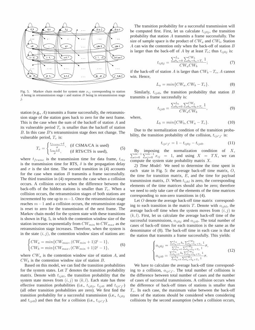
Fig. 5. Markov chain model for system statexij corresponding to stationA being in retransmission stagei and stationB being in retransmission stagej.

station (e.g.,A) transmits a frame successfully, the retransmis-sion stage of the station goes back to zero for the next frame.This is the case when the sum of the backoff of stationA andits vulnerable periodTv is smaller than the backoff of stationB. In this caseB’s retransmission stage does not change. Thevulnerable period,Tv is:

Tv =

{

tframe+δ

σ, (if CSMA/CA is used)

trts+δσ

, (if RTS/CTS is used),(5)

where tframe is the transmission time for data frame,trts

is the transmission time for RTS,δ is the propagation delayand σ is the slot time. The second transition in (4) accountsfor the case when stationB transmits a frame successfully.The third transition in (4) represents the case when a collisionoccurs. A collision occurs when the difference between theback-offs of the hidden stations is smaller thanTv. When acollision occurs, the retransmission stages of both stations areincremented by one up tom−1. Once the retransmission stagereachesm−1 and a collision occurs, the retransmission stageis reset to zero for the transmission of the next frame. TheMarkov chain model for the system state with these transitionsis shown in Fig. 5, in which the contention window size of thestation increases exponentially fromCWmin to CWmax as theretransmission stage increases. Therefore, when the system isin the state(i, j), the contention window sizes of stations are:

{

CWa = min{CWmax, (CWmin + 1)2i − 1},

CWb = min{CWmax, (CWmin + 1)2j − 1},(6)

whereCWa is the contention window size of stationA, andCWb is the contention window size of stationB.

Based on this model, we can find the transition probabilitiesfor the system states. LetT denotes the transition probabilitymatrix. Denote withtijkl, the transition probability that thesystem state moves from(i, j) to (k, l). Each state has threeeffective transition probabilities (i.e.,tij0j , tiji0 and tiji′j′ )(all other transition probabilities are zero). We first find thetransition probability for a successful transmission (i.e., tij0j

and tiji0) and then that for a collision (i.e.,tiji′j′ ).

The transition probability for a successful transmission willbe computed first. First, let us calculatetij0j , the transitionprobability that stationA transmits a frame successfully. Thesize of sample space is the product ofCWa andCWb. StationA can win the contention only when the back-off of stationB

is larger than the back-off ofA by at leastTv; thus tij0j is:

tij0j =

∑La

ba=0

∑CWb

bb=ba+Tv1

CWaCWb

; (7)

if the back-off of stationA is larger thanCWb−Tv, A cannotwin. Hence,

La = min{CWa, CWb − Tv}. (8)

Similarly, tiji0, the transition probability that stationBtransmits a frame successfully is:

tiji0 =

∑Lb

bb=0

∑CWa

ba=bb+Tv1

CWaCWb

, (9)

where,Lb = min{CWb, CWa − Tv}. (10)

Due to the normalization condition of the transition proba-bility, the transition probability of the collision,tiji′j′ is:

tiji′j′ = 1 − tij0j − tiji0. (11)

By imposing the normalization condition ofX,∑m−1

i=0

∑m−1j=0 xij = 1, and using X = TX, we can

compute the system state probability matrixX.2) Time Model: We need to determine the time spent in

each state in Fig. 5: the average back-off time matrix,O,the time for transition matrix,E, and the time for payloadtransmission matrix,D. Whentijkl is zero, the correspondingelements of the time matrices should also be zero; thereforewe need to only take care of the elements of the time matricescorresponding to non-zero transitions in (4).

Let O denote the average back-off time matrix correspond-ing to each transition in the matrixT . Denote withoijkl, theaverage back-off time when the system moves from(i, j) to(k, l). First, let us calculate the average back-off time of thesuccessful transmissions,oij0j andoiji0. The total number ofcases of back-off times for each transition is the same as thedenominator of (8). The back-off time in each case is that ofthe station that transmits a frame successfully. This yields:

oij0j =

PLaba=0

ba

PCWbbb=ba+Tv

1PLa

ba=0

PCWbbb=ba+Tv

1σ,

oiji0 =

PLbbb=0

bb

PCWaba=bb+Tv

1PLb

bb=0

PCWaba=bb+Tv

1σ.

(12)

We have to calculate the average back-off time correspond-ing to a collision,oiji′j′ . The total number of collisions isthe difference between total number of cases and the numberof cases of successful transmissions. A collision occurs whenthe difference of back-off times of stations is smaller thanTv. In each case, the maximum value between the back-offtimes of the stations should be considered when consideringcollisions by the second assumption (when a collision occurs,

RTSDIFS timeout

Time for successful transmission for CSMA/CA ( i.e., eij0j , eiji0 )

backoff

Time for successful transmission for RTS/CTS ( i.e., eij0j, eiji0 )

Time for collision for CSMA/CA ( i.e., eiji’j’ )

Time for collision for RTS/CTS ( i.e., eiji’j’ )

DIFS backoff Data SIFS ACK

DIFS backoff Data timeout

DIFS backoff RTS SIFS CTS SIFS Data SIFS ACK

Fig. 6. Time spent in state(i, j) given that the system transitions in state(k, l) (either successful transmission or collision)

all stations start their next transmission attempts at the sametime right after the station transmitting the lost frame laterends its timeout for ACK.) Thus:

oiji′j′ =

(PCWa

ba=0

Pba+Tv−1

bb=babb +

PCWbbb=0

Pbb+Tv−1

ba=bbba)σ

CWaCWb −PLa

ba=0

PCWa

bb=ba+Tv1−

PLbbb=0

PCWbba=bb+Tv

1.

(13)

Let E denote the time matrix representing time spent ineach transition in the matrixT . Denote witheijkl the timethe system spends in state(i, j) given that it will transitionin state(k, l). The time spent in state(i, j) for a successfultransmissions,eij0j is as shown in Fig. 6:

eij0j =

DIFS + oij0j + tframe + SIFS + δ + tack + δ,

(if CSMA/CA is used)

DIFS + oij0j + trts + SIFS + δ + tcts + SIFS

+δ + tframe + SIFS + δ + tack + δ,

(if RTS/CTS is used)(14)

where tframe, tack, trts and tcts are transmission times fora frame,ACK, RTS andCTS respectively. We obtaineiji0

by replacingoij0j with oiji0.When a collision occurs, the station waits for the timeout

instead of receiving the ACK or CTS. The time for a collision,eiji′j′ is as shown in Fig. 6:

eiji′j′ =

DIFS + oiji′j′ + tframe + δ + ttimeout,

(if CSMA/CA is used)

DIFS + oiji′j′ + trts + δ + ttimeout,

(if RTS/CTS is used)(15)

wherettimeout is the expected time for receiving ACK or CTSpacket. This yields:

ttimeout =

{

SIFS + tack + δ, (if CSMA/CA is used)

SIFS + tcts + δ. (if RTS/CTS is used)(16)

Let D denote the payload transmission time matrix. Denotewith dijkl, the time to send the payload when in state(i, j) andtransitioning in state(k, l). The payload is the data portion ofthe frame. When a collision occurs,diji′j′ is zero. The payloadtime for successful transmissions,dij0j , diji0, is the payloadtransmission time as it is. This yields:

dij0j = diji0 = tpayload. (17)

3) Saturation Throughput Model:Let S denote the nor-malized saturation system throughput, defined as the fractionof time the channel is used to successfully transmit payloadbits. X represents normalized time for each state andT isthe transition probability. The normalized saturation systemthroughput is equal to the total time spent in the payloadtransmission the payload transferred divided by the total timespent by the system. Thus:

S =

Pm−1

i=0

Pm−1

j=0

Pm−1

k=0

Pm−1

l=0xijdijklt

sijkl

Pm−1

i=0

Pm−1

j=0

Pm−1

k=0

Pm−1

l=0(xije

sijklt

sijkl + xije

cijklt

cijkl)

,

(18)wheretsijkl is the transition probability for a successful trans-mission,es

ijkl is the time spent in successful transmission,tcijkl

is the transition probability for a collision andtcijkl is the timespent in a collision.

B. An Enhanced Model for the IEEE 802.11 Network withTwo Hidden Terminals

This model enhances the simple model in Sec. III-A tobetter match the behavior of IEEE 802.11. The enhancedmodel operates under the same assumptions presented in Sec-tion III, but removes the two additional assumptions introducedin Section III-A. The enhanced model accounts for the fact thatin IEEE 802.11 the results of the previous transmission affectthose of the next transmission. Specifically:

• when a successful transmission occurs, the hidden stationthat did not transmit, overhears the ACK frame, it haltsits countdown and then resumes it with the remainingback-off time in the next transmission attempt. That is,the back-off time of the hidden station reduces as muchas sum ofTv and the winner’s back-off time after asuccessful transmission.

• when a collision occurs, the starting time instances of thenext transmission attempts of the stations that collided(when they are hidden from each other) are different.

1) System State Model:In developing the extended modelwe recognize that the system we model isnot a Markovsystem, as the transition probabilities from the current state tothe next state are also a function of the past states; however, theextended model we use is a Markov chain where the enhancedtransition probabilities will also take into account the paststates. We define an enhanced transition probability matrix,T ′. Denote witht′ijkl, the enhanced transition probability thatthe system state moves from(i, j) to (k, l). We assume thatstate (i, j) is the current state,(k, l) is the next state, and(p, q) is the previous state withi, j, k, l, p, q ∈ {0,m−1}. InT ′, the next transition probabilities (i.e.,t′ijkl) depend on the

Fig. 7. Example of a successful transmission occurring in the previoustransition.

result of previous transition. To obtaint′ijkl, we consider twothings. First, we consider the probability that the system state(i, j) occurred from a transition from the system state(p, q).We denote this probability withppqij . Thus:

ppqij =tpqijxpq

∑m−1p=0

∑m−1q=0 tpqijxpq

. (19)

Second, we consider the adjustment of the next transitionprobability by taking into account the previous transition(either a successful transmission or a collision). We denotethis adjustment witht”pqij

ijkl . These yield:

t′ijkl =m−1∑

p=0

m−1∑

q=0

ppqijt”pqijijkl . (20)

Thus we can obtain the transition probability for successfultransmissions (i.e.,t′ij0j and t′iji0). The transition probabilityfor collision, t′iji′j′ , is simply obtained by the normalizationcondition:

t′iji′j′ = 1 − t′ij0j − t′iji0. (21)

The adjustment in the transition probability,t”pqijijkl , depends

on whether the previous transition was a successful transitionor a collision. We first focus on how the next transition proba-bility (i.e., t”pqij

ijkl ) should be adjusted when the previous tran-sition was a successful transmission. Figure 7 shows the casewhen a successful transmission occurred during the previoustransition, where stationB transmitted a frame successfully.Station A performs the back-off countdown, overhears theACK frame and it halts its back-off countdown; it then resumesthe remaining back-off countdown in the next transmissionattempt; therefore the back-off time of the station that didnottransmit a frame (i.e.,A) reduces on average by sum ofTv

from (5) and the average back-off time of the station that didtransmit a frame (i.e.,B). This can be effectively modeledby considering that the back-off time of the station that didnot transmit the frame is chosen from a smaller contentionwindow:

t”pqijijkl =

tijkl(CWa, CWb − nrCWr),

(if A transmitted a frame successfully)

tijkl(CWa − nrCWr, CWb),

(if B transmitted a frame successfully)

(22)

where the expressiontijkl(a, b) represents the value oftijkl asin (7), (9) and (11) with the contention window size of stationA being a and that of stationB being b, nr is the averagenumber of times of the contention window size to be reducedandCWr is the size of the reduction of the contention windowafter each successful transmission by the other station.CWr

is determined, as shown in Fig. 7:

CWr =opqij

σ+ Tv, (23)

The number of reductions in the contention window israndom, depending on the value of the backoff chosen by thestation that does not transmit; on the average, the expectednumber of reductions in the contention window,nr is half thenumber of times the reduction in the contention window fits inthe contention window of the station that does not transmit:

nr =l + 1

2, (24)

wherel is:

l =

{

CWb

CWr, if A transmitted a frame successfully,

CWa

CWr.if B transmitted a frame successfully.

(25)

The transition probabilityt”pqijijkl in (22) captures the proba-

bility of a chain of transitions where one station successfullysends a series of one or more packets during the backoff ofthe other station. During all these transitions except possiblythe first one, the station sending packets is in backoff stagezero as it is successful in its transmission. For example, ifthe successful station isB while A is in backoff stageα, thetransitions modeled in (22) are(α, q) – (α, 0) – ... – (α, 0) –(k, l). On the average there arenr − 1 (α, 0) states betweenthe first and last state in the sequence. Strictly speaking, in thesequence of state transitions above, only during the first statetransition the value of the contention window ofA is decreasedby CWr given in (23), while for the other transitions, thevalue of CWr for q = 0 should be used. However, due tothe short term unfairness (illustrated in Fig. 1),q = 0 is thecommon case, and the approximation holds well. The previoustransition was a successful transmission if i6= ((p+1) mod m)or j 6= ((q+1) mod m). The retransmission stage of the stationthat transmits a frame successfully is reset to 0, thus i=0 meansthat A transmitted a frame successfully, while j=0 means thatB transmitted a frame successfully. Thus, if ((i6= ((p+1) modm)) or (j 6= ((q+1) mod m))) and if(i=0), thenA transmitteda frame successfully. Similarly, if((i6= ((p+1) mod m)) or (j6= ((q+1) mod m))) and if(j=0), thenB transmitted a framesuccessfully.

We now show how the next transition probability (i.e.,t”pqij

ijkl ) should be adjusted when the previous transition was a

Data

busy idle

Access Pointsystem state

Station B

Station A

12 11 10 9 8 7 6 5 4 3 2 1

DIFS back-off timeout DIFS back-off

DIFS timeout DIFS back-off

Data

1

idle

previous transmission next transmission

0 Tc Tv/2

Fig. 8. Example with a collision occurring in the previous transition.

collision. Figure 8 shows the case when a collision occurredinthe previous transition. The previous transition was a collisionif(i = ((p+1) mod m)) and (j = ((q+1) mod m)).

Let us consider the transition probability (i.e.,t”pqijij0j ) that

station A transmits a frame successfully in the next trans-mission attempt. First, let us consider the case when stationA transmitted a frame faster than stationB in the previoustransmission as shown in Fig. 8. If stationA chooses a back-offtime smaller thanTc (0 ≤ ba < Tc) in the next transmission,A cannot avoid a collision with the previous transmissionof station B. The average difference between the back-offtimes of two contending stations when a collision occurs isthe half of Tv because the collision occurs only when thedifference between the back-off times is smaller thanTv. Onthe other hand, because we assumed that station A transmittedthe frame faster than station B,Tc should not be a negativenumber; Tc is a random variable equal to the differencebetween the backoff of station B and the backoff of stationA during the previous transmission minus the number of timeslots taken by the timeout and DIFS. Under the assumptionof a collision in the previous state,Tc + ttimeout+DIFS

σcan

only take values between 0 andTv. Since Tc is uniformlydistributed, its average is:

T̄c = max{0,Tv

2−

ttimeout + DIFS

σ}. (26)

Therefore,0 ≤ ba < Tc should be excluded in the calculationof the successful transition probability.

If station A chooses a back-off time such thatTc ≤ ba ≤CWa, in order for stationA to transmit a frame successfully,stationB should choose a back-off time larger than stationA

by at least Tv; therefore the number of events when stationA transmits a frame successfully is:

EAA =

Tcmax∑

Tc=0

CWa∑

ba=Tc

CWb∑

bb=ba+Tv

1, (27)

whereTcmax= Tv − ttimeout+DIFS

σ.

Second, let us consider the case when stationB transmitteda frame faster than stationA in the previous transmission (andcollided) but A was successful in the next transmission. In thenext transmission stationB should choose a larger back-offtime than stationA by at least Tc + Tv in order for station

A to transmit a frame successfully because of the assumptionthat the back-off of stationB starts earlier than the back-offof stationA by Tc; therefore the number of events leading toa successful transmission by stationA is:

EAB =

Tcmax∑

Tc=0

CWa∑

ba=0

CWb∑

bb=ba+Tc+Tv

1. (28)

We assume that the probability thatA transmitted a framefaster thanB in the previous transmission is equal to the prob-ability that B transmitted faster thanA; therefore the samplespace of all the cases leading to a successful transmissionby A is 2Tcmax

CWaCWb. Thust”pqijij0j , the adjusted transition

probability that stationA transmits a frame successfully in thenext transition, is:

t”pqijij0j =

EAA + EAB

2TcmaxCWaCWb

, (29)

where i = ((p+1) mod m) and (j = ((q+1) mod m).In a similar way,t”pqij

iji0 , the adjusted transition probabilitythat stationB transmits a frame successfully in the nexttransition, is:

t”pqijiji0 =

EBA + EBB

2TcmaxCWaCWb

, (30)

whereEBA andEBB , are:{

EBA =∑Tcmax

Tc=0

∑CWb

bb=Tc

∑CWa

ba=bb+Tv1,

EBB =∑Tcmax

Tc=0

∑CWb

bb=0

∑CWa

ba=bb+Tc+Tv1.

(31)

We can calculatet′ij0j and t′iji0 using (20), (22), (29)and (30) andt′iji′j′ using (21). In result, we obtain theadjusted transition probability matrix,T ′, and by imposingthe normalization condition,

∑m−1i=0

∑m−1j=0 b′ij = 1, and using

X ′ = T ′X ′, we can obtain an enhanced stationary probabilitymatrix X ′.

2) Time Model:The time for transition matrix,E, and thetime for payload matrix,D, are similar to those of Sec. III-A(for matrix E the adjusted matrixO that is computed belowwill be used instead of the original one). The average back-off time matrix,O is also similar to that of Sec. III-A exceptthe average back-off time corresponding to a collision,oiji′j′ .In this model, we consider that the next transmission startsat the time when the station that transmitted a frame fasterin the previous transmission ends (e.g., station A in Fig. 8)the time-out for ACK in the previous transmission as in Fig.8; therefore the back-off time corresponding to a collisionisthe minimum back-off time of the two back-off times of thecontending stations. Thusoiji′j′ is:

oiji′j′ =

(PCWa

ba=0ba

Pba+Tv−1

bb=ba1 +

PCWbbb=0

bb

Pbb+Tv−1

ba=bb1)σ.

CWaCWb −PLa

ba=0

PCWbbb=ba+Tv

1−PLb

bb=0

PCWa

ba=bb+Tv1.

(32)

C. The Hidden Terminal Scenario with Two Groups of Stationsin Region A and Region B

In this section, we consider the infrastructure scenario withhidden stations shown in Fig. 4 (a).

While the exact dynamics of this scenario with multiplestation in each region are complex, we are able to approximatethese dynamics using a relatively simple enhancement of theone-to-one model in Sec. III-B.

The change accounts for the increase in the number ofstations in each region. As the number of stations in regionA increases (e.g., the number of stations in region A -na),it is more likely that a station in region A will win thecontention with the stations hidden in the region B, becausemore stations in region A will choose more random numbersas their contention window and the minimum of those numberswill be more likely to be sufficiently small to be successful.Because each station in region A is exposed to all otherstations in region A, the station that chooses the minimumvalue for its contention window will effectively prevent allother stations in its region from transmitting (as they willsense the carrier and back-off). Thus, we can model all stationsin region A as a single station with a modified contentionwindow. The contention window of the equivalent station isequal to the minimum of the contention window of allna

stations in region A. By considering the first term in theTaylor expansion for the minimum ofna identical stationwith uniformly distributed contention windows ofCWM , theequivalent station A’ will have a maximum contention windowCWM

na. Similarly, for region B, allnb stations in region B can

be modeled by a single equivalent station with a contentionwindow of CWM

nb:

CW ′

a = min{⌊

CWmax

na

⌋

, (⌊

CWmin

na

⌋

+ 1)2i − 1},

CW ′

b = min{⌊

CWmax

nb

⌋

, (⌊

CWmin

nb

⌋

+ 1)2j − 1},(33)

where⌊ ⌋ is the truncation function. The rest of the deriva-tion determining which station will succeed and with whatprobability do not change.

D. General Scenario

In this section, we consider the general infrastructurescenario with hidden stations shown in Fig. 4 (b). In thisscenario,n stations (e.g., 5 stations in Fig. 4 (b)) are randomlydistributed in the communication range of the access point,and they are arbitrarily exposed or hidden from each other.We model this general scenario by using the results of thena-to-nb scenario applied to each station. For example, stationA in Fig. 4 (b) has three exposed stations (na=3 includingitself) and two hidden stations (nb=2), such that we can saythat stationA is in the 3-to-2 scenario. Similarly, stationB isin a 4-to-1 scenario. Thus, we can model this general scenariofrom the perspective of each station using the results of thena-to-nb scenario.

The reasoning behind this extension is that, regardless ofthe exact topology of the network, each station will encounter

only two types of contending nodes: nodes that are exposed toitself and nodes that are hidden. As long as the models for thena-to-nb case estimates the correct state (backoff, throughput,etc.) state for each station, the aggregate throughput should bereasonably accurately predicted by this extension.

As we will show in the results section, this extension worksreasonably well even for relatively complex systems. Thereasons for the relative accuracy of this approximation arewell explained in [18]; in [18] the authors show that, as anapproximation (“back of the envelope”), the throughput of an802.11 node in a complex topology is primarily influencedby its direct neighbors and is largely independent of distantneighbors. From this perspective, the model in this sectionextends the simple model in [18] by taking into account thedirect neighbors and their hidden neighbors.

For example, the scenario in Fig. 4 (b) consists of twostations in 4-to-1 scenario (B and C) and three stations in 3-to-2 scenario (A, D and E). We can calculate the normalizedsaturation throughput of the general hidden terminal scenarioby calculating the weighted average of the normalized through-put of eachna-to-nb scenario using our model in Sec. III-C.Thus:

Sg =

∑lk=1 nkS(nak, nbk)

n, (34)

where Sg is the normalized saturation throughput of thegeneral infrastructure scenario with hidden stations,n is thenumber of stations in the scenario,l is the number of differentna-to-nb scenarios in the general scenario,nk is the numberof stations in thekth na-to-nb scenario, andS(nak, nbk)is the normalized saturation throughput of thekth na-to-nb scenario. For example, for the topology in Fig. 4 (b):Sg = 3S(4,1)+2S(3,2)

5 .

E. IEEE 802.11a Physical Layer Model

The 802.11a standard operates in 5 GHz band and usesOrthogonal Frequency-Division Multiplexing (OFDM) modu-lation. It provides eight payload data rates (i.e., 6, 9, 12,18,24, 36, 48, 54Mbps) with different modulation schemes (i.e.,BPSK, QPSK, 16-QAM and 64-QAM) and coding rates. Weshow how to obtain the transmission times of frame, payload,RTS, CTS and ACK for IEEE 802.11a. Refer to the IEEE802.11a standard [11] for a more complete presentation.

In IEEE 802.11a standard, the MAC data frame (i.e., MACProtocol Data Unit (MPDU)) consists of the MAC Header,payload (0 to 2312 bytes) and Frame Check Sequence (FCS).The MAC header and FCS together are 28 bytes, the RTSMPDU is 20 bytes, and the CTS and ACK MPDUs are14 bytes long. During transmission, a PLCP preamble anda PLCP header are added to the MAC frame to create thephysical layer frame (e.g., PLCP Protocol Data Unit (PPDU)).The PLCP preamble field, is composed of 10 repetitions ofa short training sequence (0.8µs) and two repetitions of along training sequence (4µs). The PLCP header except theSERVICE field constitutes a single OFDM symbol (4µs). The16-bit SERVICE field of the PLCP header and the MAC frame(along with six tail bits and pad bits) are transmitted at thedata

Parameters ValueMAC header size 34 bytesACK size 14 bytesRTS size 20 bytesCTS size 14 bytesCWmin 15CWmax 1023slot time 9 µsSIFS 16 µsDIFS 34 µs

TABLE ISIMULATION PARAMETERS FOR IEEE 802.11A .

rate specified in the RATE field. Therefore the transmissiontimes of data frame, RTS, CTS and ACK is;

tdata = tPLCPpreamble + tPLCPheader + tSERV ICEfield

+ttail + tMACheader + tFCS + tpayload,

= 16µs + 4µs + (16+6)+28∗8+payloadBit

dataRate(m) ,

trts = tPLCPpreamble + tPLCPheader + tSERV ICEfield

+ttail + trtsMPDU ,

= 16µs + 4µs + (16+6)+20∗8dataRate(m) ,

tcts = tPLCPpreamble + tPLCPheader + tSERV ICEfield

+ttail + tctsMPDU ,

= 16µs + 4µs + (16+6)+14∗8dataRate(m) ,

tack = tPLCPpreamble + tPLCPheader + tSERV ICEfield

+ttail + tackMPDU ,

= 16µs + 4µs + (16+6)+14∗8dataRate(m) .

(35)The frame formats of IEEE 802.11g [10] are the same as

those of IEEE 802.11a; therefore the transmission times ofdata frame, RTS, CTS and ACK of IEEE 802.11g are identicalto those of IEEE 802.11a.

IV. M ODEL VALIDATION

We compare the result of our model with that of extendedBianchi’s model and the result of detailed simulations.

A. Simulation Setup

We use the discrete event simulation environment, OM-NET++ [1], as the simulator and its mobility framework asthe simulation model for IEEE 802.11. The mobility frame-work considers the signal-to-noise ratio and the bit-errortodetermine whether a frame is transmitted correctly or not. Weconsider neither the signal-to-noise ratio nor bit-errorsin ourmodel and disable these features. Thus, the receiver considerscollisions the cases when it receives any other frames duringthe reception of a frame. OMNET++ mobility frameworkconsiders IEEE 802.11b. Because we are interested in IEEE802.11a, we modify the parameters of the physical layer ofIEEE 802.11 implementation of the mobility framework asshown in Sec. III-E. The parameters of IEEE 802.11a areshown in Table I.

We are interested in the saturation throughput; therefore theclients always have packets to send to the access point, and the

0 500 1000 15000

0.1

0.2

0.3

0.4

0.5

0.6

0.7

Frame size (bytes)

Nor

mal

ized

sys

tem

thro

ughp

ut

CSMA/CA (Simulation)CSMA/CA (Extended Bianchi’s model)CSMA/CA (Our enhanced model)CSMA/CA (Our simple model)

Fig. 9. Normalized saturation throughput for CSMA/CA as a function ofthe frame size at the payload data rate of 6Mbps.

access point does not transmit any data frame and only receivesthe data frames from the stations and replies with ACK frames.To obtain the normalized system throughput, we observe thenumber of frames per second received by the access point,Fn,and divide the product ofFn and the size of payload,Ps, bythe payload data rate,Dr. Therefore the normalized systemthroughputS (also known as channel utilization) is:

S =FnPs

Dr

. (36)

We consider frame size and payload data rate as evaluationparameters. In each simulation, the system runs for 300seconds.• Frame size: As frame size increases, the collision prob-

ability also increases, and in result, the throughput de-creases. In IEEE 802.11a, the maximum frame size atthe MAC level is 2346 bytes, but we consider the rangeof 0 to 1500 bytes, because the access point is almostalways connected to Ethernet in the infrastructure case,and the maximum frame size of Ethernet is 1500 bytes.

• Payload data rate: IEEE 802.11 provides eight payloaddata rates (6, 9, 12, 18, 24, 36, 48, and 54Mbps). Weconsider all of the data rates in our evaluations.

We consider three kinds of hidden terminal scenario; one-to-one,na-to-nb and general scenarios presented in Fig. 4.

B. Simulation Results and Analysis

In this section, we present simulation result and analysisfor one-to-one,na-to-nb and general hidden terminal scenariorespectively. We refer to the model developed in Sec III-Aas “our simple model”, to the extended model developed inSec. III-B as “our extended model”, and and to the one in [4],[7], [8] as ”Extended Bianchi’s Model”.

1) One-to-one scenario:Figures 9 to 11 show the normal-ized saturation throughput as a function of the frame size.For the CSMA/CA (Figs. 9 and 10), for small frames, as theframe size increases, the normalized throughput also increasesbecause the header induced overhead of the frame decreases.

0 500 1000 15000

0.1

0.2

0.3

0.4

0.5

0.6

0.7

Frame size (bytes)

Nor

mal

ized

sys

tem

thro

ughp

ut

CSMA/CA (Simulation)CSMA/CA (Extended Bianchi’s model)CSMA/CA (Our enhanced model)CSMA/CA (Our simple model)

Fig. 10. Normalized saturation throughput for CSMA/CA as a function ofthe frame size at the payload data rate of 54Mbps.

0 500 1000 15000

0.1

0.2

0.3

0.4

0.5

0.6

0.7

Frame size (bytes)

Nor

mal

ized

sys

tem

thro

ughp

ut

RTS/CTS (Simulation)RTS/CTS (Extended Bianchi’s model)RTS/CTS (Our enhanced model)

Fig. 11. Normalized saturation throughput for RTS/CTS as a function of theframe size at the payload data rate of 54Mbps.

After the normalized throughput reaches its maximum, itdecreases as the frame size increases because the vulnerableperiod that causes collisions also increases. Note that thevulnerable period increases with the frame size as shown in(3). The normalized throughput of CSMA/CA may appearhigh in comparison with a pure ALOHA system in Figs. 9and 10 (with a maximum value of about 0.35 to 0.4). Thisrelatively high channel utilization is due to the short-termunfairness problem caused by the binary exponential back-off used in IEEE 802.11, in which if a station transmits aframe successfully, the station resets its contention windowsize to the minimum. As a result, the winning station has asmaller back-off time than the other stations, and monopolizesthe channel (resulting in a decreased collision probability) untilanother station wins the contention. This effect deteriorates theshort-term fairness but increases the throughput. Our simplemodel (described in Section III-A) estimates the performanceof the system only in some situations, while showing asignificant inaccuracy in other situations. This performanceinconsistency of our simple model persists for a large range

0.5 1 1.5 2 2.5 3 3.5 4 4.5 5 5.5

x 107

0

0.1

0.2

0.3

0.4

0.5

0.6

0.7

Payload data rate (bps)

Nor

mal

ized

sys

tem

thro

ughp

ut

CSMA/CA (Simulation)CSMA/CA (Extended Bianchi’s model)CSMA/CA (Our enhanced model)

Fig. 12. Normalized saturation throughput for CSMA/CA as a function ofthe payload data rate at the frame size of 250 bytes.

0.5 1 1.5 2 2.5 3 3.5 4 4.5 5 5.5

x 107

0

0.1

0.2

0.3

0.4

0.5

0.6

0.7

Payload data rate (bps)

Nor

mal

ized

sys

tem

thro

ughp

ut

CSMA/CA (Simulation)CSMA/CA (Extended Bianchi’s model)CSMA/CA (Our enhanced model)

Fig. 13. Normalized saturation throughput for CSMA/CA as a function ofthe payload data rate at the frame size of 1500 bytes.

of parameters. To avoid cluttering the graphs, we will omitthe results of the simple model from the rest of the evaluationsection. Our extended model shows a good accuracy in Fig. 9and 10. The results of our extended model are very closeto those from the simulation, while the results of extendedBianchi’s model are relatively inaccurate. Due to the memory-less property of the Markov chain model, our model cannotexactly reflect the behavior of the real system; however, asshown in these figures, our enhanced model is very accurate.For RTS/CTS (Figs. 11), the throughput increases with theframe size because the size of the RTS frame is constantregardless of the frame size, resulting in a constant collisionprobability. For RTS/CTS, the results of extended Bianchi’smodel like those of our model match with those of thesimulation because the size of RTS frame is too small to affecton the collision probability.

Figures 12 to 14 present the normalized saturation through-put varying payload data rate. For CSMA/CA (Figs. 12 and13), the normalized throughput first increases with the dataratebecause the vulnerable period decreases with an increase in

0.5 1 1.5 2 2.5 3 3.5 4 4.5 5 5.5

x 107

0

0.1

0.2

0.3

0.4

0.5

0.6

0.7

0.8

0.9

Data rate (bps)

Nor

mal

ized

sys

tem

thro

ughp

ut

RTS/CTS (Simulation)RTS/CTS (Extended Bianchi’s model)RTS/CTS (Our enhanced model)

Fig. 14. Normalized saturation throughput for RTS/CTS as a function of thepayload data rate at the frame size of 1500 bytes.

1 2 3 4 5 6 7 8 9 100

0.1

0.2

0.3

0.4

0.5

0.6

0.7

0.8

Number of stations in region B

Nor

mal

ized

sys

tem

thro

ughp

ut

CSMA/CA (Simulation)CSMA/CA (Extended Bianchi’s model)CSMA/CA (Our enhanced model)

Fig. 15. Normalized saturation throughput forna=1 as a function ofnb forCSMA/CA, the number of stations in regionB, at the payload data rate of54Mbps and the frame size of 1500 bytes.

data rate. After it peaks, the normalized throughput decreasesbecause the physical layer header overhead of IEEE 802.11a isconstant regardless of the data rate resulting a reduced channelutilization. The results of our model are exactly same as thoseof the simulation. For RTS/CTS (Figs. 14), the throughputdecreases as the data rate increases because the physical layerheader overhead of IEEE 802.11a is constant regardless ofthe data rate. For RTS/CTS, both the results of extendedBianchi’s model and those of our model match with thoseof the simulation.

2) Thena-to-nb Scenario:Figure 15 shows the normalizedsaturation throughput for CSMA/CA as a function of thenumber of station for the hidden terminal scenario in Fig. 4 (a)fixing na=1 and varyingnb from one to ten. The normalizedthroughput is almost constant regardless ofnb, the number ofstations in the regionB. The increased number of exposedstations in the regionB increases the contention in regionB, but as the number of stations in the regionB increases,the frames from the station in regionA are more likely to

1 2 3 4 5 6 7 8 9 100

0.1

0.2

0.3

0.4

0.5

0.6

0.7

0.8

Number of stations in region A and B

Nor

mal

ized

sys

tem

thro

ughp

ut

CSMA/CA (Simulation)CSMA/CA (Extended Bianchi’s model)CSMA/CA (Our enhanced model)

Fig. 16. Normalized saturation throughput as a function ofna andnb forCSMA/CA, the number of stations in both regions, at the payload data rateof 54Mbps and the frame size of 1500 bytes.

0 500 1000 15000

0.1

0.2

0.3

0.4

0.5

0.6

0.7

0.8

0.9

1

Frame size (bytes)

Nor

mal

ized

sys

tem

thro

ughp

ut

CSMA/CA (Simulation)CSMA/CA (Extended Bianchi’s model)CSMA/CA (Our enhanced model)

Fig. 17. Normalized saturation throughput as a function of frame size forCSMA/CA for 4-to-1 scenario.

collide with frames from stations in regionB; as a result,the station in the regionA stays most of the time at a highretransmission stage. In the simulation, the number of framesthe station in the regionA transmits successfully decreasesas the number of stations in the regionB increases. On theother word, the number of frames stations in the regionB

transmit successfully increases as the number of stations in theregionB does. In result, the normalized throughput is almostconstant regardless ofnb, the number of stations in the regionB. Figure 16 shows the normalized saturation throughput forCSMA/CA as a function of the number of stations for thescenario in Fig. 4 (a) when simultaneously varying bothna andnb from one to ten. The normalized throughput decreases asthe number of stations increases because the increased numberof exposed stations in both regions increases the contention,and the resulting collision probability increases. As shown inthese figures, our model is very accurate.

3) General Scenario:We consider two general scenariosfor the validation of our generalized model. The scenario in

0 500 1000 15000

0.1

0.2

0.3

0.4

0.5

0.6

0.7

0.8

0.9

1

Frame size (bytes)

Nor

mal

ized

sys

tem

thro

ughp

ut

CSMA/CA (Simulation)CSMA/CA (Extended Bianchi’s model)CSMA/CA (Our enhanced model)

Fig. 18. Normalized saturation throughput as a function of frame size forCSMA/CA for 3-to-2 scenario.

0 500 1000 15000

0.1

0.2

0.3

0.4

0.5

0.6

0.7

0.8

0.9

1

Frame size (bytes)

Nor

mal

ized

sys

tem

thro

ughp

ut

CSMA/CA (Simulation)CSMA/CA (Simulation mixed)CSMA/CA (Extended Bianchi’s model)CSMA/CA (Our enhanced model)

Fig. 19. Normalized saturation throughput as a function of frame size forCSMA/CA for the general scenario in Fig. 4 (b).

0 500 1000 15000

0.1

0.2

0.3

0.4

0.5

0.6

0.7

0.8

0.9

1

Frame size (bytes)

Nor

mal

ized

sys

tem

thro

ughp

ut

RTS/CTS (Simulation)RTS/CTS (Simulation mixed)RTS/CTS (Extended Bianchi’s model)RTS/CTS (Our enhanced model)

Fig. 20. Normalized saturation throughput as a function of frame size forRTS/CTS for the general scenario in Fig. 4 (b).

D

A

F

CE

H

J

B

G

I

(9-to-1)

(9-to-1)(8-to-2)

(5-to-5)

(9-to-1) (8-to-2)(7-to-3)

(9-to-1)

(5-to-5)(9-to-1)

AP

Fig. 21. Example of general infrastructure scenario, where there are10stations in the communication range of the access point, and the stations mayirregularly be exposed or hidden from each other.

0 500 1000 15000

0.1

0.2

0.3

0.4

0.5

0.6

0.7

0.8

0.9

1

Frame size (bytes)

Nor

mal

ized

sys

tem

thro

ughp

ut

CSMA/CA (Simulation)CSMA/CA (Simulation mixed)CSMA/CA (Extended Bianchi’s model)CSMA/CA (Our enhanced model)

Fig. 22. Normalized saturation throughput as a function of frame size forCSMA/CA for the general scenario in Fig. 21.

Fig. 4 (b) consists of two stations in 4-to-1 scenario (B and C),three stations in 3-to-2 scenario (A, D and E). Figures 17 and18 show the normalized saturation throughput as a function ofthe frame size for CSMA/CA for eachna-to-nb scenario inthe general scenario in Figs. 4 (b). Our model is very accuratefor both CSMA/CA and RTS/CTS. Finally, Figs. 19 and 20show the normalized saturation throughput for CSMA/CA andRTS/CTS as a function of the frame size for the generalinfrastructure scenario in Fig. 4 (b). The “simulation mixed”results were obtained by using the simulation results for thena to nb case in the weighted average formula for the generalcase (34). The main purpose of the simulation mixed resultsis to show whether the inaccuracy results from thena tonb extension, or from the weighted average formula. Theresult of our model is very similar to the result of simulationmixed, but there are some differences between the result of ourmodel and that of the simulation because the weighted averageformula of thena-to-nb scenario cannot accurately capture thecomplex dynamics of the general scenario. However, as shownin these figures, our model is reasonably accurate for bothCSMA/CA and RTS/CTS, while extended Bianchi’s model isaccurate only for RTS/CTS.

Second, we consider the scenario with ten stations in Fig.21, which consists of two stations in 5-to-5 scenario, one

0 500 1000 15000

0.1

0.2

0.3

0.4

0.5

0.6

0.7

0.8

0.9

1

Frame size (bytes)

Nor

mal

ized

sys

tem

thro

ughp

ut

RTS/CTS (Simulation)RTS/CTS (Simulation mixed)RTS/CTS (Extended Bianchi’s model)RTS/CTS (Our enhanced model)

Fig. 23. Normalized saturation throughput as a function of frame size forRTS/CTS for the general scenario in Fig. 21.

station in 7-to-3 scenario, two stations in 8-to-2 scenarioandfive stations in 9-to-1 scenario. Figures 22 and 23 show thenormalized saturation throughput for the general infrastructurescenario in Fig. 21. As shown in these figures, our model isreasonably accurate for both CSMA/CA and RTS/CTS, whileextended Bianchi’s model is accurate only for RTS/CTS.

V. CONCLUSION

Hidden terminals are common in IEEE802.11, and per-formance degradations they cause have been widely known.Despite the importance of the hidden terminal, the studiesthat consider the effect of hidden terminals on IEEE 802.11throughput are small and inaccurate. We present an accuratesaturation throughput model for IEEE 802.11 for general in-frastructure scenarios with hidden terminals. Simulationresultsshow that our model provides a reasonable approximation forthe behavior of these relatively complex systems. Althoughthe main results in this paper are focused on the case with asingle access point, we plan to extend the work to the moregeneral case with multiple access points that is now commonthroughout enterprises and universities.

VI. A CKNOWLEDGMENTS

We would like to sincerely thank the anonymous reviewersthat improved the quality of this paper both in terms of contentas well as presentation.

REFERENCES

[1] OMNeT++ Discrete Event Simulation System. http://www.omnetpp.org.[2] G. Bianchi. Performance Analysis of the IEEE 802.11 Distributed

Coordination Function. InProc. of IEEE Journal on Selected Areasin Communications, volume 18, pages 535–547, March 2000.

[3] F. Cal̀ı, M. Conti, and E. Gregori. Dynamic Tuning of the IEEE 802.11Protocol to achieve a Theoretical Throughput Limit.IEEE/ACM Trans.Netw., 8(6):785–799, 2000.

[4] O. Ekici and A. Yongacoglu. IEEE 802.11a Throughput Performancewith Hidden Nodes. IEEE Communications Letters, 12(6):465–467,2008.

[5] M. Ergen and P. Varaiya. Throughput Analysis and Admission Controlfor IEEE 802.11a. Mobile Networks and Applications, 10:705–716,2005.

[6] M. Garetto, J. Shi, and E. W. Knightly. Modeling media access inembedded two-flow topologies of multi-hop wireless networks.InMobiCom ’05: Proceedings of the 11th annual international conferenceon Mobile computing and networking, pages 200–214, New York, NY,USA, 2005. ACM.

[7] T.-C. Hou, L.-F. Tsao, and H. C. Liu. Analyzing the Throughput of IEEE802.11 DCF Scheme with Hidden Nodes. InProc. of IEEE VehicularTechnology Conference, 2003.

[8] T.-C. Hou, L.-F. Tsao, and H. C. Liu. Throughput Analysisof the IEEE802.11 DCF Scheme in Multi-hop and Ad-hoc Networks. InProc. ofInternational Conference on Wireless Networks, June 2003.

[9] K.-L. Hung and B. Bensaou. Throughput analysis and rate controlfor ieee 802.11 wireless lan with hidden terminals. InMSWiM ’08:Proceedings of the 11th international symposium on Modeling, analysisand simulation of wireless and mobile systems, pages 140–147, NewYork, NY, USA, 2008. ACM.

[10] IEEE. 802.11g-1999 Further Higher Data Rate Extensionin the 2.4GHz Band.

[11] IEEE. Wireless LAN medium access control (MAC) and physical layer(PHY) specification: High-speed physical layer in the 5 ghz band. IEEEStandard 802.11a, Sept. 1999.

[12] L. B. Jiang and S. C. Liew. Hidden-node removal and its applicationin cellular WiFi networks. IEEE Trans. on Vehicular Technology,56(5):2641–2654, Sept. 2007.

[13] L. B. Jiang and S. C. Liew. Improving throughput and fairness byreducing exposed and hidden nodes in 802.11 networks.IEEE Trans.on Mobile Computing, 7(1):34–49, Jan. 2008.

[14] S. Khurana, A. Kahol, S. Gupta, and P. Srimani. Performance Evaluationof Distributed Co-Ordination Function for IEEE 802.11 Wireless LANprotocol in Presence of Mobile and Hidden Terminals.Modeling,Analysis, and Simulation of Computer Systems, International Symposiumon, 0:40, 1999.

[15] S. Khurana, A. Kahol, and A. P. Jayasumana. Effect of Hidden Terminalson the Performance of IEEE 802.11 MAC Protocol.IEEE LocalComputer Networks, 12(6):12–20, October 1998.

[16] C. E. Koksal, H. Kassab, and H. Balakrishnan. An Analysis of Short-Term Fairness in Wireless Media Access Protocols.ACM Sigmetrics,2000.

[17] Z. Li, S. Nandi, and A. K. Gupta. Modeling the short-termunfairness ofieee 802.11 in presence of hidden terminals.Perform. Eval., 63(4):441–462, 2006.

[18] S. C. Liew, C. H. Kai, H. C. J. Leung, and P. B. Wong. Back-of-the-envelope computation of throughput distributions in CSMA wirelessnetworks. IEEE Trans. on Mobile Computing, 5(5):1319–1331, Sept.2010.

[19] D. Malone, K. Duffy, and D. Leith. Modeling the 802.11 DistributedCoordination Function in Non-saturated Heterogenous Conditions. IEEETransactions on networking (TON), 15:159–172, February 2007.

[20] P. C. Ng and S. C. Liew. Throughput Analysis of IEEE 802.11 Multi-Hop Ad-Hoc Networks.IEEE Transactions on Networking, 15(2), April2007.

[21] A. Tsertou and D. I. Laurenson. Revisiting the hidden terminal problemin a csma/ca wireless network.IEEE Transactions on Mobile Computing,7(7):817–831, 2008.

[22] A. Tsertou, D. I. Laurenson, and J. S. Thompson. A new approachfor the throughput analysis of IEEE 802.11 in networks with hiddenterminals. InProc. of the 2005 International Workshop on WirelessAd-hoc Networks, London, UK, 2005.

[23] V. M. Vishnevskii, A. Gudilov, and A. I. Lyakhov. Performance analysisof the broadband wireless network with decentralized control and hiddenterminals.Autom. Remote Control, 69(10):1752–1764, 2008.

[24] V. Vishnevsky and A. Lyakhov. IEEE 802.11 LANs: Saturation through-put in the presence of noise. InProc. of IFIP Networking Conference,2002.

[25] Y. Wang and J. Garcia-Lunna-Aceves. Modeling of Collision AvoidanceProtocols in Single-Channel Multihop Wireless Networks.WirelessNetworks, 10(5):495–506, October 2004.

[26] H. Wu, F. Zhu, Q. Zhang, and Z. Niu. Wsn02-1: Analysis of ieee 802.11dcf with hidden terminals. InProc. of The Global TelecommunicationsConference, 2006. GLOBECOM ’06. IEEE, pages 1 –5, nov. 2006.

[27] L. Xie, H. Wang, G. Wei, and Z. Xie. Performance analysis of IEEE802.11 DCF in multi-hop ad hoc networks. InProc. of InternationalConference on Networks Security, Wireless Communicationsand TrustedComputing (NSWCTC ’09), pages 227 – 230, Wuhan, Hubei, Apr. 2009.