This article was downloaded by: [Linköping University Library]On: 27 August 2013, At: 05:03Publisher: Taylor & FrancisInforma Ltd Registered in England and Wales Registered Number: 1072954 Registered office: MortimerHouse, 37-41 Mortimer Street, London W1T 3JH, UK

Journal of the American Statistical AssociationPublication details, including instructions for authors and subscription information:http://amstat.tandfonline.com/loi/uasa20

Identifying Risk Factors for Severe ChildhoodMalnutrition by Boosting Additive QuantileRegressionNora Fenskea, Thomas Kneiba & Torsten Hothorna

a Nora Fenske is Research Associate and Torsten Hothorn is Professor, Institut fürStatistik, Ludwig-Maximilians-Universität München, Ludwigstr. 33, 80539 München,Germany. Thomas Kneib is Professor, Institut für Mathematik, Carl von OssietzyUniversität Oldenburg, 26111 Oldenburg, Germany. The authors thank two anonymousreviewers, an associate editor, and the editor for valuable comments, which led to asubstantial improvement in our manuscript. The authors are indebted to Roger Koenkerfor fruitful discussions on fitting additive quantile regression with rqss() and the analysisof the malnutrition data and to Karen Brune for improving the language. Furthermore,the authors thank Jan Priebe for assisting in the preparation of the India data andLudwig Fahrmeir for motivating the investigation of boosting for quantile regression.This article was written while Thomas Kneib was a visiting professor at the Georg-August-Universität Göttingen. Nora Fenske and Torsten Hothorn received support bythe Munich Center of Health Sciences (MC-Health). Thomas Kneib and Torsten Hothornacknowledge financial support by the Deutsche Forschungsgemeinschaft (grants KN922/4-1 and HO 3241/1-3).Published online: 24 Jan 2012.

To cite this article: Nora Fenske, Thomas Kneib & Torsten Hothorn (2011) Identifying Risk Factors for Severe ChildhoodMalnutrition by Boosting Additive Quantile Regression, Journal of the American Statistical Association, 106:494, 494-510,DOI: 10.1198/jasa.2011.ap09272

To link to this article: http://dx.doi.org/10.1198/jasa.2011.ap09272

PLEASE SCROLL DOWN FOR ARTICLE

Taylor & Francis makes every effort to ensure the accuracy of all the information (the “Content”) containedin the publications on our platform. However, Taylor & Francis, our agents, and our licensors make norepresentations or warranties whatsoever as to the accuracy, completeness, or suitability for any purpose ofthe Content. Any opinions and views expressed in this publication are the opinions and views of the authors,and are not the views of or endorsed by Taylor & Francis. The accuracy of the Content should not be reliedupon and should be independently verified with primary sources of information. Taylor and Francis shallnot be liable for any losses, actions, claims, proceedings, demands, costs, expenses, damages, and otherliabilities whatsoever or howsoever caused arising directly or indirectly in connection with, in relation to orarising out of the use of the Content.

This article may be used for research, teaching, and private study purposes. Any substantial or systematicreproduction, redistribution, reselling, loan, sub-licensing, systematic supply, or distribution in anyform to anyone is expressly forbidden. Terms & Conditions of access and use can be found at http://amstat.tandfonline.com/page/terms-and-conditions

Supplementary materials for this article are available online. Please click the JASA link at http://pubs.amstat.org.

Identifying Risk Factors for Severe ChildhoodMalnutrition by Boosting Additive

Quantile RegressionNora FENSKE, Thomas KNEIB, and Torsten HOTHORN

We investigated the risk factors for childhood malnutrition in India based on the 2005/2006 Demographic and Health Survey by applyinga novel estimation technique for additive quantile regression. Ordinary linear and generalized linear regression models relate the mean ofa response variable to a linear combination of covariate effects, and, as a consequence, focus on average properties of the response. Theuse of such a regression model for analyzing childhood malnutrition in developing or transition countries implies that the estimated effectsdescribe the average nutritional status. However, it is of even greater interest to analyze quantiles of the response distribution, such as the5% or 10% quantile, which relate to the risk of extreme malnutrition. Our investigation is based on a semiparametric extension of quantileregression models where different types of nonlinear effects are included in the model equation, leading to additive quantile regression. Weaddressed the variable selection and model choice problems associated with estimating such an additive quantile regression model using anovel boosting approach. Our proposal allows for data-driven determination of the amount of smoothness required for the nonlinear effectsand combines model choice with an automatic variable selection property. In an empirical evaluation, we compared our boosting approachwith state-of-the-art methods for additive quantile regression. The results suggest that boosting is an appropriate tool for estimation andvariable selection in additive quantile regression models and helps to identify yet unknown risk factors for childhood malnutrition. Thisarticle has supplementary material online.

KEY WORDS: Additive models; Functional gradient boosting; Model choice; Penalized splines; Stunting; Variable selection.

1. INTRODUCTION

The reduction of malnutrition and in particular childhoodmalnutrition is among the United Nations Millennium Devel-opment Goals, which aims at halving the proportion of peoplesuffering from hunger by 2015. Childhood malnutrition is oneof the most urgent public health problems in developing andtransition countries since it not only affects children’s growthdirectly but also has severe long-term consequences. Caulfieldet al. (2004) estimated that malnutrition is an underlying causefor about 53% of child deaths worldwide. Therefore, a betterunderstanding of malnutrition risk factors is of utmost impor-tance.

Here we focus on analyzing risk factors for chronic child-hood malnutrition in India, one of the fastest growing econo-mies and the second-most populated country in the world. Ourinvestigation is based on India’s 2005/2006 Demographic andHealth Survey (DHS). The final report of this survey (NFHS2007) provides results on the nutritional status of children in In-dia and emphasizes the severity of this issue. Based on the pre-ceding DHS from 1998/1999, numerous investigations focusingon different aspects of malnutrition risk factors have been car-

Nora Fenske is Research Associate (E-mail: nora.fenske@stat.uni-muenchen.de) and Torsten Hothorn is Professor (E-mail: torsten.hothorn@stat.uni-muenchen.de), Institut für Statistik, Ludwig-Maximilians-Universität München,Ludwigstr. 33, 80539 München, Germany. Thomas Kneib is Professor, Institutfür Mathematik, Carl von Ossietzy Universität Oldenburg, 26111 Oldenburg,Germany (E-mail: thomas.kneib@uni-oldenburg.de). The authors thank twoanonymous reviewers, an associate editor, and the editor for valuable com-ments, which led to a substantial improvement in our manuscript. The authorsare indebted to Roger Koenker for fruitful discussions on fitting additive quan-tile regression with rqss() and the analysis of the malnutrition data and toKaren Brune for improving the language. Furthermore, the authors thank JanPriebe for assisting in the preparation of the India data and Ludwig Fahrmeirfor motivating the investigation of boosting for quantile regression. This articlewas written while Thomas Kneib was a visiting professor at the Georg-August-Universität Göttingen. Nora Fenske and Torsten Hothorn received support bythe Munich Center of Health Sciences (MC-Health). Thomas Kneib and TorstenHothorn acknowledge financial support by the Deutsche Forschungsgemein-schaft (grants KN 922/4-1 and HO 3241/1-3).

ried out: Som, Pal, and Bharati (2007) and Rajaram, Zottarelli,and Sunil (2007) explore individual and household factors ofchildhood malnutrition while Bharati, Pal, and Bharati (2008)and Nair (2007) consider the regional structure of malnutritionin India. For a summary of childhood nutrition in India in the1990s, see Tarozzi and Mahajan (2007).

Childhood malnutrition is usually measured in terms of ascore that compares the nutritional status of children in the pop-ulation of interest with the nutritional status in a reference pop-ulation. The nutritional status is expressed by anthropometriccharacteristics, that is, height for age; in cases of chronic child-hood malnutrition, the reduced growth rate in human develop-ment is termed stunted growth or stunting. In previous analy-ses of stunting, for example, by Som, Pal, and Bharati (2007),Rajaram, Zottarelli, and Sunil (2007), Mishra and Retherford(2007), and Ackerson and Subramanian (2008), children areclassified as stunted based on this score, followed by a logis-tic regression for the resulting binary response. Other recentanalyses (see for example Kandala et al. 2001, 2009), have fo-cused on mean regression for the stunting score. In contrast tothese approaches, we apply quantile regression for estimatingthe influence of potential risk factors on the lower quantiles ofthe conditional distribution of the stunting score. Stunting isthereby expressed by the 5% or 10% quantiles of the score, incontrast to mean regression, which describes the average nutri-tional status. Fenske et al. (2008) proceeded similarly for mod-eling overweight and obesity in developed countries, but formalnutrition, statistical analyses of lower quantiles are, to thebest of our knowledge, still lacking. Such analyses can add im-portant additional information since they avoid possible loss ofinformation implied by a classification and directly concentrateon the malnutrition part of the score distribution.

© 2011 American Statistical AssociationJournal of the American Statistical Association

June 2011, Vol. 106, No. 494, Applications and Case StudiesDOI: 10.1198/jasa.2011.ap09272

494

Dow

nloa

ded

by [

Lin

köpi

ng U

nive

rsity

Lib

rary

] at

05:

03 2

7 A

ugus

t 201

3

Fenske, Kneib, and Hothorn: Identifying Risk Factors for Severe Childhood Malnutrition 495

Also, previous analyses of the mean nutritional status (Kan-dala et al. 2001, 2009) revealed nonlinear effects of importantrisk factors, such as the child’s or mother’s age or the body massindex of the mother. Of course, it seems plausible to expect sim-ilar nonlinear patterns when focusing on quantile modeling formalnutrition. Consequently, appropriate modeling has to takesuch flexible smooth effects into account. Additive quantile re-gression models allow for such semiparametric predictors in-cluding linear and nonlinear effects. Moreover, an inclusion ofvarying coefficient terms will help to detect specific interactionterms, such as the presence of gender differences in linear aswell as nonlinear effects.

Our analysis is based on 21 potentially important risk factorsbut aims at deriving a parsimonious and interpretable modelconsisting only of relevant risk factors modeled at appropriatecomplexity. Hence, we are faced with a variable selection andmodel choice problem, and therefore, the design and inclusionof covariate effects can be questioned: How should continuouscovariates be included in the model: in linear or nonlinear form?Which covariates are relevant and necessary for describing theresponse variable adequately? Is it possible to identify and torank the covariates according to their importance? Are theregender-specific differences in some of the effects?

State-of-the-art procedures for additive quantile regression asdiscussed in Section 2.1 currently lack adequate variable selec-tion and model choice properties, in particular in the extendedclass of additive models comprising varying coefficients whichwe are considering. We therefore developed an alternative es-timation procedure for additive quantile regression in the em-pirical risk minimization framework based on a boosting ap-proach. We combine quantile regression models, thoroughlytreated in Koenker (2005), with boosting algorithms for addi-tive models described by Kneib, Hothorn, and Tutz (2009). Inbrief, boosting is an optimization algorithm that aims at min-imizing an expected loss criterion by stepwise updating of anestimator according to the steepest gradient descent of the losscriterion. To find the stepwise maxima, base learners are used,that is, simple regression models fitting the negative gradientby (penalized) least squares. For quantile regression, the checkfunction (introduced later) is employed as the appropriate lossfunction. Boosting has successfully been used to address vari-able selection and model choice in other contexts, for example,in Friedman, Hastie, and Tibshirani (2000), Bühlmann and Yu(2003), and Bühlmann and Hothorn (2007).

With the objective of quantile regression, Kriegler and Berk(2010) also combine boosting with the check function, but theyuse regression trees as base learners in contrast to the additivemodeling approach described here. Therefore, if larger trees areused as base learners, the final model can be described as a“black box” only and does not easily allow quantification ofthe partial influence of the single covariates on the response, asprovided by our approach. Stumps as base learners lead to non-smooth step functions for each of the covariates. In a similarway, Meinshausen (2006) introduces a machine-learning algo-rithm that permits quantile regression by linking random foreststo the check function. This leads again to a black box whichis justified by focusing on constructing prediction intervals fornew observations rather than on quantifying the influence ofcovariates on the response.

The advantages offered by our boosting approach for de-tecting risk factors for stunting are the following: (i) The vari-able selection and model choice process is implicitly supportedwhen boosting is used for model estimation. In particular, pa-rameter estimation and variable selection are combined into onesingle model estimation procedure. With suitably defined addi-tive predictors, it is possible to choose between a linear effectand corresponding nonlinear deviations for a specific covariate,thus facilitating practical and interesting model choice proce-dures. (ii) Estimation of additive quantile regression is usuallyconducted by linear programming algorithms. In the case of ad-ditive models with a nonlinear predictor this yields piecewiselinear functions as estimators for the nonlinear effects. By usinga boosting algorithm, the flexibility in estimating the nonlineareffects is considerably increased since the specification of dif-ferentiability of the nonlinear effects remains part of the modelspecification and is not determined by the estimation methoditself. (iii) In comparison to the currently available software foradditive quantile regression, more complex models with a largernumber of nonlinear effects as well as varying coefficient termscan be fitted using our approach. (iv) Additive quantile regres-sion estimation is embedded in the well-studied class of boost-ing algorithms for empirical risk minimization. Therefore, stan-dard boosting software can be used for estimating quantile re-gression models. (v) Inferences about the estimated model canbe obtained by subsampling replications and stability selection(Meinshausen and Bühlmann 2010).

In the following, Section 2.1 describes state-of-the-art linearand additive quantile regression models as well as correspond-ing estimation techniques. Section 2.2 introduces a functionalgradient descent boosting algorithm as an alternative for estima-tion in additive quantile regression models. Section 3 presentsthe results of an empirical investigation to comparing state-of-the-art methods and boosting for estimation in additive quantileregression. In Section 4, we present risk factors and their rela-tionship to childhood malnutrition as obtained from the tailoredquantile boosting procedure.

2. METHODOLOGY

2.1 Additive Quantile Regression

A completely distribution-free approach that directly ad-dresses quantile modeling is given by quantile regression,which is thoroughly treated in Koenker (2005). The simple lin-ear quantile regression model can be written as

yi = x�i βτ + ετ i, ετ i ∼ Hτ i

(1)subject to Hτ i(0) = τ ;

see Buchinsky (1998). Here, the index i = 1, . . . ,n, denotes theindividual and yi and xi stand for response variable and co-variate vector (including an intercept) for individual i, respec-tively. The quantile specific linear effects are given by βτ andτ ∈ (0,1) indicates a fixed and known quantile. The randomvariable ετ i is assumed to be an unknown error term with cu-mulative distribution function Hτ i, on which no specific distri-butional assumptions are made apart from the restriction in (1),which implies that the distribution function at 0 is τ . Owing tothis restriction it follows that the model aims at describing thequantile function QYi(τ |xi) of the continuous response variable

Dow

nloa

ded

by [

Lin

köpi

ng U

nive

rsity

Lib

rary

] at

05:

03 2

7 A

ugus

t 201

3

496 Journal of the American Statistical Association, June 2011

Yi conditional on covariate vector xi at a given quantile τ , andmore specifically

QYi(τ |xi) = H−1Yi

(τ |xi) = x�i βτ , (2)

where HYi is the cumulative distribution function of Yi. Notethat, in principle, every ordinary mean regression, like lin-ear or additive models, implies quantile modeling of the re-sponse variable because the distributional assumptions onthe conditional response also determine its conditional quan-tiles. Although regression models, such as generalized additivemodels for location, scale and shape (GAMLSS; Rigby andStasinopoulos 2005), enable additional flexibility to be intro-duced, they typically do not result in easily interpretable ex-pressions for the quantiles because they are based on specifyingdistinct distributional parameters.

An alternative, common representation of linear quantile re-gression can be achieved via the following minimization prob-lem:

arg minβτ

n∑i=1

ρτ (yi − x�i βτ ),

where ρτ (u) ={

uτ, u ≥ 0u(τ − 1), u < 0.

(3)

For τ = 0.5, the “check function” ρτ (u) is proportional to theabsolute value function, that is, ρ0.5(u) ∝ |u|. The minimizationproblem in (3) can be formulated as a set of linear constraints:therefore, the estimation of βτ can be conducted by linear pro-gramming and leads to the τ · 100% quantiles of the responsevariable (see Koenker 2005). Thus, the check function is theappropriate loss function for quantile regression problems re-garded from a decision theoretical point of view.

However, in cases where nonlinear relationships between co-variates and quantiles of the response variable occur, more flex-ibility is needed. To account for nonlinearities, the above modelcan be extended to additive quantile regression models whichallow for the inclusion of nonlinear covariate effects. The quan-tile function is then given by

QYi(τ |xi, zi) = ητ i = x�i βτ +

q∑j=1

fτ j(zi), (4)

where the structured additive predictor ητ i is composed of alinear term x�

i βτ including an intercept and a sum of nonlin-ear terms. The functions fτ j, for j = 1, . . . ,q, denote genericfunctions of covariates zi for the ith observation. In addition tothe covariates x with linear effects, the vector z = (z1, . . . , zr)

may contain additional variables, for example grouping fac-tors. Although the principal structure of (4) looks like a sim-ple additive model, the generic dependence of fτ j on the com-plete covariate vector z allows for the inclusion of a variety ofdifferent model terms such as (i) a nonlinear effect of someunivariate continuous covariate zk where fτ j(z) = fτ (zk) is asmooth function of zk, (ii) a varying coefficient term wherefτ j(z) = zk′ fτ (zk), that is, the effect of covariate zk′ variessmoothly over the domain of zk according to some functionfτ , (iii) a bivariate surface of two continuous covariates zk

and zk′ (e.g., longitude and latitude in spatially oriented data)where fτ j(z) = fτ (zk, zk′), and (iv) cluster-specific effects where

fτ j(z) = (zk′ I{zk ∈ A1}, . . . , zk′ I{zk ∈ AK})�γ j, that is, the effectof zk′ differs across groups A1, . . . ,AK defined by the groupingfactor zk; see Kneib, Hothorn, and Tutz (2009) and Fahrmeir,Kneib, and Lang (2004) for similar generic model specifica-tions. In our application, the focus will be on a special instanceof the generic additive model comprising nonlinear and vary-ing coefficient terms. When the predictor structure is modifiedto (4), the underlying assumptions on the error term remain thesame as in (1).

The estimation of purely additive models comprising onlynonlinear effects of continuous covariates is easily possible byusing spline functions for these terms, for example, B-spline ba-sis functions, with a fixed and relatively small number of knotsat fixed positions. Since the evaluations of the selected basisfunctions are known, they can be included in the design matri-ces and thus, the additive model can be estimated by linear pro-gramming algorithms for linear quantile regression. However,in this case, the question arises how to determine the numberand positions of knots adequately. To avoid an arbitrary choiceof these parameters, penalty methods, such as quantile smooth-ing splines treated in Koenker, Ng, and Portnoy (1994), areused. For a univariate situation with only one continuous co-variate z (q = 1), the minimization problem in (3) is extendedby a penalty term to

arg minfτ

n∑i=1

ρτ (yi − fτ (zi)) − λV(f ′τ ). (5)

Here, V(f ′τ ) denotes the total variation of the derivative f ′

τ :[a,b] → R, which is defined as V(f ′

τ ) = sup∑n−1

i=1 |f ′τ (zi+1) −

f ′τ (zi)|, where the sup is taken over all partitions a ≤ z1 < · · · <

zn < b, and λ is a tuning parameter that controls the smoothnessof the estimated function. Therefore, this approach is also called“total variation regularization.” For continuously differentiablef ′τ , the total variation can be written as V(f ′

τ ) = ∫ |f ′′τ (z)|dz, that

is, as the L1-norm of f ′′τ . This points out the link to penalty ap-

proaches in mean regression, where the penalty term consists ofthe L2-norm of f ′′

τ . In classical quantile regression, the L2-normis less suitable since it inhibits the use of linear programmingto determine the optimal estimate. Koenker, Ng, and Portnoy(1994) show that the solution to (5) can still be obtained bylinear programming when considering a somewhat larger func-tion space comprising also functions with derivatives existingonly almost everywhere. Within this function space, the min-imizer of (5) is a piecewise linear spline function with knotsat the observations zi: for further details see Koenker, Ng, andPortnoy (1994) and Koenker (2005). An implementation of thistechnique is available in the function rqss() of the packagequantreg (Koenker 2010b) in R (R Development Core Team2010).

An alternative approach for estimating additive quantile re-gression models based on local polynomial estimation withgood asymptotic properties has been suggested by Horowitzand Lee (2005). Also, other versions for the penalty term in(5) are imaginable, for example, an L1-norm as in Li and Zhu(2008), Wang and Leng (2007) or a Reproducing Kernel HilbertSpace (RKHS) norm as explored in Takeuchi et al. (2006) andLi, Liu, and Zhu (2007). By using the RKHS norm, Takeuchiet al. (2006) obtain remarkable results, particularly with regard

Dow

nloa

ded

by [

Lin

köpi

ng U

nive

rsity

Lib

rary

] at

05:

03 2

7 A

ugus

t 201

3

Fenske, Kneib, and Hothorn: Identifying Risk Factors for Severe Childhood Malnutrition 497

to the prevention of quantile crossing. However, the estima-tion of nonlinear effects by piecewise linear splines might seemsomewhat limited if smoother curves are of interest. Moreover,the choice of λ is crucial for the shape of the estimated func-tions, but currently there is no algorithm implemented to selectλ automatically.

For the multivariable situation (q > 1), the above approachrequires an appropriate choice of the smoothing parameters λj,j = 1, . . . ,q, for each nonlinear effect separately. Without anautomatic procedure for simultaneous tuning parameter selec-tion at hand, fitting additive models with total variation regu-larization to more than three covariates is computationally bur-densome or even impossible for a moderate number of covari-ates. These computational challenges and corresponding practi-cal problems in package quantreg have been recently discussedby Koenker (2010a).

Variable selection and model choice based on Akaike-type(AIC) and Schwarz-type (SIC) information criteria adapted toquantile regression (see, e.g., Koenker, Ng, and Portnoy 1994;Koenker 2005) requires that all possible models are fitted, andall subsets of covariates and all possible choices of the q tun-ing parameters have to be taken into account. This renders AIC-based or SIC-based model choice and variable selection in addi-tive quantile regression models fitted via total variation regular-ization almost impossible, even for problems with a moderatenumber of covariates. Therefore, in the following, we concen-trate on boosting which is an estimation procedure well knownfor its superb variable selection and model choice properties.This estimation procedure will also allow us to consider thegeneric additive model comprising more than only nonlineareffects of continuous covariates.

2.2 Estimating Additive Quantile Regression by Boosting

Functional gradient boosting as discussed extensively inFriedman (2001) and Bühlmann and Hothorn (2007) is a func-tional gradient descent algorithm that aims at finding the solu-tion to the optimization problem

η∗ = arg minη

E[L(y, η)], (6)

where η is the predictor of a regression model, for example,an additive predictor as specified in (4), and L(·, ·) correspondsto the loss function that represents the estimation problem. Forpractical purposes, the expectation in (6) has to be replaced bythe empirical risk n−1 ∑n

i=1 L(yi, ηi).In the case of additive quantile regression, the appropriate

loss function is given by the check function introduced in thedecision theoretical justification of quantile modeling, that is,L(y, η) = ρτ (y − η). The regression model, on the other hand,is specified by the general additive predictor in (4). To facilitatedescription of the boosting algorithm, we will suppress depen-dence of regression effects on the quantile τ in the following.

Different types of base-learning procedures are of course re-quired for linear and nonlinear effects. Let β be decomposedinto disjoint sets of parameter vectors β l such that β = (β l, l =1, . . . ,L) (possibly after appropriate reindexing) and let Xl de-note the corresponding design matrices. Each of the coeffi-cient vectors β l relates to a block of covariates that shall beattributed to a joint base-learning procedure. For example, all

binary indicator variables representing a categorical covariatewill typically be subsumed into a vector β l with one single baselearner. Other examples are polynomials of a covariate, wherealso several regression coefficients may be combined into a sin-gle base learner. Still, in most cases β l will simply correspondto a single regression coefficient forming the effect of a sin-gle covariate component of the vector x. The base learner as-signed to a vector β l will be denoted as bl in the following.Similarly, the base learner for the vector of function evaluationsfj = (fj(z1), . . . , fj(zn))

� for one of the generic nonlinear effectswill be denoted as gj.

A component-wise boosting algorithm for additive quantileregression models is then given as follows:

[i.] Initialize all parameter blocks β l and vectors of func-

tion evaluations fj with suitable starting values β[0]l and f[0]

j .Choose a maximum number of iterations mstop and set the iter-ation index to m = 1.

[ii.] Compute the negative gradients of the empirical risk

ui = − ∂

∂ηL(yi, η)

∣∣∣∣η=η

[m−1]i

, i = 1, . . . ,n,

that will serve as working responses for the base-learning pro-cedures. Inserting the check function for the loss function yieldsthe negative gradients

ui = ρ′τ

(yi − η

[m−1]i

) ={

τ, yi − η[m−1]i ≥ 0

τ − 1, yi − η[m−1]i < 0.

[iii.] Fit all base-learning procedures to the negative gradi-ents to obtain estimates b[m]

l and g[m]j and find the best-fitting

base-learning procedure, that is, the one that minimizes the L2

loss

(u − u)�(u − u)

inserting either Xlb[m]l or g[m]

j for u.[iv.] If the best-fitting base learner is the linear effect with

index l∗, update the corresponding coefficient vector as

β[m]l∗ = β

[m−1]l∗ + νb[m]

l∗ ,

where ν ∈ (0,1] is a given step size, and keep all other effectsconstant, that is,

β[m]l = β

[m−1]l , l �= l∗, and

f[m]j = f[m−1]

j , j = 1, . . . ,q.

Correspondingly, if the best-fitting base learner is the nonlineareffect with index j∗, update the vector of function evaluationsas

f[m]j∗ = f[m−1]

j∗ + νg[m]j∗

and keep all other effects constant, that is,

β[m]l = β

[m−1]l , l = 1, . . . ,L, and

f[m]j = f[m−1]

j , j �= j∗.

[v.] Unless m = mstop increase m by one and go back to [ii.].

Dow

nloa

ded

by [

Lin

köpi

ng U

nive

rsity

Lib

rary

] at

05:

03 2

7 A

ugus

t 201

3

498 Journal of the American Statistical Association, June 2011

Note that there is some ambiguity in defining the gradient sincethe check function is not differentiable in zero. In practice, thiscase will only occur with zero probability (for continuous re-sponses): therefore, there is no conceptual difficulty. We de-cided to choose the gradient as ρ′

τ (0) = τ (as in Meinshausen2006), but it could similarly be defined as ρ′

τ (0) = τ − 1.To complete the specification of the component-wise boost-

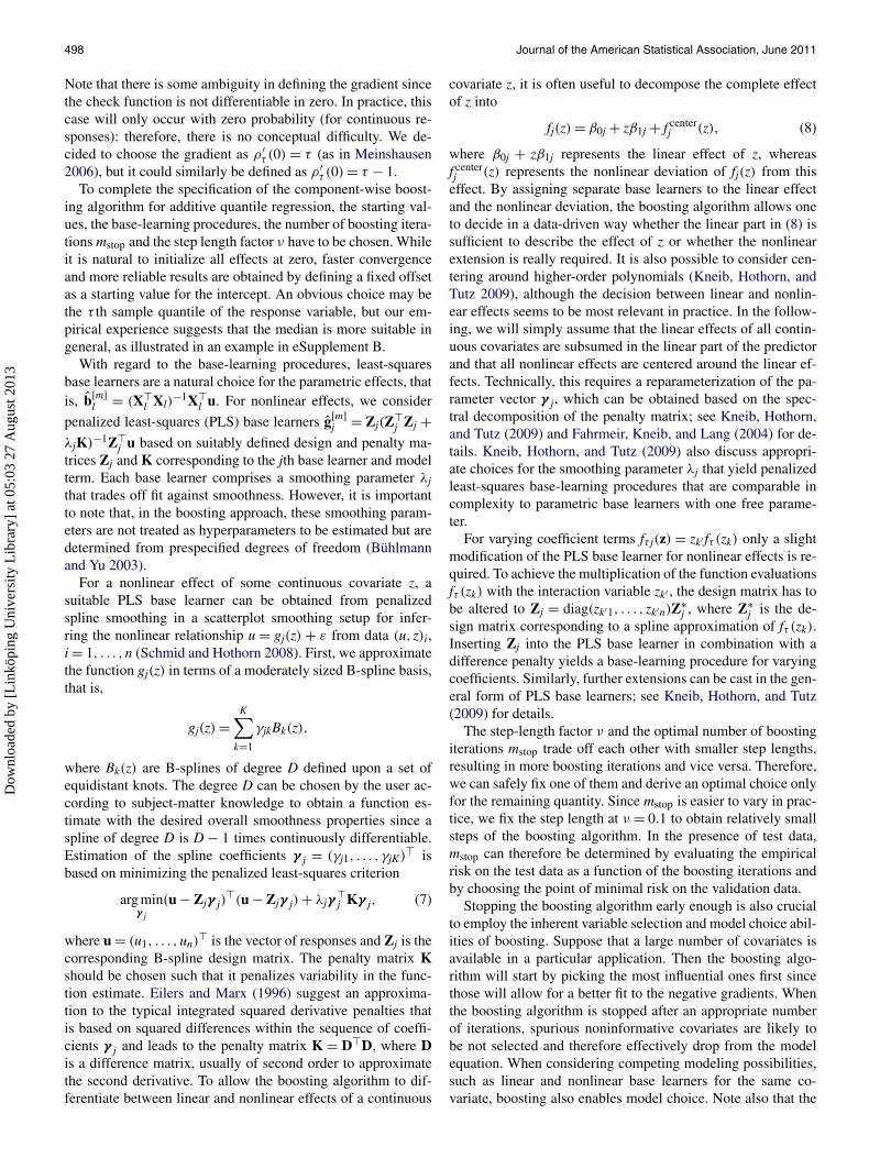
ing algorithm for additive quantile regression, the starting val-ues, the base-learning procedures, the number of boosting itera-tions mstop and the step length factor ν have to be chosen. Whileit is natural to initialize all effects at zero, faster convergenceand more reliable results are obtained by defining a fixed offsetas a starting value for the intercept. An obvious choice may bethe τ th sample quantile of the response variable, but our em-pirical experience suggests that the median is more suitable ingeneral, as illustrated in an example in eSupplement B.

With regard to the base-learning procedures, least-squaresbase learners are a natural choice for the parametric effects, thatis, b[m]

l = (X�l Xl)

−1X�l u. For nonlinear effects, we consider

penalized least-squares (PLS) base learners g[m]j = Zj(Z�

j Zj +λjK)−1Z�

j u based on suitably defined design and penalty ma-trices Zj and K corresponding to the jth base learner and modelterm. Each base learner comprises a smoothing parameter λj

that trades off fit against smoothness. However, it is importantto note that, in the boosting approach, these smoothing param-eters are not treated as hyperparameters to be estimated but aredetermined from prespecified degrees of freedom (Bühlmannand Yu 2003).

For a nonlinear effect of some continuous covariate z, asuitable PLS base learner can be obtained from penalizedspline smoothing in a scatterplot smoothing setup for infer-ring the nonlinear relationship u = gj(z) + ε from data (u, z)i,i = 1, . . . ,n (Schmid and Hothorn 2008). First, we approximatethe function gj(z) in terms of a moderately sized B-spline basis,that is,

gj(z) =K∑

k=1

γjkBk(z),

where Bk(z) are B-splines of degree D defined upon a set ofequidistant knots. The degree D can be chosen by the user ac-cording to subject-matter knowledge to obtain a function es-timate with the desired overall smoothness properties since aspline of degree D is D − 1 times continuously differentiable.Estimation of the spline coefficients γ j = (γj1, . . . , γjK)� isbased on minimizing the penalized least-squares criterion

arg minγ j

(u − Zjγ j)�(u − Zjγ j) + λjγ

�j Kγ j, (7)

where u = (u1, . . . ,un)� is the vector of responses and Zj is the

corresponding B-spline design matrix. The penalty matrix Kshould be chosen such that it penalizes variability in the func-tion estimate. Eilers and Marx (1996) suggest an approxima-tion to the typical integrated squared derivative penalties thatis based on squared differences within the sequence of coeffi-cients γ j and leads to the penalty matrix K = D�D, where Dis a difference matrix, usually of second order to approximatethe second derivative. To allow the boosting algorithm to dif-ferentiate between linear and nonlinear effects of a continuous

covariate z, it is often useful to decompose the complete effectof z into

fj(z) = β0j + zβ1j + f centerj (z), (8)

where β0j + zβ1j represents the linear effect of z, whereasf centerj (z) represents the nonlinear deviation of fj(z) from this

effect. By assigning separate base learners to the linear effectand the nonlinear deviation, the boosting algorithm allows oneto decide in a data-driven way whether the linear part in (8) issufficient to describe the effect of z or whether the nonlinearextension is really required. It is also possible to consider cen-tering around higher-order polynomials (Kneib, Hothorn, andTutz 2009), although the decision between linear and nonlin-ear effects seems to be most relevant in practice. In the follow-ing, we will simply assume that the linear effects of all contin-uous covariates are subsumed in the linear part of the predictorand that all nonlinear effects are centered around the linear ef-fects. Technically, this requires a reparameterization of the pa-rameter vector γ j, which can be obtained based on the spec-tral decomposition of the penalty matrix; see Kneib, Hothorn,and Tutz (2009) and Fahrmeir, Kneib, and Lang (2004) for de-tails. Kneib, Hothorn, and Tutz (2009) also discuss appropri-ate choices for the smoothing parameter λj that yield penalizedleast-squares base-learning procedures that are comparable incomplexity to parametric base learners with one free parame-ter.

For varying coefficient terms fτ j(z) = zk′ fτ (zk) only a slightmodification of the PLS base learner for nonlinear effects is re-quired. To achieve the multiplication of the function evaluationsfτ (zk) with the interaction variable zk′ , the design matrix has tobe altered to Zj = diag(zk′1, . . . , zk′n)Z∗

j , where Z∗j is the de-

sign matrix corresponding to a spline approximation of fτ (zk).Inserting Zj into the PLS base learner in combination with adifference penalty yields a base-learning procedure for varyingcoefficients. Similarly, further extensions can be cast in the gen-eral form of PLS base learners; see Kneib, Hothorn, and Tutz(2009) for details.

The step-length factor ν and the optimal number of boostingiterations mstop trade off each other with smaller step lengths,resulting in more boosting iterations and vice versa. Therefore,we can safely fix one of them and derive an optimal choice onlyfor the remaining quantity. Since mstop is easier to vary in prac-tice, we fix the step length at ν = 0.1 to obtain relatively smallsteps of the boosting algorithm. In the presence of test data,mstop can therefore be determined by evaluating the empiricalrisk on the test data as a function of the boosting iterations andby choosing the point of minimal risk on the validation data.

Stopping the boosting algorithm early enough is also crucialto employ the inherent variable selection and model choice abil-ities of boosting. Suppose that a large number of covariates isavailable in a particular application. Then the boosting algo-rithm will start by picking the most influential ones first sincethose will allow for a better fit to the negative gradients. Whenthe boosting algorithm is stopped after an appropriate numberof iterations, spurious noninformative covariates are likely tobe not selected and therefore effectively drop from the modelequation. When considering competing modeling possibilities,such as linear and nonlinear base learners for the same co-variate, boosting also enables model choice. Note also that the

Dow

nloa

ded

by [

Lin

köpi

ng U

nive

rsity

Lib

rary

] at

05:

03 2

7 A

ugus

t 201

3

Fenske, Kneib, and Hothorn: Identifying Risk Factors for Severe Childhood Malnutrition 499

component-wise boosting approach with separate base learnersfor the different effects allows candidate models to be set upthat may even contain more model terms than observations.

From a theoretical point of view, the Bayes consistency andconsistency of variable selection should be discussed. Notethat boosting with early stopping is a shrinkage method withimplicit penalty. Therefore, boosting estimates will be biasedfor finite samples, but typically the bias vanishes for increas-ing sample sizes. For a quadratic loss function, Bühlmann andYu (2003) showed that the optimal minimax rate is achievedby component-wise boosting with smoothing splines as baselearners. Under rather weak assumptions, Zhang and Yu (2005)showed that models fitted using a boosting algorithm with earlystopping attain the Bayes risk. Unfortunately, the results arenot directly applicable here since the check function is nottwice continuously differentiable with respect to η, and an ap-proximation by means of a continuously differentiable functionwould have to be applied. An alternative provide expectiles thatconsider an asymmetrically weighted least-squares loss func-tion (Schnabel and Eilers 2009), leading to a similar character-ization of the conditional distribution as with quantile regres-sion but with the advantage of a continuously differentiable lossfunction.

With regard to consistent variable selection, Bühlmann(2006) studied boosting for linear models, that is, with simplelinear models as base learners showing that the procedure yieldsconsistent estimates for high-dimensional problems. There areno similar results available for additive models to the best of ourknowledge. We therefore apply a stability selection procedureof Meinshausen and Bühlmann (2010), which leads to consis-tent variable selection and control of the family-wise error rate.

3. EMPIRICAL EVALUATIONS

The main goals of the empirical investigations presented herewere (i) to evaluate the correctness of both the boosting algo-rithm and its specific implementation on which our subsequentanalysis of childhood malnutrition is based on, (ii) to evaluatethe variable selection and model choice properties in higher-dimensional settings, and (iii) to judge the quality of estimatedquantile functions. For the first goal, we considered typical ad-ditive model structures with a moderate number of nonlineareffects while for the second goal we added several nuisancecovariates that actually do not impact the response but werestill considered as candidate covariates during estimation (Sec-tion 3.1). Finally, we compared the estimated quantile functionsdirectly with the true underlying quantile function in a simpleunivariate setup (Section 3.2).

3.1 Comparing Empirical Risks

Basic Model. The basic model specification for the empiri-cal investigations is

yi = β0 + f1(zi1) + · · · + fq(ziq)

+ [α0 + g1(zi1) + · · · + gq(ziq)]εi, where εiiid∼ H. (9)

Here, the location and the scale of the response yi can dependin nonlinear form on covariates zi1, . . . , ziq and an error termεi with distribution function H not depending on covariates.Choosing all fj and gj as linear functions yields a linear model:

see eSupplement B. If functions fj and gj are zero, the associ-ated covariates have no influence on the response. The resultingquantile function has a nonlinear predictor structure and can bewritten as

QYi(τ |zi) = β0 + f1(zi1) + · · · + fq(ziq)

+ H−1(τ )[α0 + g1(zi1) + · · · + gq(ziq)].Based on the additive model in (9), we considered the followingtwo univariable setups:

q = 1 β0 f1(zi1) α0 g1(zi1)

‘sin’-setup: 2 1.5 sin( 23 zi1) 0.5 1.5z2

i1‘log’-setup: 2 1.5 log(zi1 + 1.05) 1 0.7zi1

and a multivariable setup with q = 6:

β0 2 α0 0.5f1(zi1) 1.5 sin( 2

3 zi1) g1(zi1) 0.5z2i1

f2(zi2) 1.5 log(zi2 + 1.05) g2(zi2) 0.5zi2f3(zi3) 2zi3 g3(zi3) 0.5zi3f4(zi4) −2zi4 g4(zi4) 0f5(zi5) 0 g5(zi5) 0f6(zi6) 0 g6(zi6) 0

In the multivariable setup, two covariates relate nonlinearlyto the response, two have a linear influence on it, and the lasttwo have no influence at all.

For generating datasets based on these variable setups, co-variates zi were drawn from a uniform distribution U [0,1]with a Toeplitz-structured covariance matrix, leading to cov(zik,

zil) = ρ|k−l| for possible correlation coefficients ρ ∈ {0,0.2,

0.5,0.8}. Also, we repeated each setup for different distri-butions of the error term: a standard normal, a t distribu-tion with two degrees of freedom, and a gamma distribution,where E(εi) = V(εi) = 2. Figure 1 shows data examples from‘sin’- and ‘log’-setups for normal- and gamma-distributed errorterms.

For each parameter combination consisting of a specific vari-able setup, correlation coefficient, and error distribution, wegenerated three independent datasets: A validation dataset con-sisting of 200 observations to select optional tuning parameters,a training dataset with 400 observations for model estimation,and a test dataset with 1000 observations to evaluate the perfor-mance of each algorithm.

Estimation. We estimated additive quantile regression mod-els for each parameter setup with potential nonlinear ef-fects for all covariates on a fixed quantile grid with τ ∈{0.1,0.3,0.5,0.7,0.9}. We used five different estimation al-gorithms: additive quantile boosting (gamboost), total vari-ation regularization (rqss, Koenker, Ng, and Portnoy 1994),boosting with stump base learners (stumps, Kriegler andBerk 2010), boosting with higher-order tree base learners(trees, Kriegler and Berk 2010), and quantile regressionforests (quantregForest, Meinshausen 2006). In the caseof gamboost, we used cubic-penalized spline base learnerswith a second-order difference penalty, 20 inner knots, five de-grees of freedom, and fixed the step length at ν = 0.1. The

Dow

nloa

ded

by [

Lin

köpi

ng U

nive

rsity

Lib

rary

] at

05:

03 2

7 A

ugus

t 201

3

500 Journal of the American Statistical Association, June 2011

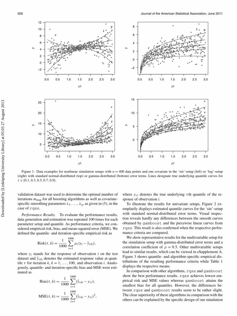
Figure 1. Data examples for nonlinear simulation setups with n = 400 data points and one covariate in the ‘sin’-setup (left) or ‘log’-setup(right) with standard normal-distributed (top) or gamma-distributed (bottom) error terms. Lines designate true underlying quantile curves forτ ∈ {0.1,0.3,0.5,0.7,0.9}.

validation dataset was used to determine the optimal number ofiterations mstop for all boosting algorithms as well as covariate-specific smoothing parameters λ1, . . . , λq, as given in (5), in thecase of rqss.

Performance Results. To evaluate the performance results,data generation and estimation was repeated 100 times for eachparameter setup and quantile. As performance criteria, we con-sidered empirical risk, bias, and mean-squared error (MSE). Wedefined the quantile- and iteration-specific empirical risk as

Risk(τ, k) = 1

1000

1000∑i=1

ρτ (yi − yτki),

where yi stands for the response of observation i on the testdataset and yτki denotes the estimated response value at quan-tile τ for iteration k, k = 1, . . . ,100, and observation i. Analo-gously, quantile- and iteration-specific bias and MSE were esti-mated as

Bias(τ, k) = 1

1000

1000∑i=1

(yτki − yτ i),

MSE(τ, k) = 1

1000

1000∑i=1

(yτki − yτ i)2,

where yτ i denotes the true underlying τ th quantile of the re-sponse of observation i.

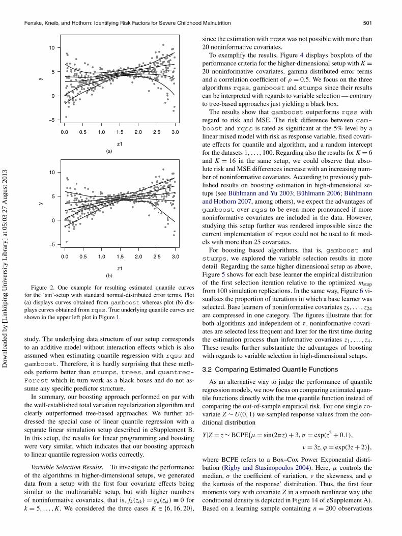
To illustrate the results for univariate setups, Figure 2 ex-emplarily displays estimated quantile curves for the ‘sin’-setupwith standard normal-distributed error terms. Visual inspec-tion reveals hardly any differences between the smooth curvesobtained by gamboost and the piecewise linear curves fromrqss. This result is also confirmed when the respective perfor-mance criteria are compared.

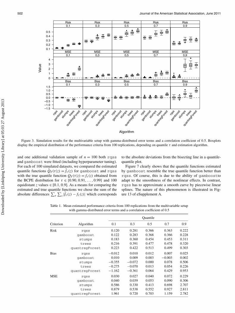
We show representative results for the multivariable setup forthe simulation setup with gamma-distributed error terms and acorrelation coefficient of ρ = 0.5. Other multivariable setupslead to similar results, which can be viewed in eSupplement A.Figure 3 shows quantile- and algorithm-specific empirical dis-tributions of the resulting performance criteria while Table 1displays the respective means.

In comparison with other algorithms, rqss and gamboostshow the best performance results. rqss achieves lowest em-pirical risk and MSE values whereas gamboost attains thesmallest bias for all quantiles. However, the differences be-tween rqss and gamboost results seem to be rather slight.The clear superiority of these algorithms in comparison with theothers can be explained by the specific design of our simulation

Dow

nloa

ded

by [

Lin

köpi

ng U

nive

rsity

Lib

rary

] at

05:

03 2

7 A

ugus

t 201

3

Fenske, Kneib, and Hothorn: Identifying Risk Factors for Severe Childhood Malnutrition 501

(a)

(b)

Figure 2. One example for resulting estimated quantile curvesfor the ‘sin’-setup with standard normal-distributed error terms. Plot(a) displays curves obtained from gamboost whereas plot (b) dis-plays curves obtained from rqss. True underlying quantile curves areshown in the upper left plot in Figure 1.

study. The underlying data structure of our setup correspondsto an additive model without interaction effects which is alsoassumed when estimating quantile regression with rqss andgamboost. Therefore, it is hardly surprising that these meth-ods perform better than stumps, trees, and quantreg-Forest which in turn work as a black boxes and do not as-sume any specific predictor structure.

In summary, our boosting approach performed on par withthe well-established total variation regularization algorithm andclearly outperformed tree-based approaches. We further ad-dressed the special case of linear quantile regression with aseparate linear simulation setup described in eSupplement B.In this setup, the results for linear programming and boostingwere very similar, which indicates that our boosting approachto linear quantile regression works correctly.

Variable Selection Results. To investigate the performanceof the algorithms in higher-dimensional setups, we generateddata from a setup with the first four covariate effects beingsimilar to the multivariable setup, but with higher numbersof noninformative covariates, that is, fk(zik) = gk(zik) ≡ 0 fork = 5, . . . ,K. We considered the three cases K ∈ {6,16,20},

since the estimation with rqsswas not possible with more than20 noninformative covariates.

To exemplify the results, Figure 4 displays boxplots of theperformance criteria for the higher-dimensional setup with K =20 noninformative covariates, gamma-distributed error termsand a correlation coefficient of ρ = 0.5. We focus on the threealgorithms rqss, gamboost and stumps since their resultscan be interpreted with regards to variable selection — contraryto tree-based approaches just yielding a black box.

The results show that gamboost outperforms rqss withregard to risk and MSE. The risk difference between gam-boost and rqss is rated as significant at the 5% level by alinear mixed model with risk as response variable, fixed covari-ate effects for quantile and algorithm, and a random interceptfor the datasets 1, . . . ,100. Regarding also the results for K = 6and K = 16 in the same setup, we could observe that abso-lute risk and MSE differences increase with an increasing num-ber of noninformative covariates. According to previously pub-lished results on boosting estimation in high-dimensional se-tups (see Bühlmann and Yu 2003; Bühlmann 2006; Bühlmannand Hothorn 2007, among others), we expect the advantages ofgamboost over rqss to be even more pronounced if morenoninformative covariates are included in the data. However,studying this setup further was rendered impossible since thecurrent implementation of rqss could not be used to fit mod-els with more than 25 covariates.

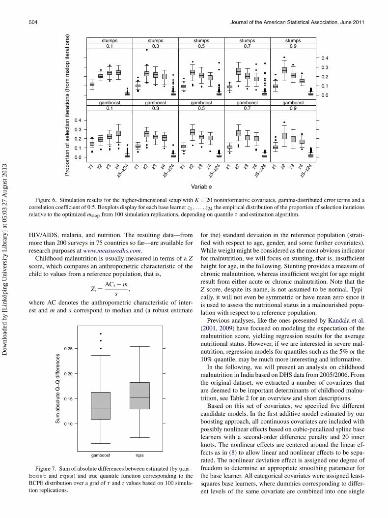
For boosting based algorithms, that is, gamboost andstumps, we explored the variable selection results in moredetail. Regarding the same higher-dimensional setup as above,Figure 5 shows for each base learner the empirical distributionof the first selection iteration relative to the optimized mstopfrom 100 simulation replications. In the same way, Figure 6 vi-sualizes the proportion of iterations in which a base learner wasselected. Base learners of noninformative covariates z5, . . . , z24are compressed in one category. The figures illustrate that forboth algorithms and independent of τ , noninformative covari-ates are selected less frequent and later for the first time duringthe estimation process than informative covariates z1, . . . , z4.These results further substantiate the advantages of boostingwith regards to variable selection in high-dimensional setups.

3.2 Comparing Estimated Quantile Functions

As an alternative way to judge the performance of quantileregression models, we now focus on comparing estimated quan-tile functions directly with the true quantile function instead ofcomparing the out-of-sample empirical risk. For one single co-variate Z ∼ U(0,1) we sampled response values from the con-ditional distribution

Y|Z = z ∼ BCPE(μ = sin(2πz) + 3, σ = exp(z2 + 0.1),

ν = 3z, ϕ = exp(3z + 2)),

where BCPE refers to a Box–Cox Power Exponential distri-bution (Rigby and Stasinopoulos 2004). Here, μ controls themedian, σ the coefficient of variation, ν the skewness, and ϕ

the kurtosis of the response’ distribution. Thus, the first fourmoments vary with covariate Z in a smooth nonlinear way (theconditional density is depicted in Figure 14 of eSupplement A).Based on a learning sample containing n = 200 observations

Dow

nloa

ded

by [

Lin

köpi

ng U

nive

rsity

Lib

rary

] at

05:

03 2

7 A

ugus

t 201

3

502 Journal of the American Statistical Association, June 2011

Figure 3. Simulation results for the multivariable setup with gamma-distributed error terms and a correlation coefficient of 0.5. Boxplotsdisplay the empirical distribution of the performance criteria from 100 replications, depending on quantile τ and estimation algorithm.

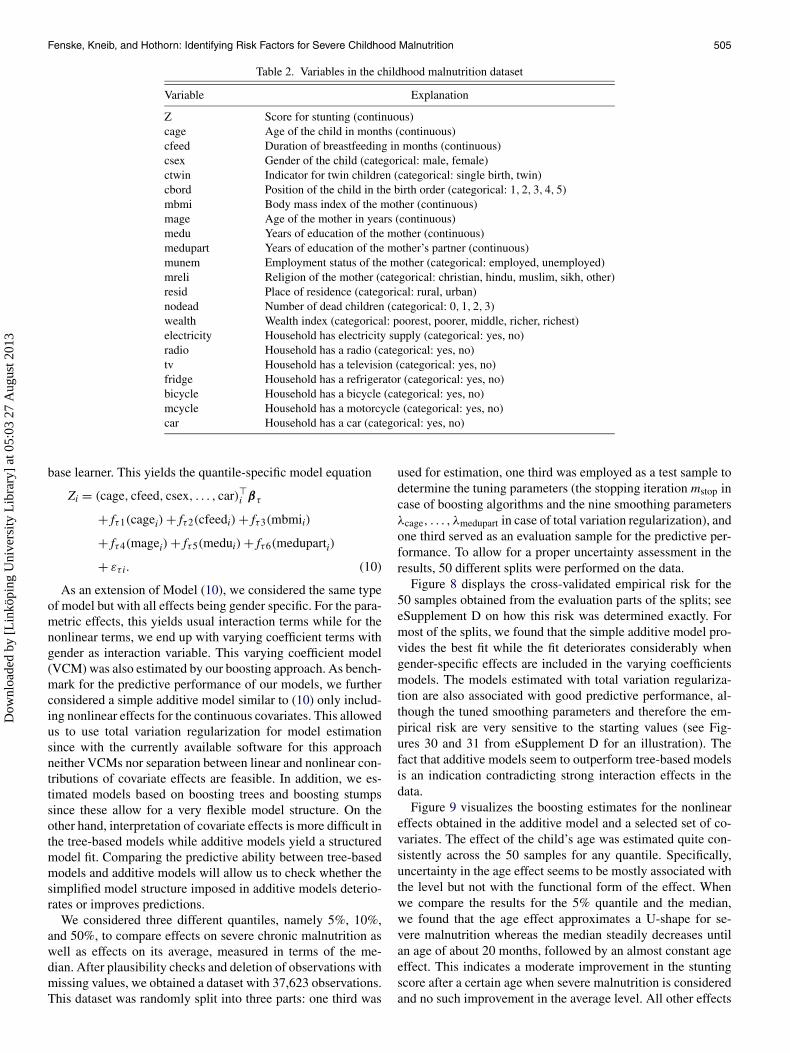
and one additional validation sample of n = 100 both rqssand gamboost were fitted (including hyperparameter tuning).For each of 100 simulated datasets, we compared the estimatedquantile functions QY(τ |z) = fτ (z) for gamboost and rqsswith the true quantile function QY(τ |z) = fτ (z) obtained fromthe BCPE distribution for τ ∈ {0.90,0.91, . . . ,0.99} and 100equidistant z values ∈ [0.1,0.9]. As a means for comparing theestimated and true quantile functions we chose the sum of theabsolute differences

∑τ

∑z |fτ (z) − fτ (z)| which corresponds

to the absolute deviations from the bisecting line in a quantile-quantile plot.

Figure 7 clearly shows that the quantile functions estimatedby gamboost resemble the true quantile function better thanrqss. Of course, this is due to the ability of gamboosttoadapt to the smoothness of the nonlinear effects. In contrast,rqss has to approximate a smooth curve by piecewise linearsplines. The nature of this phenomenon is illustrated in Fig-ure 13 of eSupplement A.

Table 1. Mean estimated performance criteria from 100 replications from the multivariable setupwith gamma-distributed error terms and a correlation coefficient of 0.5

Quantile

Criterion Algorithm 0.1 0.3 0.5 0.7 0.9

Risk rqss 0.120 0.281 0.366 0.363 0.222gamboost 0.122 0.283 0.368 0.366 0.228stumps 0.183 0.360 0.454 0.453 0.311trees 0.216 0.391 0.477 0.478 0.320

quantregForest 0.223 0.422 0.513 0.499 0.303

Bias rqss −0.012 0.010 0.012 0.007 0.025gamboost 0.010 0.009 0.003 −0.003 0.002stumps −0.355 −0.072 0.000 0.078 0.506trees −0.275 −0.070 0.013 0.054 0.226

quantregForest −1.162 −0.361 0.064 0.429 0.953

MSE rqss 0.030 0.027 0.040 0.072 0.229gamboost 0.040 0.039 0.053 0.090 0.306stumps 0.586 0.330 0.413 0.698 2.707trees 0.879 0.538 0.552 0.927 2.811

quantregForest 1.961 0.720 0.703 1.159 2.782

Dow

nloa

ded

by [

Lin

köpi

ng U

nive

rsity

Lib

rary

] at

05:

03 2

7 A

ugus

t 201

3

Fenske, Kneib, and Hothorn: Identifying Risk Factors for Severe Childhood Malnutrition 503

Figure 4. Simulation results for the higher-dimensional setup with K = 20 noninformative covariates, gamma-distributed error terms and acorrelation coefficient of 0.5. Boxplots display empirical distributions of the performance criteria from 100 replications, depending on quantileτ and three estimation algorithms.

4. ANALYZING CHILDHOOD MALNUTRITION IN INDIA

Childhood malnutrition is one of the most urgent problems

in developing and transition countries. To provide information

not only on the nutritional status but also on health and popula-tion trends in general, Demographic and Health Surveys (DHS)conduct nationally representative surveys on fertility, familyplanning, maternal and child health, as well as child survival,

Figure 5. Simulation results for the higher-dimensional setup with K = 20 noninformative covariates, gamma-distributed error terms and acorrelation coefficient of 0.5. Boxplots display for each base learner z1, . . . , z24 the empirical distribution of the first selection iteration relativeto the optimized mstop from 100 simulation replications, depending on quantile τ and estimation algorithm.

Dow

nloa

ded

by [

Lin

köpi

ng U

nive

rsity

Lib

rary

] at

05:

03 2

7 A

ugus

t 201

3

504 Journal of the American Statistical Association, June 2011

Figure 6. Simulation results for the higher-dimensional setup with K = 20 noninformative covariates, gamma-distributed error terms and acorrelation coefficient of 0.5. Boxplots display for each base learner z1, . . . , z24 the empirical distribution of the proportion of selection iterationsrelative to the optimized mstop from 100 simulation replications, depending on quantile τ and estimation algorithm.

HIV/AIDS, malaria, and nutrition. The resulting data—frommore than 200 surveys in 75 countries so far—are available forresearch purposes at www.measuredhs.com.

Childhood malnutrition is usually measured in terms of a Zscore, which compares an anthropometric characteristic of thechild to values from a reference population, that is,

Zi = ACi − m

s,

where AC denotes the anthropometric characteristic of inter-est and m and s correspond to median and (a robust estimate

Figure 7. Sum of absolute differences between estimated (by gam-boost and rqss) and true quantile function corresponding to theBCPE distribution over a grid of τ and z values based on 100 simula-tion replications.

for the) standard deviation in the reference population (strati-fied with respect to age, gender, and some further covariates).While weight might be considered as the most obvious indicatorfor malnutrition, we will focus on stunting, that is, insufficientheight for age, in the following. Stunting provides a measure ofchronic malnutrition, whereas insufficient weight for age mightresult from either acute or chronic malnutrition. Note that theZ score, despite its name, is not assumed to be normal. Typi-cally, it will not even be symmetric or have mean zero since itis used to assess the nutritional status in a malnourished popu-lation with respect to a reference population.

Previous analyses, like the ones presented by Kandala et al.(2001, 2009) have focused on modeling the expectation of themalnutrition score, yielding regression results for the averagenutritional status. However, if we are interested in severe mal-nutrition, regression models for quantiles such as the 5% or the10% quantile, may be much more interesting and informative.

In the following, we will present an analysis on childhoodmalnutrition in India based on DHS data from 2005/2006. Fromthe original dataset, we extracted a number of covariates thatare deemed to be important determinants of childhood malnu-trition, see Table 2 for an overview and short descriptions.

Based on this set of covariates, we specified five differentcandidate models. In the first additive model estimated by ourboosting approach, all continuous covariates are included withpossibly nonlinear effects based on cubic-penalized spline baselearners with a second-order difference penalty and 20 innerknots. The nonlinear effects are centered around the linear ef-fects as in (8) to allow linear and nonlinear effects to be sepa-rated. The nonlinear deviation effect is assigned one degree offreedom to determine an appropriate smoothing parameter forthe base learner. All categorical covariates were assigned least-squares base learners, where dummies corresponding to differ-ent levels of the same covariate are combined into one single

Dow

nloa

ded

by [

Lin

köpi

ng U

nive

rsity

Lib

rary

] at

05:

03 2

7 A

ugus

t 201

3

Fenske, Kneib, and Hothorn: Identifying Risk Factors for Severe Childhood Malnutrition 505

Table 2. Variables in the childhood malnutrition dataset

Variable Explanation

Z Score for stunting (continuous)cage Age of the child in months (continuous)cfeed Duration of breastfeeding in months (continuous)csex Gender of the child (categorical: male, female)ctwin Indicator for twin children (categorical: single birth, twin)cbord Position of the child in the birth order (categorical: 1,2,3,4,5)mbmi Body mass index of the mother (continuous)mage Age of the mother in years (continuous)medu Years of education of the mother (continuous)medupart Years of education of the mother’s partner (continuous)munem Employment status of the mother (categorical: employed, unemployed)mreli Religion of the mother (categorical: christian, hindu, muslim, sikh, other)resid Place of residence (categorical: rural, urban)nodead Number of dead children (categorical: 0,1,2,3)wealth Wealth index (categorical: poorest, poorer, middle, richer, richest)electricity Household has electricity supply (categorical: yes, no)radio Household has a radio (categorical: yes, no)tv Household has a television (categorical: yes, no)fridge Household has a refrigerator (categorical: yes, no)bicycle Household has a bicycle (categorical: yes, no)mcycle Household has a motorcycle (categorical: yes, no)car Household has a car (categorical: yes, no)

base learner. This yields the quantile-specific model equation

Zi = (cage, cfeed, csex, . . . , car)�i βτ

+ fτ1(cagei) + fτ2(cfeedi) + fτ3(mbmii)

+ fτ4(magei) + fτ5(medui) + fτ6(meduparti)

+ ετ i. (10)

As an extension of Model (10), we considered the same typeof model but with all effects being gender specific. For the para-metric effects, this yields usual interaction terms while for thenonlinear terms, we end up with varying coefficient terms withgender as interaction variable. This varying coefficient model(VCM) was also estimated by our boosting approach. As bench-mark for the predictive performance of our models, we furtherconsidered a simple additive model similar to (10) only includ-ing nonlinear effects for the continuous covariates. This allowedus to use total variation regularization for model estimationsince with the currently available software for this approachneither VCMs nor separation between linear and nonlinear con-tributions of covariate effects are feasible. In addition, we es-timated models based on boosting trees and boosting stumpssince these allow for a very flexible model structure. On theother hand, interpretation of covariate effects is more difficult inthe tree-based models while additive models yield a structuredmodel fit. Comparing the predictive ability between tree-basedmodels and additive models will allow us to check whether thesimplified model structure imposed in additive models deterio-rates or improves predictions.

We considered three different quantiles, namely 5%, 10%,and 50%, to compare effects on severe chronic malnutrition aswell as effects on its average, measured in terms of the me-dian. After plausibility checks and deletion of observations withmissing values, we obtained a dataset with 37,623 observations.This dataset was randomly split into three parts: one third was

used for estimation, one third was employed as a test sample todetermine the tuning parameters (the stopping iteration mstop incase of boosting algorithms and the nine smoothing parametersλcage, . . . , λmedupart in case of total variation regularization), andone third served as an evaluation sample for the predictive per-formance. To allow for a proper uncertainty assessment in theresults, 50 different splits were performed on the data.

Figure 8 displays the cross-validated empirical risk for the50 samples obtained from the evaluation parts of the splits; seeeSupplement D on how this risk was determined exactly. Formost of the splits, we found that the simple additive model pro-vides the best fit while the fit deteriorates considerably whengender-specific effects are included in the varying coefficientsmodels. The models estimated with total variation regulariza-tion are also associated with good predictive performance, al-though the tuned smoothing parameters and therefore the em-pirical risk are very sensitive to the starting values (see Fig-ures 30 and 31 from eSupplement D for an illustration). Thefact that additive models seem to outperform tree-based modelsis an indication contradicting strong interaction effects in thedata.

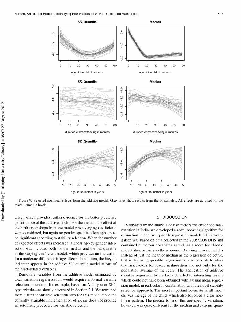
Figure 9 visualizes the boosting estimates for the nonlineareffects obtained in the additive model and a selected set of co-variates. The effect of the child’s age was estimated quite con-sistently across the 50 samples for any quantile. Specifically,uncertainty in the age effect seems to be mostly associated withthe level but not with the functional form of the effect. Whenwe compare the results for the 5% quantile and the median,we found that the age effect approximates a U-shape for se-vere malnutrition whereas the median steadily decreases untilan age of about 20 months, followed by an almost constant ageeffect. This indicates a moderate improvement in the stuntingscore after a certain age when severe malnutrition is consideredand no such improvement in the average level. All other effects

Dow

nloa

ded

by [

Lin

köpi

ng U

nive

rsity

Lib

rary

] at

05:

03 2

7 A

ugus

t 201

3

506 Journal of the American Statistical Association, June 2011

Figure 8. Boxplots display empirical distributions of the cross-validated empirical risks for the evaluation parts of the 50 data splits. Resultsfor one split are connected by gray lines.

are associated with a much stronger uncertainty and less clearpatterns across the 50 samples. For example, the effect of theduration of breastfeeding considerably varies in the functionalform, in particular for the median. Here we also find a moderatedecrease in the stunting score, while there seems to be almostno effect on the 5% quantile. Similarly, the age of the motherhas a somewhat nonlinear effect on the median, but is closer toa linear effect for the 5% quantile.

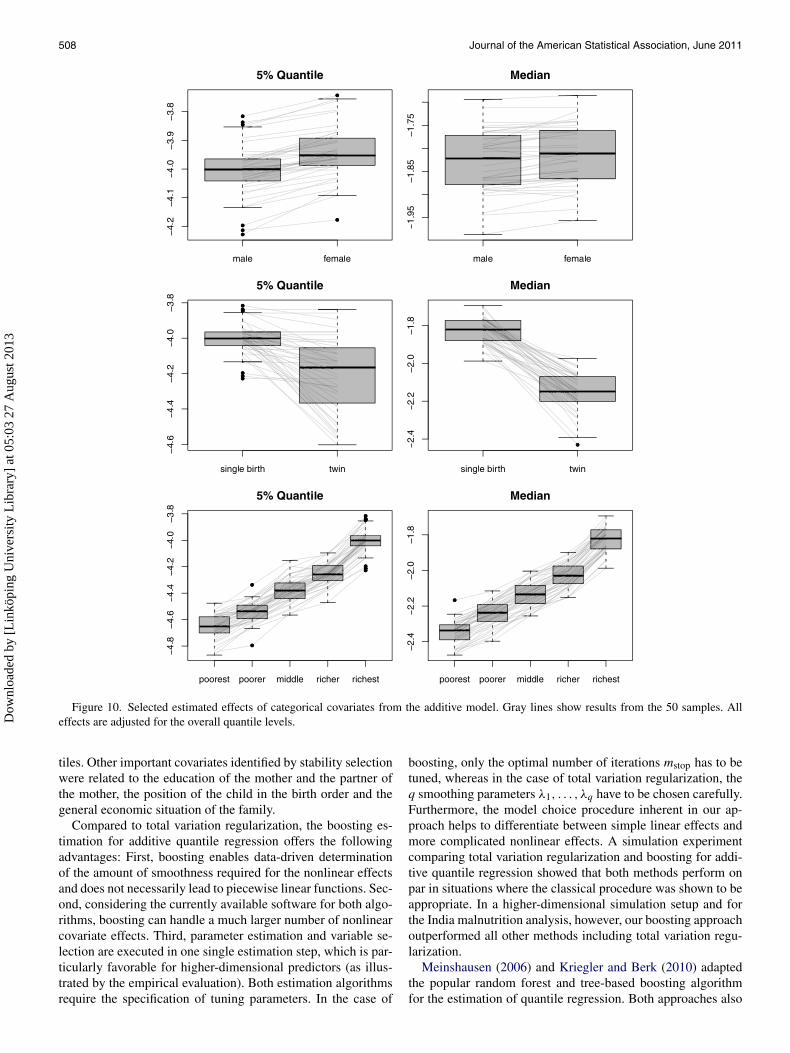
Results for some selected effects of categorical covariates ob-tained in the additive model are shown in Figure 10. We founda clear indication, consistent across all quantiles, that a betternutritional status is associated with richer families. Similarly, abetter nutritional status is associated with single births as com-pared to twin births, which seems plausible since in a twin birthtwo children are competing for fixed resources. Note that thetwin effect is actually much stronger for the median, where theestimated effects are quite expressed in every replication, whichleads to almost separated levels for twin and single births. Forthe gender effect, we found a moderate preference for femalechildren, which was more prominent for the 5% quantile. Com-plete results for all covariate effects obtained in the additiveboosting approach can be found in eSupplement C.

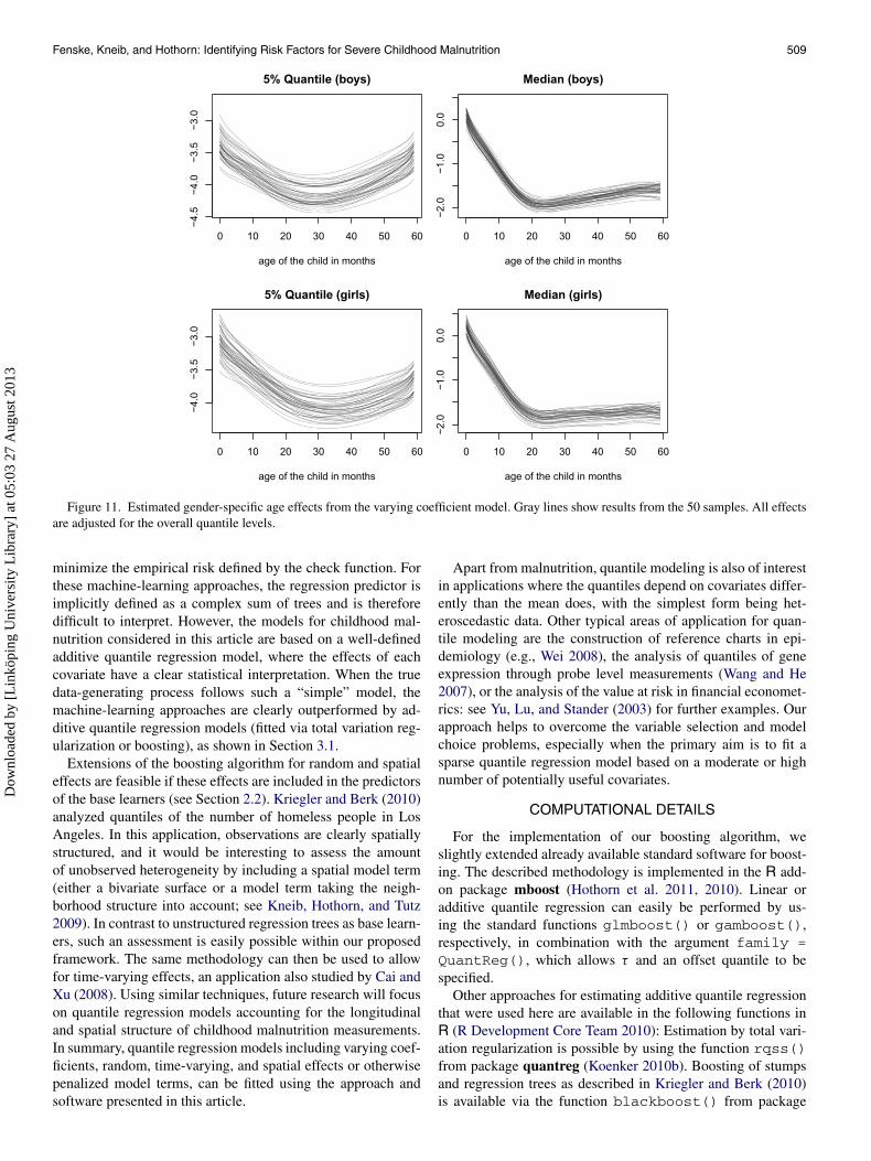
For illustrative purposes, we also show one selected effectfrom the varying coefficient model, although we have foundthat it does not have the same predictive ability as the additivemodel. Figure 11 shows the gender-specific age effect, and re-veals qualitatively similar differences between the 5% quantileand the median for both boys and girls. However, some interest-ing differences become apparent when one looks more closely

at the precise shape of the functions. For the 5% quantile, theimprovement in the stunting score after and at the age of about30 months is less prominent for girls. For boys, in contrast, theage effect on the 5% quantile is almost symmetric about 30months. Similarly, for boys, there is a moderate improvementafter an age of 20 months in the median effect for boys, but thiseffect is much less expressed, or even absent, for girls.

Finally, we addressed the inference problem in the additivemodel more formally based on the stability selection procedureproposed by Meinshausen and Bühlmann (2010), which allowsthe family-wise error rate in model choice to be controlled sim-ilarly as usual significance tests control the Type I error. Thebasic idea is to fix an average number of terms to be expectedin a model and an upper bound for the family-wise error rate.The stability selection procedure then provides a threshold forthe relative frequency of a model term to be among the firstterms selected in the boosting procedure. We chose an averagenumber of ten terms and a family-wise error rate of 5% in thefollowing, but the results were almost insensitive with respectto changes in the expected number of terms. For an additivemodel and the 5% quantile, a nonlinear effect of the child’sage and linear effects of the birth order, the wealth indicator,and the educational level of both the mother and the mother’spartner had a “significant” impact on the nutritional status. Forthe additive median model, also linear effects of the durationof breastfeeding and the body mass index of the mother werefound. When varying coefficient models were considered, ex-actly the same effects for the 5% quantile were found as withthe additive model. In particular, there was no gender-specific

Dow

nloa

ded

by [

Lin

köpi

ng U

nive

rsity

Lib

rary

] at

05:

03 2

7 A

ugus

t 201

3

Fenske, Kneib, and Hothorn: Identifying Risk Factors for Severe Childhood Malnutrition 507

Figure 9. Selected nonlinear effects from the additive model. Gray lines show results from the 50 samples. All effects are adjusted for theoverall quantile levels.

effect, which provides further evidence for the better predictiveperformance of the additive model. For the median, the effect ofthe birth order drops from the model when varying coefficientswere considered, but again no gender-specific effect appears tobe significant according to stability selection. When the numberof expected effects was increased, a linear age-by-gender inter-action was included both for the median and the 5% quantilein the varying coefficient model, which provides an indicationfor a moderate difference in age effects. In addition, the bicycleindicator appears in the additive 5% quantile model as one ofthe asset-related variables.

Removing variables from the additive model estimated bytotal variation regularization would require a formal variableselection procedure, for example, based on AIC-type or SIC-type criteria—as shortly discussed in Section 2.1. We refrainedfrom a further variable selection step for this model since thecurrently available implementation of rqss does not providean automatic procedure for variable selection.

5. DISCUSSION

Motivated by the analysis of risk factors for childhood mal-nutrition in India, we developed a novel boosting algorithm forestimation in additive quantile regression models. Our investi-gation was based on data collected in the 2005/2006 DHS andcontained numerous covariates as well as a score for chronicmalnutrition serving as the response. By using lower quantilesinstead of just the mean or median as the regression objective,that is, by using quantile regression, it was possible to iden-tify risk factors for severe malnutrition and not only for thepopulation average of the score. The application of additivequantile regression to the India data led to interesting resultswhich could not have been obtained with a usual mean regres-sion model, in particular in combination with the novel stabilityselection approach. The most important covariate in all mod-els was the age of the child, which also followed a clear non-linear pattern. The precise form of this age-specific variation,however, was quite different for the median and extreme quan-

Dow

nloa

ded

by [

Lin

köpi

ng U

nive

rsity

Lib

rary

] at

05:

03 2

7 A

ugus

t 201

3

508 Journal of the American Statistical Association, June 2011

Figure 10. Selected estimated effects of categorical covariates from the additive model. Gray lines show results from the 50 samples. Alleffects are adjusted for the overall quantile levels.

tiles. Other important covariates identified by stability selectionwere related to the education of the mother and the partner ofthe mother, the position of the child in the birth order and thegeneral economic situation of the family.

Compared to total variation regularization, the boosting es-timation for additive quantile regression offers the followingadvantages: First, boosting enables data-driven determinationof the amount of smoothness required for the nonlinear effectsand does not necessarily lead to piecewise linear functions. Sec-ond, considering the currently available software for both algo-rithms, boosting can handle a much larger number of nonlinearcovariate effects. Third, parameter estimation and variable se-lection are executed in one single estimation step, which is par-ticularly favorable for higher-dimensional predictors (as illus-trated by the empirical evaluation). Both estimation algorithmsrequire the specification of tuning parameters. In the case of

boosting, only the optimal number of iterations mstop has to betuned, whereas in the case of total variation regularization, theq smoothing parameters λ1, . . . , λq have to be chosen carefully.Furthermore, the model choice procedure inherent in our ap-proach helps to differentiate between simple linear effects andmore complicated nonlinear effects. A simulation experimentcomparing total variation regularization and boosting for addi-tive quantile regression showed that both methods perform onpar in situations where the classical procedure was shown to beappropriate. In a higher-dimensional simulation setup and forthe India malnutrition analysis, however, our boosting approachoutperformed all other methods including total variation regu-larization.

Meinshausen (2006) and Kriegler and Berk (2010) adaptedthe popular random forest and tree-based boosting algorithmfor the estimation of quantile regression. Both approaches also

Dow

nloa

ded

by [

Lin

köpi

ng U

nive

rsity

Lib

rary

] at

05:

03 2

7 A

ugus

t 201

3

Fenske, Kneib, and Hothorn: Identifying Risk Factors for Severe Childhood Malnutrition 509

Figure 11. Estimated gender-specific age effects from the varying coefficient model. Gray lines show results from the 50 samples. All effectsare adjusted for the overall quantile levels.

minimize the empirical risk defined by the check function. Forthese machine-learning approaches, the regression predictor isimplicitly defined as a complex sum of trees and is thereforedifficult to interpret. However, the models for childhood mal-nutrition considered in this article are based on a well-definedadditive quantile regression model, where the effects of eachcovariate have a clear statistical interpretation. When the truedata-generating process follows such a “simple” model, themachine-learning approaches are clearly outperformed by ad-ditive quantile regression models (fitted via total variation reg-ularization or boosting), as shown in Section 3.1.

Extensions of the boosting algorithm for random and spatialeffects are feasible if these effects are included in the predictorsof the base learners (see Section 2.2). Kriegler and Berk (2010)analyzed quantiles of the number of homeless people in LosAngeles. In this application, observations are clearly spatiallystructured, and it would be interesting to assess the amountof unobserved heterogeneity by including a spatial model term(either a bivariate surface or a model term taking the neigh-borhood structure into account; see Kneib, Hothorn, and Tutz2009). In contrast to unstructured regression trees as base learn-ers, such an assessment is easily possible within our proposedframework. The same methodology can then be used to allowfor time-varying effects, an application also studied by Cai andXu (2008). Using similar techniques, future research will focuson quantile regression models accounting for the longitudinaland spatial structure of childhood malnutrition measurements.In summary, quantile regression models including varying coef-ficients, random, time-varying, and spatial effects or otherwisepenalized model terms, can be fitted using the approach andsoftware presented in this article.

Apart from malnutrition, quantile modeling is also of interestin applications where the quantiles depend on covariates differ-ently than the mean does, with the simplest form being het-eroscedastic data. Other typical areas of application for quan-tile modeling are the construction of reference charts in epi-demiology (e.g., Wei 2008), the analysis of quantiles of geneexpression through probe level measurements (Wang and He2007), or the analysis of the value at risk in financial economet-rics: see Yu, Lu, and Stander (2003) for further examples. Ourapproach helps to overcome the variable selection and modelchoice problems, especially when the primary aim is to fit asparse quantile regression model based on a moderate or highnumber of potentially useful covariates.

COMPUTATIONAL DETAILS

For the implementation of our boosting algorithm, weslightly extended already available standard software for boost-ing. The described methodology is implemented in the R add-on package mboost (Hothorn et al. 2011, 2010). Linear oradditive quantile regression can easily be performed by us-ing the standard functions glmboost() or gamboost(),respectively, in combination with the argument family =QuantReg(), which allows τ and an offset quantile to bespecified.

Other approaches for estimating additive quantile regressionthat were used here are available in the following functions inR (R Development Core Team 2010): Estimation by total vari-ation regularization is possible by using the function rqss()from package quantreg (Koenker 2010b). Boosting of stumpsand regression trees as described in Kriegler and Berk (2010)is available via the function blackboost() from package

Dow

nloa

ded

by [

Lin

köpi

ng U

nive

rsity

Lib

rary

] at

05:

03 2

7 A

ugus

t 201

3

510 Journal of the American Statistical Association, June 2011

mboost. Quantile regression forests can be estimated with thefunction quantregForest() from package quantregFor-est (Meinshausen 2007).

To assure the reproducibility of the results of our data anal-yses, we include an electronic supplement to this article thatcontains all necessary R commands to prepare and analyze theIndian malnutrition data (provided that the original dataset wasobtained from www.measuredhs.com). If package mboost (ver-sion 2.0-10 or higher) is installed, simply type

R> source(system.file("India_quantiles.R",package = "mboost"))

to reproduce our analyses.

SUPPLEMENTARY MATERIALS

Results: We provide additional results from simulation experi-ments and data analyses, and the complete source code of thesimulation experiments. (eSupplement.pdf)

[Received April 2009. Revised February 2011.]

REFERENCESAckerson, L. K., and Subramanian, S. (2008), “Domestic Violence and Chronic

Malnutrition Among Women and Children in India,” American Journal ofEpidemiology, 167, 1188–1196. [494]

Bharati, S., Pal, M., and Bharati, P. (2008), “Determinants of Nutritional Statusof Pre-School Children in India,” Journal of Biosocial Science, 40, 801–814. [494]

Buchinsky, M. (1998), “Recent Advances in Quantile Regression Models:A Practical Guideline for Empirical Research,” The Journal of Human Re-sources, 33, 88–126. [495]

Bühlmann, P. (2006), “Boosting for High-Dimensional Linear Models,” TheAnnals of Statistics, 34, 559–583. [499,501]

Bühlmann, P., and Hothorn, T. (2007), “Boosting Algorithms: Regularization,Prediction and Model Fitting” (with discussion), Statistical Science, 22,477–505. [495,497,501]

Bühlmann, P., and Yu, B. (2003), “Boosting With the L2 Loss: Regression andClassification,” Journal of the American Statistical Association, 98, 324–339. [495,498,499,501]

Cai, Z., and Xu, X. (2008), “Nonparametric Quantile Estimations for DynamicSmooth Coefficient Models,” Journal of the American Statistical Associa-tion, 103, 1595–1608. [509]

Caulfield, L., de Onis, M., Blossner, M., and Black, R. (2004), “Undernutritionas an Underlying Cause of Child Deaths Associated With Diarrhea, Pneu-monia, Malaria and Measles,” American Journal of Clinical Nutrition, 80,193–198. [494]

Eilers, P., and Marx, B. (1996), “Flexible Smoothing With B–Splines and Penal-ties,” Statistical Science, 11, 89–121. [498]

Fahrmeir, L., Kneib, T., and Lang, S. (2004), “Penalized Structured Addi-tive Regression for Space–Time Data: A Bayesian Perspective,” StatisticaSinica, 14, 731–761. [496,498]

Fenske, N., Fahrmeir, L., Rzehak, P., and Höhle, M. (2008), “Detection of RiskFactors for Obesity in Early Childhood With Quantile Regression Meth-ods for Longitudinal Data,” Technical Report 38, Ludwig-Maximilians-Universität München. Available at http://epub.ub.uni-muenchen.de/6260/ .[494]

Friedman, J. (2001), “Greedy Function Approximation: A Gradient BoostingMachine,” The Annals of Statistics, 29, 1189–1232. [497]

Friedman, J., Hastie, T., and Tibshirani, R. (2000), “Additive Logistic Regres-sion: A Statistical View of Boosting” (with discussion), The Annals ofStatistics, 28, 337–407. [495]

Horowitz, J., and Lee, S. (2005), “Nonparametric Estimation of an AdditiveQuantile Regression Model,” Journal of the American Statistical Associa-tion, 100, 1238–1249. [496]

Hothorn, T., Bühlmann, P., Kneib, T., Schmid, M., and Hofner, B. (2010),“Model-Based Boosting 2.0,” Journal of Machine Learning Research, 11,1851–1855. [509]

(2011), “mboost: Model-Based Boosting,” R package version 2.0-10,available at http://CRAN.R-project.org/package=mboost. [509]

Kandala, N.-B., Fahrmeir, L., Klasen, S., and Priebe, J. (2009), “Geo-AdditiveModels of Childhood Undernutrition in Three Sub-Saharan African Coun-tries,” Population, Space and Place, 15, 461–473. [494,495,504]

Kandala, N. B., Lang, S., Klasen, S., and Fahrmeir, L. (2001), “SemiparametricAnalysis of the Socio-Demographic and Spatial Determinants of Undernu-trition in Two African Countries,” Research in Official Statistics, 4, 81–99.[494,495,504]

Kneib, T., Hothorn, T., and Tutz, G. (2009), “Variable Selection and ModelChoice in Geoadditive Regression Models,” Biometrics, 65, 626–634. [495,496,498,509]

Koenker, R. (2005), Quantile Regression. Economic Society Monographs, NewYork: Cambridge University Press. [495-497]

(2010a), “Additive Models for Quantile Regression: An Analysis ofRisk Factors for Malnutrition in India,” in Advances in Social Science Re-search Using R, ed. H. D. Vinod, New York: Springer-Verlag. [497]

(2010b), “quantreg: Quantile Regression,” R package version 4.50,available at http://CRAN.R-project.org/package=quantreg. [496,509]

Koenker, R., Ng, P., and Portnoy, S. (1994), “Quantile Smoothing Splines,”Biometrika, 81, 673–680. [496,497,499]

Kriegler, B., and Berk, R. (2010), “Small Area Estimation of the Homeless inLos Angeles: An Application of Cost-Sensitive Stochastic Gradient Boost-ing,” Annals of Applied Statistics, 4, 1234–1255. [495,499,508,509]

Li, Y., and Zhu, J. (2008), “L1-Norm Quantile Regression,” Journal of Compu-tational and Graphical Statistics, 17, 163–185. [496]

Li, Y., Liu, Y., and Zhu, J. (2007), “Quantile Regression in Reproducing KernelHilbert Spaces,” Journal of the American Statistical Association, 102, 255–268. [496]

Meinshausen, N. (2006), “Quantile Regression Forests,” Journal of MachineLearning Research, 7, 983–999. [495,498,499,508]

(2007), “quantregForest: Quantile Regression Forests,” R pack-age version 0.2-2, available at http://CRAN.R-project.org/package=quantregForest. [510]

Meinshausen, N., and Bühlmann, P. (2010), “Stability Selection,” Journal ofthe Royal Statistical Society, Ser. B, 72, 417–473. [495,499,506]

Mishra, V., and Retherford, R. (2007), “Does Biofuel Smoke Contribute toAnaemia and Stunting in Early Childhood?” International Journal of Epi-demiology, 36, 117–129. [494]

Nair, K. (2007), “Malnourishment Among Children in India: A Regional Anal-ysis,” Economic and Political Weekly, 42, available at http://epw.in. [494]

NFHS (2007), “National Family Health Survey (NFHS-3), 2005-06: India,” In-ternational Institute for Population Sciences (IIPS) and Macro InternationalInc. Calverton, I, available at http://www.measuredhs.com/pubs. [494]

R Development Core Team (2010), R: A Language and Environment for Statis-tical Computing, Vienna, Austria: R Foundation for Statistical Computing.Available at http://www.R-project.org, ISBN 3-900051-07-0. [496,509]

Rajaram, S., Zottarelli, L., and Sunil, T. (2007), “Individual, Household, Pro-gramme and Community Effects on Childhood Malnutrition in Rural India,”Maternal and Child Nutrition, 3, 129–140. [494]

Rigby, R. A., and Stasinopoulos, D. M. (2004), “Smooth Centile Curves forSkew and Kurtotic Data Modelled Using the Box–Cox Power ExponentialDistribution,” Statistics in Medicine, 23, 3053–3076. [501]

(2005), “Generalized Additive Models for Location, Scale and Shape,”Applied Statistics, 54, 507–554. [496]

Schmid, M., and Hothorn, T. (2008), “Boosting Additive Models Using Com-ponent-Wise P–Splines as Base-Learners,” Computational Statistics &Data Analysis, 53, 298–311. [498]

Schnabel, S., and Eilers, P. (2009), “Optimal Expectile Smoothing,” Computa-tional Statistics & Data Analysis, 53, 4168–4177. [499]

Som, S., Pal, M., and Bharati, P. (2007), “Role of Individual and HouseholdLevel Factors on Stunting: A Comparative Study in Three Indian States,”Annals of Epidemiology, 34, 632–646. [494]

Takeuchi, I., Le, Q., Sears, T., and Smola, A. (2006), “Nonparametric QuantileEstimation,” Journal of Machine Learning Research, 7, 1231–1264. [496]

Tarozzi, A., and Mahajan, A. (2007), “Child Nutrition in India in the Nineties,”Economic Development and Cultural Change, 55, 441–486. [494]

Wang, H., and He, X. (2007), “Detecting Differential Expressions in GeneChipMicroarray Studies: A Quantile Approach,” Journal of the American Statis-tical Association, 102, 104–112.

Wang, H., and Leng, C. (2007), “Unified LASSO Estimation by Least SquaresApproximation,” Journal of the American Statistical Association, 102,1039–1048. [496]

Wei, Y. (2008), “An Approach to Multivariate Covariate-Dependent QuantileContours With Application to Bivariate Conditional Growth Charts,” Jour-nal of the American Statistical Association, 103, 397–409. [509]

Yu, K., Lu, Z., and Stander, J. (2003), “Quantile Regression: Applications andCurrent Research Areas,” The Statistician, 52, 331–350. [509]

Zhang, T., and Yu, B. (2005), “Boosting With Early Stopping: Convergence andConsistency,” The Annals of Statistics, 33, 1538–1579. [499]

Dow

nloa

ded

by [

Lin

köpi

ng U

nive

rsity

Lib

rary

] at

05:

03 2

7 A

ugus

t 201

3