identifying recession and expansion periods in croatia

Identifying Recession and Expansion Periods in Croatia

Working Papers W-29

Ivo Krznar

Zagreb, November 2011

WORKING PAPERS W-29

PUBLISHERCroatian National BankPublishing DepartmentTrg hrvatskih velikana 3, 10002 ZagrebPhone: +385 1 45 64 555Contact phone: +385 1 45 65 006Fax: +385 1 45 64 687

WEBSITEwww.hnb.hr

EDITOR-IN-CHIEFEvan Kraft

EDITORIAL BOARDLjubinko JankovGordi SušićMaroje LangBoris Vujčić

EDITORRomana Sinković

TRANSLATORTamara Kovačević Mujezinović

ENGLISH LANGUAGE EDITORPrevoditeljski centar d.o.o.

DESIGNERVjekoslav Gjergja

TECHNICAL EDITORSlavko Križnjak

PRINTED BYPrintera Grupa d.o.o.

The views expressed in this paper are not necessarily the views of the Croatian National Bank.Those using data from this publication are requested to cite the source.Any additional corrections that might be required will be made in the website version.

Printed in 300 copies

ISSN 1331-8586 (print)ISSN 1334-0131 (online)

Zagreb, November 2011

WORKING PAPERS W-29


Ivo Krznar

ABSTRACT


Abstract

In this paper business cycle turning points in Croatia are determined from early 1998 to the end of 2010. For the purpose of distinguishing the periods of recession from the periods of expansion in the Croatian economy three methods are used: simple analysis of quarterly GDP growth rates, the non-parametric Bry-Boschan algorithm and parametric Markov regime switching model. The results of the Bry-Boschan algorithm and the estimated Markov regime switching model clearly indicate that since 1998 the Croatian economy has undergone two recessions. The first recession ended in mid-1999. The second recession began in the third quarter of 2008 and has not yet ended, according to the data available for the end of 2010. In view of the short period of positive business activity growth in 2010, within the period of negative growth rates lasting from mid-2008, the simplest analysis of the quarterly growth rates on the basis of the “two consecutive negative (positive) GDP growth rates” cannot explain clearly the state of the business cycle in 2010. In the period between the two recessions, a long period of expansion in economic activity of almost nine years was recorded. The conclusions on the turning points separating the recession from the expansion periods are robust to the use of different methods of their determination. All the methods include quarterly GDP growth rate as a relevant measure of movements in the Croatian economy. However, the results of the estimated factor model, i.e. the estimated common component of the set of variables related to GDP, show that the determined turning points are not sensitive to the selection of the variable measuring economic activity.

JEL: E32

Keywords: recession, expansion, Bry-Boschan algorithm, Markov

regime switching model, turning points, dynamic factor model

I would like to acknowledge the assistance of Ivana Vidaković in seasonal ad-justment, as well as the constructive comments of Vedran Šošić, Tomislav Galac and the anonymous peer reviewer.

Contents

1 Introduction 1

2 Recession and expansion dating methods 32.1 “Popular” method 32.2 Bry-Boschan (BBQ) algorithm 52.3 Markov regime switching model 7

3 Robustness analysis: a dynamic factor 113.1 Comparison of the identified turning points 16

4 Conclusion 16

References 17

1 INTRODUCTION


1

In the research into business cycles there is a long tradition of attempts to distinguish between the periods of economic growth (expansion) and the periods of decline in economic activity (recession). In order to make possible the explanation and understanding of expansion and recession stages in the USA, the NBER’s Busi-ness Cycle Dating Committee1 has been dating the turning points in the US economy dynamics since 1978.2 At these points the economy moves from expansion to recession and vice versa. Unfortunately, there is no similar institution in Croatia capable of announcing the state of the business cycle of the Croatian economy. The ob-jective of this work is to date the business cycle turning points in the period from the first quarter 1998 to the end of 2010 and to present a comprehensible and transparent methodology of their identification.

There is a considerable amount of evidence that relations between the variables change in different phases of the business cycle. In addition, understanding and explanation of business cycle phases may improve the forecasting of economic activity (Hamilton, 1989). Furthermore, any analysis of the dating of economic activ-ity turning points may be the starting point for further research and explanations of the business cycle. Regard-less of the economic value of their determination, business cycle turning points attract great media and politi-cal attention. Dating of the points when the economic activity moves from the phase of expansion to the phase of recession, and vice versa, thus requires a precise, prompt and transparent method of identification.

Since every method of separating expansion from recession has its advantages and disadvantages, we used all three different methods. The simple analysis of GDP growth rates and the non-parametric Bry-Boschan algorithm use formal rules for detecting individual states of the business cycle, related to GDP dy-namics (or some other variable). The advantage of these methods is their transparency and the possibility of reproducing the results. In general, in non-parametric turning point analyses, monthly data are used. Harding and Pagan (2002) showed a Bry-Boschan algorithm for quarterly data, which is used in this work.

Not only was the non-parametric method applied but the Markov switching model was estimated on quarterly data for the Croatian GDP. In other words, the unobserved regime switch was estimated, i.e. a change in the state of the business cycle as a change in the average GDP growth rate. The unobserved state variable affecting the business cycle regime switch (i.e. the state probability) is modelled as the Markov process in a manner similar to that used in Hamilton (1989). Without a need for introducing formal rules, the model endogenously detects the GDP turning points, separating the periods of expansion from the periods of reces-sion. We estimated the probability that the economy is in recession, i.e. expansion, in each quarter from 1998 to the end of 2010 in order to make a clear distinction between these two stages of the business cycle.

1 National Bureau of Economic Research (NBER) – This body is composed of seven economists, members of the academic community. In making its deci-sions, the NBER especially takes into account four monthly data series: on employment, industrial production, sale and real income. There is no formal NBER methodology for determining the state of the business cycle. The Committee does not have a strict rule or instruments based on which it decides on the state of the business cycle. For detailed informal description of the NBER procedure for recession and expansion dating see Boehm and Moore (1984).

2 There is a similar body in the Euro area – the CEPR Business Cycle Dating Committee.

1 I ntroduction

1 INTRODUCTION

Ivo Krznar

2

The results of the different methods point to identical turning points in the Croatian economy. The pre-viously mentioned three methods of dating the turning points have detected one GDP trough in the second quarter of 1999. While the simplest analysis of the quarterly GDP growth rates identifies a GDP peak in the second quarter of 2008, followed by recession in the Croatian economy, the same analysis cannot explain clearly the state of the business cycle in 2010. The Bry-Boschan algorithm and the estimated Markov regime switching model detected the same peak of economic activity in the second quarter of 2008. However, in con-trast to the analysis of the quarterly GDP growth rates, these two methods also clearly show that the Croatian economy has been from that point on in recession, according to data for the end of 2010. The conclusion as to whether the GDP trough was reached in the last quarter of 2010 requires additional 2011GDP observa-tions.

Apart from dating GDP turning points, the dynamic factor model is estimated in the robustness analy-sis. The estimated factor, i.e. the common component, approximates the movements of the 11 most important variables directly or indirectly affecting GDP. Accordingly, the estimated factor is an aggregate measure of Croatian economy dynamics. The Bry-Boschan algorithm and the estimated Markov regime switching model on the dynamic factor data, as a relevant measure of Croatian economy dynamics, confirm the robustness of the conclusions about the turning points determined in the GDP analysis.

This paper is closely related to literature the objective of which is, by using parametric and non-paramet-ric methods, to separate the periods of recession from the periods of expansion in business activity. Examples of parametric analyses using the Markov regime switching model for the euro area can be found in Artis and Zhang (1999), Krolzig (2001), Mitchell and Mouratidis (2002), Harding (2003), Bengoechea, Camacho and Pérez-Quirós (2004), Tsouma (2010), and for the USA in Chauvet and Piger (2003). Examples of the other direction in the literature, based on non-parametric methods of dating the turning points, such as the Bry-Boschan algorithm, can be found in Artis (2002) for Great Britain, in Harding (1997) for Australia, in Christ-offersen (2000) for the Scandinavian countries, in Morley and Piger (2005) for the USA and Krolzig and Toro (2005) for six euro area countries.3

In Croatia, the state of the business cycle has been analysed since 1995, but primarily from the point of predicting the turning points by the leading indicator of economic activity. The composite indicator of eco-nomic activity, such as the CROLEI index, based of the NBER method of scoring a large number of time series (see Ahec-Šonje, 1996), allows for prediction of the industrial production turning points. Cerovac (2005) im-proves the existing methodology of prognostic indicators (LEI index) and gives an overview of business cycle research in Croatia until 2005, which is mainly based on a subjective determination of the state of the business cycle or non-parametric methods. Accordingly, Bačić (2004), on the basis of the smoothed average of indus-trial production and Cerovac (2005), on the basis of the Bry-Boschan algorithm (for monthly data), detected, using data on industrial production in the period analysed in this paper, the peak of economic activity in Au-gust 1998, or in September of the same year, whereas the trough was identified in August 1999, or in Febru-ary of the same year. Bačić (2004) also identified another peak in September 2002. Different data, different data frequencies and different methods for seasonal adjustment of the previously mentioned works do not al-low for a comparison of the dates of the identified turning points.

The next chapter describes the three methods of analysis of the business cycle, i.e. of identification of the turning points in economic activity in Croatia. In the third part, a dynamic factor is estimated and is used as a substitute for GDP, as a relevant measure of economic activity. In the same chapter, the turning points, which are identified from GDP data and data for the estimated factor, are compared. The final part sets out the con-clusions of the analysis and suggestions for future business cycle research in Croatia.

3 Chauvet and Piger (2007) compare the performance of parametric and non-parametric method.

2 RECESSION AND EXPANSION DATING METHODS


3

–8

–6

–4

–2

0

2

4

6

8

Figure 1 Annual growth rates of original and seasonally adjusted GDP

Sources: CBS and author’s calculation.

1998 1999 2000 2001 2002 2003 2004 2005 2006 2007 2008 2009 2010

Original GDP Seasonally adjusted GDP

2 R ecession and expansion dating methods

The non-parametric Bry-Boschan algorithm and the parametric Markov regime switching model have proved useful in distinguishing the periods of expansion from the periods of recession, i.e. in detecting turn-ing points in the USA (relative to the points identified by the NBER). The Bry-Boschan algorithm determines the turning points as the local minimum and maximum values of an individual time series, taking into account certain rules described in the following chapter. The Markov regime switching model estimates endogenously the date of a regime switch in model parameters. Due to its simplicity, transparency and robustness of results, Hardin and Pagan (2003) conclude that the Bry-Boschan algorithm is more useful in the business cycle analy-sis. However, they point out that the Markov regime switching model is more useful for predicting economic activity. A more detailed description of both methods is given below. Nevertheless, we will first provide an analysis of annual and quarterly GDP growth rates in dating the turning points, which is very popular in the media, in politics and even with some economists.

2.1 “ Popular” method

Figure 1 shows the annual growth rates of GDP calculated according to data published by the Central Bureau of Statistics (original GDP) and annual GDP growth rates adjusted for seasonal and calendar effect (seasonally adjusted GDP4) which are not published by the CBS.5 The annual GDP growth rates published by the CBS are mostly used by the public for the analysis of the state of the Croatian economy and thus, indirect-ly, for identifying the Croatian economy turning points.

A simple rule of thumb is here used, implying the following: if two consecutive negative (positive) values of the annual growth rates are recorded, then the first quarter in which a negative (positive) growth rate is re-corded denotes the beginning of the recession (expansion).6

4 Seasonal adjustment of GDP was carried out by applying the X12 ARIMA seasonal adjustment method, encompassing the adjustment of data for work-ing days and extreme values of data.

5 It should be noted here that, in contrast to the CBS, Eurostat and the Bureau of Economic Analysis publish and interpret the annual GDP growth rates in the EU-27 and the USA on the basis of data that are adjusted for seasonal and calendar effects.

6 Although the second quarter is commonly taken by the public as the beginning of recession.


Ivo Krznar

4

–10

–5

0

5

10

15

Figure 2 Annual and quarterly growth rates of seasonally adjusted GDP


1998 1999 2000 2001 2002 2003 2004 2005 2006 2007 2008 2009 2010

Annual GDP growth rate Quarterly GDP growth rate

Such an analysis of the business cycle, i.e. identification of the turning points on the basis of the annual growth rates (and the simple rule of two consecutive negative growth rates for identifying recession, or two positive growth rates for identifying expansion) is pointless. The annual growth rate does not show GDP dy-namics since it is calculated in the period t relative to the GDP level in the same period of the previous year (period t – 4). In the best case, the annual growth rate shows movements of the GDP growth rate moving average in the last four quarters, which certainly does not depict current GDP movements. In addition, since the annual growth rate compares the GDP movements in quarter t and GDP movements in the same period of the previous year, it is not possible to determine the GDP (level) turning point on the basis of the annual growth rates.

Accordingly, quarterly growth rates of GDP that are adjusted for seasonal and calendar effects should be used in explaining GDP movements. The correctly indicated rule of thumb of “two consecutive negative (posi-tive) growth rates” shows that the GDP level in quarter t, yt, represents a turning point (peak or trough) if

0 0 0y y yand and for peak> < <t t t1 2D D D+ + .0 0 0y y yand and for trough< > >t t t1 2D D D+ + .

The economy is in recession (expansion), which begins in the quarter following the peak (trough). The quarterly growth rate, in contrast to the annual growth rate, says something about the GDP dynamics.

Figure 2 shows the annualised quarterly growth rate together with the annual growth rate as of 1998. The official CBS quarterly data on GDP7 (real GDP at previous year’s prices, with the reference year 2000, chain values) are available for the period from 2000 to the end of 2010. The official CBS annual data on GDP (real GDP at previous year’s prices with the reference year 2000, chain values) encompass the period from 1995 to 2005. The quarterly real GDP data from 1998 have been reconstructed on the basis of the officially published level of GDP for the 1998-2000 period and the annual GDP growth rates for 1999, which represented the of-ficial CBS data before the penultimate GDP review.8

7 These are GDP data after the latest review of GDP series in March 2011.

8 The penultimate GDP review included the share of the grey economy in GDP and changed the method of calculating imputed house rent and indirectly measured financial intermediation services. Since the said changes primarily represent a shift in the GDP level, they should not change significantly the annual growth rate on the basis of which the GDP data for 1998 and 1999 were reconstructed.

The annual and quarterly GDP growth rates point to a different GDP dynamics. For instance, it is pos-sible for GDP to fall (with quarterly growth rates being negative) and yet for the annual growth rate of GDP to be positive, as was the case in mid-2008.



5

The described rule of thumb, in view of the quarterly GDP growth rates, indicates that the Croatian economy exited the post-war recession in the third quarter of 1999, after having bottomed at the identified GDP trough in the second quarter 1999. Since the GDP data are from 1998, it is impossible to detect the beginning of the recession that ends in the third quarter of 1999. A long-term expansion ended in the second quarter of 2008 (identified peak), followed by the entry of the Croatian economy into recession, which is two quarters earlier than the period signalled by the annual growth rate of the original GDP! The quarterly growth rates had two consecutive positive values: in the second and in the third quarter of 2010. The rule of thumb thus identified the business cycle trough in the first quarter of 2010. However, since GDP declined again in the last quarter of 2010, it is difficult to make any conclusions about the state of the business cycle in 2010 on the basis of the GDP data published in 2010 and such a simple analysis. Accordingly, different methods are used below, which should contribute to a comprehension of the business cycle in the past three years.

2.2 B ry-Boschan (BBQ) algorithm

The Bry-Boschan (1971) method is probably the most popular non-parametric method used for detect-ing economic activity turning points. The algorithm identifies the local minimum and maximum values of an individual time series. The advantage of this algorithm lies in its identification of the turning points depending on the movements around the local minimum and maximum values. Accordingly, addition of new observations rarely has any impact on the previously identified turning points. Furthermore, the importance of outliers for dating the turning points is identical to the importance of the points that are very close to the local minimum and maximum values, which is frequently not the case in parametric methods.

The Bry-Boschan algorithm was originally based on monthly data. On the basis of the description of the NBER’s procedure in dating the periods of recession and expansion, Harding and Pagan (2002) developed an algorithm (named the BBQ algorithm) which identifies the identical set of the turning points based on the data on different variables on a monthly and a quarterly basis. For the purpose of identifying economic activity turning points in Croatia we use the Bry-Boschan algorithm, as in Harding and Pagan (2002), at the level of seasonally adjusted GDP. After that, instead of GDP as the relevant measure of economic activity, we use the dynamic factor in order to examine the robustness of the business cycle turning points in view of other, impor-tant variables of economic activity, such as employment, loans and interest rates.

The algorithm identifies the turning points by verifying three conditions that any potential turning point must meet.9 Firstly, the algorithm can identify the potential turning points as peaks and troughs of the series yt: the observation, i.e. its level is a potential peak in time t if its value exceeds two observations in t + 1 and t + 2, or the following must apply for the peak:

0 0 0 0y y y yand and and> > < <t t t t2 1 2 2D D D D+ + (1)

which ensures that is a local maximum value relative to the two previous and two subsequent quarters. The re-verse rule identifies a potential local minimum value (trough).

Secondly, the algorithm ensures that the troughs appear after the peak and vice versa (for instance, there cannot be a local peak in the series that is followed by another peak). If the peaks and troughs do not appear alternately, then the algorithm chooses the largest extreme value in the set of potential turning points (e.g. the largest peak in the set of peaks appearing one after another).

Thirdly, the algorithm has a set of rules determining the cycle’s duration and amplitude in order to avoid the situation in which a quarter with a high temporary growth in recession or a temporary large fall during expansion is identified as a turning point. One of these rules requires that the peak should be at a higher level than the closest potential trough. If it is not so, the potential trough is not taken as the actual trough. Further-more, a complete cycle (the period from peak to peak or from trough to trough) must not be shorter than five

9 For details on Bry-Boschan algorithm based on monthly data see Cerovac (2005).


Ivo Krznar

6

0

1

2

40

45

50

55

60

65

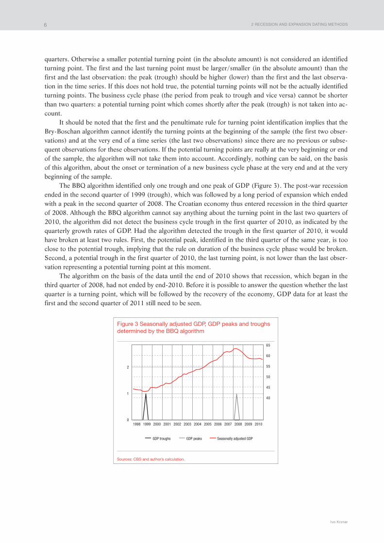
Figure 3 Seasonally adjusted GDP, GDP peaks and troughs determined by the BBQ algorithm


1998 1999 2000 2001 2002 2003 2004 2005 2006 2007 2008 2009 2010

GDP troughs GDP peaks Seasonally adjusted GDP

quarters. Otherwise a smaller potential turning point (in the absolute amount) is not considered an identified turning point. The first and the last turning point must be larger/smaller (in the absolute amount) than the first and the last observation: the peak (trough) should be higher (lower) than the first and the last observa-tion in the time series. If this does not hold true, the potential turning points will not be the actually identified turning points. The business cycle phase (the period from peak to trough and vice versa) cannot be shorter than two quarters: a potential turning point which comes shortly after the peak (trough) is not taken into ac-count.

It should be noted that the first and the penultimate rule for turning point identification implies that the Bry-Boschan algorithm cannot identify the turning points at the beginning of the sample (the first two obser-vations) and at the very end of a time series (the last two observations) since there are no previous or subse-quent observations for these observations. If the potential turning points are really at the very beginning or end of the sample, the algorithm will not take them into account. Accordingly, nothing can be said, on the basis of this algorithm, about the onset or termination of a new business cycle phase at the very end and at the very beginning of the sample.

The BBQ algorithm identified only one trough and one peak of GDP (Figure 3). The post-war recession ended in the second quarter of 1999 (trough), which was followed by a long period of expansion which ended with a peak in the second quarter of 2008. The Croatian economy thus entered recession in the third quarter of 2008. Although the BBQ algorithm cannot say anything about the turning point in the last two quarters of 2010, the algorithm did not detect the business cycle trough in the first quarter of 2010, as indicated by the quarterly growth rates of GDP. Had the algorithm detected the trough in the first quarter of 2010, it would have broken at least two rules. First, the potential peak, identified in the third quarter of the same year, is too close to the potential trough, implying that the rule on duration of the business cycle phase would be broken. Second, a potential trough in the first quarter of 2010, the last turning point, is not lower than the last obser-vation representing a potential turning point at this moment.

The algorithm on the basis of the data until the end of 2010 shows that recession, which began in the third quarter of 2008, had not ended by end-2010. Before it is possible to answer the question whether the last quarter is a turning point, which will be followed by the recovery of the economy, GDP data for at least the first and the second quarter of 2011 still need to be seen.



7

2.3 Ma rkov regime switching model

Any definition of a business cycle puts an emphasis on regime switches, i.e. changes in the state of the business cycle. The Markov regime switching model, which endogenously estimates the date of a regime switch in model parameters, is thus a useful tool for modelling the two states of business cycles. In contrast to a non-parametric method of identifying the turning points, the parametric approach assumes a data generating pro-cess the parameters of which should be estimated. This model is popular as a method for detecting the turning points (of any variable) due to its simplicity, transparency and possibility of reproduction (in contrast to mod-els that involve a subjective view of the turning points, such as the NBER analysis). In addition, many studies dating the periods of recession and expansion propose this model as a much faster and more precise method of turning point determination than other methods (e.g. see Chauvet and Piger, 2003, Chauvet and Hamilton, 2005 and Bengoechea, Camacho and Pérez-Quirós, 2004 for the EU).

In this paper we use the simple Markov regime switching model as in Hamilton (1989). The model can be simply estimated and can be used for analysis and prediction of the state of the business cycle on the ba-sis of movements of the quarterly growth rate . Hamilton’s idea is based on the fact that the expected value of the GDP growth rate (or any other variable that is an economic activity indicator) is different in the recession phase than in the expansion phase

( )E yt 1n= if economy is in expansion ( )E yt 2n= if economy is in recession (2)

with >1 2n n , or

( )E yt stn= (3)

,s 1 2tn n n= " , where ,s 0 1t = " , is an unobserved regime variable, i.e. state of the business cycle variable. Natu-rally, the economic activity model arising from Hamilton’s idea

y et s ttn= + (4)

is not sufficient to explain the GDP growth rate dynamics. If there is autocorrelation, it is hidden in the error. Assuming that the error is a process AR(1)

e e ut t t1t= +- (5)

its substitution in (4) will produce the final GDP growth rate model which should be estimated

( )y y ut s t s t1t t 1n t n= + - +- -

(0, )u IINt2+ v (6)

where it is assumed that the variance for the GDP growth rate (model error) does not change in the two re-gimes.

The quarterly growth rate in the model yt, depends on an unobserved variable st, representing the state of the business cycle. Naturally, if the state of the business cycle st were the observed variable, that model would simply be estimated using a binary variable. Hamilton (1989) shows that the above model, regardless of the fact that the regime variable is an unobserved variable, can be estimated by applying additional restrictions to the probability process that stands behind the regime switch. In the present paper, as in Hamilton (1989), it is assumed that the probability process is the first order Markov chain: any information set X about the current regime is contained in the value of the state in the previous period. Accordingly, the transition probabilities of a change of state from state i to state j, pij have the following property:


Ivo Krznar

8

10 See discussion in Bengoechea, Camacho and Pérez-Quirós (2004) about the details of poor specification of turning points in estimating the model: y y ut s t t1tn t= + +- , which actually has two states of the business cycle ( ,s 0 1*

t = " ,).

( , ) ( )Pr Prs j s i s j s i pt t t t t ij1 1 1X= = = = = =- - - (7)

Although we refer to two states of economic activity, Hamilton (1994) shows that in the case of process AR(1) for the GDP growth rate there are four “states” of the economic activity s*t ={1, 2, 3, 4}

( )y y ut t t1 1 1n t n= + - +- if economy in t and t – 1 is in expansion ( )y y ut t t1 1 0n t n= + - +- if economy in t is in expansion, and in t – 1 in recession ( )y y ut t t0 1 1n t n= + - +- if economy in t is in recession, and in t – 1 in expansion ( )y y ut t t0 1 0n t n= + - +- if economy in t and t – 1 is in recession (8)

In other words, although there are two constants in the model whose values depend on the state of eco-nomic activity, there are in reality four different constant values in four different states of the business cycle, which are functions of 0n and 1n . The turning points would not be adequately specified without the four states of economic activity defined in such a manner.10 For four states of the business cycle and the total probability theorem, the process for the conditional probability vector of each state is given as:

( 1)

( )

( )

( )

( 1)

( )

( )

( )

Pr

Pr

Pr

Pr

Pr

Pr

Pr

Pr

ssss

pppp

pppp

pppp

pppp

ssss

234

234

*

*

*

*

*

*

*

*

t

t

t

t

t

t

t

t

1

1

1

1

11

12

13

14

21

22

23

24

31

32

33

34

41

42

43

44

=

=

=

=

=

=

=

=

=

+

+

+

+

J

L

KKKKK

J

L

KKKKK

J

L

KKKKK

N

P

OOOOO

N

P

OOOOO

N

P

OOOOO

(9)

where pij denotes a transition probability of a shift of economy from state j to state i. Every probability pij is one of the model parameters that should be estimated. Since it is not possible for the economy, for instance, to jump from state 1 to state 4, the restrictions on the transition probability matrix will reduce the number of pa-rameters to be estimated. If transition probabilities are written in the following manner:

( )Pr s s p1 1t t 1= = =- ( 1)Pr s s p0 1t t 1= = = -- ( )Pr s s q0 0t t 1= = =- ( )Pr s s q1 0 1t t 1= = = -- (10)

the conditional probabilities with normal restrictions become

( )

( )

( )

( )

( )

( )

( )

( )

Pr

Pr

Pr

Pr

Pr

Pr

Pr

Pr

ssss

pp

qq

pp

qq

ssss

1234

100

00

1100

00

1

1234

*

*

*

*

*

*

*

*

t

t

t

t

t

t

t

t

1

1

1

1

=

=

=

=

=-

-

-

-

=

=

=

=

+

+

+

+

J

L

KKKKK

J

L

KKKKK

J

L

KKKKK

N

P

OOOOO

N

P

OOOOO

N

P

OOOOO

(11)

meaning that instead of 16 parameters of the transition probability matrix we need to estimate only two param-eters: p, i.e. the probability that we are in expansion after having been in expansion in the previous period and q, i.e. the probability that we are in recession after having been in recession in the previous period. These two parameters are also indicative of the persistence of recession and expansion.

In addition to the parameters of transition probabilities p i q, describing the probability process under-lying the change in the state of the economy, we also need to estimate the remaining model parameters (6): autoregressive coefficient t , the constant in the two regimes stn and error variance 2v . All the previously men-tioned parameters are calculated (estimated) by using a numerical BFGS method for maximising a conditional log likelihood function ( )ln f yt t 1X -6 @ by parameters to be estimated

( )lnl f yt t tt

T

11

X= -

=

6 @/ (12)



9

By applying the total probability theorem, conditional density can be broken down into four components (since there are actually four states of economic activity) as weighted sum of densities, conditioned on the state, where the weights are state probabilities

( ) ( , ) ( )Prf y f y s i s i* *t t t t t t t

i1 1 1

1

4

X X X= = =- - -

=

/ (13)

Since errors ut are assumed to be normally distributed, the GDP growth rate yt is also normally distrib-uted with the expectation and variance being the function of expectation and variance of the error.11

( , )f y s i e21*

( )

t t t

y y

1 2t s t s

21

2t t 1

rvX= = v

n t n

--

- - -- -^ h

(14)

For the final formulation of the log likelihood function we must calculate the individual state probabilities ( )Pr s i*t t 1X - . By applying the total probability theorem, conditional state probabilities can again be calculated

recursively

( ) ( , ) ( )Pr Pr Prs i s i s j s j* * * *t t t t t t t

i1 1 1 1 1

1

4

X X X= = = = =- - - - -

=

/ (15)

where, for example, ( , ) ( )Pr Prs s s s p1 1 1 1* * * *t t t t t1 1 1X= = = = = =- - - , and ( )Pr s j*

t t1 1X=- - can be expressed in the following manner by applying the Bayes’ theorem

( ) ( , )( , ) ( )

( , ) ( )Pr Pr

Pr

Prs j s j y

f y s i s i

f y s j s j* *

1* *

1* *

t t t t t

t t t t ti

t t t t t1 1 1 1 2

1 2 1 21

41 2 1 2X X

X X

X X= = = =

= =

= =- - - - -

- - - - -

=

- - - - -

/ (16)

It should be noted that ( )Pr s i*t t 1X= - is a function of ( )Pr s i*

t t1 2X=- - . Therefore, the equations (15) and (16) may be iterated forward in the algorithm as in the Kalman filter (for details see Hamilton, 1994) in order to recursively derive conditional probabilities ( )Pr s*t t 1X - . After that log likelihood can be written as a function of unknown parameters and the initial state of economic activity in the original period and unknown parameters can be numerically found maximising that function as ML estimators for model parameters.

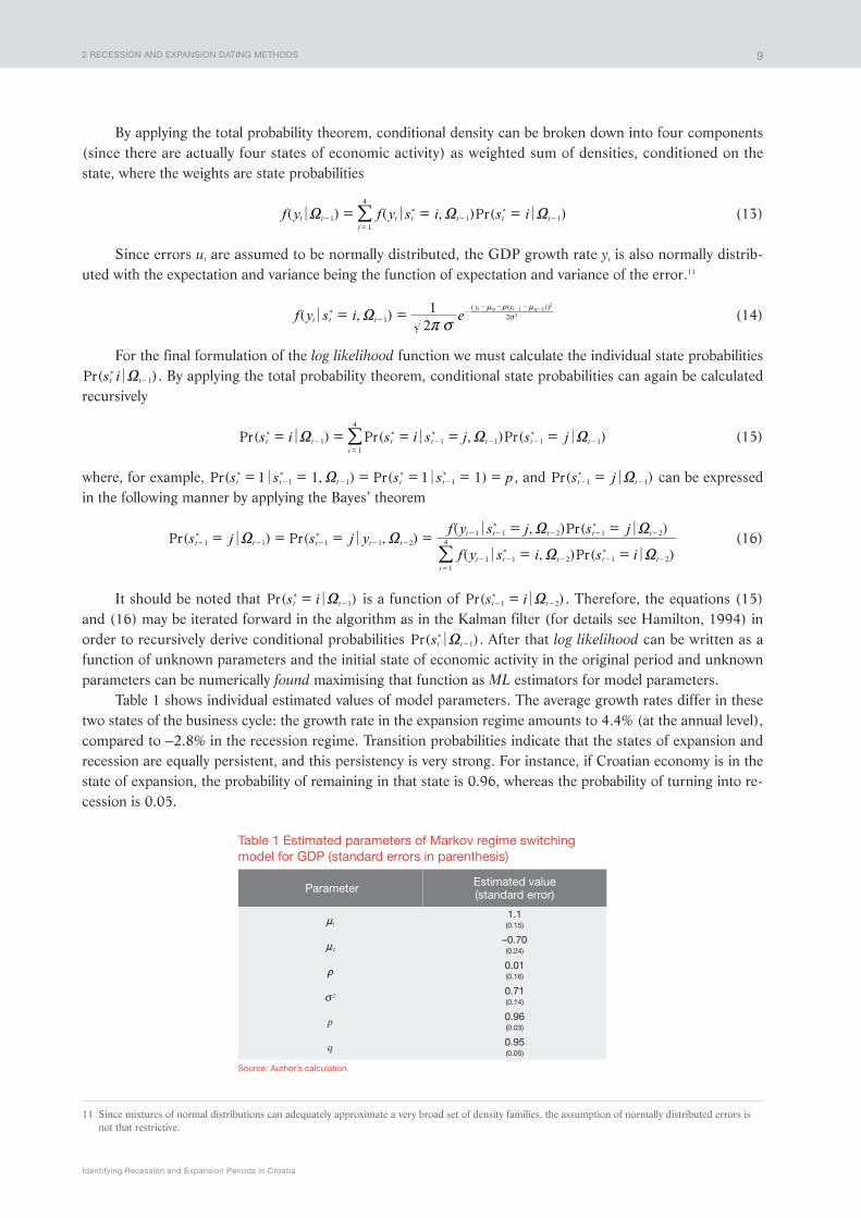
Table 1 shows individual estimated values of model parameters. The average growth rates differ in these two states of the business cycle: the growth rate in the expansion regime amounts to 4.4% (at the annual level), compared to –2.8% in the recession regime. Transition probabilities indicate that the states of expansion and recession are equally persistent, and this persistency is very strong. For instance, if Croatian economy is in the state of expansion, the probability of remaining in that state is 0.96, whereas the probability of turning into re-cession is 0.05.

11 Since mixtures of normal distributions can adequately approximate a very broad set of density families, the assumption of normally distributed errors is not that restrictive.

Table 1 Estimated parameters of Markov regime switching model for GDP (standard errors in parenthesis)

Parameter Estimated value(standard error)

1n1.1(0.15)

2n–0.70(0.24)

t0.01(0.16)

2v0.71(0.14)

p 0.96(0.03)

q 0.95(0.05)

Source: Author’s calculation.


Ivo Krznar

10

40

45

50

55

60

65

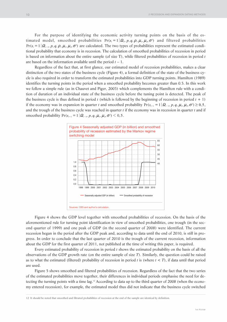
Figure 4 Seasonally adjusted GDP (in billion) and smoothed probability of recession estimated by the Markov regime switching model


1998 1999 2000 2001 2002 2003 2004 2005 2006 2007 2008 2009 2010

Seasonally adjusted GDP (in billion) Smoothed probability of recession

0.0

0.2

0.4

0.6

0.8

1.0

For the purpose of identifying the economic activity turning points on the basis of the es-timated model, smoothed probabilities ( , , , , , , )Pr s p q1t T 1 2

2t n n vX= and filtered probabilities ( , , , , , , )Pr s p q1t t 1 1 2

2t n n vX= - are calculated. The two types of probabilities represent the estimated condi-tional probability that economy is in recession. The calculation of smoothed probabilities of recession in period is based on information about the entire sample (of size T), while filtered probabilities of recession in period t are based on the information available until the period t – 1.

Regardless of the fact that, at first glance, our estimated model of recession probabilities, makes a clear distinction of the two states of the business cycle (Figure 4), a formal definition of the state of the business cy-cle is also required in order to transform the estimated probabilities into GDP turning points. Hamilton (1989) identifies the turning points in the period when a smoothed probability becomes greater than 0.5. In this work we follow a simple rule (as in Chauvet and Piger, 2003) which complements the Hamilton rule with a condi-tion of duration of an individual state of the business cycle before the tuning point is detected. The peak of the business cycle is thus defined in period t (which is followed by the beginning of recession in period t + 1) if the economy was in expansion in quarter t and smoothed probability ( , , , , , ) ,Pr s p q1 0 5t t1 1 1 2

2 $n n vX=+ - , and the trough of the business cycle was reached in quarter t if the economy was in recession in quarter t and if smoothed probability ( , , , , , ) 0,5Pr s p q1t t1 1 1 2

2 1n n vX=+ - .

Figure 4 shows the GDP level together with smoothed probabilities of recession. On the basis of the aforementioned rule for turning point identification in view of smoothed probabilities, one trough (in the sec-ond quarter of 1999) and one peak of GDP (in the second quarter of 2008) were identified. The current recession began in the period after the GDP peak and, according to data until the end of 2010, is still in pro-gress. In order to conclude that the last quarter of 2010 is the trough of the current recession, information about the GDP for the first quarter of 2011, not published at the time of writing this paper, is required.

Every estimated probability of recession in period t shows the estimated probability on the basis of all the observations of the GDP growth rate (on the entire sample of size T). Similarly, the question could be raised as to what the estimated (filtered) probability of recession in period t is (where t < T), if data until that period are used.

Figure 5 shows smoothed and filtered probabilities of recession. Regardless of the fact that the two series of the estimated probabilities move together, their differences in individual periods emphasise the need for de-tecting the turning points with a time lag.12 According to data up to the third quarter of 2008 (when the econo-my entered recession), for example, the estimated model thus did not indicate that the business cycle switched

12 It should be noted that smoothed and filtrated probabilities of recession at the end of the sample are identical by definition.

3 ROBUSTNESS ANALYSIS: A DYNAMIC FACTOR


11

Figure 5 Smoothed and filtered probability of recession estimated by the Markov regime switching model


1998 1999 2000 2001 2002 2003 2004 2005 2006 2007 2008 2009 2010

Smoothed probability of recession Filtered probability of recession

0.0

0.2

0.4

0.6

0.8

1.0

from the state of expansion to the state of recession. Furthermore, according to data up to the third quarter of 2010, the estimated model points to a considerable decrease in probability that the Croatian economy is in re-cession. On the other hand, smoothed probabilities, which also take into account the information about GDP in the fourth quarter of 2010, show that the Croatian economy was still in recession at the end of 2010.

3 Robustness analysis: a dynamic factor

In analysing detection of turning points, we used the quarterly GDP growth rate as a relevant and single indicator of economic activity dynamics. Recessions and expansions are caused by different shocks affecting different variables (which in turn affect GDP). Therefore, inclusion of many different variables increases the model’s precision in distinguishing the periods of recession from the periods of expansion. In addition, a mix-ture of variables in the model may reduce errors in measuring individual series, thus decreasing the probability of incorrectly identified turning points. Furthermore, many definitions of the state of the business cycle place an emphasis on the importance of co-movements of a large number of relevant variables describing economic activity. NBER’s business cycle analysis, as the fundamental method of turning point identification is based not only on GDP movements, but also on variables such as employment and industrial production.

There are two approaches to the state of the business cycle analysis on the basis of a large number of vari-ables. It is possible to use individual time series for which individual turning points are detected (whether by means of Bry-Boschan algorithm or the Markov regime switching model), which are then consolidated in the common turning points (see the algorithm in Harding and Pagan, 2002) or all the information on the basis of an identical set of individual variables can be used in order to estimate the common factor that best approxi-mates movements of variables used in its estimation. In this work, a dynamic factor model is estimated as in Stock and Watson (1991) on the basis of 11 time series which are considered to describe, to the largest extent, the economic activity in Croatia. One of these variables is the GDP growth rate. The results of the estimated factor will not change significantly if GDP is eliminated from the set of 11 variables. On the basis of move-ments of the factor as an economic activity indicator, the periods of recession and the periods of expansion will be identified in the same manner as in the use of a quarterly GDP growth rate and the Bry-Boschan algorithm and the estimation of the Markov regime switching model.

Literature on dynamic factor model begins with Geweke’s theoretical work (1977) and an empirical


Ivo Krznar

12

application of the model in Sargent and Sims (1977).13 The dynamic factor model is today very popular in view of the possibility of modelling a large number of time series (exceeding the number of observations). The key idea of the dynamic factor model is that several unobserved dynamic factors fit stand behind the co-movements of a large number of macroeconomic variables Xt that are stationary. The main conclusion of the empirical research (see for instance Giannone, Reichlin and Sala, 2004 or Watson, 2004) on dynamic factors for the American economy is that a small number of factors (only two) explains a very large proportion of vari-ation of many macroeconomic variables. Apart from the fact that every variable is affected by the movements of the common factors, their movement is also under the influence of idiosyncratic errors eit, which are a conse-quence of measurement errors or specific shocks. Unobserved factors, as well as model errors, are modelled as a stochastic process, commonly assumed to be vector autoregressive (VAR) process. Accordingly, the dynamic factor model (Stock and Watson, 1991) is written as:

( )X L f et t tm= + ( )L ft thW = ( )L et tyC = (17)

where ...e e e et t t t1 2 11= l6 @ ...t t t t1 2 11y y y y= l6 @

,NID00 0

0t

t

2

+hy

vW

he e eeo o oo

while L is a lag operator (e.g. L f fpt t p= - ), lag polynomial ( )Lim is referred to as a dynamic factor loading for

the i-th series, ( )L fi tm is a common component for the i-th series. The idiosyncratic errors are assumed to be uncorrelated with each other at all forward and backward lags. The matrix W represents a covariance matrix of the error vector ty .

For the purpose of model simplicity, it is assumed that only one factor is behind the co-movement of the 11 indicated macrovariables.14 Errors et, as well as the common factor follow the AR(1) process:

( ) ( )L L1i i1cC = - ; ( ) ( )L L1 f{W = - . The relationship between the common factor and the macrovariables is coincidental: ( )Lm m= .

This model, under the above assumptions, may be written in the state space form (commonly referred to as the dynamic factor model in static form) as an observable equation

X HZt t= (18)

and a state equation with a state vector Zt

Z Zt t t1b g= +- (19)

where(0, )NID Qt +g

...t t t t t1 2 11g h y y y= l6 @

... ... ... ... ...

Q00

0

0

0

0

00

0

000

0

000

2

12

22

112

vv

v

v

=

h

R

T

SSSSSSS

V

X

WWWWWWW

13 For an overview of the key theoretical results, application and conclusions in literature about dynamic factor models see Stock and Watson (2010).

14 For more information about the testing of the number of factors see Bai and Ng (2002).



13

and

...Z f e e et t t t t1 2 11= l6 @

... ... ... ...

...

...

...

...

...

...

H

100

0

010

0

001

0

000

1

1

2

3

11

mmm

m

=

R

T

SSSSSSS

V

X

WWWWWWW

, ... ... ... ... ...

00

0

0

0

0

00

0

000

0

000

f

1

2

11

b

{c

c

c

=

R

T

SSSSSSS

V

X

WWWWWWW

Once the model is written in the state space form, its parameters, including the factor values ft, can be es-timated by a maximum likelihood method and Kalman filter on the basis of which the log likelihood function is calculated (assuming normally distributed errors).15

Note that the only observed variables in that model are the vector Xt variables. Factor values and error val-ues (placed in the vector Zt) are unobserved. That is the reason for using the Kalman filter in calculating likeli-hood, on the basis of which the model parameters will be estimated, for the calculation of values of unobserved variables in a manner described below. If estimation Zt is denoted by Zt x on the basis of all the information until the period x and its covariance matrix is denoted by Pt x , the prediction equations are the following

Z Zt t t t1 1 1b=- - - (20)

P P Qt t t t1 1 1b b= +- - - l (21)

These equations are used to calculate the prediction errors

X HZt t t t t1 1s = -- - (22)

and the covariance matrix

R HP Ht t t t1 1=- - l (23)

Accordingly, log likelihood function in every algorithm iteration is written as

( )lnl R R21 2 2

1t t t t t t t t t1 1 1

11r s s=- -- - -

--l^ h (24)

Finally, the state vector and its covariance matrix are updated on the basis of the following formulas:

Z Z Kt t t t t t t1 1 1 1s= ++ + - - (25)

P P K HPt t t t t t t1 1= -- - (26)

where ( )K P H Rt t t t t1 11= - -

-l is a Kalman gain. The initial values Z0 0 and P0 0 with which the algorithm is started equal the zero vector and a unit matrix respectively.

Most of the data used in the estimation of factors and dynamic factor model parameters are published by the Central Bureau of Statistics. All the data, apart from those on domestic GDP, are published on a monthly basis. Monthly data are quarterly averaged and then adjusted for seasonal and calendar effect (except for the prices of foreign borrowing, loans and producer price index). The time series of employment (Z) relates to the number of those employed in legal persons. Exports (X) and imports (IM) represent the nominal value of goods and services. Trade turnover index (TTM) and index of industrial production (IND) relate to aggregate indices of the same variables. PPI is an overall producer price index. The series BDP represents the Croatian

15 For details of the Kalman filter derivation see Hamilton (1994).


Ivo Krznar

14

–3

–2

–1

0

1

2

3

4

Figure 6 Quarterly GDP growth rates and common component estimated by the factor model


1998 1999 2000 2001 2002 2003 2004 2005 2006 2007 2008 2009 2010

Common component Quarterly GDP growth rate

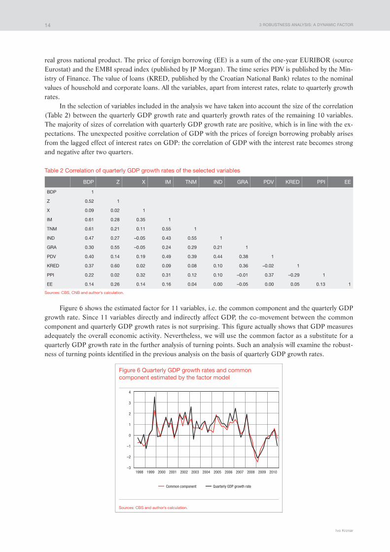
real gross national product. The price of foreign borrowing (EE) is a sum of the one-year EURIBOR (source Eurostat) and the EMBI spread index (published by JP Morgan). The time series PDV is published by the Min-istry of Finance. The value of loans (KRED, published by the Croatian National Bank) relates to the nominal values of household and corporate loans. All the variables, apart from interest rates, relate to quarterly growth rates.

In the selection of variables included in the analysis we have taken into account the size of the correlation (Table 2) between the quarterly GDP growth rate and quarterly growth rates of the remaining 10 variables. The majority of sizes of correlation with quarterly GDP growth rate are positive, which is in line with the ex-pectations. The unexpected positive correlation of GDP with the prices of foreign borrowing probably arises from the lagged effect of interest rates on GDP: the correlation of GDP with the interest rate becomes strong and negative after two quarters.

Table 2 Correlation of quarterly GDP growth rates of the selected variables

BDP Z X IM TNM IND GRA PDV KRED PPI EE

BDP 1

Z 0.52 1

X 0.09 0.02 1

IM 0.61 0.28 0.35 1

TNM 0.61 0.21 0.11 0.55 1

IND 0.47 0.27 –0.05 0.43 0.55 1

GRA 0.30 0.55 –0.05 0.24 0.29 0.21 1

PDV 0.40 0.14 0.19 0.49 0.39 0.44 0.38 1

KRED 0.37 0.60 0.02 0.09 0.08 0.10 0.36 –0.02 1

PPI 0.22 0.02 0.32 0.31 0.12 0.10 –0.01 0.37 –0.29 1

EE 0.14 0.26 0.14 0.16 0.04 0.00 –0.05 0.00 0.05 0.13 1

Sources: CBS, CNB and author’s calculation.

Figure 6 shows the estimated factor for 11 variables, i.e. the common component and the quarterly GDP growth rate. Since 11 variables directly and indirectly affect GDP, the co-movement between the common component and quarterly GDP growth rates is not surprising. This figure actually shows that GDP measures adequately the overall economic activity. Nevertheless, we will use the common factor as a substitute for a quarterly GDP growth rate in the further analysis of turning points. Such an analysis will examine the robust-ness of turning points identified in the previous analysis on the basis of quarterly GDP growth rates.



15

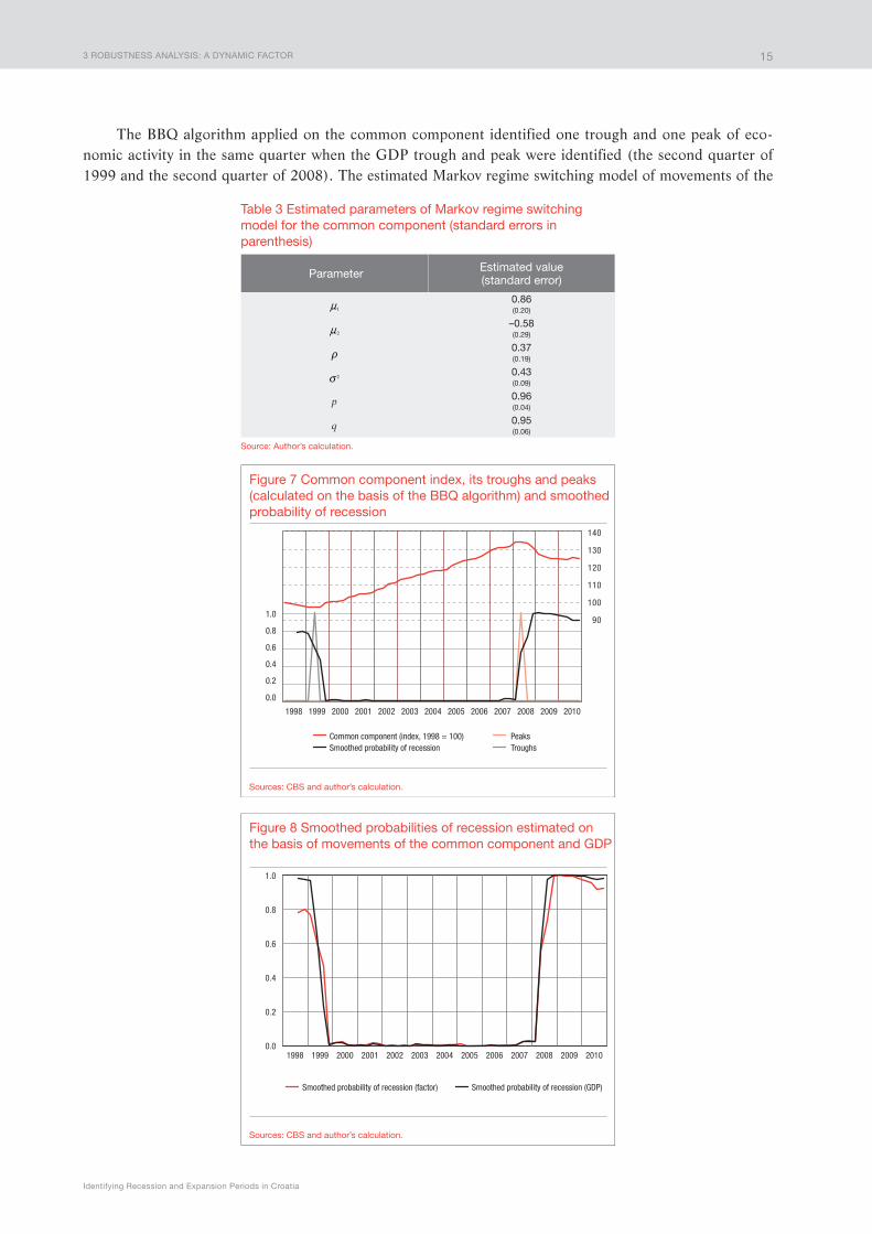
Table 3 Estimated parameters of Markov regime switching model for the common component (standard errors in parenthesis)

Parameter Estimated value(standard error)

1n0.86(0.20)

2n–0.58(0.29)

t0.37(0.19)

2v0.43(0.09)

p 0.96(0.04)

q 0.95(0.06)

Source: Author’s calculation.

The BBQ algorithm applied on the common component identified one trough and one peak of eco-nomic activity in the same quarter when the GDP trough and peak were identified (the second quarter of 1999 and the second quarter of 2008). The estimated Markov regime switching model of movements of the

90

100

110

120

130

140

Figure 7 Common component index, its troughs and peaks (calculated on the basis of the BBQ algorithm) and smoothed probability of recession


1998 1999 2000 2001 2002 2003 2004 2005 2006 2007 2008 2009 2010

Common component (index, 1998 = 100) PeaksTroughsSmoothed probability of recession

0.0

0.2

0.4

0.6

0.8

1.0

Figure 8 Smoothed probabilities of recession estimated on the basis of movements of the common component and GDP


1998 1999 2000 2001 2002 2003 2004 2005 2006 2007 2008 2009 2010

Smoothed probability of recession (factor) Smoothed probability of recession (GDP)

0.0

0.2

0.4

0.6

0.8

1.0

4 CONCLUSION

Ivo Krznar

16

common component (Table 3), estimated smoothed probabilities and the rule applied in determining GDP turning points identify the same periods as turning points of the Croatian economic activity. Figure 7 shows the common component index (1st quarter 1998 = 100), the trough and peak detected by the BBQ algorithm and smoothed probabilities estimated by the Markov regime switching model.

Figure 8 compares smoothed probabilities of recession estimated by the Markov switching model for the GDP growth rate and for the common component. Compared to the probability of recession estimated on the basis of GDP data, which remained at a high level until the end of 2010, probability of recession estimated us-ing factor data fell from mid 2009 to the end of 2010 (nevertheless, that probability was still above 0.5). Such a reduction in probability of recession may be a consequence of a strong export growth, recovery of lending activity focused on corporates and households and a considerable decline in prices of borrowing on the foreign market from mid 2009. Movements of these variables probably contributed most to a slight fall in the factor index during 2009 and at end-2010.

3.1 Comparison of the identified turning points

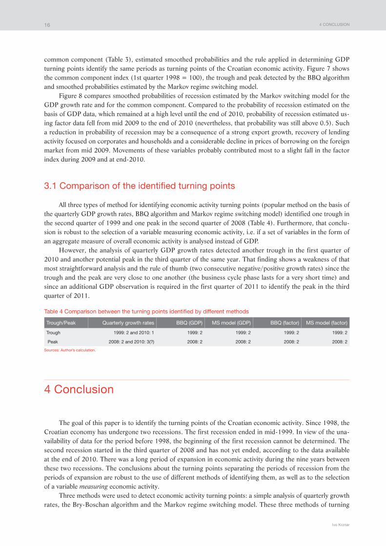
All three types of method for identifying economic activity turning points (popular method on the basis of the quarterly GDP growth rates, BBQ algorithm and Markov regime switching model) identified one trough in the second quarter of 1999 and one peak in the second quarter of 2008 (Table 4). Furthermore, that conclu-sion is robust to the selection of a variable measuring economic activity, i.e. if a set of variables in the form of an aggregate measure of overall economic activity is analysed instead of GDP.

However, the analysis of quarterly GDP growth rates detected another trough in the first quarter of 2010 and another potential peak in the third quarter of the same year. That finding shows a weakness of that most straightforward analysis and the rule of thumb (two consecutive negative/positive growth rates) since the trough and the peak are very close to one another (the business cycle phase lasts for a very short time) and since an additional GDP observation is required in the first quarter of 2011 to identify the peak in the third quarter of 2011.

Table 4 Comparison between the turning points identified by different methods

Trough/Peak Quarterly growth rates BBQ (GDP) MS model (GDP) BBQ (factor) MS model (factor)

Trough 1999: 2 and 2010: 1 1999: 2 1999: 2 1999: 2 1999: 2

Peak 2008: 2 and 2010: 3(?) 2008: 2 2008: 2 2008: 2 2008: 2

Sources: Author’s calculation.

4 Conclusion

The goal of this paper is to identify the turning points of the Croatian economic activity. Since 1998, the Croatian economy has undergone two recessions. The first recession ended in mid-1999. In view of the una-vailability of data for the period before 1998, the beginning of the first recession cannot be determined. The second recession started in the third quarter of 2008 and has not yet ended, according to the data available at the end of 2010. There was a long period of expansion in economic activity during the nine years between these two recessions. The conclusions about the turning points separating the periods of recession from the periods of expansion are robust to the use of different methods of identifying them, as well as to the selection of a variable measuring economic activity.

Three methods were used to detect economic activity turning points: a simple analysis of quarterly growth rates, the Bry-Boschan algorithm and the Markov regime switching model. These three methods of turning

REFERENCES


17

point detection identified one trough in the second quarter of 1999. Although the simplest analysis of quarterly GDP growth rates detected a GDP peak in the second quarter of 2008, followed by the entry of the Croatian economy into recession, the same analysis cannot explain the state of the business cycle in 2010. This problem points to the traps that must be borne in mind in the analysis of the state of economic activity by that popular method. On the other hand, the Bry-Boschan algorithm and the estimated Markov regime switching model identified one peak of economic activity in the second quarter of 2008, clearly indicating that the Croatian economy has, from that point on, been in a recession that is still in progress, according to the data at the end of 2010. The conclusion on whether the GDP trough was reached in the last quarter requires a minimum of two GDP observations in 2011 for the Bry-Boschan algorithm, or only one GDP observation in the first quarter of 2011 for the Markov switching model.

The Bry-Boschan algorithm and Markov regime switching model represent a significant advance in the analysis of the business cycle in Croatia: two methods that are transparent in determining the state of econom-ic activity and whose results can easily be reproduced are publicly available. Furthermore, since the estimation of the factor model uses data that are generally published somewhat earlier than GDP data, the Markov regime switching model with its capability for estimating recession probability can analyse the state of the business cycle before the first publication of the GDP data. However, a prompt estimation of economic dynamics and identification of the new turning point in real time are left for future research. The models developed by Čeh and Kunovac (2009), based on the estimation of the static factor of the Croatian economy on a monthly ba-sis, represent a step forward in that direction. In addition, the Markov regime switching model with a dynamic factor estimated on the basis of monthly data could also improve the methodology, the objective of which is to analyse the state of economic activity in real time.

References

Ahec-Šonje, A. (ed.) (1996): Navješćujući indikatori hrvatskog gospodarstva, Osnovna studija, Ekonomski in-stitut, Zagreb, Zagreb.

Artis, M. (2002): Dating the Business Cycle in Britain, University of Manchester, CGBCR, Discussion Paper 017.

Artis, M., and W. Zhang (1999): Further evidence on the international business cycle and the ERM: is there a European business cycle?, Oxford Economic Papers, 51, pp. 120-132.

Bačić, K. (ed.) (2004): Usavršavanje prognostičkog indeksa hrvatskog gospodarstva, Završna studija, Ekonom-ski institut, Zagreb, Zagreb.

Bai, J., and S. Ng (2002): Determining the Number of Factors in Approximate Factor Models, Econometrica, Econometric Society, vol. 70(1), pp. 191-221.

Bengoechea, P., M. Camacho, and G. Pérez-Quirós (2004): A Useful Tool to Identify Recessions in the Euro-area, European Commission, Directorate-General for Economic and Financial Affairs, Economic Paper 215.

Boehm, E. A., and G. H. Moore (1984): New Economic Indicators for Australia, 1949-84, Australian Eco-nomic Review, 4th Quarter, pp. 34-56.

Bry, G., and C. Boschan (1971): Cyclical Analysis of Time Series: Selected Procedures and Computer Programs, New York: National Bureau of Economic Research.

REFERENCES

Ivo Krznar

18

Cerovac, S. (2005): Novi kompozitni indikatori za hrvatsko gospodarstvo: prilog razvoju domaćeg sustava cikličkih indikatora, Istraživanja HNB-a, No. 16, April 2005.

Chauvet, M., and J. D. Hamilton (2005): Dating Business Cycle Turning Points, NBER, Working Paper 11422.

Chauvet, M., and J. Piger (2003): Identifying Business Cycle Turning Points in Real Time, Federal Reserve Bank of St. Louis Review 85, pp. 47-61.

Chauvet, M., and J. M. Piger (2007): A Comparison of the Real-Time Performance of Business Cycle Dating Methods, not published.

Christoffersen, P. F. (2000): Dating the Turning Points of Nordic Business Cycles, University of Copenhagen, Department of Economics, EPRU, Working Paper 13.

Čeh, A. M., and D. Kunovac (2009): Brza procjena BDP-a korištenjem velikog broja mjesečnih indikatora, Cro-atian National Bank, in manuscript.

Geweke, J. (1977): The Dynamic Factor Analysis of Economic Time Series, in Latent Variables in Socio-Eco-nomic Models, D. J. Aigner and A. S. Goldberger (ed.), Amsterdam, North-Holland.

Giannone, D., L. Reichlin, and L. Sala (2004): Monetary Policy in Real Time, NBER Macroeconomics Annual, pp. 161-200.

Hamilton, J. D. (1989): A New Approach to the Economic Analysis of Nonstationary Time Series and the Busi-ness Cycle. Econometrica, March 57(2), pp. 357-384.

Hamilton, J. D. (1994): Time Series Analysis, Princeton University.

Harding, D. (1997): The Definition, Dating and Duration of Cycles, University Library of Munich, MPRA Pa-per 3357.

Harding, D. (2003): Towards an Econometric Foundation for Turning Point Based Analysis of Dynamic Pro-cesses, Paper presented at the 2003 Australian Meeting of the Econometric Society.

Harding, D., and A. Pagan (2001): Extracting, Using and Analysing Cyclical Information, University Library of Munich, MPRA Paper 15.

Harding, D., and A. Pagan (2002): Dissecting the Cycle: A Methodological investigation, Journal of Monetary Economics, 49, pp. 365-381.

Harding, D., and A. Pagan (2003): A Comparison of two Business Cycle Dating Methods, Journal of Economic Dynamics and Control, 27, pp. 1681-1690.

Krolzig, H.-M. (2001): Markov-Switching Procedures for Dating the Euro-Zone Business Cycle, Vierteljahres-hefte zur Wirtschaftsforschung, 70(3), pp. 339-351.

Krolzig, H.-M., and J. Toro (2005): Classical and Modern Business Cycle Measurement: The European Case, Spanish Economic Review, 7, pp. 1-21.

Mitchell, J., and K. Mouratidis (2002): Is there a common Euro-zone business cycle?, Paper presented at the Eurostat Colloquium on Modern tools for Business Cycle Analysis, Luxembourg, 28-29 November 2002.

REFERENCES


19

Morley, J., and J. Piger (2005): The Importance of Nonlinearity in Reproducing Business Cycle Features, The Federal Reserve Bank of St. Louis, Working Paper 032B.

Sargent, T. J., and C. A. Sims (1977): Business Cycle Modeling Without Pretending to Have Too Much A-Priori Economic Theory, in New Methods in Business Cycle Research, C. Sims et al. (ed.), Minneapolis, Federal Re-serve Bank of Minneapolis.

Stock, J., and M. Watson (1991): A probability model of the coincident economic indicators, in K. Lahiri and G. H. Moore (ed.), Leading Economic indicators: new approaches and forecasting records, 4th Chapter, New York, Cambridge University Press, pp. 63-85

Stock, J., and M. Watson (2011): Dynamic Factor Models, in Oxford Handbook of Forecasting, Michael P. Clements and David F. Hendry (ed.), Oxford, Oxford University Press.

Tsouma, E. (2010): Dating Business Cycle Turning Points: The Greek Economy During 1970 – 2010 and the Recent Recession, CEPR.

Watson, M. W. (2004): Comment on Giannone, Reichlin, and Sala, NBER Macroeconomics Annual, pp. 216-221.

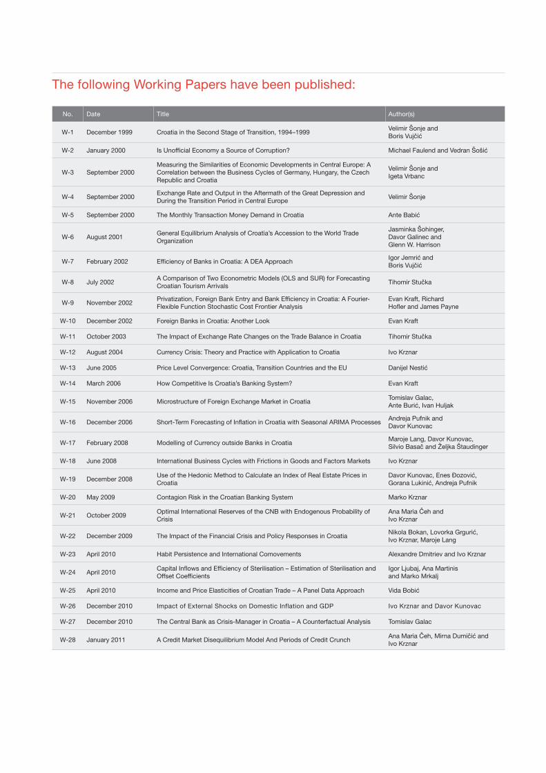
The following Working Papers have been published:

No. Date Title Author(s)

W-1 December 1999 Croatia in the Second Stage of Transition, 1994–1999Velimir Šonje andBoris Vujčić

W-2 January 2000 Is Unofficial Economy a Source of Corruption? Michael Faulend and Vedran Šošić

W-3 September 2000Measuring the Similarities of Economic Developments in Central Europe: A Correlation between the Business Cycles of Germany, Hungary, the Czech Republic and Croatia

Velimir Šonje andIgeta Vrbanc

W-4 September 2000Exchange Rate and Output in the Aftermath of the Great Depression and During the Transition Period in Central Europe

Velimir Šonje

W-5 September 2000 The Monthly Transaction Money Demand in Croatia Ante Babić

W-6 August 2001General Equilibrium Analysis of Croatia’s Accession to the World Trade Organization

Jasminka Šohinger,Davor Galinec andGlenn W. Harrison

W-7 February 2002 Efficiency of Banks in Croatia: A DEA ApproachIgor Jemrić andBoris Vujčić

W-8 July 2002A Comparison of Two Econometric Models (OLS and SUR) for Forecasting Croatian Tourism Arrivals

Tihomir Stučka

W-9 November 2002Privatization, Foreign Bank Entry and Bank Efficiency in Croatia: A Fourier-Flexible Function Stochastic Cost Frontier Analysis

Evan Kraft, RichardHofler and James Payne

W-10 December 2002 Foreign Banks in Croatia: Another Look Evan Kraft

W-11 October 2003 The Impact of Exchange Rate Changes on the Trade Balance in Croatia Tihomir Stučka

W-12 August 2004 Currency Crisis: Theory and Practice with Application to Croatia Ivo Krznar

W-13 June 2005 Price Level Convergence: Croatia, Transition Countries and the EU Danijel Nestić

W-14 March 2006 How Competitive Is Croatia’s Banking System? Evan Kraft

W-15 November 2006 Microstructure of Foreign Exchange Market in CroatiaTomislav Galac,Ante Burić, Ivan Huljak

W-16 December 2006 Short-Term Forecasting of Inflation in Croatia with Seasonal ARIMA ProcessesAndreja Pufnik andDavor Kunovac

W-17 February 2008 Modelling of Currency outside Banks in CroatiaMaroje Lang, Davor Kunovac,Silvio Basač and Željka Štaudinger

W-18 June 2008 International Business Cycles with Frictions in Goods and Factors Markets Ivo Krznar

W-19 December 2008Use of the Hedonic Method to Calculate an Index of Real Estate Prices in Croatia

Davor Kunovac, Enes Đozović,Gorana Lukinić, Andreja Pufnik

W-20 May 2009 Contagion Risk in the Croatian Banking System Marko Krznar

W-21 October 2009Optimal International Reserves of the CNB with Endogenous Probability of Crisis

Ana Maria Čeh andIvo Krznar

W-22 December 2009 The Impact of the Financial Crisis and Policy Responses in CroatiaNikola Bokan, Lovorka Grgurić,Ivo Krznar, Maroje Lang

W-23 April 2010 Habit Persistence and International Comovements Alexandre Dmitriev and Ivo Krznar

W-24 April 2010Capital Inflows and Efficiency of Sterilisation – Estimation of Sterilisation and Offset Coefficients

Igor Ljubaj, Ana Martinisand Marko Mrkalj

W-25 April 2010 Income and Price Elasticities of Croatian Trade – A Panel Data Approach Vida Bobić

W-26 December 2010 Impact of External Shocks on Domestic Inflation and GDP Ivo Krznar and Davor Kunovac

W-27 December 2010 The Central Bank as Crisis-Manager in Croatia – A Counterfactual Analysis Tomislav Galac

W-28 January 2011 A Credit Market Disequilibrium Model And Periods of Credit CrunchAna Maria Čeh, Mirna Dumičić and Ivo Krznar

Guidelines to authors

In its periodical publications Working Papers, Surveys and Technical Papers, the Croatian National Bank publishes scien-tific and scholarly papers of the Bank’s employees and other associate contributors.

After the submission, the manuscripts shall be subject to peer review and classification by the Manuscript Review and Classification Committee. The authors shall be informed of the acceptance or rejection of their manuscript for publication within two months following the manuscript submission.

Manuscripts are submitted and published in Croatian and/or English language.

Manuscripts submitted for publication should meet the fol-lowing requirements:

Manuscripts should be submitted via e-mail or optical stor-age media (CD, DVD), accompanied by one printed paper copy. The acceptable text format is Word.

The first page of the manuscript should contain the article title, first and last name of the author and his/her academic degree, name of the institution with which the author is associ-ated, author’s co-workers, and the complete mailing address of the corresponding author to whom a copy of the manuscript with requests for corrections shall be sent.

Additional information, such as acknowledgments, should be incorporated in the text at the end of the introductory section.

The second page should contain the abstract and the key words. The abstract is required to be explicit, descriptive, writ-ten in third person, consisting of not more than 250 words (maximum 1500 characters). The abstract should be followed by maximum 5 key words.

A single line spacing and A4 paper size should be used. The text must not be formatted, apart from applying bold and italic script to certain parts of the text. Titles must be numerated and separated from the text by double-line spacing, without for-matting.

Tables, figures and charts that are a constituent part of the

paper must be well laid out, containing: number, title, units of measurement, legend, data source, and footnotes. The foot-notes referring to tables, figures and charts should be indi-cated by lower-case letters (a,b,c…) placed right below. When the tables, figures and charts are subsequently submitted, it is necessary to mark the places in the text where they should be inserted. They should be numbered in the same sequence as in the text and should be referred to in accordance with that numeration. If the tables and charts were previously inserted in the text from other programs, these databases in the Excel format should also be submitted (charts must contain the cor-responding data series).

The preferred formats for illustrations are EPS or TIFF with explanations in 8 point Helvetica (Ariel, Swiss). The scanned illustration must have 300 dpi resolution for grey scale and full colour illustration, and 600 dpi for lineart (line drawings, diagrams, charts).

Formulae must be legible. Indices and superscript must be explicable. The symbols’ meaning must be given following the equation where they are used for the first time. The equations in the text referred to by the author should be marked by a se-rial number in brackets closer to the right margin.

Notes at the foot of the page (footnotes) should by indicat-ed by Arabic numerals in superscript. They should be brief and written in a smaller font than the rest of the text.

References cited in the text are listed at the last page of the manuscript in the alphabetical order, according to the authors’ last names. References should also include data on the pub-lisher, city and year of publishing.

Publishing Department maintains the right to send back for the author’s revision the accepted manuscript and illustrations that do not meet the above stated requirements.

All contributors who wish to publish their papers are wel-come to do so by addressing them to the Publishing Depart-ment, following the above stated guidelines.

The Croatian National Bank publications:

Croatian National Bank – Annual ReportRegular annual publication surveying annual monetary and general economic developments as well as statistical data.

Croatian National Bank – Semi-annual ReportRegular semi-annual publication surveying semi-annual mon-etary and general economic developments and statistical data.

Croatian National Bank – Quarterly ReportRegular quarterly publication surveying quarterly monetary and general economic developments.

Banks BulletinPublication providing survey of data on banks.

Croatian National Bank – BulletinRegular monthly publication surveying monthly monetary and general economic developments and monetary statistics.

Croatian National Bank – Working PapersOccasional publication containing shorter scientific papers written by the CNB employees and associate contributors.

Croatian National Bank – SurveysOccasional publication containing scholarly papers written by the CNB employees and associate contributors.

Croatian National Bank – Technical PapersOccasional publication containing papers of informative char-acter written by CNB employees and associate contributors.

The Croatian National Bank also issues other publications such as, for example, numismatic issues, brochures, publica-tions in other media (CD-ROM, DVD), books, monographs and papers of special interest to the CNB as well as proceed-ings of conferences organised or co-organised by the CNB, ed-ucational materials and other similar publications.

ISSN 1331-8586 (print) • ISSN 1334-0131 (online)

identifying recession and expansion periods in croatia

Documents