Identifying Preferences in Networks withBounded Degree∗

Aureo de Paula†

UCL, Sao Paulo School of Economics,

CeMMAP, IFS and CEPR

Seth Richards-Shubik‡

Lehigh University

and NBER

Elie Tamer§

Harvard University

First Version: December 2011This Version: August 2017

Abstract

This paper provides a framework for identifying preferences in a large networkwhere links are pairwise stable. Network formation models present difficulties for iden-tification, especially when links can be interdependent: e.g., when indirect connectionsmatter. We show how one can use the observed proportions of various local networkstructures to learn about the underlying preference parameters. The key assumptionfor our approach restricts individuals to have bounded degree in equilibrium, implyinga finite number of payoff-relevant local structures. Our main result provides necessaryconditions for parameters to belong to the identified set. We then develop a quadraticprogramming algorithm that can be used to construct this set. With further restrictionson preferences, we show that our conditions are also sufficient for pairwise stability andtherefore characterize the identified set precisely. Overall, the use of both the economicmodel along with pairwise stability allows us to obtain effective dimension reduction.

∗We thank seminar and conference participants at the Conference on Econometric Analysis of SocialInteractions at Northwestern University (2010), the ASSA meetings in Chicago (2012), University of WesternOntario (2013), the Stats in Paris: Statistics and Econometrics of Networks (2013) conference, the RecentAdvances in Set Identification (2013) conference, the 2nd European Meeting of Network Economics (2014),Heinz College (2015), the INET Econometrics of Networks Workshop at Cambridge University (2015), theCowles Foundation (2015), Northwestern University (2015), the Chicago Fed (2015), the Econometric SocietyWorld Congress (2015), the USC Dornsife INET Conference on Networks (2015), the New York Fed (2016),the University of Pennsylvania (2016), Surrey (2016), Groningen (2016), the Tinbergen Institute (2016),Harvard (2016), Rutgers (2016), and Virginia (2016) for suggestions and comments. We are also gratefulto A. Advani, J. Altonji, G. Chamberlain, C. Gualdani, P. Haile, T. Holden, and M. Shum for detailedcomments. de Paula gratefully acknowledges financial support from the NSF through award SES-1123990,the ERC through Starting Grant 338187, and the Economic and Social Research Council through the ESRCCentre for Microdata Methods and Practice grant RES-589-28-0001.†University College London, Sao Paulo School of Economics, CeMMAP, IFS and CEPR. E-mail:

apaula@ucl.ac.uk‡Lehigh University and NBER, E-mail: sethrs@lehigh.edu§Harvard University, E-mail: elietamer@fas.harvard.edu

1 Introduction

This paper provides a framework for studying identification—what can be learned about

parameters of interest from data—in strategic network formation models. The framework

applies to complete information games with non-transferable payoffs in which individuals,

given a particular utility function, form links with each other. Our objective is to learn

about these payoffs from observed data on network linkages. In particular, we assume that

observed networks are equilibrium networks and use pairwise stability, proposed in Jackson

and Wolinsky (1996), as the solution concept.

A network formation model founded on a well-defined preference structure for all the

players is helpful in determining how networks develop given a particular policy or incentive

system. In a variety of applications, the architecture of networks is thought to influence final

outcomes, and so it is important to understand how the networks themselves are formed.

Empirically sound network formation models can also be helpful in describing why certain

networks emerge and not others, for example tracking the effects of policies or frictions on

the kinds and shapes of networks that arise.

The problem in analyzing such strategic models is that multiplicity of solutions and other

computational difficulties are pervasive, especially when more than a handful of agents are

involved. This paper proposes a framework for studying large networks, which achieves

dimension reduction by aggregating individuals with similar network positions. We impose

restrictions on the number of links that a person would choose to have, as well as on the

cardinality of the observable characteristics. As a consequence, each individual’s position in

the network can be described as one of a finite number of possible local network structures.

This greatly reduces the dimensionality of the problem. The limitation on the number

of links, or bounded degree, is of course an important restriction. It makes this framework

appropriate for applications where individuals are observed to have a relatively small number

of connections, but not for others where it is important to have some nodes with many links

(e.g., network “hubs”).

Our approach for characterizing set-identified parameters bypasses the selection of a par-

ticular equilibrium (when many are possible) and directly exploits the economic predictions

under pairwise stability. The key idea is that each individual can be classified as the central

node (the “ego”) of one of the finite possible local network structures, which we refer to as

network types. The set of relevant types is determined by the preference specification, so

for example a specification where only direct connections matter will lead to a different set

1

of types than a specification where indirect connections matter as well. The link between

the observed frequencies of these network types and their model predicted ones allows us

to learn about preference parameters. A utility structure generates a set of payoff-relevant

network types, and a parameterization of the network formation model predicts the mea-

sures or proportions of these types in the network. The inference question then reduces to

collecting all utility parameters that can predict proportions of network types that match

the proportions estimated in the data.

Developing this correspondence in a computationally feasible way represents the main

contribution of this paper. Our main result provides necessary conditions for a set of pa-

rameters to generate a pairwise stable network with a distribution of network types that

matches the observed distribution. For preference structures that satisfy an additional re-

striction we show that these conditions are sufficient as well, and so are able to characterize

the identified set precisely. Then, to implement the approach, we show that the majority of

the computation can be done through a series of quadratic programming problems.

In part because of the difficulties indicated above, the literature on the econometric

analysis of strategic network formation models is small, but growing.1 The payoff structures

we analyze are related to those contemplated in, for example, Currarini, Jackson, and Pin

(2009), Christakis, Fowler, Imbens, and Kalianaraman (2010), Sheng (2014), and (for a

directed network) Mele (2017). The most similar papers to ours are those which also use

pairwise stability and identify a set of parameters that could be consistent with the data in

any equilibrium (Sheng 2014, Miyauchi 2016, Leung 2015).2 Relative to these papers, our

proposed method does not require certain restrictions on preferences (e.g., ruling out negative

externalities or requiring a homophilous attribute), and it may be more computationally

tractable. A number of other papers in this literature rely on dynamic meeting protocols

for the formation of the network (Christakis, Fowler, Imbens, and Kalianaraman 2010, Mele

2017, Badev 2013).3 Chandrasekhar and Jackson (2014) propose a different approach where

the network is generated from overlapping sub-graphs. Also, some recent papers consider

the estimation of dyadic link formation models (i.e., without link externalities) with a focus

on disentangling homophily and node-specific heterogeneity (Graham 2017, Dzemski 2014,

Charbonneau forthcoming).

1See Graham (2015) and de Paula (forthcoming) for recent surveys.2Boucher and Mourifie (forthcoming) develop a method that is similar to Leung (2015) but bypasses the

issue of multiplicity.3Dynamic data on link formation are rarely available. As pointed out in Mele (2017), the meeting

protocol therefore acts as an equilibrium selection mechanism. Additionally, Badev (2013) extends themodel to include actions beyond link formation

2

Because matching models essentially aim at characterizing a bipartite graph, and hence

a particular type of network, those models are also related to strategic network formation.

There is a growing literature on the econometrics of matching (e.g., Choo and Siow (2006),

Fox (2010a), Fox (2010b), Galichon and Salanie (2009), Echenique, Lee, and Shum (2010),

Chiappori, Galichon, and Salanie (2016), Menzel (2015)). Our setting differs in substantive

aspects however: indirect connections are payoff relevant, utility is non-transferable, and

multiple equilibria are possible (in contrast to some papers in that literature). Also the

concept of pairwise stability in matching games is related but not identical to the Jackson

and Wolinsky (1996) definition, where only one link at a time is considered.

2 Network Formation Model

Our framework applies to complete information games that produce an undirected network.

One example is a static game in which players simultaneously announce the set of other

players they would like to be connected with, links form if they are mutually beneficial, and

payoffs are received.4 We use a continuum of players, i ∈ N ≡ [0, µ], where µ > 0 is their

total measure. This is unlike the typical setup in the empirical games literature, but the

modeling choice is natural in our setting where there is a large number of players (Khan

and Sun 2002). Each player has some predetermined characteristic(s) Xi ∈ X that is (are)

observed by the econometrician, and player-pairs have a one-dimensional characteristic εij

that is not observed by the econometrician. Nature draws X = (Xi)i∈N and ε = (εij)(i,j)∈N2 ,

and these vectors are common knowledge to all players.

The network that results from players’ actions is characterized by the adjacency mapping

G : N × N → {0, 1}. This is a continuous graph as there is a continuum of nodes.5 Such

graphs (particularly refinements known as graphings, for limits of bounded degree graphs) are

a recent development and are used as approximations for large graphs under a well-defined

metric (for a review, see Lovasz (2012)). Hence we view the continuous graph model as a

close approximation to a model with a large but finite number of players.6

Payoffs depend on the network configuration and covariates, and are denoted by ui(G,X) =

u(G,X; εi), where εi = (εij)j 6=i. Our objective is to learn about the (parametric) utility func-

4Pairwise stability can also describe the rest point of a sequential meeting process (Jackson (2009)).5Formally the graph consists of the adjacency mapping G and set of players N . However we typically

refer to G as the “network.”6To be clear, we use the word “large” in its colloquial sense when referring to a network, not in the

econometric sense that would imply the number of nodes is sent to infinity.

3

tions u(G,X; ·) using the data on G and X.

To make the model tractable we rely on two main assumptions about the payoffs. We

start with a restriction on network depth and total number of links.

Assumption 1. Only connections up to distance D affect utility, and preferences are such

that players will never choose more than a total of L links.

The distance above refers to the length of the shortest path between two individuals,

denoted d(i, j;G). If D = 1 only direct connections are relevant (e.g., Currarini, Jackson,

and Pin (2009)). When D > 1 indirect connections also matter, and here most specifications

in the literature use D = 2 (e.g., “friends of friends”). The limit L denotes the maximum

number of links an individual would have (i.e., utility would be infinitely negative if you

have more than L links). This restricts our framework to networks with bounded degree dis-

tributions, where nodes have a relatively small number of links, rather than networks with

approximately power-law degree distributions. Networks with such limited degree distribu-

tions are found in several social science contexts (e.g., close friendships) but not in others

(e.g., Facebook).7 Together, the restrictions on depth and degree in Assumption 1 make

payoffs depend on a finite number of direct and indirect connections in the network. This is

crucial for dimension reduction. For example with D = 2, there would be at most L direct

alters and L× (L− 1) indirect alters that impact utility.

Our second assumption relates to the unobservable preference shocks, as well as the

support of the observable characteristics. We assume that the preference shocks do not

depend on the individual identities of the alters. Instead, there is one shock for each possible

direct connection, combined with their possible predetermined characteristics. We further

assume that the predetermined characteristics have finite support, and that the unobserved

shocks are independent of these characteristics.

Assumption 2. Individuals are endowed with L× |X | preference shocks, denoted εl(x), l =

1, . . . , L, x ∈ X , which correspond to the possible direct connections and their characteristics.

This vector of preference shocks is independent of X with a known distribution (possibly up

to some finite dimensional parameter). In addition, the support of X is finite.

7For example, such a limitation is seen in the National Longitudinal Study of Adolescent to Adult Health(also known as the “Add Health” study), a commonly used dataset on social networks. Individuals nominateup to five friends of each sex, and the number of reciprocated nominations is even smaller. The mediannumber of such links is one, and less than five percent of individuals have more than three links to the samesex. Similarly, in data on networks among Indian villagers used in Jackson, Rodriguez-Barraquer, and Tan(2012), fewer than 1 per 1,000 respondents reached the caps of 5 or 8 nominations, respectively, for variouskinds of social and financial relationships (footnote 37, p. 1879).

4

This assumption implies that if two potential alters have the same observables then the

ego in question is indifferent between them. Similar (though not identical) assumptions

about homogeneity in preferences have been made in models of large games (e.g., Kalai

(2004), Menzel (2016)) and in some matching models (e.g., Choo and Siow (2006), Galichon

and Salanie (2009)). This helps control the dimensionality of the problem, and it can be

a natural restriction in settings with many agents where individual identities are unknown

and irrelevant to the researcher. In addition, having a limited number of shocks allows the

model to retain a positive fraction of isolated individuals in equilibrium even when the group

under consideration is large.8 This assumption could be weakened somewhat, by extending

the vector of shocks to include ones for indirect connections up to distance D. In that case

the number of shocks would be |X | × L∑D

d=1(L− 1)d−1 (for L > 1). Our theoretical results

would be unchanged, but the computational burden would of course increase. Last, we note

that Assumption 2 allows for correlation within the vector of preference shocks. This has

economic relevance since it captures preference correlation among unobservables. However,

generally allowing for unrestricted correlation might lead to exceedingly large identified sets.

Assumptions 1 and 2 together imply that there is a finite number of possible configura-

tions of alters and their characteristics within the payoff-relevant distance from any given

individual. Then, much as in discrete choice models for differentiated products, utility is

determined from a fixed and finite list of possible outcomes. Our proposed inference strategy

relies on this feature of the model to reduce the dimensionality of the problem from the uni-

verse of possible network configurations to the much smaller set of possible payoff-relevant

local subnetworks, which we refer to as the network types in the model.9

Next we provide an example utility specification, which we will return to throughout

the paper. Payoffs depend on the predetermined characteristics of the individual and her

direct connections (f(xi, xj) + εil(xj)), any links among these direct connections (ω), and

any further connections at distance 2 (ν). Such specifications are commonly used to model

high school friendships, where the observable characteristics are race and perhaps other

family attributes (e.g., Christakis, Fowler, Imbens, and Kalianaraman (2010), Mele (2017),

8Otherwise, if there were for example I.I.D. preference shocks for every potential connection in the net-work, the probability that a link is mutually beneficial with at least one other person increases as the sizeof the network increases (and hence the number of preference shocks increases).

9The use of subnetworks here is rather distinct from their use in Sheng (2014), although both are promisingstrategies for dimension reduction. We consider all possible subnetworks among individuals that are withinsome distance from a reference individual, where the distance is determined by the specification of preferences.Sheng (2014) considers subnetworks among arbitrary individuals, where the number of individuals in thesubnetwork is chosen for computational tractability and is unrelated to the model. These approaches offerdifferent advantages and should be viewed as complementary developments.

5

Goldsmith-Pinkham and Imbens (2013), Sheng (2014), Miyauchi (2016)). We use this con-

text descriptively as well.10 The utility function is expressed as follows:

ui(G,X) ≡∑j∈N(i)

(f(xi, xj) + εil(j)(xj)

)(direct connections) (1)

+∣∣∣ ⋃j∈N(i)

N(j)−N(i)− {i}∣∣∣ν (friends of friends)

+∑j∈N(i)

∑k∈N(i):k>j

G(j, k)ω (mutual friends)

−∞ · 1|N(i)|>L (bounded degree)

where N(i) denotes the neighbors of node i (i.e., N(i) ≡ {j : G(i, j) = 1}) and | · | gives

the cardinality of a set. In the first line the index function l(j) assigns neighbor j to the

lth link of node i and thereby assigns the preference shocks.11 The second line takes the

union of the neighbors of each friend but removes the friends themselves (N(i)) and the

reference individual ({i}) to find the number of distinct friends of friends. The third line

counts any links among the direct connections, and the fourth line ensures bounded degree in

equilibrium. Like related specifications in the literature this uses a maximum depth of D = 2,

and has additively separable shocks for direct connections from some known distribution.

As in most of the empirical games literature, we assume that observed choices correspond

to equilibrium play. Our solution concept is pairwise stability (Jackson and Wolinsky 1996).

Definition 1 (Pairwise Stability). All links ij must be preferred by players i and j over not

having the link, and all non-existing links must be damaging to at least one of the players:

∀i, j : G(i, j) = 1, ui(G,X) ≥ ui(G−ij,X) and uj(G,X) ≥ uj(G−ij,X); and (i)

∀i, j : G(i, j) = 0, if ui(G+ij,X) > ui(G,X) then uj(G+ij,X) < uj(G,X). (ii)

10We believe the approach we put forward can accommodate many other applications. Our presentationis based on nontransferable utility (NTU). Applications elsewhere, for example in Industrial Organization(e.g., networks of buyers and suppliers or hospitals and insurers), may rely instead on transferable utility(TU). In that case, pairwise stability would require a positive surplus for observed links and a negative onefor absent links, and preference classes, which we introduce later in the article, may need to rely on dyadsrather than individuals. It may also be important to consider differences in numerosity whereby one sideof the market (e.g., insurers) is substantially smaller than the other (e.g., hospitals). A careful examinationthese variations merits much more space and attention.

11The function l(j) implicitly depends on G as well, because in different graphs the neighbor j could beassigned to different links. This is omitted to alleviate the complexity of the notation.

6

In the definition, G−ij denotes the mapping (k, l) 7→ G−ij(k, l) = G(k, l) if (k, l) 6= (i, j)

and (k, l) 7→ G−ij(k, l) = 0 if (k, l) = (i, j). Analogously, G+ij denotes the mapping (k, l) 7→G+ij(k, l) = G(k, l) if (k, l) 6= (i, j) and (k, l) 7→ G+ij(k, l) = 1 if (k, l) = (i, j). Other

solution concepts exist, see Bloch and Jackson (2006) or Jackson (2009). As discussed in

those references, an advantage of pairwise stability is that it incorporates the intuition that,

in a social setting, agents are likely to communicate to form mutually desirable connections.

This is not the case with Nash Equilibrium, where absent links can still be part of an

equilibrium even though they would be mutually beneficial.

3 Preview of Our Results

Here we provide a preview of the approach using a very simple case of specification (1). In

this example individuals have at most one link (L = 1, also D = 1), and there are two races:

B (black) and W (white). This could describe a network of best friends, which consists only

of isolates and linked pairs. There are no externalities from links in such a network, but it

nevertheless illustrates the main features of our approach.

Outcomes can be expressed as ordered pairs, (x, y), for the individual’s race (x) and the

best friend’s race (y, where y = 0 if no best friend). For example, (B,W ) corresponds to

a black individual with a white best friend. These pairs represent the network types in this

model. (More generally, network types will involve a local adjacency matrix as well as a

vector of node characteristics such as (B,W ), but here the matrices are redundant.) Utility

depends on an individual’s network type, (x, y). The utility function (1) simplifies here to

ui(x, y) = fxy+εi(y), where the fxy, x, y ∈ {B,W}, are four parameters, and each individual

is endowed with two preference shocks, εi(B) and εi(W ), with some known distribution (up

to a finite dimensional parameter). Our goal is to use data on the linkages in the network

to learn about the parameters fxy.

First, we collapse the global graph and node characteristics (G,X) into the shares of

individuals of each network type, or type shares. For example, suppose in a school with

500 students there were 50 black individuals with a white best friend. The share of type

(B,W ) is 0.1 (the share of type (W,B) is also 0.1, as they must balance). We will search for

parameter values fxy that can generate the observed type shares while satisfying necessary

conditions for pairwise stability.

To do this, we start by classifying individuals based on which network types they would

7

not reject (i.e., they would be happy with all the links). For example, depending on the

preference shocks drawn, a black individual may prefer having a black best friend to being

alone, but may not prefer having a white best friend to being alone: i.e., fBB+εi(B) ≥ 0 and

fBW + εi(W ) < 0. Hence the network type (B,W ) could not be an equilibrium outcome for

this individual, but (B,B) could be. We refer to these sets of network types that individuals

would not unilaterally deviate from as preference classes, generically denoted as H. For

this individual, the preference class would be H = {(B, 0), (B,B)}. (Because there are no

connections to be dropped from an isolated type, e.g. (B, 0), every preference class contains

one such type.) There are four possible preference classes for blacks in this example: H1 =

{(B, 0)}, i.e., prefers to be alone; H2 = {(B, 0), (B,B)}, i.e., prefers a black best friend;

H3 = {(B, 0), (B,W )}, i.e., prefers a white best friend; H4 = {(B, 0), (B,B), (B,W )}, i.e.,

prefers a best friend of either race. The preference classes for whites are similar, replacing

the first race in each type with W .

Each preference class corresponds to some region in the space of the shocks, ε, that

determines which network types would be “acceptable” to an individual with those shocks

(i.e., an individual with shocks from the region for preference class H would not unilaterally

deviate from any network type inH, but would deviate from any type not inH). Hence, given

a distribution for the preference shocks and proposed values for the preference parameters,

one can compute the probability that individuals fit into each preference class. In this

example there are simple thresholds in ε(B) and ε(W ) based on the parameters fxy that

yield these probabilities. With more elaborate models, the preference class probabilities can

be computed, for example, via Monte Carlo integration (see Section 7 and Appendix D.7.1).

Given the preference class probabilities derived from a vector of structural parameters, we

can then generate predicted type shares by allocating the individuals from each preference

class to the possible network types. To do this we define allocation parameters, denoted

αH(·), one for each type in each class, which designate the proportion of individuals allocated

from preference class H to network type “·”. For example, the predicted share of blacks

with a white best friend, type (B,W ), is Pr(H1|B) αH1(B,W ) + Pr(H2|B) αH2(B,W ) +

Pr(H3|B) αH3(B,W ) + Pr(H4|B) αH4(B,W ) (multiplied by the proportion of blacks in the

school to obtain the share among all students).

The key to our approach is to provide restrictions on the allocation parameters that need

to be satisfied in order for the network to be pairwise stable. These restrictions correspond

to necessary equilibrium restrictions and agreement with the data. First, individuals may

only be allocated to network types contained in their preference classes. This restricts some

8

of the allocation parameters to zero. Second, given any pair of network types that could

feasibly add a link with each other (i.e., an isolated individual of either race in this example),

the measure of individuals who would prefer to do so must be zero for at least one of the

two types. Otherwise additional mutually beneficial links could be formed and the network

would be unstable. Hence for any pair of types, the product of the measures of individuals

of one type who would prefer to add links to individuals of the other type must be zero.

This defines a quadratic objective function which in equilibrium has to be zero. Finally, the

predicted proportions of types must match the observed proportions of types in the network,

which defines a set of linear constraints.

4 Network Types and Preference Classes

Now we formalize and extend the concepts discussed in the preceding example. Our proposed

identification strategy is built on the notion of pre-defined network types. These describe the

local network structure around a given individual, along with the predetermined character-

istics of each person (or node) in this local subnetwork. The size of the local subnetworks

depends on the preference specification, specifically the parameters D and L that control

the relevant depth in the network and maximum number of links. The predetermined char-

acteristics are fixed attributes, such as sex and race, or predetermined behaviors (i.e., those

which precede the formation of the network), for example the education levels of coworkers

at a firm. Intuitively then, network types can be described in words, for example, “a female

connected to two females and one male,” “an unconnected low-income male,” “a female

connected to another female with two other friends,” and so on.

More formally, a network type is characterized by a local adjacency matrix, A, and

a vector of node characteristics, v. The matrix A describes the local subnetwork up to

distance D from the reference individual, who is called the ego of the network type. It is

symmetric and has one row and column for the ego and one for each possible alter up to

distance D. The first row corresponds to the ego and indicates that individual’s links with a

1 in the appropriate columns and 0, otherwise. The next L rows correspond to the possible

direct alters, then the next L(L − 1) rows to the possible alters at distance 2, and so on.

This gives a total of 1+L+L(L−1)+L(L−1)2 + · · ·+L(L−1)D−1 = 1+L∑D

d=1(L−1)d−1

rows.12 The vector v contains the predetermined characteristics of the ego and the alters,

12This count simplifies to 1 + L[(L− 1)D − 1])/(L− 2) lines when L > 2, and is 1 + 2D when L = 2 andsimply 2 when L = 1 (since links are reciprocated).

9

in the same order as the rows of A. The first element of v is the characteristic of the ego,

denoted v1. The subsequent elements are the characteristics of the possible alters, belonging

to X ∪ {0}, where 0 denotes the absence of an alter in that position.13 Thus we have:

Definition 2 (Network Type). Fix D, L, and X . A network type t is characterized by

t = (A, v) where A is a square matrix of size 1 +L∑D

d=1(L− 1)d−1 and v is a vector of same

length as the number of rows in A. This matrix describes the local subnetwork that is utility-

relevant for an individual of type t. The vector v contains the predetermined characteristics

of this person and the alters in the local subnetwork. The complete enumeration of network

types generated from a preference structure u and set of characteristics X is given by T .

As the definition says, the set of network types, T , is determined completely by the

preference structure and the set of predetermined characteristics. For example, if preferences

are such that individuals have a taste for at most one friend (and there are no X’s), then

there would be only two types: “alone” and “connected.” Each person in the network is one

of these mutually exclusive and exhaustive types (i.e., each person can be identified as an

ego of one particular network type), and we assume that the proportions of individuals of

each network type can be consistently estimated from the observed data (see Section 6.2).

Below we use a particular example of specification (1) to illustrate the network types

that arise from a given preference structure and to show their representation as (A, v).

Example 1. Let preferences be given by (1), with D = 2, L = 2, and X = {B,W}. An

individual has at most two direct alters and two indirect alters at distance 2.14 The graphs

of all the relevant network types under these preferences are visualized in Figure 1. The ego

is represented with a square and the alters are circles. There are seven distinct graphs and

a total of 62 different types, found by populating the nodes of these graphs with different

combinations of the two races.

Figure 2 shows the local adjacency matrix A and vector of predetermined characteristics

v for two network types in this example. The first type is a triangle (graph 5 from Figure 1)

where the reference individual (the ego) is black, with one black friend and one white friend

who are also friends with each other. The first row of A indicates the ego’s links to the two

direct alters (in columns 2 and 3). The second and third rows correspond to the direct alters

13Typically there will be a collection of isomorphic matrix and vector pairs (A, v) that can characterizea given type t. The first row and column of A and the first element of v are reserved for the ego, but theremaining rows and columns of A and elements of v could be permuted and still express the same localsubnetwork that is rooted in the ego. For computational convenience, we adopt a convention that singlesout a representative characterization for each network type (see Appendix D.5.1.)

14We are grateful to an anonymous referee who suggested using an example with two links.

10

1. 2. 3. 4. 5. 6. 7.

Figure 1: Graphs of network types in Example 1

First example type (graph 5): Second example type (graph 6):

A =

0 1 1 0 01 0 1 0 01 1 0 0 00 0 0 0 00 0 0 0 0

v =

BBW00

A =

0 1 1 0 01 0 0 1 01 0 0 0 00 1 0 0 00 0 0 0 0

v =

BBWB0

Figure 2: The matrix A and vector v for two network types in Example 1.

and indicate that they are linked to the ego and to each other. The second type is a tree

(graph 6) where the ego is black with one black friend and one white friend, and the black

friend has a further connection (i.e., a friend of a friend to the ego) who is also black. Here

the direct alters are not linked to each other (elements (2,3) and (3,2) of A are 0), but the

first direct alter (in row 2) is linked to an indirect alter represented in row and column 4.

Next, we note that under Assumptions 1 and 2 utility depends only on an individual’s

network type. Assumption 1 limits payoffs to depend on a subnetwork represented by A,

and Assumption 2 restricts the unobserved shocks to depend on the characteristics listed in

v, not the individual identities of the alters. Accordingly we rewrite the utility function as

ui(G,X) = u(A, v; εi). The vector εi contains one preference shock for each potential direct

connection and each possible characteristic of those connections (i.e., each element of L×|X |).In Example 1 there would be four shocks: εi = (εi1(B), εi1(W ), εi2(B), εi2(W )).15 For the

two example types shown in Figure 2, the utilities would be f(B,B) + εi1(B) + f(B,W ) +

εi2(W ) +ω for the triangle with mutual friends and f(B,B) + εi1(B) +f(B,W ) + εi2(W ) +ν

for the tree with a friend of a friend (the only difference is whether ω or ν appears).

In order to make predictions from the model, we will categorize individuals based on their

preferences over network types. For this we define preference classes, the second important

concept in our framework. These are sets of types that individuals would not unilaterally

15As noted earlier, this could be extended to include shocks for the indirect alters (friends of friends) aswell. Then εi would have eight elements in total (four possible alters times two races), in this example.

11

deviate from, given their own preferences. In other words, individuals would not reject any

of their links if assigned to one of the types in their preference class, but would reject a

link if assigned to a type outside their preference class. Naturally, each preference class

corresponds to a region in the support of ε: individuals with shocks in the same region (and

with the same predetermined characteristics) would be content with the same set of types.

The preference classes therefore partition the support of ε into regions that can rationalize

different sets of network types, from an individual perspective.

Given the predetermined characteristics (Xi = x) and preference shocks (εi) of an indi-

vidual, it is fairly straightforward to find his or her preference class. We compare the utility

of each network type (where v1 = x) against the utility that would be obtained by removing

any of the links in that type, and retain all types that are not dominated by this. To express

these comparisons, we define the matrix A−l to be equal to the local adjacency matrix A but

with the lth link removed.16 The preference class is then the set of types (A, v) with v1 = x

such that: u(A, v; εi) ≥ u(A−l, v; εi), ∀l = 1, . . . , L. We indicate how this works below.

Example (1 cont’d). Suppose that the values of mutual friendships, ω, and friends of

friends, ν, are positive. Consider an individual who is black (Xi = B), with preference

shocks for black friends (εi1(B) and εi2(B)) such that: fBB + εi1(B) ≥ 0, fBB + εi2(B) < 0,

fBB + εi2(B) + ω ≥ 0, and fBB + εi2(B) + ν ≥ 0. The first inequality above means that this

person would prefer to have one black friend over being isolated. Hence the network type

with graph 2 from Figure 1 and v = (B,B, 0, 0, 0)′ would be in this person’s preference class.

Also, because ν is positive, the network types with one friend and one friend of a friend—

i.e., graph 3 and v = (B,B, 0, B, 0)′ or v = (B,B, 0,W, 0)′—would be in the preference class

as well. The second inequality (fBB + εi2(B) < 0) means that i would not want to have a

second black friend with no other connections. Hence the preference class would not include

network types with graphs 4 or 6 from Figure 1, where the second friend is black. However

the third and fourth inequalities above mean that the shock εi2(B) is large enough so that

i would want to have a second black friend if there was a mutual friendship or an indirect

connection (i.e., friend of friend) via this second friend. Hence the preference class would

contain the network type with graph 5 where v = (B,B,B, 0, 0)′ and the types with graph 7

and v = (B,B,B, v4, v5), where v4 and v5 are either B or W .

The discussion above identifies seven types in individual i’s preference class (and it rules

16In other words, set elements (1, l+ 1) and (l+ 1, 1) in A to zero (because alter number l appears in rowl + 1). There may remain nodes in the subnetwork represented by A−l that are irrelevant to the resultingnetwork type, because there is no path shorter than D between them and the ego once the lth link is removed.All the entries in the rows and columns of A−l corresponding to these nodes could be replaced with 0, ascould the corresponding elements of v. Regardless, these nodes will have no impact on u(A−l, v; εi).

12

out certain other types). Similar conditions on the shocks for white friends (εi1(W ) and

εi2(W )) would determine which types with white friends, or a combination of black and white

friends, are also in the preference class, thereby completing its construction.

To formalize the definition of preference classes, we introduce a mapping ψ that yields

the preference class for a given value of (x, ε):

(x, ε) 7→ ψ(x, ε) = H ⊂ T , (2)

where H = {(A, v) ∈ T : v1 = x and u(A, v; ε) ≥ u(A−l, v; ε), ∀l = 1, . . . , L}. The definition

is then as follows.

Definition 3. Given a preference structure u, let ψ be as defined in (2). A preference

class H ⊂ T is a set of network types in the range of ψ.

One important note is that every preference class includes an isolated type with the

appropriate ego characteristics (e.g., in the example above, A = 05×5 and v = (B, 0, 0, 0, 0)′).

This is implicit from the definition of A−l: there are no links to drop in the adjacency

matrix for an isolated type, so A−l = A. The presence of an isolated type in each preference

class is important in order to allow for individuals who wind up isolated even if they desire

connections. A second note is that preference classes must be obtainable under u from some

vectors of characteristics and preference shocks. Hence the number of preference classes is

smaller than the number of subsets of T , and typically much smaller. That is because the

preference structures in these models imply dependencies among the network types that can

appear together in a preference class. This is seen in Example 1, where for example the

positivity of ν implies that if a class includes a type with an unconnected friend (Figure 1,

graph 2) it will also include types where that friend has a further friend (Figure 1, graph 3).

Finally, we can use the preference classes to generate predictions about the measures

or proportions of individuals of each network type. First, we need the probability of each

preference class. This is the probability that ε falls into the region corresponding to that

class. We define these probabilities conditionally on the characteristics of the ego, as those

characteristics are fixed within a given class. Accordingly the preference class probabilities

are denoted as PH|v1 ≡ P (ε : ψ(X, ε) = H|X = v1). These are direct functions of the utility

specification and the distributions of the unobservables. Hence, given a parameterization of

the model, these probabilities are known.

13

Then to generate the predictions, we specify how many individuals from each preference

class are assigned to each network type. This uses allocation parameters defined as follows.

Definition 4. An allocation parameter αH(t) ∈ [0, 1] gives the proportion of individuals

with preferences in preference class H that are of network type t.

The allocation parameters yield the measure of individuals of network type t as follows:

µv1(t)

∑H PH|v1(t)αH(t), where µv1(t) is the measure of individuals with characteristic v1(t)

(the characteristic of the ego in type t). The proportion of individuals of network type t is

this divided by the total measure µ. This provides the exact link between the data and the

underlying preferences. The measures or proportions of individuals of each network type can

be consistently estimated, and we will try to match these with predictions from the model.

5 Identification with Network Types

In this section, we show how to use the model to map the observed proportions of individuals

of each network type (or more succinctly, the type shares) into restrictions on the preference

parameters. We develop two general conditions on the allocation parameters that are neces-

sary for pairwise stability, which can then be used to collect preference parameters that could

be compatible with the observed type shares. If, using allocation parameters that satisfy

these conditions, a vector of structural preference parameters cannot predict the observed

type shares, then that vector is not compatible with the observed network. Otherwise, if

such a prediction can be made, the vector is included in the recovered set.

The two conditions are as follows (their intuition is discussed after the theorem):

Condition 1 (Existing Links). All existing links are pairwise stable. For any type t and

preference class H, t 6∈ H =⇒ αH(t) = 0.

Condition 2 (Nonexisting Links Between Distant Individuals). There are no mutually

beneficial links to add between individuals who are distant from each other in the network

(d(i, j;G) > 2D). For every pair of types t, s where the egos of both types have fewer than

L links, and for the pair of types t, s that would result if a link were added between two

individuals of these types who are greater than 2D from each other,

µv1(t)

∑H∈H

PH|v1(t)αH(t)1t∈H

·µv1(s)

∑H∈H

PH|v1(s)αH(s)1s∈H

= 0.

14

The theorem below provides our general result on identification. It takes as given the

predicted probabilities of the preference classes, P·|·, which are yielded by a parameterization

of the utility function. The theorem provides necessary conditions for a pairwise stable

network with specified type shares (i.e., the observed shares) to exist given this distribution

of preference classes in the population. To state the theorem we denote the vector of type

shares as π ≡ (πt)t∈T , where the element πt is the proportion of individuals in the network

who are of network type t. We maintain in this paper that our sample contains information

on exactly these type shares.17 For a given vector π and a distribution of preference classes

{PH|v1}, we have the following result. (The proof is in Appendix A.)

Theorem 1. Let the vector (πt)t∈T be known. Given a probability distribution of preference

classes {PH|v1}, if there exists a pairwise stable network where the proportion of agents of type

t is equal to πt for each t ∈ T , then there exists a vector of allocation parameters α satisfying

Conditions 1 and 2 such that πt is equal to 1µ

∑H µv1(t)PH|v1(t)αH(t) for every t ∈ T .

This result can be extended to show that Conditions 1 and 2 are also sufficient for the

existence of a pairwise stable network, under further restrictions on preferences. The main

restriction is that the payoff from adding a link to a distant individual must be greater than

that from adding a link to a nearby individual of the same type. Also a separability condition

is required in the utility function. Because these restrictions are more specialized, the result

on sufficiency is presented in Appendix B. Here we provide the intuition for how Conditions

1 and 2 translate the pairwise stability of links into conditions on the allocation parameters.

Condition 1 relates to expression (i) in the definition of pairwise stability. It is in fact

equivalent because it requires individuals to be allocated only to network types in their prefer-

ence classes, and those types must satisfy the same inequalities as in expression (i). Although

Condition 1 treats individuals separately, this nevertheless implies that the inequalities hold

for any pair of linked individuals. If instead Condition 1 is violated (αH(t) > 0 for some H

and t /∈ H), then there is some positive measure of individuals who would like to drop one

of their links, and so the network cannot be pairwise stable.

Condition 2 relates to expression (ii) in the definition of pairwise stability. It establishes

that there would be no further mutually beneficial links to add between individuals who are

at a distance greater than 2D from each other in the network. This limitation to distances

greater than 2D makes our conditions necessary but not sufficient for pairwise stability

17Our sampling approach to inference maintains that nodes are sampled randomly to collect informationon types. This is common in the network statistics literature as it is common for networks to only be partiallyobserved in practice (see, e.g., Chapter 5 in Kolaczyk (2009)).

15

Initial Types Resulting Types

B

W

W B

B W

Type t:

Type s:

B

W

W B

B W

Type t:

Type s:

← not in s

← not in t

Figure 3: Example of a link added between individuals who are initially distant from eachother. Notes: The ego of each type is represented with a square node. Dashed lines in the resulting types

indicate connections to alters that appear in only one of the new network types, because they are beyond

distance D = 2 from the ego of the other type.

Initial Types Resulting Types

B W B W

Type t: Type s:B

W

W

B

Type t:

Type s:

Figure 4: Example of a link added between individuals who are already close in the network

(except under the restrictions discussed in Appendix B). To understand Condition 2, note

that there is one such equation for every pair of types (t, s), including pairs of the same

type (t, t), where the egos of both types have fewer than L links. The other pair of types

referred to in the condition, (t, s), would be obtained if a link were added between two

individuals of types t and s who are greater than 2D from each other in the network. For

a simple illustration, consider the types t and s shown in Figure 3, which follow Example 1

(D = 2, L = 2). If a link were added between two individuals of these types, who were at

a distance greater than 2D, they would be transformed to the types t and s shown in the

figure. This is because the local adjacency matrices for the resulting types would not capture

any differences in the resulting structure of the (global) network, compared to the scenario

in which the individuals were initially unconnected. These differences would involve loops of

lengths greater than 2D+1, which are not payoff-relevant and would not appear in the local

adjacency matrices that extend only to distance D. Importantly, since the resulting types

do not depend on the exact distance between the two individuals (so long as it is greater

than 2D), verifying Condition 2 does not require the global network G.

Nonexisting links between individuals who are 2D or less from each other are not con-

sidered in Condition 2 because different network types could result if a link were added. For

example, if two individuals of the same types t and s from Figure 3 were initially connected

16

at distance 3, as in Figure 4, adding a direct link would transform them to the types t and

s shown in that figure. The utility of those types would potentially be different than for

types t and s (e.g., there is only one friend of a friend in types t and s). Assessing the sta-

bility of nonexisting links such as these would be more complex in our framework because,

among other reasons, only certain network types can be located near each other (they must

be able to have overlapping alters), and because the placement of individuals with different

preference classes becomes important.

Next, note that with a positive measure of individuals of type s in the network, there are

infinitely many individuals of type s who are beyond 2D from any one individual of type t

(this is a consequence of the bounded degree assumption). Any of them could feasibly link

with this individual of type t and transform her to type t. So if this individual of type t

prefers t, and a positive measure of individuals of type s prefer s as well, the network is

unstable. Accordingly Condition 2 requires that if a positive measure of type t individuals

prefer t (i.e., αH(t) > 0 for some H where t ∈ H), there must be zero measure of type s

individuals who prefer s. Conversely, if a positive measure of type s individuals prefer s,

there must be zero measure of type t individuals who prefer t. Notice that the expression

µv1(t)

∑H∈H PH|v1(t)αH(t)1t∈H gives the total measure of type t individuals who prefer t.

Hence this or the analogous expression for the measure of type s individuals who prefer s

must be zero. Because these measures cannot be negative, the condition that either one

or the other measure must be zero is equivalent to requiring that their product be zero, as

stated in Condition 2.

Finally, to complete the discussion, we show how these conditions relate to individual

preferences in the context of Example 1.

Example (1 cont’d). Consider the types t and s illustrated in Figure 3. Condition 1 requires

that all individuals who are type t in the network have this type in their preference class. This

means that fBW + ε1(W ) + ν ≥ 0, because the utility of type t is fBW + ε1(W ) + ν, and the

utility of the type obtained by removing the one link in this type is zero. Hence Condition 1

requires that all individuals who are type t prefer to have the link to their white friend (who

has another friend). Similarly all individuals who are type s must have preferences in a class

where fWB + ε1(B) + ν ≥ 0, and so they prefer to have the link to their black friend (who

has another friend).

Condition 2 checks for individuals of type t who would prefer to be type t, or type s who

would prefer to be type s. The expression inside the first parenthesis of the equation for these

types gives the measure of individuals of type t (αH(t) are allocated from each preference class

17

H) who also have type t in their preference classes (1t∈H). Such individuals would prefer

to have a second white friend (who has another friend), because their preferences satisfy

fBW + ν + ε2(W ) ≥ 0.18 The expression inside the second parenthesis gives the analogous

measure of individuals of type s who also have s in their preference classes. One or the other

of these measures must be zero. In other words, either none of the individuals of type t want

a second white friend (who has another friend), or none of the individuals of type s want

a second black friend (who has another friend), or both. If this condition is violated, there

would be individuals of types t and s in the network who would prefer to be types t and s

respectively. These individuals would prefer to add a link, and so the network would not be

pairwise stable.

Taken together, Conditions 1 and 2 restrict the preference classes that can be used to gen-

erate the predicted type shares for types t and s. Hence, in order to match the observed type

shares, a given parameterization must place sufficient probability on the allowable preference

classes for these types (i.e., those with type t but not t or those with type s but not s).

The proof of Theorem 1 formalizes the preceding discussion by showing that, if expression

(i) holds for all existing links and (ii) holds for all nonexisting links, then Conditions 1 and

2 must be satisfied. One note on this result is that it does not require the existence of

equilibrium for every possible parameterization and realization of the variables (recall that

nonexistence is possible under pairwise stability). If a particular parameterization cannot

generate a pairwise stable network then there may be no vector of allocation parameters

satisfying Conditions 1 and 2. In that case this parameterization would not be included in

the identified set. If no parameterization can match the observed type shares while satisfying

Conditions 1 and 2, then the identified set would be empty. We would conclude that the

observation cannot be an equilibrium outcome under the model as specified, and so we

might reject the model. Thus our framework can be used with models where nonexistence

is possible, for example when links have negative externalities.

6 Implementation

We now describe how to use Theorem 1 to find values of the preference parameters that

could be compatible with the observed network. First we show that the necessary conditions

18The utility of type t is 2fBW + 2ν + ε1(W ) + ε2(W ), and removing either link results in type t (note thesymmetry of t) with utility fBW +ν+ε1(W ). Hence type t is in a preference class when fBW +ν+ε2(W ) ≥ 0.Similarly type s is in a preference class when fWB + ν + ε2(B) ≥ 0.

18

in the theorem can be verified using a quadratic programming (QP) problem.19 Then we

show how consistency of the estimators for the type shares from a single, large network can

be obtained under a sampling approach to inference.

6.1 Formulation as Quadratic Programming Problem

Condition 2 provides a quadratic function of the allocation parameters that must equal zero

in equilibrium. Using this to develop an objective function, a QP problem based on Theorem

1 can be defined as follows. The variables in the problem are those allocation parameters

that are not set to zero by Condition 1: {αH(t) : t ∈ H}, or α for short. The objective

function derived from Condition 2 is α>Qα, where the matrix Q is described in detail below.

A set of linear constraints impose the requirement that the predicted type shares match the

observed shares ( 1µ

∑H µv1(t)PH|v1(t)(θ)αH(t) = πt). There are also adding-up and positivity

constraints on the allocation parameters. The QP problem is thus

min{αH(t):t∈H}

α>Qα subject to: (3)

1

µ

∑H

µv1(t)PH|v1(t)(θ)αH(t) = πt,∀t;∑t∈H

αH(t) = 1, ∀H; αH(t) ≥ 0.

As we establish further below, this problem has an optimal value of zero if and only if

the conditions of Theorem 1 are satisfied. Therefore, given a vector of preference parameters

(which produces a probability distribution of preference classes, {PH|v1(θ)}), if a solution

can be found yielding a value of zero, that parameter vector belongs in the recovered set.

The assembly of the programming problem is straightforward except for the objective

matrix Q, which encodes Condition 2. This is a square matrix that has one row (and

column) for each variable in the problem, so the entries of Q correspond to pairs of allo-

cation parameters such as αH(t) and αG(s). The entries equal 1 for those pairs that could

yield a positive value in the expression for Condition 2, and otherwise equal 0. Specifi-

cally, Q[αH(t),αG(s)] = 1t∈H · 1s∈G, where t and s are the types that would result if a link

were added between two individuals of types t and s (as defined in the condition). This

entry yields the term (αH(t) 1t∈H) · (αG(s) 1s∈G) in the objective function α>Qα. Simi-

larly, the expression in Condition 2 for this pair of allocation parameters includes the term

19A similar approach to “solving” for the identified set is seen in Honore and Tamer (2006)’s use of alinear programming problem in a nonlinear panel data model. For a recent interesting example of the use ofa quadratic programming problem in economics, see Kitamura and Stoye (2013).

19

(µv1(t) PH|v1(t) αH(t) 1t∈H

)·(µv1(s) PG|v1(s) αG(s) 1s∈G

). Hence, as long as µv1(·) and P·|· are

strictly positive, the former can be used to assess whether the latter is nonzero.20

The example below illustrates the matrix Q in the simple model from Section 3.

Example 2. Let preferences be given by (1), with D = 1, L = 1, and X = {B,W}. Here

network types can be described using just the vectors of characteristics v = (v1, v2). Pref-

erence classes can be enumerated as follows: H1 = {(B, 0)}, H2 = {(B, 0), (B,B)}, H3 =

{(B, 0), (B,W )}, H4 = {(B, 0), (B,B), (B,W )}, H5 = {(W, 0)}, H6 = {(W, 0), (W,W )},H7 = {(W, 0), (W,B)}, and H8 = {(W, 0), (W,W ), (W,B)}. After excluding allocation pa-

rameters set to zero by Condition 1 there are 16 remaining: α1(B, 0); α2(B, 0), α2(B,B);

α3(B, 0), α3(B,W ); α4(B, 0), α4(B,B), α4(B,W ); α5(W, 0); α6(W, 0), α6(W,W ); α7(W, 0),

α7(W,B); α8(W, 0), α8(W,W ) and α8(W,B) (the subscripts correspond to the subscripts of

the preference classes). The vector α collects these allocation parameters.

The matrix Q is 16×16, and its rows and columns correspond to the allocation parameters

as listed in α (the matrix itself is shown in Appendix Figure 5). The matrix is symmetric,

sparse, and indefinite. The first row corresponds to α1(B, 0). All entries in that row are

zero because the preference class associated with that allocation parameter, H1 = {(B, 0)},contains only the isolated type with a black ego. Hence 1t∈H1

= 0 for any type t that could be

obtained by adding a link. There are nonzero entries in six rows (and columns) of Q: those

corresponding to allocation parameters α2(B, 0), α3(B, 0), α4(B, 0), α6(W, 0), α7(W, 0), and

α8(W, 0). These parameters all indicate isolated individuals who would prefer to have a

friend. (Because L = 1, only isolated individuals can add a link.) For example, in the

row corresponding to α3(B, 0), there are 1s in the columns corresponding to α7(W, 0) and

α8(W, 0). The preference classes associated with these parameters are H3 = {(B, 0), (B,W )},H7 = {(W, 0), (W,B)}, and H8 = {(W, 0), (W,W ), (W,B)}, respectively. To denote the

types, let t = (B, 0) (isolated black) and s = (W, 0) (isolated white), and let t = (B,W )

(black with white best friend) and s = (W,B) (white with black best friend), which are the

the types that would result a link were added between two individuals of types t and s. Thus

we have 1t∈H3· 1s∈H7 = 1 and 1t∈H3

· 1s∈H8 = 1.

The construction of Q in the example above is fairly simple because it is feasible to

evaluate the expression 1t∈H · 1s∈G for each entry individually. Given the corresponding pair

of allocation parameters αH(t) and αG(s), the types t and s determine the types t and s that

20An expression identical to Condition 2 would be obtained if the entries of Q included the measures andprobabilities; i.e., if Q[αH(t),αG(s)] =

(µv1(t) PH|v1(t) 1t∈H

)·(µv1(s) PG|v1(s) 1s∈G

). However having binary

entries saves memory and potentially avoids recomputing Q at each putative parameter vector.

20

would result if a link were added, and it is then easy to check whether t and s are contained in

H and G respectively. However for larger matrices it may be too burdensome to loop through

the entries individually. Instead we suggest first constructing a preliminary matrix S, with

the same dimensions and organization as Q, whose entries S[αH(t),αG(s)] are defined as 1t∈H

rather than 1t∈H ·1s∈G. Conceptually the difference between S and Q is that the entries of S

reflect only the preference class associated with the allocation parameter in the row, rather

than those of both the row and the column. This makes it faster to construct S because

operations can be applied row-by-row rather than element-by-element. The matrix Q then

simply equals the Hadamard (i.e., entrywise) product of S with its transpose: Q = S ◦ S>.

(See Appendix D.7.2 for further details.)

With the objective matrix Q defined as above, we can establish the following result. (The

proof appears in Appendix A.)

Theorem 2. Given a probability distribution of preference classes {PH|v1(θ)}, there exists a

vector of allocation parameters α yielding type shares {πt} while satisfying Conditions 1 and

2 if and only if the optimal value of QP problem (3) is zero.

This theorem provides a computational avenue to implement our approach. Because this

pertains to identification, however, the population type shares are assumed to be known. In

order to accommodate data from a finite sample, the QP problem must be modified to allow

for some error in the estimated shares. The approach we take is to add slack variables that

define fixed “bands” around the type shares, the width of which are a function of the sample

size.21 The modified QP problem then verifies whether a structural parameter vector can

yield a prediction within these bands while satisfying Conditions 1 and 2.

Finally, we note that the objective function α>Qα may not be convex because, while the

matrix Q is symmetric, it may be indefinite as is the case in the example above. This rules

out some standard QP solvers, but more general constrained nonlinear optimization routines

can be used instead.22 In the simulation exercises in Section 7, we find that the problem

solves quickly using an active set algorithm in the program KNITRO. Importantly, because

the optimal value is known (i.e., α>Qα = 0), it is trivial to ascertain that a global rather

than local optimum has been reached. On the other hand, one must exercise caution so that

positive local minima do not erroneously lead to dismissal of a parameter value.

21See Appendix D.6. Given a sampling distribution for the vector of estimated type shares, one couldinstead define the bands to contain a 95% confidence set. This would be a computationally efficient meansto incorporate statistical uncertainty, as discussed in more general terms in Appendix C.

22Quadratic programs that are not convex are NP-hard. Alternative relaxation schemes are nonethelessavailable in the numerical optimisation literature to handle such cases.

21

6.2 Consistency of Type Shares

The parameter of interest in our setup is the vector that characterizes the payoff structure,

θ, for a given large network. The main insight from Theorems 1 and 2 is that, knowing the

type shares π, we have a mapping that yields the identified set for θ. We now briefly discuss

inference and show how it is possible to obtain consistent estimates of π for this mapping.

Assuming that we do not observe the full network (and hence do not know π), we use

a sampling approach to inference whereby we maintain that the observed data are a simple

random sample from this full network that records the types only. The central question in

this sampling approach is how close the sampled quantities are to the true quantities that

can be obtained if we had access to the full network. Here the possibility of inverting from

a sample to gain information on the population depends crucially on the sampling method

employed. In our case, we maintain the assumption that we have a random sampling scheme

where individuals are drawn independently (conditional on the realized network) and their

types are recorded, which requires registering the features of their neighboring connections.

The snowball sampling procedure defined in Goodman (1961), which starts with an initial

random sample and interviews connections up to a specified distance, is an example of such

a sampling scheme.23 The only source of variation here is the random sampling, which then

leads to statements about how close our estimate π is to π.24

Hence, while we do not know π, we can estimate it from appropriately sampled individuals

in the network. As indicated in Section 2, the equilibrium graphing used in our theoretical

analysis is an approximation to a large but nevertheless finite network, so here we consider

a population network that is finite. Suppose we have data recording the network types

ti of a sample of n individuals. A sample analogue of the proportion of types is then

πt = 1n

∑i 1[ti = t]. Accordingly, let π ≡ (πt)t∈T , which is the vector of estimated type

shares. Given that the population is finite, as n increases (i.e., as we are drawing a larger

sample), it is then simple to see that π will converge to π. We state this result in the

Proposition below.25

23The term “snowball sampling” has different uses. See Handcock and Gile (2011) for a helpful discussion.24This relates to what is sometimes referred to as a “design-based” paradigm in statistics and goes back to

at least Neyman (1934). The randomness here obtains from the probability ascribed by the survey schemeto the sampling of the various individuals in the network. In applications where the full network is observed(e.g., with administrative data) this approach would imply there is no statistical uncertainty.

25For a primer on the sampling approach to inference, see Cochran (2007). For sampling approaches withnetwork data, see Kolaczyk (2009). Similar treatments using random sampling and relating finite and infinitepopulations are also given in Imbens and Rubin (2015) and references therein (see Chapter 6). Also, ARDdata (Aggregated Relational Data) is an approach to collecting exactly sampled information (types) froma subset of nodes in a network. This ARD sampling approach to recovering full network properties from a

22

Proposition 1. Under Random Sampling (on the underlying, realized network) and as sam-

ple size increases, we have: πp→ π.

Appendix C contains the proof and elaborates on our approach in a simple example.26

7 Simulations

We now present two simulation exercises using examples of utility specification (1). The

main purpose is to illustrate the performance of our approach, in terms of the parameter

sets that are recovered and the computational burden that is involved. Additionally, the

procedures described here and in Appendix D provide some guidance on further aspects of

the implementation, such as how to generate the sets of network types and preference classes,

and details of the construction of the objective matrix Q.

7.1 Model of Best Friendships

The first exercise uses the simple model of best friendships from Section 3, where D = 1,

L = 1, and X = {B,W}. Here network types can be represented using just the vector of

characteristics v = (x, y), where x is the race of the ego and y is the race of the alter (or

0 if no alter). The utility function simplifies to ui(x, y) = fxy + εi(y), with four preference

parameters, fxy, x, y ∈ {B,W}, and two preference shocks, εi(B) and εi(W ).

The parameters are set at fBB = 0.4, fBW = 0.2, fWB = 0.15, fWW = 0.5, with

population sizes µB = 1.0, µW = 1.2. The shocks have a uniform distribution (U[−1, 0])

so that the parameters can be interpreted as probabilities. We then use a microsimulation

procedure to generate a single pairwise stable network with a large number of individuals

(500 blacks and 600 whites).27 From this network we extract the type shares, which are

plotted in Figure 6. The figure also shows all possible type shares from pairwise stable

networks under this parameterization, which demonstrates the full range of equilibria.28

random sample of nodes fits with our sampling approach (for the latest in econometrics on ARD work, seeBreza, Chandrasekhar, McCormick, and Pan (2017).)

26There are alternative approaches to inference that take the repeated sampling approach whereby oneobserves one large network that is a draw from a population distribution of networks. There, large samplelimit theory (where randomness is due to repeated sampling from this population distribution) is subtle dueto the built-in correlations that result from interactions. For some recent advances, see Leung (2015) andLee and Song (2017).

27This procedure is described in detail for the second excercise, in Appendix D.4.28In this example, the QP problem simplifies so that it is trivial to verify whether a vector of preference

23

Given the type shares from the simulated network, we then search for parameter vectors

where the QP problem can be minimized to zero. Figure 7 shows the resulting identified

set. The values of the cross-race preference parameters (fBW and fWB) are unbounded from

above, and together they display a Leontief pattern: if tastes on one side of the market

constrain the number of cross-race linkages, tastes on the other side could be unbounded.

By contrast, the identified ranges for the own-race preference parameters (fBB and fWW ) are

small and informative: 0.38–0.51 for blacks and 0.46–0.57 for whites. However the set would

not provide conclusive evidence on the ranking of these parameters (i.e., fWW > fBB).

Finally, for this model, we are able to confirm the results obtained above and explore

how the identified set changes with additional observations, using a simplification of the

QP problem that can be derived in this particular case (see Appendix D.2). With the

simplification it is trivial to verify that the optimal value is zero, and so we can evaluate a

large grid of parameter vectors almost instantaneously. Figure D1 shows that the identified

set matches what we obtained with the search procedure above. We then evaluate four other

vectors of type shares, selected at random from the set of all equilibria shown in Figure

6. Qualitatively similar identified sets are recovered from each of these observations. (See

Figure D2 for the vectors of type shares, and Figures D3 and D4 for the identified sets.) If

we were to observe all four of the randomly selected networks, the identified set would be the

intersection of the sets recovered with each network because the parameters must be able

to predict all four vectors of type shares as equilibrium outcomes. As Figure 8 shows, the

resulting identified set is quite precise. Only one parameter vector in the grid we evaluate is

included (fBB = 0.40, fBW = 0.20, fWB = 0.16, fWW = 0.50). Since the grid uses intervals

of 0.02, this means that the identified set spans less than 0.04 in each dimension. This

indicates substantial identifying power from the observation of multiple large networks.

7.2 General Friendship Model

Next we consider a more complete version of specification (1), where D = 2 and L = 3.

To motivate the latter, we note that fewer than five percent of the students in the Add

Health study have more than three same-sex friends, based on reciprocated nominations.

The predetermined characteristics are the same as before: black or white race, X = {B,W}.The preference parameters (θ ≡ (fBB, fBW , fWB, fWW , ν, ω)′) are chosen to generate a

parameters and a vector of type shares are compatible with each other. This makes it easy to find all theequilibrium vectors of type shares for a given vector of structural parameters. See Appendix D.2 for details.

24

degree distribution that is similar to the observed distribution in Add Health, and the values

of ν and ω also satisfy Assumption 3 so that the sharp identified set is obtained here (see

Appendix B).29 The six preference shocks are drawn independently from a standard normal

distribution, but they are assigned to links in descending order (within alter characteristic).

That way, the particular convention we use to select the representation, (A, v), for each

network type does not impact their utility (see Appendix D.3).

To generate the data we simulate a number of finite networks with n = 500 individu-

als (100 blacks and 400 whites, reflecting µB/µW = 1/4), using a procedure described in

Appendix D.4. Figure 9 plots the shares of certain types or combinations of types in these

simulated networks, to illustrate the variation that can arise for a fixed vector of preference

parameters but with different realizations of shocks and equilibria. One network, selected

at random, serves as the observation we use to recover the identified set (indicated with

triangles in Figure 9). Appendices D.6 to D.8 describe the specific procedures we then use

to formulate and solve the QP problem (for a given parameter vector) and to search through

the parameter space. One key point is that, to save memory and improve computational

speed, we only consider network types that are either observed in the data or adjacent to

an observed type (i.e., they can be reached via addition or deletion of one link). The search

procedure uses Markov Chain Monte Carlo (MCMC) algorithms (Appendix D.8).

Projections of the identified set are shown in Figures 10 and 11. Figure 10 plots the

parameters fxy which govern the utility of direct connections. The identified range for fWB

appears to be unbounded from above, as in the previous example, while fBW is bounded

in both directions. Also, for both blacks and whites, we would not be able conclude that

there is a preference for same-race over different-race friends (i.e., the fact that fBB > fBW

and fWW > fWB), as there are points in the identified set where the opposite holds. On

the other hand, the values of same-race friendships (fBB and fWW ) again have fairly tight

ranges. Furthermore, if more than one network were observed, the identified set would be

even smaller as seen in the previous example.30 Figure 11 plots the identified values of ν

(friends of friends) against the parameters for direct connections. The identified range of ν

seems reasonably informative (it spans less than one standard deviation of the preference

shocks), and its sign could be correctly inferred (the minimum identified value is 0.055).

29The parameter values are (fBB , fBW , fWB , fWW ) = (−0.9,−1.5,−1.7,−0.7), ν = 0.2, and ω = 0.2.Figure D5 in the Appendix shows the degree distributions. The average degree in the simulated networksmatches the average degree for same-sex friendships in Add Health.

30In preliminary results from a simulation using two observations, the identified range for fWB is boundedand is roughly similar in size to the identified range for fBW , for example.

25

The parameter ω (mutual friends) is not shown. The data do not provide any information

on its value, mainly because there are no mutual friendships in the observed network. The

identified range for ω is consequently unbounded from below, and the upper bound (ω ≤ 32ν)

follows from Assumption 3 (see Appendix B).

Importantly, the computational burden involved in this exercise indicates that our ap-

proach is feasible for empirically realistic models. The average time required to evaluate

a candidate vector of structural parameters was just less than 30 seconds (see Appendix

D.8). Furthermore, the MCMC search process is trivial to parallelize by running multiple

chains simultaneously, so richer models with potentially longer evaluation times (say 5 to

15 minutes) would remain tractable. Most of the computational burden (80% of the total

compute time) comes from solving the QP problem, which also suggests that additional gains

in performance may be possible with further advances in solution algorithms.

8 Conclusion

We conclude with a brief discussion about empirical settings where our framework might

apply, and where it might not. The main consideration is whether the assumption of bounded

degree is reasonable in a particular context. The maximum degree and the degree distribution

are of course observable in a given dataset, and depending on the sampling scheme (and the

model) one can determine whether a specific bound is reasonable to impose. For example in

the social and financial networks studied in Jackson, Rodriguez-Barraquer, and Tan (2012),

a negligible portion of the sample reached the caps of 5 or 8 nominations for each type

of relationship. This suggests that the bounded degree assumption may be reasonable in

analyses of informal insurance as well as close friendships. On the other hand bounded

degree would not apply in online social networks. Nor would it apply in certain markets for

intermediate goods or financial networks where firms with many connections (i.e., “hubs”) are

observed. Economically, the difference between settings with bounded degree distributions

vs. approximately power law distributions may relate to the cost of links. If there are

substantial fixed costs, relative to a finite budget of time for example, individuals would be

limited in the number of links they can maintain.

26

References

Badev, A. (2013): “Discrete Games in Endogenous Networks: Theory and Policy,” Uni-versity of Pennsylvania Working Paper.

Bloch, F., and M. Jackson (2006): “Definitions of Equilibrium in Network FormationGames,” International Journal of Game Theory, 34, 305–318.

Boucher, V., and Mourifie (forthcoming): “My Friend Far Far Away: AsymptoticProperties of Pairwise Stable Networks,” Econometrics Journal.

Breza, E., A. G. Chandrasekhar, T. H. McCormick, and M. Pan (2017): “UsingAggregated Relational Data to feasibly identify network structure without network data,”Discussion paper, National Bureau of Economic Research.

Byrd, R. H., N. I. Gould, J. Nocedal, and R. A. Waltz (2003): “An algorithm fornonlinear optimization using linear programming and equality constrained subproblems,”Mathematical Programming, 100(1), 27–48.

Chandrasekhar, A. G., and M. O. Jackson (2014): “A Network Formation ModelBased on Subgraphs,” Working Paper 20276, NBER.

Charbonneau, K. (forthcoming): “Multiple fixed effects in binary response panel datamodels,” Econometrics Journal.

Chiappori, P.-A., A. Galichon, and B. Salanie (2016): “On Human Capital andTeam Stability,” Columbia University Working Paper.

Choo, E., and A. Siow (2006): “Who Marries Whom and Why,” Journal of PoliticalEconomy, 114(1), 175–201.

Christakis, N., J. Fowler, G. Imbens, and K. Kalianaraman (2010): “An EmpiricalModel of Strategic Network Formation,” Harvard University Working Paper.

Cochran, W. G. (2007): Sampling techniques. John Wiley & Sons.

Currarini, S., M. Jackson, and P. Pin (2009): “An Economic Model of Friendship:Homophily, Minorities and Segregation,” Econometrica, 77(4), 1003–1045.

de Paula, A. (forthcoming): “Econometrics of network models,” in Advances in Economicsand Econometrics: Theory and Applications, Eleventh World Congress. Cambridge Uni-versity Press.

Dzemski, A. (2014): “An Empirical Model of Dyadic Link Formation in a Network withUnobserved Heterogeneity,” University of Manheim Working Paper.

Echenique, F., S. Lee, and M. Shum (2010): “Aggregate Matchings,” Caltech WorkingPaper.

27

Fox, J. (2010a): “Estimating Matching Games with Transfers,” University of MichiganWorking Paper.

Fox, J. T. (2010b): “Identification in Matching Games,” Quantitative Economics, 1(2),203–254.

Galichon, A., and B. Salanie (2009): “Matching with Trade-offs: Revealed Preferencesover Competing Characteristics,” Ecole Polytechnique Working Paper.

Goldsmith-Pinkham, P., and G. Imbens (2013): “Social Networks and the Identificationof Peer Effects,” Journal of Business and Economic Statistics, 31(3), 253–264.

Goodman, L. A. (1961): “Snowball Sampling,” The Annals of Mathematical Statistics,32(1), 148–170.

Graham, B. S. (2015): “Methods of Identification in Social Networks,” Annual Review ofEconomics, 7(1), 465–485.

(2017): “An Econometric Model of Network Formation with Degree Heterogeneity,”Econometrica, 85(4).

Handcock, M. S., and K. J. Gile (2011): “Comment: On the Concept of SnowballSampling,” Sociological Methodology, 41(1), 367–371.

Honore, B. E., and E. Tamer (2006): “Bounds on Parameters in Panel Dynamic DiscreteChoice Models,” Econometrica, 74(3), 611–629.

Imbens, G. W., and D. B. Rubin (2015): Causal inference in statistics, social, andbiomedical sciences. Cambridge University Press.

Jackson, M. (2009): Social and Economic Networks. Princeton University Press.

Jackson, M., and A. Wolinsky (1996): “A Strategic Model of Social and EconomicNetworks,” Journal of Economic Theory, 71(1), 44–74.

Jackson, M. O., T. Rodriguez-Barraquer, and X. Tan (2012): “Social Capital andSocial Quilts: Network Patterns of Favor Exchange,” American Economic Review, 102(5),1857–97.

Kalai, E. (2004): “Large Robust Games,” Econometrica, 72(6), 1631–1665.

Khan, M. A., and Y. Sun (2002): “Non-Cooperative Games with Many Players,” vol. 3 ofHandbook of Game Theory with Economic Applications, chap. 46, pp. 1761–1808. Elsevier.

Kitamura, Y., and J. Stoye (2013): “Nonparametric Analysis of Random Utility Mod-els,” CeMMAP CWP36/13.

Kolaczyk, E. (2009): Statistical Analysis of Network Data. Springer-Verlag.

Lee, J. H., and K. Song (2017): “Stable Limit Theorems for Empirical Processes underConditional Neighborhood Dependence,” UBC Working Paper.

28

Leung, M. (2015): “A Random-Field Approach to Inference in Large Models of NetworkFormation,” Stanford University Working Paper.

Lovasz, L. (2012): Large Networks and Graph Limits. American Mathematical Society.

Mele, A. (2017): “A Structural Model of Dense Network Formation,” Econometrica, 85(3),825–850.

Menzel, K. (2015): “Large Matching Markets as Two-Sided Demand Systems,” Econo-metrica, 83(3), 897–941.

(2016): “Inference for Games with Many Players,” Review of Economic Studies,83, 306–337.

Miyauchi, Y. (2016): “Structural Estimation of a Pairwise Stable Network with Nonneg-ative Externality,” Journal of Econometrics, 195(2), 224–235.

Neyman, J. (1934): “On the two different aspects of the representative method: Themethod of stratified sampling and the method of purposive selection,” Journal of theRoyal Statistical Society, 97, 558–625.

Sheng, S. (2014): “A Structural Econometric Analysis of Network Formation Games,”UCLA Working Paper.

van der Vaart, A. W. (1998): Asymptotic Statistics. Cambridge: Cambridge UniversityPress.

29

A Proofs of Theorems 1 and 2

A.1 Theorem 1

Proof. Given a pairwise stable network G, predetermined characteristics X, and preference

shocks ε (for all the individuals in the network), partition individuals by their preference class

H and define αH(t) as the fraction of individuals in this pairwise stable network in preference

class H who are of network type t. This allocation yields the observed proportions of network

types; i.e., (µv1(t)/µ)∑

H PH|v1(t)αH(t) = πt.

If the network G is pairwise stable, then all existing links satisfy expression (i) in Def-

inition 1. Hence for any individual i, whose network type is characterized as (A, v), we

have u(A, v; εi) ≥ u(A−l, v; εi), ∀l = 1, . . . , L. By definition this type is in the individual’s

preference class. Hence αH(t) > 0 only if t ∈ H, and so Condition 1 is satisfied.

To show that Condition 2 is satisfied, consider an arbitrary pair of types (t, s) where

both types have fewer than the maximum L links. Let (t, s) be the pair of types that would

result if a link were added between two individuals of types t and s who are greater than 2D

from each other. Suppose that the measure of individuals of type t who prefer t is positive:

µv1(t)

∑H∈H PH|v1(t)αH(t)1t∈H > 0. Hence there is an infinite number of individuals of type

t who would prefer to add links to some individuals of type s that are greater than 2D away

from them. These individuals of type t would indeed prefer to add links to any individuals

of type s that are greater than 2D away, because adding a link to any distant individual of

type s would yield the same utility for a given individual of type t. Also, because degree is

bounded, only a finite number of individuals of type t can be within distance 2D from any

given individual of type s. Hence every individual of type s faces individuals of type t who

are greater than 2D away and who want to add a link. Because all nonexisting links satisfy

expression (ii) in a pairwise stable network, the utility of type s must therefore be lower than

the utility of type s for all individuals of type s. Because type s can be obtained by dropping

one of the links in type s, this means that s is not contained in the preference class of any

individuals of type s in the network. Therefore the measure µv1(s)

∑H∈H PH|v1(s)αH(s)1s∈H is

zero. Thus at least one of the measures expressed in the equation for types (t, s) in Condition

2 must be zero, which gives us the condition.

30

A.2 Theorem 2

Proof. Condition 2 is satisfied if and only if the objective function is equal to zero. This is

because, as long as µv1(·) and P·|· are strictly positive,

µv1(t)µv1(s)

∑H∈H

∑H∈H PH|v1(t)PH|v1(s)αH(t)αH(s)1t∈H1s∈H = 0

⇔∑H∈H

∑H∈H αH(t)αH(s)1t∈H1s∈H = 0.

The first set of constraints is to match the observed proportions of network types (πt). The

second and third sets of constraints simply require that allocations from a given preference

class add up to one and are non-negative. Finally, Condition 1 is encoded by the fact that

allocation parameters are only defined for the types in each preference class (i.e., the variables

in the problem are {αH(t) : t ∈ H}, not all {αH(t)}). Hence from each preference class there

are no allocations made to types not in that preference class.

B Sufficiency and Sharp Identification

Conditions 1 and 2 are sufficient (as well as necessary) for the existence of a pairwise stable

network under further restrictions on preferences, which may be reasonable in some appli-

cations. The main restriction is that the marginal utility from adding a link to a distant

individual (> 2D) must be greater than that from adding a link to a nearby individual

(≤ 2D) of the same type. Also a form of separability is required in the utility function, as

defined below. Then, because Conditions 1 and 2 are necessary and sufficient for equilibrium,

we can use them to recover exactly the set of preference parameters that are compatible with

the observed type shares (i.e., the sharp identified set).

To state the main restriction, we need to denote the type(s) that an individual of type

t could become if he or she were to add a link to an individual of type s who is within

distance 2D. So, abstractly, we define the correspondence Ψ(t, s) to collect all such types.31

For example, in Figure 4, t ∈ Ψ(t, s) and s ∈ Ψ(s, t) (note the arguments are reversed). In

general, these sets could be constructed via enumeration: first check each alter node in type

t to see whether an individual of type s could be located there, then determine what type

31There can be multiple types in Ψ(t, s) if it is feasible to have alters of type s located at multiple nodesin the subnetwork defined by type t.

31

the individual of type t would become if a link were added to an individual of type s at that

location. To define the separability requirement, we refer to separate components in the

network type when the ego is removed. These components consist of subsets of alters that

are connected with each other (i.e., paths exist among them) but not with other alters in

the network type, if the ego is removed. We require additive separability across such subsets

of alters. Bringing these together, the assumption is as follows.

Assumption 3. For an individual of type t, let t be the network type that would be obtained

by linking to an individual of type s who is at a distance greater than 2D, and let Ψ(t, s)

collect the type(s) that could be obtained by linking to an individual of type s who is at a

distance of 2D or less. Assume the following.

(a) u(t; ε) ≥ u(t; ε),∀t ∈ Ψ(t, s)

(b) For any type t, the utility function is additively separable across sets of edges and vertices

that belong to different components of the graph obtained when the ego is removed from the

network type.

The first part of this assumption is plainly at odds with the clustering observed in many

networks, because it does not encourage links among individuals who already share connec-

tions. Nevertheless it is valid for certain preference structures that have received attention

in the literature. It is trivially satisfied in models where only direct connections matter

(e.g., Currarini, Jackson, and Pin (2009)), because the resulting types yield the same utility

(i.e., u(t; ε) = u(t; ε)). It is also satisfied in some models with indirect connections, such as

the connections model in Jackson and Wolinsky (1996). The key point is that Assumption

3(a) is more a statement about marginal utility than about total utility.32 It is possible for

network types with more nearby alters to provide greater total utility, while adding links

to more distant nodes yields greater marginal utility. This holds in the connections model

because the marginal utility of adding a link to some node is reduced by the current value of

the indirect connection to that node, which decreases in distance.33 More generally it seems

that this would be the case when one’s closeness (or distance) to other nodes in the network

matters more than the clustering among one’s alters. In our example utility specification (1),

which values both closeness and clustering in some sense, Assumption 3(a) is satisfied in a

32Note that Assumption 3(a) is equivalent to u(t; ε)− u(t; ε) ≥ u(t; ε)− u(t; ε).33In the connections model adding a link to a node currently at distance d yields wij(δ

1− δd)− cij (wherewij ≥ 0 is the benefit of being connected to node j, 0 < δ < 1 discounts that benefit by the distance betweeni and j, and cij is the cost of a direct link with node j). The marginal utility of adding link ij also dependson changes in the distances to other nodes reached via node j, and those marginal benefits are similarlyreduced by the current distance to j.

32

subset of the parameter space where the value of mutual friendships (ω) is bounded relative

to the value of friends of friends (ν). (This is shown in Corollary 1 after the theorem.)

The second part of Assumption 3 makes the utility function additive across links going

to separate subsets of alters (i.e., in separate components of the graph without the ego, as

defined above). For example, the utility of type t in Figure 3 must be the sum of the payoffs

obtained from having each of the two links. (Removing the ego from this type leaves two

components, each consisting of a W linked to a B, so the assumption is binding.) On the

other hand, the alters in type t in Figure 4 remain connected without the ego, so the utility

of this type does not need to be separable across the ego’s two links. Utility specification

(1) indeed satisfies Assumption 3(b) for any values of the parameters, while allowing for

important complementarities across links such as with mutual friendships (see Corollary 1).

However the assumption is restrictive in general, for example ruling out convex costs in the

number of links. (Having convex costs might be natural in many applications, but in most

specifications in the econometric literature on networks they are not included.)

With this assumption, we then state the result as follows.34

Theorem 3. For models satisfying Assumption 3, given a probability distribution of prefer-

ence classes {PH|v1}, there exists a network that is pairwise stable (except possibly for a set

of agents with zero measure) where the proportion of agents of type t is equal to πt for each

t ∈ T if and only if there exists a vector of allocation parameters α satisfying Conditions 1

and 2 such that πt = 1µ

∑H µv1(t)PH|v1(t)αH(t) for every t ∈ T .

The necessity of Conditions 1 and 2 was established by Theorem 1. The proof of their

sufficiency below uses a contrapositive argument. It shows that if there is no pairwise stable

network with the given type shares, then allocation parameters cannot be found satisfying

the two conditions. The key point is that if positive measures of nearby individuals mutually

desire to add links, then under Assumption 3(a) these individuals must also desire to add

links with distant individuals of the same types, which violates Condition 2.

Proof. To start, fix a vector of preference parameters and, hence, a distribution of preference

classes, as well as the observed proportions of network types. Suppose that under these

preferences, any network with these type shares is unstable. Therefore, for any such network

there must be a positive measure of pairs of individuals for whom the presence or absence

34Because Conditions 1 and 2 assess the measures of sets of agents, they cannot guarantee pairwise stabilityfor sets with zero measure. This issue does not arise in Theorem 1 because it does not affect the necessityof the conditions.

33

of a link between them is unstable. To translate this into our conditions, first note that for

any network among a set of players N , there is a unique vector of allocation parameters that

expresses the allocation of the individuals from each preference class to each network type.

This is because each individual is associated with one and only one preference class, and one

and only one network type.

First we consider existing links (G(i, j) = 1). If there is a positive measure of pairs of

individuals who are linked but one or both of them would prefer to drop the link, then there

must be some preference class H where a positive measure of individuals with preferences in

this class are some network type that is not in H. Therefore αH(t) > 0 for some t 6∈ H and

so Condition 1 would be violated.

If all existing links are stable, there must be nonexisting links (G(i, j) = 0) that are

unstable (i.e., both i and j would prefer to add the link). We first consider nonexisting links

between individuals who are distant from each other in the network (i.e., d(i, j;G) > 2D).

If there is a positive measure of such pairs of individuals who would prefer to be linked with

each other, then there is at least one pair of network types (t, s) such that positive measures

of individuals of these two types would prefer to add links with each other. A link between

two individuals of types t and s who are distant from each other would transform them to

types t and s respectively, and this tuple of types, (t, s) and (t, s), pertains to one of the

equations in Condition 2.

We now use Assumption 3(b) to show that t and s are in the respective preference classes

of these individuals of types t and s, which leads to a violation of Condition 2. Consider t.

This type contains the same subnetwork of alters as type t, plus an additional subnetwork

from the link to an individual of type s. If the ego is removed from type t, the additional

subnetwork is a separate component in the graph (there are no other paths from the ego

in t to the alter formerly of type s, because that alter was previously beyond 2D). The

utility of type t is therefore additively separable between the subnetwork from type t and

the additional subnetwork. Denote the links in type t as l = 1 . . . lt, the additional link in

type t as lt + 1, and the representations of these types as (At, vt) and (At, vt) respectively.

(For simplicity, suppose that the alters from type t appear in the same rows of At as they

do in At.) Given the additive separability, if type t is in an individual’s preference class

(i.e., u(At, vt; ε) ≥ u(At,−l, vt; ε), l = 1 . . . lt), then the corresponding links in type t are

preferred as well (i.e., u(At, vt; ε) ≥ u(At,−l, vt; ε), l = 1 . . . lt). This indeed holds for the

relevant individuals of type t, because here we are supposing that all existing links are stable

(otherwise Condition 1 is violated). These individuals also prefer type t over type t, so

34

the additional link in t is preferred as well (i.e., u(At, vt; ε) ≥ u(At,−(lt+1), vt; ε)). Therefore

all the links in type t satisfy the preference inequalities needed for this type to be in the

preference classes of these individuals. Hence the expression µv1(t)

∑H∈H PH|v1(t)αH(t)1t∈H is

strictly positive. The same argument applies for type s and the relevant individuals of type

s. Hence the expression µv1(s)

∑H∈H PH|v1(s)αH(s)1s∈H is strictly positive as well. Therefore

the product of the measures given by these expressions is strictly positive, which violates

Condition 2.

Last, we consider nonexisting links between individuals who are 2D or less from each other

in the network. If there is a positive measure of such pairs of individuals who would prefer to

be directly linked, then there is some pair of network types (t, s) and some distance d ≤ 2D

such that positive measures of individuals of these two types who are at distance d from each

other would prefer to add links with each other. A link between two such individuals would

transform them to some types t ∈ Ψ(t, s) and s ∈ Ψ(s, t) respectively. These individuals

prefer t over t and s over s, respectively. By Assumption 3(a), they weakly prefer t over t

and s over s, respectively (where, as before, the types t and s would result from a link being

added between distant individuals of types t and s). Hence they prefer t over t and s over

s, respectively. Then the same argument applies as for nonexisting links between distant

individuals. For these individuals, all the links in type t (respectively, s) are preferred, as

is the additional link in type t (s), hence t (s) is in their preference classes. Therefore, as

above, the expressions µv1(t)

∑H∈H PH|v1(t)αH(t)1t∈H and µv1(s)

∑H∈H PH|v1(s)αH(s)1s∈H are

strictly positive, and so Condition 2 would be violated.

Thus in cases where Assumption 3 is appropriate, Conditions 1 and 2 can be used to

characterize the identified set precisely. We next show how this applies to specification (1).

Corollary 1. In utility specification (1), if ν ≥ 0 and ω ≤ LL−1

ν, then there exists a network

that is pairwise stable (except possibly for a set of agents with zero measure) where the

proportion of agents of type t is equal to πt for each t ∈ T if and only if there exists a vector of

allocation parameters α satisfying Conditions 1 and 2 such that πt = 1µ

∑H µv1(t)PH|v1(t)αH(t)

for every t ∈ T .

Proof. It suffices to show that specification (1) satisfies Assumption 3 when ν and ω are in

the stated region. To establish Assumption 3(a), we compare the utility from adding a link

to a distant individual of some type against the utilities from adding a link to individuals of

the same type at each distance ≤ 2D (supposing this is feasible).

35

Without loss of generality, consider the possible changes in utility for an individual i

of type t if a link is added to some individual k of type s. If d(i, k;G) > 2D, then type

t is obtained. The change in utility is f(Xi, Xk) + εil(Xk) + |N(k)|ν, where N(k) are k’s

existing friends (i.e., in type s). There is no intersection between N(k) and i’s existing

friends of friends in type t, hence there are |N(k)| additional friends of friends in type t. If

d(i, k;G) = 2D = 4, then some type in Ψ(t, s) is obtained. This type yields the same utility

as t, because again there is no intersection between N(k) and the existing friends of friends

in type t (otherwise i and k would be at distance 3). If d(i, k;G) = 3, then k’s friends and

and i’s friends of friends must intersect (this is how i and k are at distance 3). An example

of this was shown in Figure 4. Hence there are fewer than |N(k)| additional friends of friends

in the resulting type, and so the change in utility is less than for type t (given ν ≥ 0).

Finally, suppose that d(i, k;G) = 2. In this case the change in utility from adding a

link to k would include the value of mutual friendship (ω). Specifically, the marginal utility

would include a term∑L

l=1, j(l)6=∅G(j(l), k)ω for the value of the new mutual friendships that

are created by adding this link.35 However for each new mutual friendship there would also

be one fewer new friend of a friend, compared with the result of adding a link to a distant

individual of type s. (Note that k’s neighbors would be either a mutual friend or a friend of a

friend to i in the resulting type, but not both.) In addition, individual k would no longer be

a friend of friend to i. So there would be∑L

l=1, j(l) 6=∅G(j(l), k) + 1 fewer friends of friends in

the resulting type, call it t, compared with type t. Hence the difference between the utilities

of these types is

u(t; ε)− u(t; ε) =L∑

l=1,j(l) 6=∅

G(j(l), k)(ω − ν)− ν.

The maximum possible number of new mutual friendships is L − 1 (because type t must

have at least one link to spare), so having ω ≤ LL−1

ν ensures that this difference is weakly

negative: (L− 1)(ω − ν)− ν ≤ 0.

We have thus established that for each distance d ≤ 2D, the utility of adding a link to

someone of type s at that distance (if feasible) is weakly less than the utility of adding a

link to someone of type s beyond 2D. Therefore Assumption 3(a) is satisfied.

Now we show that Assumption 3(b) is satisfied in specification (1) in any region of the

parameter space. The first line of (1) is always additively separable, whether or not the direct

friends are in separate components of the graph without the ego. The second line is separable

35There could be multiple paths of length 2 from i to k, so there could be multiple new mutual friendships.

36

because there is no intersection among the friends of friends in separate components of the

graph without the ego. To see how this delivers the required additive separability, let J and

K contain the direct friends in two different components of the graph without the ego. Then

(∪j∈JN(j)−N(i)− {i}) ∩ (∪k∈KN(k)−N(i)− {i}) = ∅,

and so

∣∣∣∪j∈J∪KN(j)−N(i)− {i}∣∣∣ ν = |∪j∈JN(j)−N(i)− {i}| ν + |∪k∈KN(k)−N(i)− {i}| ν.

The third line of (1) is additively separable because G(j, k) = 0 for any pair of direct alters

j ∈ J and k ∈ K (with J and K defined as above). Hence

∑j∈J∪K

∑j′>j

j′∈J∪K

G(j, j′)ω =∑j∈J

∑j′>jj′∈J

G(j, j′)ω +∑k∈K

∑k′>kk′∈K

G(k, k′)ω.

Therefore Assumption 3(b) is satisfied as well.

This result applies in both simulation exercises in Section 7, given the parameterizations

that are used. In the first we have ω = ν = 0 and in the second we have ω = ν = 0.2. Hence

in both cases we recover the sharp identified set.

C Statistical Inference

We take a sampling approach to inference whereby the target population is a single, large

network (e.g., a school) and the statistical randomness (to be summarized through standard

errors) comes from the I.I.D. sampling assumption (think here of choosing a set of students

at random from the school). Naturally a different sampling procedure from the large network

would lead to a different characterization of the statistical uncertainty, and here we illustrate

our ideas with simple random sampling. See Kolaczyk (2009) for various sampling procedures

in networks.

Proof of Proposition (1): Let π be a scalar constant which represents the proportion

37

of interest. (Here we show the proof for the scalar case for simplicity.) The sampling

approach to inference maintains that we have a realization of the random process that

generates a single, large network. Conditional on this population network, a simple random

sample without replacement is drawn from the network.36 Observations in this sample are

by definition I.I.D. conditional on the network, and the only randomness in this second

stage is coming from the act of sampling conditional on the realization of the large network

from the random process. We take the population of interest to be a network of size Np

(unobserved) where we maintain that this population is large (but countable). Here we

restrict ourselves to a finite population for simplicity, but similar results would hold for

a more complex population. We subscript N with a p to indicate the population. Let

there be a sampled network of size Ns from the population network where an observation

in this sample is chosen using simple random sampling. This means that we choose a

sample of size Ns from the population of size Np conditional on the target (population)

network. We enumerate the population by T′p = (T1, . . . , TNp) and the observed sample

as T′s = (T s1 , . . . , TsNs

) where the sample is a subset from Tp. We can take the T ′s to be

for example whether a given individual has any Black friends. The sampling process is

conditional on the outcomes (the T ’s) and so the probability of choosing a sample of size

Ns from Np is 1/(NpNs

). Now define a sequence of binary indicator variables (Wi)

Npi=1. These

are random variables such that Wi = 1 if observation i in the population is observed in the

sample. We have: E[Wi|Tp] = P (Wi = 1|Tp) =(Np−1Ns−1)(NpNs)

= NsNp. Also, the W ’s are correlated

with correlation E[WiWj|Tp] = NsNp

Ns−1Np−1

for i 6= j (the event that i is in the sample is not

independent from whether j 6= i is in the sample since the sample must always be of size

Ns). Here, note that the expectation and the probability is conditional on the T ’s and so

this randomness is purely from the simple random sampling process where Tp is taken as a

vector of constants (i.e., the T ’s can be arbitrarily correlated). So, our estimator for π is:

π =1

Ns

Ns∑i=1

T si =1

Np

Np∑i=1

Wi

NsNp

Ti

First, it is simple to see that π is unbiased for π :

E[π] =1

Np

Np∑i=1

E[Wi|Tp]NsNp

Ti =1

Np

Np∑i=1

Ti = π

36This is simpler but not essential as the difference between sampling with replacement is small especiallyin cases where the sample is much smaller than the population.

38

Now, for the variance, let σ2p be the population variance: 1

Np

∑Npi=1(Ti − π)2.

V ar(π) =σ2p

Ns

−σ2p

Np

− 1

N2p

Np∑i 6=j,i,j=1

(Ti − π)(Tj − π)

∼σ2p

Ns

where the second line holds if indeed Np is much larger than Ns and so the last two terms

are negligible. Note here that the estimator is unbiased and its variance is proportional to1Ns

, the inverse of the sample size. So, as Ns increases, the variance approaches zero. In this

finite population, Ns becomes closer to Np, and the variance will be small. Note that the

notion of “consistency” still holds in the finite population setup in that as Ns approaches Np

we learn the parameter of interest exactly since now (in a finite population) 1Np

∑Npi=1 Ti is the

parameter of interest (rather than π) and here P (Wi = 1) approaches 1 as Ns approaches

Np (i.e., as everyone gets sampled). This is exactly Cochrane’s definition of consistency in

sampling whereby “estimates become exactly equal to the population value.” See Cochrane

(1977) p. 21.

An approximate (1 − α) two sided confidence interval for π can then be constructed as

[π − 1.96

√V ar(π), π + 1.96

√V ar(π)].37 �

Asymptotic normality of sample means under simple random sampling from finite popu-

lations was studied under the approximate setup whereby both Ns and Np approach infinity

and results can be used to show that N− 1

2s

∑Nsi=1(T si − π) →d N (0, π(1 − π)). For example,

Hajek (1960) provided necessary and sufficient conditions for the normal approximation to

hold in sampling from finite populations when both Ns and Np approach infinity. Essentially,

he showed that a Lindberg-type condition must hold for the normal approximation to be

valid. Here this condition holds trivially since the T ’s are binary. See Cochrane (1977) and

Hajek (1960).

We now discuss how we can use the confidence intervals to map the uncertainty in

sampling to θ which is the vector that characterizes the payoff structure. The data are

informative only on the measure of network types, π ≡ (πt)t∈T – see Proposition 1 above.

Let there be a given vector π of observed type probabilities. Then, the identified set

37Again, the coverage for this interval holds only approximately for large Np and Ns. In principle, onecan use better approximations to the sampling distribution of the sample mean, but this is given here forsimplicity.

39

Θ ⊂ Rk in a given (large) network can be defined as follows (without conditioning on X):

Θ ≡ Θ(π) ={θ ∈ Rk : F (θ, π) = 0}

where

F (θ; π) = min{αH(θ)(t):t∈H(θ)}

α>Qα

subject to∑t∈H

αH(θ)(t) = 1,∀H(θ)

αH(θ)(t) ≥ 0, ∀t,H(θ)∑H

PH(θ)αH(θ)(t) = πt,∀t

(see Section 6 for more on the quadratic matrix Q). Again, the key here is that if we know π,

then constructing Θ becomes a family of quadratic programming problems, i.e., Θ collects

all θ’s where F (θ, π) = 0. To obtain a confidence region for Θ, we can first construct a

confidence region for π and then for every element πs in this confidence region, solve for the

corresponding Θs and take the union ∪sΘs. This heuristic relies fundamentally on being able

to construct a valid confidence region for π. A sampling approach to inference delivers such

a confidence region by sampling nodes independently within one large network conditional

on outcomes. In this approach, the target parameter of interest, and the objective of the

analysis would be to learn about the population type shares (and then using those to back

out the structural parameters).

Take then as given that we have an approximation for the distribution of the vector of

type shares. The previous discussion provides a sampling approach that can be used to obtain

such an approximation.38 Given the (approximate) distribution of types, we use standard

methods to provide a confidence region for the identified set of the structural parameters.

A sample analog of the measure of each type is:

π(tk) =1

n

∑i

1[i ∈ tk]

38Other approaches may be possible. For example, the Bayesian bootstrap can be used to approximatevia simple simulations the posterior for the vector of types using draws from gamma distributions.

40

for k = 1, . . . , |T | and where these types are mutually exclusive. Moreover, let π> =

(π(t1), . . . , π(t|T |)) which is the vector of estimated type probabilities. We make the fol-

lowing assumption on the population choice probabilities and also maintain the approximate

asymptotic distribution for the type vector. This result can easily be derived under standard

assumptions (e.g., Theorem 17.2 in van der Vaart (1998)).

Assumption 4. Let the network type proportions be such that

π(tk) > 0 ∀k = 1, . . . , |T |;|T |∑k=1

π(tk) = 1.

Also, assume that, as n→∞

G(π, π) = n

|T |∑k=1

(π(tk)− π(tk))2

π(tk)→d χ

2|T |−1, (4)

where π> ≡ (π(t1), . . . , π(t|T |)).

Again, the exact asymptotic distribution as stated in (4) is one way to characterize

sampling uncertainty and is not strictly required.

Given the above assumption, to build a (frequentist) confidence region for Θ, we “invert”

the above statistic for multinomial probabilities. In particular, define

CI1−α(π) = {π ∈ S|T | : G(π, π) ≤ c1−α(χ2|T |−1)} (5)

where S|T | is the unit simplex of size |T |, π(t) are the sample analogues of the type proba-

bilities, c1−α(χ2|T |) is the (1−α) critical value of the χ2

|T | distribution. The confidence region

in (5) is standard and collects the set of network type probabilities that covers the truth

with probability (1 − α) (in repeated samples). It is also possible to consider a Bayesian

approach to inference here where obtaining a posterior for π(t) given standard priors can be

easily done also (using a Bayesian bootstrap, for example).

Now, for every π ∈ CI1−α(π), we can solve our model in terms of the set of θ’s using

the quadratic programming function F (θ, π) = 0. The collection of these sets would be a

confidence region for the identified set:

CI1−α(θ) = {Θ(π) : F (Θ(π), π) = 0 for π ∈ CI1−α(π)} (6)

41

(row) (parameter)1 α1(B, 0)2 α2(B, 0)3 α2(B,B)4 α3(B, 0)5 α3(B,W )6 α4(B, 0)7 α4(B,B)8 α4(B,W )9 α5(W, 0)10 α6(W, 0)11 α6(W,W )12 α7(W, 0)13 α7(W,B)14 α8(W, 0)15 α8(W,W )16 α8(W,B)

0 0 0 0 0 0 0 0 0 0 0 0 0 0 0 00 1 0 0 0 1 0 0 0 0 0 0 0 0 0 00 0 0 0 0 0 0 0 0 0 0 0 0 0 0 00 0 0 0 0 0 0 0 0 0 0 1 0 1 0 00 0 0 0 0 0 0 0 0 0 0 0 0 0 0 00 1 0 0 0 1 0 0 0 0 0 1 0 1 0 00 0 0 0 0 0 0 0 0 0 0 0 0 0 0 00 0 0 0 0 0 0 0 0 0 0 0 0 0 0 00 0 0 0 0 0 0 0 0 0 0 0 0 0 0 00 0 0 0 0 0 0 0 0 1 0 0 0 1 0 00 0 0 0 0 0 0 0 0 0 0 0 0 0 0 00 0 0 1 0 1 0 0 0 0 0 0 0 0 0 00 0 0 0 0 0 0 0 0 0 0 0 0 0 0 00 0 0 1 0 1 0 0 0 1 0 0 0 1 0 00 0 0 0 0 0 0 0 0 0 0 0 0 0 0 00 0 0 0 0 0 0 0 0 0 0 0 0 0 0 0

Figure 5: Matrix Q for Model with D = 1, L = 1, and X = {B,W}

Here, the notation for Θ(π) in F (Θ(π), π) = 0 implicitly means that Θ(π) is the set of θ’s

such that F (θ, π) = 0. Then we can easily show the following theorem.

Theorem 4. Let Assumption 4 above hold. Then, we have

limn→∞

Pr{Θ ⊂ CI1−α(θ)} = 1− α. (7)

This result is obtained from noticing that Θ(π) ⊂ CI1−α(θ) ⇔ π ∈ CI1−α(π). Hence,

Pr{Θ ⊂ CI1−α(θ)} = Pr{π ∈ CI1−α(π)}, which converges to 1 − α. For other promising

approaches to inference, see for example the results in Leung (2015).

D Details of Simulation Procedures

D.1 Objective Matrix in First Exercise

The matrix Q for the first simulation exercise is shown here in Appendix Figure 5. The rows

and columns correspond to the allocation parameters listed under the heading “parameter.”

42

Table D1: Equilibrium Type Shares in the First Simulation

Type Proportionv = (x, y) (conditional on race of the ego)

(B, 0) π(B,0) = (1− fBB)(1− fBW ) + (1− α3(B,W ))(1− fBB)fBW

(B,B) π(B,B) = fBB(1− fBW ) + (1− α4(B,W ))fBBfBW

(B,W ) π(B,W ) = α3(B,W )(1− fBB)fBW + α4(B,W )fBBfBW

(W, 0) π(W,0) = (1− fWW )(1− fWB) + (1− α7(W,B))(1− fWW )fWB

(W,W ) π(W,B) = fWW (1− fWB) + (1− α8(W,B))fWW fWB

(W,B) π(W,W ) = α7(W,B)(1− fWW )fWB + α8(W,B)fWW fWB

D.2 Simplification of the QP Problem in First Exercise

As noted in the text, the QP problem for this model can be simplified to the point that

it is trivial to verify whether the optimal value is zero. We use this result to confirm the

identified set obtained using the MCMC search procedure with the original QP problem,

and to construct identified sets based on different observations (i.e., different type shares).

The simplification is obtained as follows. There are 16 potentially nonzero allocation

parameters in the QP problem for this model (listed in Appendix Figure 5), but 12 can be

eliminated with simple manipulations. (Specifically, the four allocation parameters with a

positive diagonal element in their row of the matrixQ are set equal to zero, as this is necessary

for an optimal value of zero to be attainable, and eight other parameters are eliminated using

the constraint∑

t∈H αH(t) = 1.) Expressions for the equilibrium type shares as a function of

the remaining four allocation parameters and the structural parameters are listed in Table

D1. Unique values of these remaining allocation parameters can then be recovered, given a

vector of structural parameters and the vector of type shares. It is then trivial to compute

the objective function value and to assess whether these allocation parameters satisfy the

constraint 0 ≤ αH(t) ≤ 1.

It is also possible to use the expressions in Table D1 to find all the equilibrium type

shares for a given vector of structural parameters. Rather than evaluate different parameter

vectors given a fixed vector of type shares (to find the identified set), one can instead evaluate

different type shares given a fixed vector of structural parameters. Either way, for any pair of

vectors of type shares and structural parameters, one recovers the four allocation parameters

using the expressions in the table and verifies whether the objective function value is zero

and the allocation parameters each fall within the unit interval. Then, because Conditions

1 and 2 are necessary and sufficient for pairwise stability in this model (because D = 1,

43

see Appendix B), this guarantees that the type shares are obtainable in equilibrium under

the given values of the structural parameters. (There is one additional restriction on the

admissible vectors of type shares, which is that the measure of blacks linked to whites must

equal the measure of whites linked to blacks.) Thus, to find the set of equilibria shown in

Figure 6, we fix the structural parameters at the stated values and evaluate a grid of points

in the space of admissible vectors of type shares.

D.3 Utility Specificaton in the Second Exercise

This exercise uses D = 2, L = 3, and X = {B,W}. Written in terms of the matrix-vector

pairs (A, v) that represent network types, the utility specification (1) is as follows:

u(A, v; ε) ≡L+1∑l=2

a1l

(fv1,vl + εl−1(vl)

)(direct connections) (8)

+ ν∑k>L+1

1{ L+1∑

l=2

a1lalk > 0}

(friends of friends)

+ ωL+1∑l=2

L+1∑k>l

a1lalk (mutual friends)

(recall that row 1 ofA corresponds to the ego, rows 2 to L+1 correspond to direct connections,

and rows k > L+ 1 correspond to friends of friends).

The order of the direct alters in the first line above is somewhat arbitrary because it is

set by the convention we adopt to select a canonical representation for each network type

(see Appendix D.5.1). This raises a question of how to assign the shocks for the direct

connections. Rather than associate each shock with the same row of A and element of v

in every type, we instead use the highest valued shocks (within each race) to compute the

utility of each type. Then, for example, the utility of a type with one black friend and one

white friend does not depend on whether the black alter corresponds to row 2 of A and the

white alter corresponds to row 3, or vice versa. More generally, by assigning the shocks in

this way, the utility of each network type does depend on the particular convention used to

select the canonical representations.

44

D.4 Microsimulation Procedure

To simulate vectors of type shares to use as data, we generate equilibrium networks from

which the shares can be extracted. The description below of this microsimulation procedure

is focused on the second exercise, but the overall procedure is the same for both.

Although only one network is needed for the type shares, we generate a number of

pairwise stable networks to illustrate the variation that can arise in these models. In the

second exercise, each network has n = 500 individuals, with nB = 100 blacks and nW = 400

whites. For each network we first draw vectors of preference shocks for all the individuals.

Then the procedure to find a pairwise stable network starts with a random initial graph.

These initial graphs are generated by independently establishing links with probability 1/(2n)

and then removing links at random from individuals with more than L links. The success

rate of 1/(2n) is chosen to limit the number of individuals with greater than L links in the

initial draw while yielding a degree distribution that is somewhat similar to the equilibrium

distribution.

Given a random initial graph, the following sequential process is then used to find a

stable network:

(i) Draw a random sequence over all unordered pairs of players (i.e., a permutation of the

numbers 1 to n(n− 1)/2, which index the pairs);

(ii) For each pair (i, j) in the sequence, myopically update gij = gji based on the conditions

for pairwise stability, using the network as it has evolved up to that point;

(iii) If no links or non-links were updated in an entire sequence over all the pairs, stop: the

network is pairwise stable;

(iv) Otherwise go through another random sequence of all pairs: repeat steps i to iii, up to

#seqs times (#seqs was set to 100).

If the network does not converge after #seqs of such random sequences over all pairs, a new

random initial graph is used and steps i to iv are repeated. If the network still does not

converge after this process is repeated with multiple initial graphs (up to seven), we say we

have failed to find an equilibrium for this set of preference shocks and move on to draw a

new set of shocks. Networks that do not converge are discarded.

We generated a total of 47 pairwise stable networks in this way (out of 50 attempts).

The degree distribution from these networks appears in Figure D5, along with the degree

45

distribution of same-sex friendships from all schools in the Add Health data. Our simulated

networks have fewer isolates and more individuals with one link, but otherwise the two

distributions are broadly similar, and the average degree is the same at 1.05. Also, it turns

out that the shares of network types with any mutual friends are zero in most simulated

networks (see Figure 9). This is a consequence of having ω = ν along with the values of the

other parameters that were chosen to generate a degree distribution like that in Add Health.

Under these parameter values there is very low probability that three randomly selected

individuals would all desire to be connected with each other in a triad, rather than at least

one of them preferring to drop one link (thereby gaining ν while losing ω and fxy+εl−1(y)).39

D.5 Network Types and Transformations of Types

Our approach requires an enumeration of all possible network types under a given preference

structure. In addition we define two sets of transformations on the types: what they become

if one of their links is deleted, and what they become if a link is added to some other type.

These transformations are needed to generate preference classes and to assess Conditions 1

and 2. None of these depend on a particular parameterization of the model, so they can be

constructed prior to the recovery of the identified set. Hence any computational burden here

does not directly impact the time it takes to search through the parameter space.

D.5.1 Enumeration of Network Types

Each network type is an equivalence class of isomorphic subnetworks (with a root node,

which is the ego). There can be multiple matrix-vector pairs (A, v) representing the same

type, which are related to each other by permutation of the rows and columns for the alters.40

So for computational convenience, we adopt a convention to single out one (A, v) pair from

each class, which we refer to as the canonical representation of that network type. The

enumeration of network types is then a list of these canonical representations.

Our convention is as follows. After the first line (row/column of A or element of v),

39Given ω = ν, the marginal payoff from dropping one link in a triad of players (with no other connections)is −(fxy + εl(y)). The highest value of any fxy is fWW = −0.7, and with this value the probability that awhite individual would not want to drop such a link to the alter at position l is Pr(fWW +εl(W ) > 0) = 0.24.Among three arbitrary whites, the probability that none of them would want to drop either one of their twolinks in the triad is Pr(fWW + εl(W ) > 0)6 = 0.0002. This, therefore, is the probability that a triad (withno other connections) would be pairwise stable among three randomly selected whites.

40In general, finding whether or not two graphs are isomorphic has an unknown computational complexity.It is known to be in NP, but not whether it is in NP-complete or P.

46

which corresponds to the individual of interest (the ego), the next L lines correspond to her

direct connections (or direct alters). Then the subsequent L−1 lines correspond to the L−1

additional possible direct connections of the first direct alter, and so on. Should the ego have

fewer than L links, we leave vacant lines at the end of her block. For example, if the ego only

has L− 1 links, the L+ 1 row and column of A and element of v are zero. This also applies

to the blocks for any alter who does not have his full set of links. Second, if an indirect

alter is reached through multiple direct alters, she appears in the block corresponding to the

direct alter with the most links. Finally, an ordering over the set of characteristics X in the

vector v fixes the permutation and selects the canonical element from the equivalence class

of (A, v) pairs for this type.

Then, given such a convention, it is useful to have an automated procedure to generate

the list of canonical representations. First we generate all non-isomorphic adjacency matrices

A. This is similar to generating all unlabeled graphs with up to 1 +L∑D

d=1(L− 1)d−1 nodes

(10 nodes in the model with D = 2 and L = 3). Various algorithms for graph generation are

available.41 However for this model, given the limitation on the number of links per node

(L = 3), it was easiest to write our own simple procedure to generate the non-isomorphic

adjacency matrices. First we make all the tree structures (i.e., graphs with no cycles), then

all graphs with one mutual friendship, then all with two mutual friendships, and finally the

one graph with three mutual friendships. There are a total of 36 non-isomorphic adjacency

matrices that are relevant under this preference structure.42

Finally to construct the network types we consider all possible combinations of charac-

teristics of the ego and the direct alters. (The characteristics of the alters at distance 2 are

not relevant under this preference structure, so they can be omitted from the vectors v.)

We then compare permutations of the alter characteristics and retain only those (A, v) pairs

that are unique, following our convention.43 This yields the list of canonical representations

of network types. In the model for the second exercise there are 356 distinct network types.

41See, for example, http://www3.cs.stonybrook.edu/~algorith/files/generating-graphs.shtml

for a list with recommendations.42This is considerably less than the number of unlabeled graphs among 10 nodes for three reasons. First,

here the nodes have at most three links. Second, we restrict to graphs with one connected component (whichcontains the ego). Third, we do not consider links among nodes at distance 2 from the ego, as they are notrelevant for the ego’s utility.

43General algorithms to test for isomorphisms between graphs with node characteristics (i.e., “colors”) arealso available. For example, the nauty and Traces programs (http://pallini.di.uniroma1.it/).

47

D.5.2 Link Deletion

The construction of preference classes involves comparing the utility of each type against

what would be obtained if a link were deleted. To facilitate these comparisons, we make a

list containing the results of link deletion from each type. Links are easily deleted from a

network type by setting the relevant elements of A to zero. We do not then need to check

which canonical representation is isomorphic to the result; only the utility of the resulting

type is needed. Utility in specification (1) is computed as a function of the characteristics of

the direct alters, the number of friends of friends, and the number of mutual friends. These

are easily extracted from any (A, v) pair regardless of the ordering of the rows and columns,

and nodes that are not connected to the ego following the deletion of a link can be ignored

automatically. Accordingly, the list regarding link deletion contains only the characteristics

of the direct alters and the numbers of indirect and mutual friends in the resulting types.

The number of elements in the list is the number of types multiplied by the number of links.

In the second exercise this is 356× 3 = 1068.

D.5.3 Link Addition

In order to construct the objective matrix Q in our QP problem, we need a mapping that

gives the types which would result if individuals of two types, say t and s, were linked (given

an initial distance > 2D). This mapping can be stored as a matrix where each row and each

column corresponds to a type, and the entry at position [t, s] gives the type t that would

result for an individual of type t if a link were added to an individual of type s. (The matrix

is |T | × |T |.) For any cases where either t or s already has L links, this entry is blank,

which makes the matrix sparse. Otherwise, the resulting type t is found by: (1) adding a

link in the first unoccupied row and column for a direct alter in the adjacency matrix for

type t, At; (2) inserting the characteristic of the ego from type s into the corresponding

element of the vector of characteristics for type t, vt; and (3) adding links to indicate any

direct alters in type s into the appropriate unoccupied rows for indirect alters in At. This

yields an adjacency matrix and vector of characteristics representing the new type t. The

resulting (A, v) pair may not be the canonical representation of that type, however, so we

apply an algorithm to test for graph isomorphisms to find the matching element within

the list of canonical representations. We wrote our own simple algorithm, which considers

48

certain permutations of A and v, but more general algorithms could be used.44

D.6 Specification of the QP Problem

In order to accommodate error in the type shares estimated from a finite sample, we modify

QP problem (3) to allow the predicted type shares to be within fixed bands around the

observed shares. To do this we define two slack variables for each type share, one for a

positive difference, β+(t), and one for a negative difference, β−(t). The constraints for

matching predicted shares to observed shares then become

1

µ

∑H

µv1(t)PH|v1(t)(θ) αH(t) + β+(t)− β−(t) = πt, ∀t.

The slacks above are additional variables in the modified QP problem (although the objective

function is unchanged). Their magnitudes are limited based on functions of the sample size

n, denoted δ+(n) and δ−(n), by the following additional constraints:

0 ≤ β+(t) ≤ δ+(n) and 0 ≤ β−(t) ≤ δ−(n), ∀t.

Thus the slacks define fixed bands around the observed type shares, allowing errors from

−δ−(n) to +δ+(n) for each type.

The slacks are not minimized in the modified QP problem (e.g., by including their sum

of squares in the objective function) because we found that doing so would add greatly to

the solution time. However the sums of the slacks (∑

t β+(t) and

∑t β−(t)) are further con-

strained with an upper bound. Without this, the total absolute error between the predicted

and observed type shares could be equal to δ+(n) or δ−(n) multiplied by the number of

types. Given the number of types in the second exercise, even small amounts for these errors

like 0.01 could then result in a large total absolute error—greater than 1, for example, which

would be the total absolute error if we just predicted each type share to be equal to zero.

44See footnote 43 for references. We only need to consider a limited number of permutations of A and vbecause the canonical representations always place the ego in the first row, the direct alters in the next Lrows, and the indirect alters in specific rows based on the direct alter through which they are reached. Onlypermutations among blocks for direct alters and for indirect alters need to be checked.

49

Hence we include the constraints

∑t

β+(t) ≤ ∆+ and∑t

β−(t) ≤ ∆−.

The ∆+ and ∆− above, along with the δ+(n) and δ−(n), can be thought of as tuning

parameters. The specific values we choose are described in Appendix D.7.3.

The exact formulation of the QP problem used in our simulations is then as follows:

min{αH(t):t∈H,H∈H(θ)},β+,β−

α>Q(θ) α, subject to:

1

µ

∑H∈H(θ)

µv1(t)PH|v1(t)(θ) αH(t) + β+(t)− β−(t) = πt, ∀t (9)

∑t∈H

αH(t) = 1, ∀H ∈ H(θ); 0 ≤ αH(t) ≤ 1 (10)

0 ≤ β+(t) ≤ δ+(n), ∀t (11)

0 ≤ β−(t) ≤ δ−(n), ∀t (12)∑t

β+(t) ≤ ∆+ (13)

∑t

β−(t) ≤ ∆− (14)

The dependence of the objective matrix and the set of preference classes on the structural

parameter vector (i.e., Q(θ) and H(θ)), is a further aspect of our implementation, discussed

in the next section.

D.7 Evaluation of a Parameter Vector

Given a candidate vector of preference parameters θ, we wish to solve the QP problem above

to determine whether the optimal value is zero. There are three main steps in this process:

1) finding the distribution of preference classes, 2) constructing the objective matrix for the

QP problem, and 3) solving the QP problem.

50

D.7.1 Distribution of Preference Classes

The probability distribution of preference classes is approximated by Monte Carlo integration

with independent draws of the preference shock vectors (we used 10000 draws). For each

draw εi we find the preference class of a black individual and a white individual with those

particular shocks. These are the two sets of types such that u(A, v; εi) ≥ u(A−l, v; εi),

1 ≤ l ≤ L, given v1 = B (a black ego) and given v1 = W (a white ego). The number of

times a particular preference class appears with different draws then approximates its true

probability. Thus we have the preference class probabilities, PH|x(θ), and the set of preference

classes that have appeared in this procedure, H(θ). As the notation indicates, the contents of

H(θ) can change with θ, because many preference classes have low probabilities of occurrence

and so may not be realized even with 10, 000 draws, depending on the values of θ.

To give a sense of the magnitudes of these sets, at the true parameter values we generate

249 preference classes (i.e., |H(θ◦)| = 249). The number of potentially nonzero allocation

parameters (which are variables in the QP problem) is equal to the sum of the cardinalities

of these preference classes:∑

H∈H(θ◦)|H| = 5, 013. These are the results when we restrict to

network types that are either observed in the data or adjacent via addition or deletion of a

link (all other types can be ignored). If we do not remove the unobserved and non-adjacent

types (216 out of the 356 types in this model), we would generate 278 preference classes with

a total of 12,812 potentially nonzero allocation parameters.

D.7.2 Construction of the QP Objective Matrix

Section 6 gives an overview of the construction of the objective matrix Q. Here we provide

some additional detail on the construction of the matrix S (the precursor to Q). Each row

in S corresponds to an allocation parameter, as does each column. The row for parameter

αH(t) indicates which allocation parameters (in the columns) correspond to individuals of

types that someone of type t with preferences in class H would like to add a link to. More

specifically, the entries of S are defined as S[αH(t),αG(s)] = 1t(s)∈H , where type t(s) is the type

that an individual of type t (from αH(t), for the row) would become if they added a link to

someone of type s (from αG(s), for the column) at a distance greater than 2D.

To construct S, we first extract and store the sequence of types associated with all the

allocation parameters in the columns (e.g., the type s in αG(s)). In practical terms, this is

the concatenation of the contents of all the preference classes in H(θ). We then proceed by

row, as follows. Given the allocation parameter for the row, αH(t), we firsts use the matrix

51

defined in D.5.3 to find the type(s) s that someone of type t with preferences in class H

would like to add a link to. As described in D.5.3, entry [t, s] in that matrix indicates the

type t that an individual of type t would become after adding a link to an individual of

type s (or the entry is blank if either types t or s already have L links). Accordingly, we

take row t of the matrix from D.5.3 and identify any entry whose value t is contained in H.

The column positions of these entries then indicate the types s that someone of type t with

preferences in class H would like to add a link to. Thus we have a list of desired alter types

for these individuals of type t. This list is then compared with the sequence of types from

the allocation parameters in the columns (e.g., the s in αG(s)). In columns where there is

a match, the entries of this row for allocation parameter αH(t) are set to 1. Those columns

correspond to allocation parameters αG(s) such that t(s) ∈ H. The other entries in this row

are set to 0. This yields the desired result: S[αH(t),αG(s)] = 1t(s)∈H . The main advantage of

this approach is that the match procedure can be applied to the entire row at once, and it

runs quickly even though the sequence of types from the columns of S is large.

To save memory, S is stored as a sparse binary matrix. Also, because the contents ofH(θ)

can change with θ (see D.7.1), the matrices S and Q are re-constructed for each candidate

parameter vector θ. While this adds a small amount of computational time (relative to the

time to solve the QP), it turns out to be much better for memory usage compared with

trying to maintain a fixed list of preference classes and a constant version of the matrices.

As noted earlier, many preference classes have very low probabilities and do not appear in

the list H(θ) that is generated from a particular vector θ. A fixed matrix Q that could

accommodate all preference classes found with any vector in the parameter space would be

vastly larger than the matrices Q(θ) that are constructed for particular values of θ.

D.7.3 Solution of the QP Problem

To speed the solution of the QP problem we first use a linear programming (LP) problem to

obtain starting values for the allocation parameters, which are those that minimize the sum

of absolute deviations between the observed and predicted type shares. The LP problem for

this is similar to the QP problem presented in D.6, except for the objective function and an

52

absence of upper bounds on the slack variables. It is specified as follows:

min{αH(t):t∈H,H∈H(θ)},β+,β−

∑t

(β+(t) + β−(t)

)subject to:

1

µ

∑H∈H(θ)

µv1(t)PH|v1(t)(θ) αH(t) + β+(t)− β−(t) = πt, ∀t

∑t∈H

αH(t) = 1, ∀H ∈ H(θ); 0 ≤ αH(t) ≤ 1

0 ≤ β+(t), β−(t), ∀t

The solution to this problem provides a vector of allocation parameters and slack variables

that are used as starting values in the QP problem. Also the sums of the slacks in the solution

here are used to define the limits ∆+ and ∆− in constraints (13) and (14) of the QP problem.

Specifically we set the values of ∆+ and ∆− equal to max{

12

∑t[b

+(t) + b−(t)], 6/n}

, where

b+(t) and b−(t) are the slacks in the solution to the LP problem. This limits the sum of

absolute errors in the QP problem to the (optimal) sum of absolute errors from the LP

problem, but with a floor of 6/n. The floor is required in order to maintain some minimal

size for the bands around the observed type shares. Last, for constraints (11) and (12) of

the QP problem, we set δ+(n) = 2/n and δ−(n) = 1/(2n). These are roughly the amounts

required in order for the solver to converge easily when we use the true parameter values

and the observed type shares from the one randomly selected network. These values and

the floor of 6/n in the formula for ∆+ and ∆− function as tuning parameters, which can be

adjusted based on the performance of the solver.

To solve the QP problem, we use the active set algorithm in the program KNITRO,

which is a variant of a sequential linear and quadratic programming optimization method

(Byrd, Gould, Nocedal, and Waltz 2003). As detailed below, this routine performs well on

our problem. Over a range of values for the preference parameters, which yield on the order

of 2,000 to 10,000 allocation parameters, the solution time averages less than 25 seconds.

D.8 Construction of the Identified Set

In concept, the identified set is a level set in the space of structural parameters, where the

optimal value of the QP is zero and the predicted type shares match the observed type

53

shares. Our approach to find this level set involves the use of Markov Chain Monte Carlo

(MCMC) procedures. The results from the solution of the QP problem for a given parameter

vector are converted into a pseudo-density, which an MCMC algorithm can then use to draw

parameter vectors and move through the parameter space.45

We use a log pseudo-density that is proportional to −[α∗(θ)>Q(θ)α∗(θ) + β∗(θ)>β∗(θ)],

where (α∗(θ), β∗(θ)) denotes a solution to the QP problem for θ. This allows for small

positive values of the objective function as well as the errors between observed and predicted

type shares. We found this to be helpful to address issues in computational precision, along

with the sampling error in the observed type shares. Structural parameter vectors where the

value of this pseudo-density is at least 95% of its maximum are then considered to be in the

identified set and hence are shown in the figures.46 For the results plotted in Figures 10 and

11, we generated a total of 7,090 such vectors.

D.9 Computational Performance

The above procedures to construct the identified set were run on machines with Intelr Xeonr

5160 processors (3 GHz base frequency) and 16 GB of physical memory. Computations were

not parallelized, except in the “embarrassingly” simple sense that multiple Markov Chains

were run on different machines. The time required to evaluate a single parameter vector

θ consists mainly of three steps: generating the preference class distribution, constructing

the objective matrix, and solving the QP problem (relative to these, the time to solve the

preliminary LP problem is trivial). On average the first two steps each account for only

10% of the total compute time, so the majority of the computational burden comes from the

solution of the QP (i.e., 80% of the compute time).

Based on evaluations of 15,000 structural parameter vectors in total, the average time to

evaluate a single parameter vector (i.e., to generate the pseudo-density for a given θ) was

29.8 seconds. The number of allocation parameters in the QP problems for these parameter

vectors ranged roughly from 2,000 to 10,000, with an average of 5,955.3.

45For the results shown here, we used both the Metropolis-Hastings and slice sampler algorithms in Matlab.46The 95% threshold is somewhat arbitrary, but the results are robust to the value that is used. Relatively

few parameter vectors produce pseudo-densities that are between 90% and 99% of the maximum value, forexample.

54

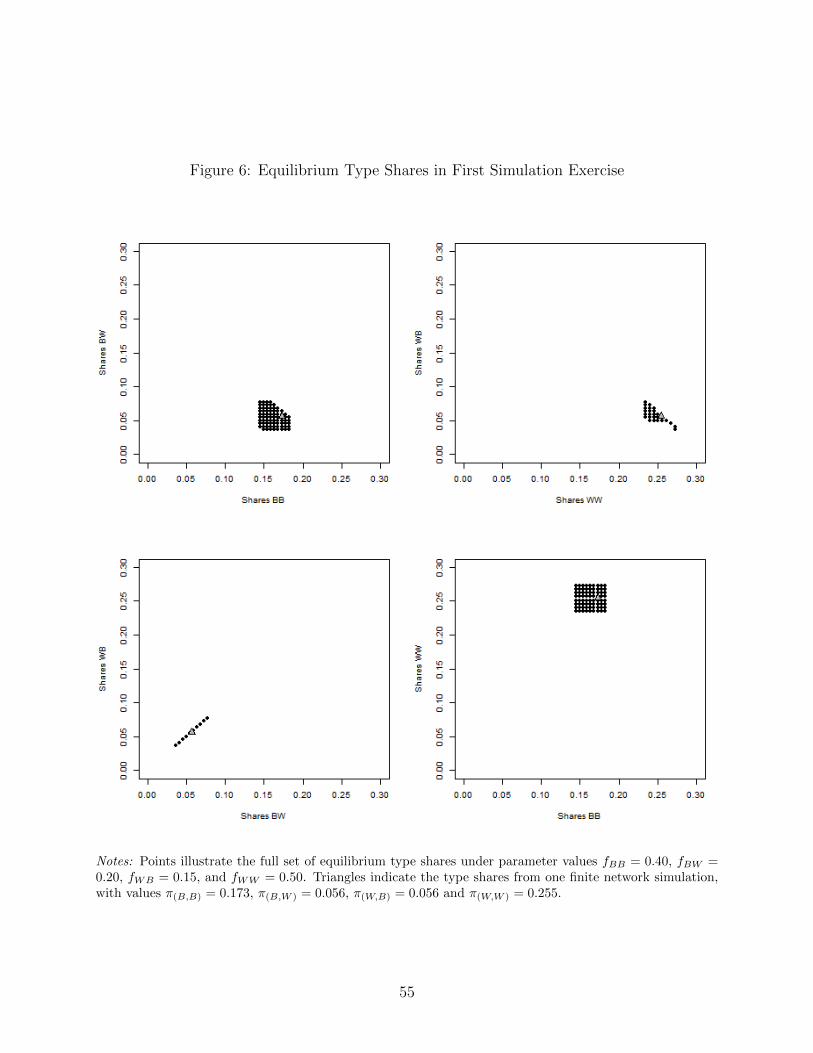
Figure 6: Equilibrium Type Shares in First Simulation Exercise

need to revise the figure, currently it shows type shares conditional on race

Notes: Points illustrate the full set of equilibrium type shares under parameter values fBB = 0.40, fBW =0.20, fWB = 0.15, and fWW = 0.50. Triangles indicate the type shares from one finite network simulation,with values π(B,B) = 0.173, π(B,W ) = 0.056, π(W,B) = 0.056 and π(W,W ) = 0.255.

55

Figure 7: Identified Set from One Finite Network in First Exercise

Notes: Points illustrate the identified set obtained using type shares from one finite network (shown withtriangles in Figure 6). Diamonds indicate true parameter values: fBB = 0.40, fBW = 0.20, fWB = 0.15,and fWW = 0.50.

56

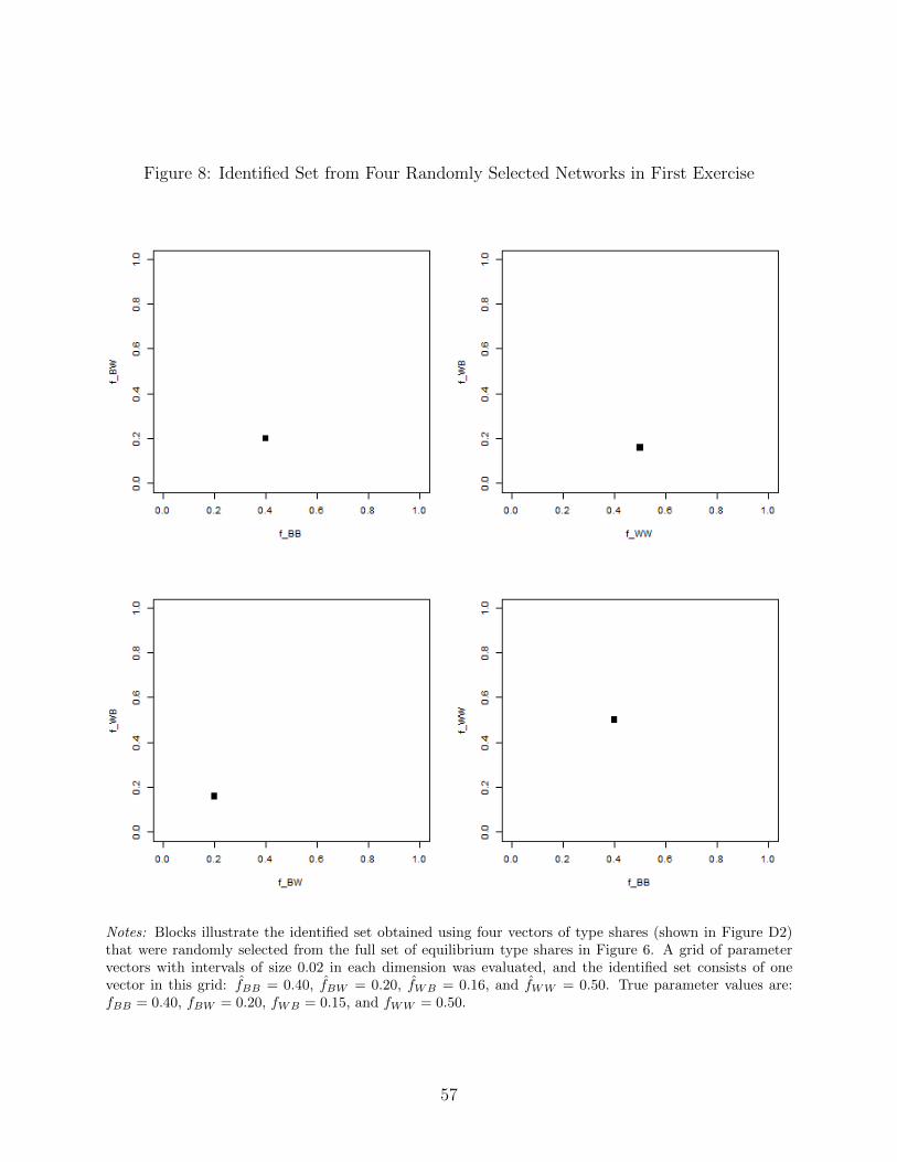
Figure 8: Identified Set from Four Randomly Selected Networks in First Exercise

Notes: Blocks illustrate the identified set obtained using four vectors of type shares (shown in Figure D2)that were randomly selected from the full set of equilibrium type shares in Figure 6. A grid of parametervectors with intervals of size 0.02 in each dimension was evaluated, and the identified set consists of onevector in this grid: fBB = 0.40, fBW = 0.20, fWB = 0.16, and fWW = 0.50. True parameter values are:fBB = 0.40, fBW = 0.20, fWB = 0.15, and fWW = 0.50.

57

Figure 9: Equilibrium Type Shares in Second Simulation Exercise

●●● ●●●

●● ●

●●●

● ●

●

●●●

●

●●

● ● ●●●●●

●

●

●●

●

●

● ●●●

●

●●

● ●●●●

●

0.00 0.05 0.10 0.15 0.20

0.0

0.2

0.4

0.6

0.8

B: isolated

W: i

sola

ted

● ●●●●●

● ●●

●

●●

●●●

●

● ●

●

●●●●●

●● ● ●

●

●

●●

●

●

●●● ●●

●●●●

●● ●●

0.00 0.05 0.10 0.15 0.20

0.0

0.2

0.4

0.6

0.8

B: B friend(s)

W: W

frie

nd(s

)

●

●

●●

●●●

●

●

●

● ●

●●

●

●

●

●

●

●●

●

●

●

●●

●

●

●●

●

●

●●

●

●

●

●

●●

●●●

●●●●

0.00 0.05 0.10 0.15 0.20

0.00

0.05

0.10

0.15

0.20

B: W friend(s)

W: B

frie

nd(s

)

● ● ●● ●●● ●●● ●●● ●● ●● ●●● ● ● ●●●●●●●● ●● ●●●● ●●● ●●● ●● ●●●

0.0 0.2 0.4 0.6 0.8 1.0

0.0

0.2

0.4

0.6

0.8

1.0

Indirect friend(s)

Mut

ual f

riend

(s)

Notes: Figure plots shares of isolated types (x: isolated) and certain combinations of other types: types withany own-race friends (x: x friend(s)), any opposite-race friends (x: y friend(s)), any indirect friends, andany mutual friends. Points represent the shares from different simulated networks, and triangles indicate theshares from the network randomly selected to use as the observation.

58

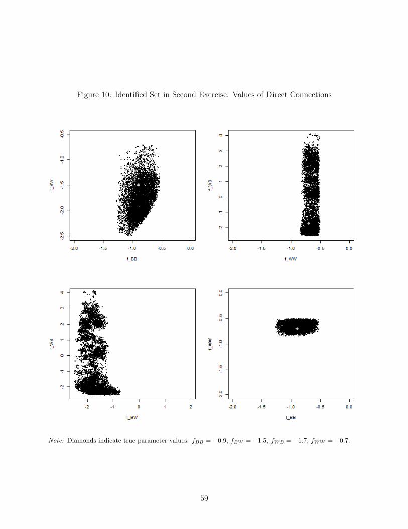
Figure 10: Identified Set in Second Exercise: Values of Direct Connections

Note: Diamonds indicate true parameter values: fBB = −0.9, fBW = −1.5, fWB = −1.7, fWW = −0.7.

59

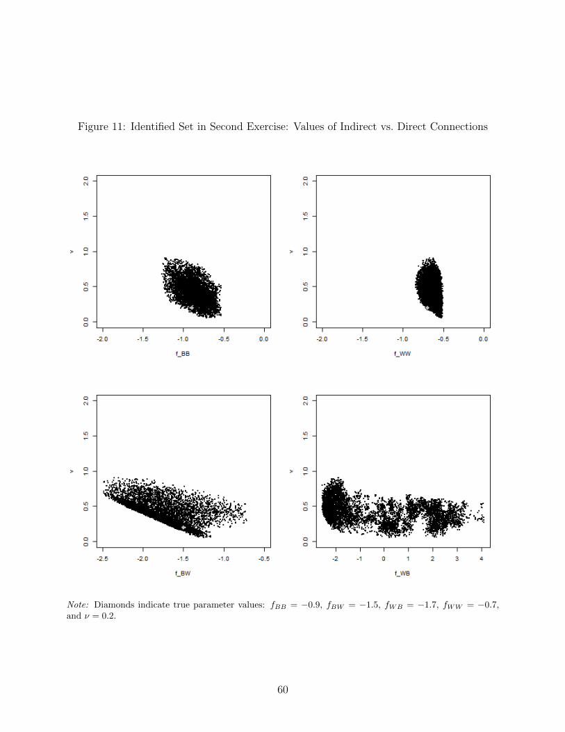
Figure 11: Identified Set in Second Exercise: Values of Indirect vs. Direct Connections

Note: Diamonds indicate true parameter values: fBB = −0.9, fBW = −1.5, fWB = −1.7, fWW = −0.7,and ν = 0.2.

60

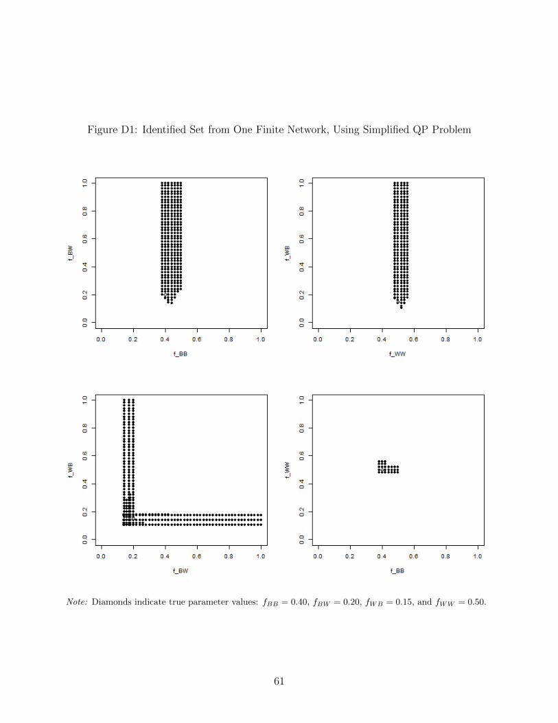
Figure D1: Identified Set from One Finite Network, Using Simplified QP Problem

Note: Diamonds indicate true parameter values: fBB = 0.40, fBW = 0.20, fWB = 0.15, and fWW = 0.50.

61

Figure D2: Type Shares in Four Randomly Selected Networks (A, B, C, D)

Notes: Letters A, B, C, D correspond to four vectors of type shares that were randomly selected from thefull set of equilibrium type shares in Figure 6. Positions of the letters indicate the values of the type shares.

62

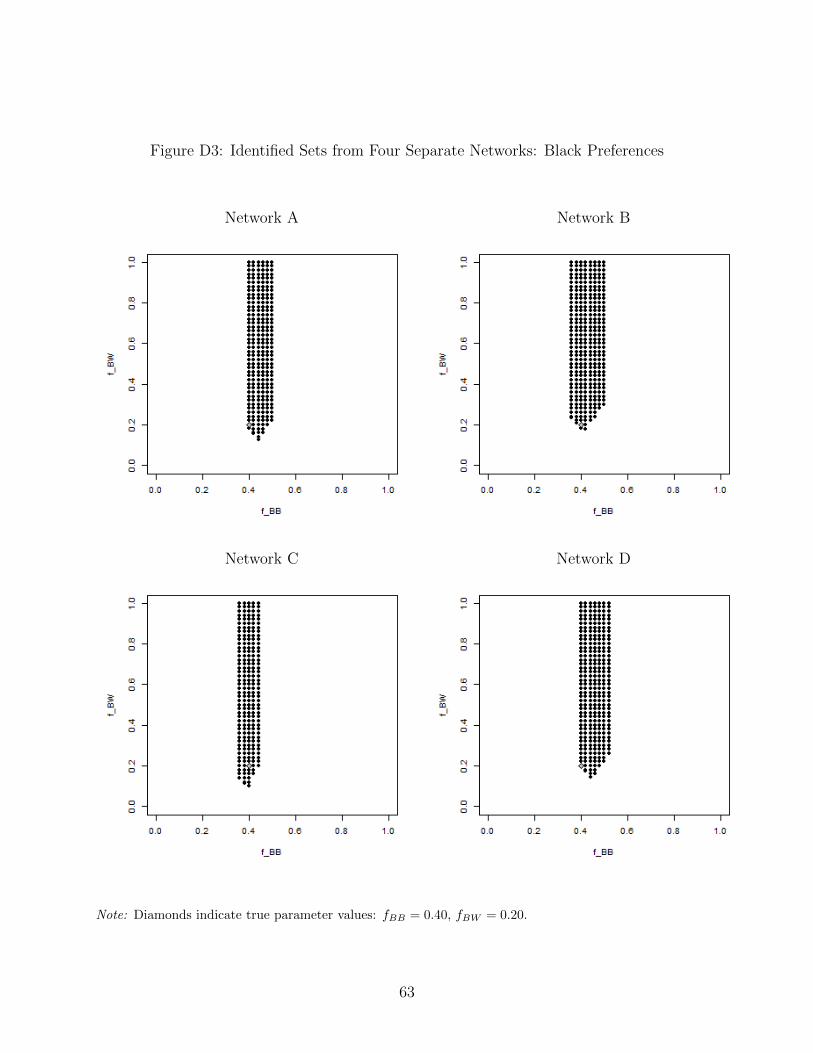
Figure D3: Identified Sets from Four Separate Networks: Black Preferences

Network A Network B

Network C Network D

Note: Diamonds indicate true parameter values: fBB = 0.40, fBW = 0.20.

63

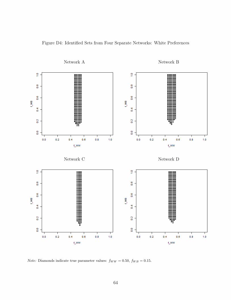
Figure D4: Identified Sets from Four Separate Networks: White Preferences

Network A Network B

Network C Network D

Note: Diamonds indicate true parameter values: fWW = 0.50, fWB = 0.15.

64

Figure D5: Degree Distribution in Second Exercise Compared with Add Health Study

0

10

20

30

40

50

0 1 2 3 4 5

Pe

rce

nta

ge o

f In

div

idu

als

Number of Links

Simulation Add Health

65