identifying multiple steady states in the design of

Scholars' Mine Scholars' Mine

Doctoral Dissertations Student Theses and Dissertations

Fall 2010

Identifying multiple steady states in the design of reactive Identifying multiple steady states in the design of reactive

distillation processes distillation processes

Thomas Karl Mills

Follow this and additional works at: https://scholarsmine.mst.edu/doctoral_dissertations

Part of the Chemical Engineering Commons

Department: Chemical and Biochemical Engineering Department: Chemical and Biochemical Engineering

Recommended Citation Recommended Citation Mills, Thomas Karl, "Identifying multiple steady states in the design of reactive distillation processes" (2010). Doctoral Dissertations. 2190. https://scholarsmine.mst.edu/doctoral_dissertations/2190

This thesis is brought to you by Scholars' Mine, a service of the Missouri S&T Library and Learning Resources. This work is protected by U. S. Copyright Law. Unauthorized use including reproduction for redistribution requires the permission of the copyright holder. For more information, please contact [email protected].

https://library.mst.edu/

https://library.mst.edu/

https://scholarsmine.mst.edu/

https://scholarsmine.mst.edu/doctoral_dissertations

https://scholarsmine.mst.edu/student-tds

https://scholarsmine.mst.edu/doctoral_dissertations?utm_source=scholarsmine.mst.edu%2Fdoctoral_dissertations%2F2190&utm_medium=PDF&utm_campaign=PDFCoverPages

http://network.bepress.com/hgg/discipline/240?utm_source=scholarsmine.mst.edu%2Fdoctoral_dissertations%2F2190&utm_medium=PDF&utm_campaign=PDFCoverPages

https://scholarsmine.mst.edu/doctoral_dissertations/2190?utm_source=scholarsmine.mst.edu%2Fdoctoral_dissertations%2F2190&utm_medium=PDF&utm_campaign=PDFCoverPages

mailto:[email protected]

IDENTIFYING MULTIPLE STEADY STATES

IN THE DESIGN OF

REACTIVE DISTILLATION PROCESSES

by

THOMAS KARL MILLS

A DISSERTATION

Presented to the Faculty of the Graduate School of the

MISSOURI UNIVERSITY OF SCIENCE AND TECHNOLOGY

In Partial Fulfillment of the Requirements for the Degree

DOCTOR OF PHILOSOPHY

in

CHEMICAL ENGINEERING

2010

Approved by

Neil L Book, Coadvisor

Oliver C Sitton, Coadvisor Douglas K Ludlow Jee-Ching Wang

Mark W Fitch

© 2010

Thomas K Mills

All Rights Reserved

iii

PUBLICATION DISSERTATION OPTION

This dissertation has been prepared in the style utilized by Computers and

Chemical Engineering. Pages 18-32 and 33-47 will be submitted for publication in that

journal. Appendices A, B, C, and D have been added for purposes normal to dissertation

writing.

iv

ABSTRACT

Global homotopy continuation is used to identify multiple steady states in ideal

reactive flash and reactive distillation systems involving a reaction of the form A+B ↔C

taking place in the liquid phase. The choice of specifications has an influence on the

existence of multiple solutions for both the flash and the column. For the flash,

specification of the heat input or withdrawal can give rise to multiplicities while

specification of the split fraction does not. Specification of one internal energy balance

variable and one external material balance variable does not produce multiplicities in the

column; however, specification of two internal energy balance variables can produce

multiplicities. This is seen to have implications for the selection of control variables for

both the flash and the column.

The effects of the relative volatility between the light and heavy components, the

forward rate constant, and the reaction equilibrium constant are studied. It is concluded

that both the relative volatility spread and the equilibrium constant exhibit threshold

values, below which only singular solutions are obtained. Above this threshold,

multiplicities are to be found. The rate constant also affects the appearance of multiple

solutions, but the multiplicities are found in regions bounded above and below by regions

producing only singular solutions.

The cause of multiplicities in the idealized system studied is seen to be the

interaction between consumption and creation of species by reaction and transfer of

material between phases. The reaction rate appears to be the major contributor to this

effect because it is able to reverse direction, assuming either positive or negative values.

v

ACKNOWLEDGMENTS

The author is indebted to advisors Dr Neil Book and Dr Oliver Sitton for their

advice and guidance during this project, and to committee members Dr Douglas Ludlow,

Dr Jee-Ching Wang, and Dr Mark Fitch for their support and encouragement. A debt of

thanks is also owed to other members of the Chemical Engineering department, past and

present, for their encouragement along the way.

Additionally, sincere thanks are due to the author’s wife Janice, son Thomas Jr,

and father Horace Mills, whose encouragement and patience have made this project

possible.

vi

TABLE OF CONTENTS

Page

PUBLICATION DISSERTATION OPTION.................................................................... iii

ABSTRACT....................................................................................................................... iv

ACKNOWLEDGMENTS .................................................................................................. v

LIST OF ILLUSTRATIONS........................................................................................... viii

LIST OF TABLES............................................................................................................. ix

NOMENCLATURE ........................................................................................................... x

SECTION

1. INTRODUCTION...................................................................................................... 1

1.1. CHEMICAL / THERMODYNAMIC MODEL ................................................. 1

1.2. COLUMN MODEL AND SOLUTION ALGORITHM .................................... 3

2. LITERATURE REVIEW........................................................................................... 5

2.1. REACTIVE DISTILLATION APPLICATION................................................. 5

2.2. GRAPHICAL AND ALGEBRAIC MODELS................................................... 5

2.3. SIMULATIONS OTHER THAN WITH HOMOTOPY CONTINUATION .. 11

2.4. HOMOTOPY METHOD DEVELOPMENT ................................................... 15

2.5. HOMOTOPY METHOD APPLICATION ...................................................... 17

PAPERS

I. MULTIPLE STEADY STATES IN THREE-COMPONENT REACTIVE DISTILLATION: EFFECT OF OPERATING PARAMETERS............................ 18

ABSTRACT............................................................................................................. 18

1. INTRODUCTION............................................................................................ 18

2. THE REACTIVE FLASH................................................................................ 20

3. THE REACTIVE COLUMN ........................................................................... 23

4. CONCLUSIONS.............................................................................................. 29

NOMENCLATURE ................................................................................................ 30

vii

REFERENCES ........................................................................................................ 31

II. MULTIPLE STEADY STATES IN THREE-COMPONENT REACTION SYSTEMS: EFFECT OF COMPONENT PHYSICAL PROPERTIES ................ 33

ABSTRACT............................................................................................................. 33

1. INTRODUCTION............................................................................................ 33

2. THE REACTIVE FLASH................................................................................ 35

3. THE REACTIVE COLUMN ........................................................................... 39

4. CONCLUSIONS.............................................................................................. 42

NOMENCLATURE ................................................................................................ 45

REFERENCES ........................................................................................................ 46

SECTION

3. CONCLUSIONS...................................................................................................... 48

APPENDICES

A. COMPUTER PROGRAMS USED FOR THIS STUDY....................................... 50

B. REACTIVE DISTILLATION PROGRAM SOURCE CODE............................... 79

C. REACTIVE FLASH PROGRAM SOURCE CODE ........................................... 130

D. HOMOTOPY CONTINUATION SOLVER SOURCE CODE........................... 159

BIBLIOGRAPHY........................................................................................................... 186

VITA .............................................................................................................................. 192

viii

LIST OF ILLUSTRATIONS

Page

PAPER I

Figure 1 - Reactive flash ............................................................................................ 20

Figure 2 – Reactive flash with vapor-to-feed ratio specified..................................... 23

Figure 3 – Reactive flash with heat duty specified .................................................... 24

Figure 4 - Reactive column ........................................................................................ 24

Figure 5 – Reactive distillation with specified boilup and bottoms rates .................. 26

Figure 6 – Reactive distillation with boilup and reflux rate specified ....................... 27

Figure 7 – Component A liquid compositions with boilup and reflux rate specified 28

Figure 8 – Component B liquid compositions with boilup and reflux rate specified 28

Figure 9 – Component C liquid compositions with boilup and reflux rate specified 29

PAPER II

Figure 1 – Reactive flash............................................................................................ 35

Figure 2 - Conversion versus Damkohler number for a range of species A relative volatilities .................................................................................................. 38

Figure 3 - Conversion versus Damkohler number for a range of rate constant values......................................................................................................... 38

Figure 4 - Conversion versus Damkohler number for a range of equilibrium constant values .......................................................................................... 39

Figure 5 - Reactive column ........................................................................................ 41

Figure 6 - Conversion versus distillate to feed ratio for a range of relative volatilities .................................................................................................. 43

Figure 7 - Conversion versus distillate to feed ratio for a range of values of the forward rate constant................................................................................. 43

Figure 8 - Conversion versus distillate to feed ratio for a range of values of the reaction equilibrium constant ................................................................... 44

ix

LIST OF TABLES

Page

SECTION 1

Table 1.1 - Some three-component reactive distillation systems................................. 2

PAPER I

Table 1 – Commercial reactive distillation systems for A+B ↔ C ........................... 19

Table 2 - Operating parameters for base case flash ................................................... 22

Table 3 - Material parameters for base flash case...................................................... 22

Table 4 - Operating parameters for base distillation case .......................................... 26

Table 5 - Component parameters for base distillation case ....................................... 26

PAPER II

Table 1 - Some three-component reactive distillation systems.................................. 35

Table 2 - Operating parameters for base case flash ................................................... 37

Table 3 - Material parameters for base flash case...................................................... 37

Table 4 - Operating parameters for base distillation case .......................................... 41

Table 5 - Component parameters for base distillation case ....................................... 41

x

NOMENCLATURE

Symbol Description

Ai, Bi constants for component vapor pressure expression

D/F vapor overhead to feed ratio

EA reaction activation energy, J/mol

Fj molar bulk feed rate to stage j, mol/time

fij component i feed rate to stage j, mol/time

hj liquid holdup on stage j, mol

H stream enthalpy, J/mol

∆Hr heat of reaction, J/mol

∆Hv heat of vaporization, J/mol

Kij component i vapor-liquid distribution coefficient

kf,0 reaction forward rate constant pre-exponential

kf reaction forward rate constant at temperature T

Ke,0 reaction equilibrium constant pre-exponential

Ke reaction equilibrium constant at temperature T

Lj molar liquid rate, mol/time

lij component i liquid rate

p*i component i vapor pressure, bar

P pressure, bar

Q heat added to the flash, J/time

R gas constant

rij component i production, moles per unit time

Slj liquid side-draw from stage j

Svj vapor side-draw from stage j

Tj temperature, K

Vj molar vapor rate, mol/time

vij component i vapor rate, mol/time

xij liquid mole fraction i

yij component i vapor mole fraction

xi

Greek letters

αi component i volatility relative to the heavy component

Φ vapor-to-feed ratio

ηj Murphree efficiency

λj reaction extent, mol/time

υi component i stoichiometric coefficient

Θ unit of time

Subscripts

i component index

j stage index

l liquid phase

v vapor phase

1. INTRODUCTION

Most commercial chemical processes feature at least one chemical reaction, along

with one or more separations, commonly distillation. Distillation has been an important

part of chemical processing for a very long time; however, the rapid growth in computing

capabilities in the last few decades has enabled a corresponding increase in the

sophistication of design calculations. This in turn has allowed the use of more complex

configurations to satisfy demands for increased performance and economy. In particular,

reactive distillation, in which both chemical reaction and the separation of products from

byproducts and residual reactants take place in the same equipment, has received

increasing attention in recent years (Malone and Doherty 2000).

One of the issues needing to be addressed in reactive distillation is the potential

existence of multiple steady states, which has been observed both in laboratory and plant

practice as well as in design calculations (Mohl, Kienle, Gilles et al. 1999). Output

multiplicities, in which a process may exhibit differing performance profiles for

apparently identical operating parameters, are particularly troublesome from the

standpoint of design and control. Standard design calculation techniques for such

processes may converge to different solutions, depending on the starting estimates used

for process variables, but are typically able to find only a single profile for any given set

of inputs (Taylor and Krishna 2000). When constructed on the basis of these design

methods, the reactive distillation unit may not exhibit the expected profile, depending on

the initial conditions at startup or the states imposed by transients during the operation of

the unit. Performance and/or safety issues can be the result.

1.1. CHEMICAL / THERMODYNAMIC MODEL

Of the many systems for which reactive distillation has been studied or

commercialized, several involve reactions of the form A+B↔C (Luyben and Yu 2008).

A small sampling of these systems is presented in Table 1.1.

2

Table 1.1 - Some three-component reactive distillation systems

For these systems, the mass-action rate law may be expressed as

( )( )/( / ),0 ,0/ rA H RTE RT

f A B C er k e x x x K e −∆−= −

Systems with reactions of the form 2A ↔ C or A ↔ B + C and with similarly

structured rate laws have also been studied or commercialized.

For modeling the vapor-liquid equilibrium behavior of the system, it is desirable

to represent the system with a minimal number of specified parameters. For this reason, it

is convenient to assume that Raoult’s law and the Clausius-Clapeyron equation are

descriptive. From Raoult’s law

yi = xi(pi*/P)

where yi and xi are the vapor and liquid mole fractions of component i, respectively, P is

the total pressure, and pi*is the vapor pressure of component i. The Clausius-Clapeyron

equation gives

ln(pi*/pi

*0) = (∆HVi/R)(1/T0 – 1/T)

where ∆HVi is the component i heat of vaporization, R is the gas constant, pi*0 is the

component i vapor pressure at reference temperature T0, and T is the system temperature.

This reduces to the more useful form

A B C

acetaldehyde acetic anhydride vinyl acetate

acetone hydrogen isopropanol

benzene ethylene ethylbenzene

isoamylene water tert-amyl alcohol

methanol isobutene methyl tert-butyl ether

methanol isoamylene tert-amyl methyl ether

3

ln pi* = [lnpi

*0+∆HVi/RT0]-∆HVi/RT = Ai-Bi/T

where Ai = lnpi*0+∆HVi/RT0 and Bi = ∆HVi/R. These values are easily determined by

setting the reference temperature T0 to the normal boiling point of the component.

Making the assumption that ∆HV1 = ∆HV2 = ∆HV3 = …= ∆HVn gives

lnαij = ln(pi*/pj

*)=(∆HV/R)(1/Tbi – 1/Tbj)

which yields

Tbj = 1/[1/Tbi –Rlnαij/∆HV]

Assuming that both vapor and liquid heat capacities are negligible and that enthalpies are

zero at the saturated liquid reference state further simplifies the computations.

1.2. COLUMN MODEL AND SOLUTION ALGORITHM

Perhaps the most straightforward approach to modeling distillation columns is the

simultaneous correction scheme documented by Naphtali and Sandholm (1971), in which

each stage is represented by a set of equations consisting of component material balances,

stage energy balance, stream component summations, and component vapor-liquid

distributions. For distillation with reactions occurring on the stages, Taylor and Krishna

(2000) revised the equation set to incorporate the production or consumption of each

component into the material balance functions:

Material Balance: (1+Sl,j)/li,j + (1+Sv,j)vi,j –li,j-1 –vi,j+1 –fi,j –ri,j = 0

Equilibrium Functions: (ηi,jKi,j)li,j/Lj – vi,j/Vj + ((1-ηi,j)vi,j+1)/Vj+1 = 0

Energy Balance: (1+Sl,j)Hl,j + (1+Sv,j)Hv,j –Hl,j-1 –Hv,j+1 –Hf,j –Q,j = 0

Traditionally, the set of equations describing a column has been solved by a

locally convergent approach such as Newton’s method. One characteristic of these

methods is that they are able to find only a single solution. Where the possibility of

multiple solutions is an issue, a global solving algorithm is needed. Methods have been

developed for finding multiple solutions to reactive distillation problems; however, these

4

methods have been predominantly graphical or algebraic (Bekiaris and Morari 1996;

Bessling, Schembecker, and Simmrock 1997; Dalal and Malik 2003), and are thus limited

in the precision they can offer and the number of species involved in the problems they

can address. Homotopy continuation has been found useful because of its robustness and

its ability to locate multiple solutions (Wayburn and Seader 1987; Kuno and Seader

1988; Lee and Dudukovic 1998; Sun and Seider 1995; Choi, Harney, and Book 1996). In

the most common application of this approach, a vector of initial guesses x0 is mapped to

solution vectors x* by a homotopy function h(x,t) = tf(x) + (1-t)g(x0) where g(x0) is a

vector of “simple” functions, f(x) is a vector of the functions to be solved, and t is the

homotopy parameter. The solutions of h(x,t) = 0 form a homotopy path, which maps the

solution of g(x0)= 0 to a solution of f(x*)= 0 as the value of t is varied from 0 to 1.

Multiple solutions of f(x) are found by global homotopy continuation, in which the

homotopy path is exhaustively traced to locate solutions of f(x)= 0. Algorithms have been

developed (Choi 1990; Choi, Harney, and Book 1996) to overcome the possibility of

missing solutions by skipping from one segment of the homotopy path to another.

However, Choi and Book (1991) demonstrated that all solutions may not be located on

the single homotopy path emanating from the starting point. Therefore, these methods do

not absolutely guarantee determination of all solutions.

Nonetheless, much of the published work in this area has dealt with specific

systems of more-or-less nonideal components (Kovach III and Seider 1987; Singh et al.

2005). The problem of identifying parametric combinations or ranges of values for which

multiplicities do or do not appear in generalized ideal systems has yet to receive adequate

attention.

5

2. LITERATURE REVIEW

2.1. REACTIVE DISTILLATION APPLICATION

Harmsen (2007) discussed the increased application of reactive distillation,

primarily in the last two decades. He cited more than 150 processes, in the range of 100-

3000 ktonne/yr operating worldwide. He concluded that reactive distillation has become

an established unit operation, and should be considered a front-runner in the field of

process intensification.

Hoyme (2004) conducted parametric studies of several ideal reactive distillation

systems. On the basis of these studies, he developed a set of heuristics for predicting the

economic feasibility of a given reactive distillation process. He identified reaction

equilibrium constant, volatility order, relative volatility, and reflux ratio as key

parameters in economic feasibility estimation.

2.2. GRAPHICAL AND ALGEBRAIC MODELS

Barbosa and Doherty (1988a) presented a set of transformed composition

variables to simplify design equations for single-feed reactive distillation columns. A

method of calculating minimum reflux ratios for reactive columns was developed, based

on these simplified equations.

Equations describing the distillation of homogeneous reactive mixtures were

derived by Barbosa and Doherty (1988b), and were used to compute residue curve maps

for ideal and non-ideal systems. It was shown that distillation boundaries could be either

created or eliminated by allowing the mixture components to react.

Karimi and Inamdar (2002) noted that, although many systems are described by

equations that cannot be reduced to a single equation, much of the work on bifurcation

diagrams and identification of steady state multiplicities relies on either the assumption

that such systems are reducible or some mathematical technique exists to reduce them.

They presented a perturbation method for dealing with multiple equations without

reduction, and used their method to study branching and stability of steady states near a

singularity.

6

Monnigmann and Marquardt (2003) presented an approach to the optimization

based design of processes in which uncertainty in some process parameters exists. Their

approach operates by placing a lower bound on the distance of the nominal operating

point from stability and feasibility boundaries in the space defined by the uncertain

parameters. They discuss their method in the context of optimizing a process known to

have a nontrivial stability boundary caused by steady state multiplicity and sustained

oscillation.

Baur, Taylor, and Krishna (2003) compared the use of heterogeneous and pseudo-

homogeneous reaction kinetic models in preparing a bifurcation analysis of a reactive

distillation for the synthesis of t-amyl methyl ether. They concluded that the two models

show similar performance, both indicating the possibility of multiple steady states. They

attributed difference in performance to imprecision in the knowledge of liquid holdup and

other hydrodynamic factors.

Barbosa and Doherty (1987a) derived expressions for the partial derivatives of

intensive properties that characterize equilibrium states in two-phase systems with one

chemical reaction. They found necessary and sufficient conditions for the occurrence of

azeotropic transformation, and presented conditions under which reactive azeotropes are

not equivalent to stationary points in the equilibrium surfaces.

Barbosa and Doherty (1987b) presented a transformed set of composition

variables for representing phase diagrams where chemical reaction is present. They make

the claim that this set of variables is superior to mole fractions in several respects, and

give examples of phase diagrams to illustrate the claimed advantages.

Barbosa and Doherty (1988c) presented phase diagrams for simultaneous

chemical reaction and phase equilibrium for both ideal and non-ideal systems. They

showed that even for ideal mixtures, reactive azeotropes can occur. In addition, they

concluded that for such reactive azeotropes to exist, volatilities of the reactants must be

either all higher or all lower than the volatilities of the products.

Bekiaris et al. (1993) studied multiple steady states in homogeneous azeotropic

distillation. Under the conditions of infinite reflux and an infinite number of trays

(∞/∞ analysis), they constructed bifurcation diagrams with distillate flow as the

7

bifurcation parameter, and derived necessary conditions for the existence of multiple

steady states.

Fien and Liu (1994) presented a review of published work on the use of ternary

composition diagrams and residue curve maps for the analysis and design of azeotropic

separation processes. Their analysis sought to clarify some contradictions in prior work,

and highlighted the usefulness of this approach for preliminary system design.

Ung and Doherty (1995a) showed that the Gibbs free energy for reacting mixtures

can be expressed as an unconstrained function of a set of transformed composition

variables. From this, they developed a simplified representation of equilibrium and

stability conditions in reactive systems that is similar to the non-reacting case.

Ung and Doherty (1995b) showed that in a transformed composition space,

conditions for azeotropy in reactive mixtures take the same functional form as in non-

reactive mixtures. However, reactive azeotropes generally do not correspond to points of

equal mole (or mass) fraction in the coexisting phases.

Ung and Doherty (1995c) introduced a set of composition variables for evaluating

phase equilibria in multicomponent, multireaction systems. They showed that their

transformed variables simplified analysis by reducing the dimensionality of the problem.

They found that reactive azeotropes occur at points of equal transformed composition in

coexisting phases, but not at points of equal mole fraction.

Ung and Doherty (1995d) derived the differential equations describing simple

distillation of mixtures with multiple chemical reactions. They found that the results are

conveniently expressed in terms of composition coordinates transformed to reduce the

dimensionality of the problem. From this, they prepared residue curve maps which

provide visualization of the combined equilibria, and show the presence of reactive

azeotropes as well as non-reactive azeotropes which survive the reactions.

Bekiaris, Meski, and Morari (1996) used the assumptions of infinite reflux ratio

and infinite number of trays to construct bifurcation diagrams for ternary azeotropic

systems. With distillate flow rate as the bifurcation parameter, they demonstrated that

these diagrams could be used to predict the occurrence of multiple steady states. They

also showed relevant implications for cases with finite reflux and a finite number of trays.

8

Bekiaris and Morari (1996) extended a previously presented method of analysis to

quaternary mixtures, and elaborated on the implications for column design and

simulation. They discussed the effect of thermodynamic phase equilibrium on the

existence of multiplicities, and identified classes of mixtures for which multiplicities are

inherent and robust. Finally, they discussed issues arising from their analysis that are

relevant to the use of commercial simulators for computing the composition profiles of

azeotropic distillation columns.

Bessling et al. (1997) studied the concept of residue curve maps based on

transformed composition variables. From this study, they developed conditions under

which a combination of reactive and non-reactive sections is needed within a given

column.

Gehrke and Marquardt (1997) demonstrated the application of singularity theory

to the analysis of a one-stage reactive distillation, in order to study the causes of multiple

steady states. They identified causes which are common to non-reactive processes, as

well as those that are connected to the interaction between chemical reaction and phase

equilibrium.

Guttinger and Morari (1997) reviewed and demonstrated the ∞/∞ analysis of

Bekiaris et al. (1993) for multicomponent azeotropic mixtures. They then extended the

analysis by combining it with a singularity analysis to treat additional azeotropic systems,

and by combining it with reactive residue curves to treat problems involving reaction. In

addition, they related known multiplicities for the MTBE process to causative physical

phenomena.

Karpilovskiy, Pisarenko, and Serafimov (1997) used distillation line diagrams and

reaction stoichiometry to derive a criterion for predicting multiple steady states in a

single-product reactive distillation. Their criterion successfully predicted multiplicity for

butyl acetate synthesis, which prediction was confirmed by further analysis.

Song et al. (1998) studied the influence of heterogeneous catalysis on the

kinetically controlled esterification of acetic acid with methanol in a reactive distillation

system. They noted the role of pressure in regulating liquid boiling point and thus

reaction temperature. They experimentally measured residue curves, and compared the

results with predictions from a kinetic model.

9

Guttinger and Morari (1999a) present a method for predicting the existence of

multiple steady states in columns consisting solely of reactive stages, for the limiting case

of infinite column length and infinite internal flows. They applied geometric conditions

to identify the region of feed compositions leading to multiplicities.

Guttinger and Morari (1999b) developed a graphical method for predicting

multiple steady states in columns containing both reactive and nonreactive sections

(“hybrid columns”). This extended their development of a method for analyzing columns

having only reactive stages (“nonhybrid columns”). They showed their method to be

capable of predicting the existence of, and feed regions giving rise to, multiple steady

states.

Reder, Gehrke, and Marquardt (1999) applied the geometric ∞/∞ analysis to

esterification reactions occurring in distillation columns, and transferred their findings to

rigorous reactive column models, weakening the assumptions of infinite reflux and

column length. They showed that where the ∞/∞ analysis can predict an infinite number

of steady states, relaxation of the assumptions reduces the prediction to a finite number,

and that at relatively small values of reaction rate, column length, or reflux rate, the

multiplicities reduce to unique solutions.

Bekiaris et al. (2000) studied the observation of output multiplicities in numerical

simulation of heterogeneous azeotropic distillation columns. They concluded that the

accuracy of the thermodynamic description is a key factor in determining whether

multiplicities can be observed. In addition, they studied reported multiplicities, and

derived relationships to identify causative physical phenomena.

Jalali-Farahani and Seader (2000) investigated stability in nonideal chemical

systems where reactions occur in more than one phase. They used a homotopy

continuation method to identify solutions, and stability criteria were applied to determine

the number of stable phases at equilibrium.

Melles et al. (2000) studied the effect of tray holdup in continuous kinetically

controlled reactive distillation columns. They concluded that using tray holdup as a

parameter aided the design and optimization of such columns.

Kenig et al. (2001) studied the synthesis of ethyl acetate by homogeneously

catalyzed reactive distillation. They identified feasible configurations through the use of

10

residue curve map techniques, then used a rate-based simulator to predict concentrations

and other relevant process variables. They found substantial agreement between

experimental data and their predicted temperature and composition profiles.

Rodriguez, Zheng, and Malone (2001) studied the steady state behavior of an

isobaric, adiabatic reactive flash for a two component system. They noted that vapor-

liquid equilibrium can create or remove steady state multiplicities, relative to a single

phase reactor. They related the presence of multiple steady states to a dimensionless

parameter formed from the heats of reaction and vaporization along with the

compositions in the system.

Rodriguez (2002) noted that, while combining a reaction step with a separation

step can be economically efficient, it also reduces the degrees of freedom available for

controlling the system. He applied bifurcation and singularity theory to derive algebraic

expressions that describe the possibility of steady state multiplicities. His work

considered both the reactive (multistage) column and the two-phase reactor (reactive

flash).

Rodriguez, Zheng, and Malone (2002) studied steady state solutions for an

isobaric, adiabatic, reactive flash, and showed that the existence of the second phase

affects the presence or absence of steady state multiplicities. They related the existence of

multiple steady states to a dimensionless quantity derived from the heats of reaction and

vaporization along with the vapor-liquid equilibrium behavior.

Huss et al. (2003) illustrated an approach to the design of reactive distillation

columns, using methyl acetate production as an example. They demonstrated that in the

limit of both phase and reaction equilibrium, there are both minimum and maximum

reflux limits, and that multiple steady states persist throughout the range of feasible reflux

ratios. For finite reaction rates, they showed that desired compositions are achievable

over a wide range of reaction rates, and that multiplicities occur at high reflux ratios

beyond the range of normal operation.

Rodriguez, Zheng, and Malone (2004) noted that steady state multiplicity is

caused by interaction between reaction and separation in systems with sufficiently large

activation energy and boiling temperature versus composition gradient. They established

necessary conditions for multiplicity in an isobaric flash with constant split fraction, and

11

determined that multiplicity is possible in endothermic systems as well as those with a

small heat of reaction.

2.3. SIMULATIONS OTHER THAN WITH HOMOTOPY CONTINUATION

Naphtali and Sandholm (1971) presented an approach to separation calculations in

which component material balances, enthalpy balances, and equilibrium relationships

were arranged to be solved simultaneously. Their construct formed the basis which others

subsequently extended to include the effect of chemical reaction.

Taylor and Krishna (2000) presented a comprehensive review of models for

reactive distillation, noting that multiple steady states had been predicted by theoretical

studies as early as the 1970’s. They cited several models which had been used to make

these predictions, primarily through altering the parameters of standard simulation

models or use of singularity theory or bifurcation analysis. Their review covered only

real-component systems, and noted several experimental studies verifying these

predictions.

Seferlis and Grievink (2001) presented a method for screening control

configurations to identify manipulated variables that perform poorly in the presence of

multiple disturbances and parameter variations. In particular, they developed a

comparison between reactive distillation configurations and conventional reactor-

separator schemes.

Tang et al. (2005) studied the esterification of acetic acid using five different low

molecular weight alcohols, and identified three different types of flowsheets. For each

flowsheet type, they presented a design procedure and explored economic potential.

Grosser, Doherty, and Malone (1987) proposed a model for reactive distillation in

a system where extreme purity is required in the overhead vapor. They concluded that

economical operation of such systems is enhanced by the use of a reactive entrainer.

They also presented guidelines for the use of reactive entrainers in the separation of

closely boiling mixtures.

Hua, Brennecke, and Stadtherr (1996) demonstrated an initialization independent

interval analysis technique for reliably solving phase stability problems. They concluded

12

that their technique, properly implemented, guarantees that all correct solutions have

been found.

Reneaume, Meyer, Letourneau, and Joulia (1996) described an approach to phase

equilibrium problems in which they found Gibbs energy minima by resolving a mixed

integer nonlinear programming problem into nonlinear programming subproblems.

Global optima for each subproblem were then found by homotopy continuation.

Sneesby, Tade, and Smith (1997, 1998) discussed three types of steady state

multiplicity, and the implications of each for column control. They concluded that input

multiplicity, or the existence of the same output for several different sets of inputs, placed

restrictions on the selection of controlled variables. Output and pseudo-multiplicities

were thought to have less significant impacts, but were seen to influence the choice of

control structure and operating region.

Okasinski and Doherty (1998) presented a design methodology for kinetically

controlled reactive distillation columns featuring a single liquid phase reaction and

nonideal vapor-liquid equilibrium. They considered their method to be useful for

developing a set of feasible designs over a range of design specifications, and provided

several examples of its application, including one in which the use of reactive distillation

removed a distillation boundary normally existing in the system being separated.

Mohl et al. (1999) studied the dynamic behavior of reactive distillation columns

for the production of methyl t-butyl ether and t-amyl methyl ether, with an emphasis on

steady state multiplicity as identified by bifurcation analysis of pilot plant columns.

Sources and physical causes of multiple steady states were discussed, as were some of

their implications.

Peng et al. (2002) compared equilibrium and rate-based models for packed

reactive distillation columns to produce tert-amyl methyl ether and methyl acetate. Both

models gave good agreement with experimental data, and predicted the existence of an

optimum pressure and reflux ratio. The rate-based model was found to be much more

complicated, and more difficult to converge, than the equilibrium model.

Dalal and Malik (2003) applied an optimization algorithm for systems of

nonlinear equations to study methanol-propanol and ethanol-water-benzene columns.

13

They were able to find multiple solutions in both cases, but concluded that a more robust

solver would represent an improvement.

Waschler, Pushpavanam, and Kienle (2003) analyzed the behavior of two-phase

reactors under boiling conditions. Focusing on a simple reaction of the form A →B, they

identified three necessary conditions for the existence of steady state multiplicities: the

reactant A must be the light component, the boiling point difference between A and B has

to be sufficiently large, and the order of the reaction must be less than a measure of the

self-inhibition of the reaction driven by phase equilibrium.

Yermakova and Anikeev (2005) constructed a model of a two-phase CSTR, or

reactive flash, for the liquid phase hydrogenation of benzene, under the assumption of

phase equilibrium. They demonstrated that under certain conditions, there exists the

possibility of a multiplicity of solutions, which were attributed to nonlinearity of the

kinetic reaction expressions and nonideality of the reacting mixture.

Yang et al. (2006) used the ASPEN PLUS simulation package to study reactive

distillation processes for ethylene glycol and ethyl t-butyl ether, with liquid holdup

volume and boilup ratio as parameters. Through the use of different initial guesses, they

were able to demonstrate steady state multiplicities for both processes.

Qi and Sundmacher (2006) investigated reactive distillation for the production of

high purity isobutene and diisobutene by dehydration of t-butyl alcohol. They noted that

mild processing conditions, high per-pass conversion, and high selectivity were

advantages offered by reactive distillation. Their analysis included examination of the

influence of important process parameters.

Calvar, Gonzalez, and Dominguez (2007) studied the kinetics of the esterification

of acetic acid with ethanol, using both heterogeneous and homogeneous catalyst systems.

Their study was carried out using a packed bed reactive distillation column, and included

an analysis of the effects of feed composition and reflux ratio.

Rovaglio and Doherty (1990) developed a dynamic model for heterogeneous

azeotropic columns which was able to detect and account for multiple liquid phases on

trays at each instant of time. They demonstrated the model by simulating the distillation

of mixtures of ethanol, water, and benzene. They showed their results to be in substantial

14

agreement with prior work, and that the system under study can be expected to exhibit

multiple steady states, complex dynamic behavior, and parametric sensitivity.

Jacobsen and Skogestad (1991) discussed two causes of multiple steady states in

ideal two-product distillation. For systems specified in mass or volume units, they

concluded that the transformation to molar units can become singular, resulting in

multiple solutions. For units specified in molar units with an energy balance included in

the model, their conclusion was that multiple solutions were caused by interaction

between flows and compositions.

Jacobs and Krishna (1993) used a steady state equilibrium stage model to simulate

a reactive distillation column for the production of methyl t-butyl ether. For identical

configuration and feed specifications, they obtained two distinct results, corresponding to

high and low conversion of isobutene. They showed that these two results were

associated with residue curves having their starting points in distinctly different

composition regions.

Baur et al. (2000) used two case studies to compare the equilibrium stage model

with a nonequilibrium model which uses mass transfer rates across the vapor-liquid

interface for modeling reactive distillation columns. It was shown that, while multiple

steady states are exhibited in both approaches, the “window” for their occurrence is

significantly smaller in the nonequilibrium case. It was also observed that some of the

multiplicities found by the equilibrium approach could not be achieved in practice due to

physical constraints.

Kumar et al. (2001) simulated a reactive distillation column for producing MTBE.

They observed two steady states, one having high conversion at relatively low

temperature and the other having lower conversion at relatively high temperature. They

also studied the effects of methanol feed tray location, reflux ratio, catalyst loading, and

other parameters on overall conversion and product purity.

Chen et al. (2002) developed a model for kinetic effects in reactive distillation,

using a Damkohler number as the key parameter. For methyl t-butyl ether synthesis and t-

amyl methyl ether synthesis, they traced solution branches as functions of the Damkohler

number, reboil ratio, or reflux ratio, and found agreement with prior work at the reaction

equilibrium limit. For the t-amyl methyl ether system, they found that multiplicities were

15

present in the kinetic regime, but disappeared above a critical value of the Damkohler

number.

Lucia and Feng (2003) investigated a geometric terrain method for finding all

solutions and singular points for chemical process simulation problems. They concluded

that their method provided reliable and efficient performance, which was seen to be

superior to differential arc homotopy continuation for some problems which exhibited

parametric disconnectedness.

Svandova et al. (2009) compared the performance of equilibrium and non-

equilibrium models for identifying hazardous situations or operability problems in

reactive distillation columns. In particular, they studied the ability of the two models for

predicting multiple steady states that can be the cause of operability issues. They

observed that, while both models predict multiplicities, the non-equilibrium model is

more realistic but requires more parameters as input and is thus more susceptible to errors

in the input information.

2.4. HOMOTOPY METHOD DEVELOPMENT

Taylor et al. (2003) presented a comparison of rate-based and equilibrium models

for nonreactive distillation. They concluded that, while much more complex than the

equilibrium models, rate-based models become more feasible as available computing

power increases, and that for definitive computations on existing columns, they should be

used in preference to equilibrium models.

Kovach and Seider (1987) presented an algorithm for simulating three-phase

azetropic distillation towers and their associated phase separators. Their algorithm

utilized a homotopy continuation method, with extensions to avoid limit points when

multiple solutions were encountered or when two liquid phases exist on the trays.

Extensions were also added to perform parametric studies by tracking solution paths.

They demonstrated the ability of the algorithm to detect regions where multiple solutions

exist, some of which had not been previously identified.

Vadapalli and Seader (2001) composed a method for incorporating an addition to

standard process simulators which are normally only able to find single solutions, so that

16

these simulators are able to trace a solution path with respect to some input parameter,

thus finding multiple solutions.

Wayburn and Seader (1987) applied homotopy continuation methods to the

solution of difficult flowsheeting and design problems involving sets of simultaneous

nonlinear equations. They described three circumstances under which homotopy

continuation can fail, and discussed a potential remedy for two of the three failure modes.

Kuno and Seader (1988) investigated the application of global fixed-point

homotopy continuation to the solution of systems of nonlinear equations. They concluded

that the fixed-point approach offered the possibility of finding all real roots of a system,

provided that the single starting point was selected according to a criterion that

minimized the number of roots at an infinite value of the homotopy parameter. This

characteristic would be advantageous for systems where it is not possible to pre-

determine the number of real roots.

Choi and Book (1991) demonstrated that, for both the Newton and fixed-point

global homotopies, there are problems that have solutions which are not reachable in

either the real or complex domain from a single starting point. Therefore, these methods

cannot offer an absolute guarantee that all roots of a problem will be located by starting

from a single point.

Choi (1990) developed an algorithm designed to avoid jumping from one segment

of a homotopy path to another by controlling the size of each computational step. This

approach mitigated the tendency of earlier algorithms to miss solutions by failing to

explore all parts of the path.

Sun and Seider (1995) presented an algorithm for the determination of phase

equilibria at the global minimum of Gibbs energy. They used the Newton homotopy

continuation method to locate multiple stationary points of a target-plane-distance

function, and tested their method against several non-ideal mixtures. They concluded

that, while slower than another comparable method, theirs provided similar reliability and

enabled a simpler initialization strategy.

Choi, Harney, and Book (1996) proposed a path tracking algorithm designed to

maintain tracking efficiency while improving the ability of homotopy continuation

methods to avoid jumping from one path segment to another, thus enhancing detection of

17

all roots of a function. The distinguishing feature of the algorithm was the control of step

size by restricting the amount of change in the determinant of the augmented Jacobian.

2.5. HOMOTOPY METHOD APPLICATION

Singh et al. (2005b) presented an approach for synthesizing control structures for

reactive distillation columns, based on steady state analysis. Their idea was to identify

pairings of input and output variables that are sensitive and avoid steady state

multiplicities. They highlighted the impact of steady state multiplicities, and illustrated

their approach with an example methyl t-butyl ether column.

Lin, Seader, and Wayburn (1987) demonstrated the use of a homotopy

continuation method for finding multiple solutions to complex separation column

configurations. They noted that for some approaches finding all solutions requires that

the simulation be started from multiple initial points, and proposed an algorithm designed

to overcome this difficulty.

Lee and Dudukovic (1998) presented a comparison between equilibrium and non-

equilibrium models for ethyl acetate production by reactive distillation. They applied

both Newton-Raphson and homotopy continuation methods to solution of the model

equations, and concluded that homotopy continuation provided superior performance in

terms of guaranteeing a solution.

18

PAPERS

I. MULTIPLE STEADY STATES IN THREE-COMPONENT REACTIVE

DISTILLATION:

EFFECT OF OPERATING PARAMETERS

THOMAS K. MILLS, NEIL L. BOOK, OLIVER C. SITTON


ROLLA, MISSOURI,USA 65409

ABSTRACT

Global homotopy continuation is used to identify multiple steady states in reactive

flash and reactive distillation systems involving a reaction of the form A+B ↔ C taking

place in the liquid phase. It is concluded that for both the flash and the column, the choice

of specifications has an influence on the existence of multiple solutions. Multiple steady

states have been identified when there are two energy constraints, but not otherwise. This

has implications for the selection of control and operating strategies to avoid multiple

steady states.

1. INTRODUCTION

Distillation has been an important part of chemical processing for a very long

time; however, the rapid growth in computing capabilities in the last few decades has

enabled a corresponding increase in the sophistication of design calculations. This in turn

has allowed the use of more complex configurations to satisfy demands for increased

performance and economy. In particular, reactive distillation, in which both chemical

reaction and the separation of products from byproducts and residual reactants take place

in the same equipment, has received increasing attention in recent years (Malone and

Doherty 2000; Luyben and Yu 2008).

The existence of multiple steady states in distillation processes has been observed

both in laboratory and plant practice, and in design calculations (Mohl et al. 1999).

19

Output multiplicities, in which a process may exhibit differing performance profiles for


standpoint of design and control, and have the potential for causing safety hazards. In

operation, a column may approach different performance profiles, depending on the

states imposed by process transients. Standard design calculation techniques for such



of inputs (Taylor and Krishna 2000).

Methods have been developed for finding multiple solutions to reactive

distillation problems. However, these methods have been predominantly graphical or

algebraic, and are thus limited in the precision they can offer and the number of species

involved in the problems they can address (Bekiaris and Morari 1996; Bessling,

Schembecker, and Simmrock 1997; Dalal and Malik 2003). While global homotopy

continuation has been found useful because of its robustness and its ability to locate

multiple solutions, much of the published work in this area has dealt with specific

systems of more-or-less nonideal components (Kovach III and Seider 1987; Singh et al.

2005). The problem of identifying parametric combinations or ranges of values for which

multiplicities do or do not appear in generalized ideal systems has yet to receive adequate

attention.


commercialized, several involve reactions of the form A+B ↔ C (Luyben and Yu 2008).

A small sampling of these systems is presented in Table 1.

Table 1 – Commercial reactive distillation systems for A+B ↔ C

A B C







20


( )( )/( / ),0 ,0/ rA H RTE RT


Systems with reactions of the form 2A ↔ C or A ↔ B+ C, and having similarly

structured rate laws, have also been commercialized.

2. THE REACTIVE FLASH

Figure 1 is a diagram of a reactive flash, two-phase CSTR, or single stage

reactive distillation. F represents the molar flow rate of the saturated liquid feed, and is

the sum of the component molar feed rates fi. Additional energy entering the stage is

represented by Q, while V is the vapor and L the liquid exiting the stage ( the summations

of the vi and li, respectively). A single reaction of the form A+B ↔ C takes place in the

liquid phase.

F, fi Q

L, l i

V, v i

T, P

A B C⎯⎯→+ ←⎯⎯

Figure 1 - Reactive flash

The stage operates at vapor-liquid equilibrium. It is assumed that Raoult’s law

applies for each species and that the Clausius-Clapeyron equation is valid for vapor

pressures, so that yi = (pi*/P)xi and pi

* = exp(Ai-Bi/T), where Bi = ∆Hv,i/R for all i. It is

21

further assumed that all component heats of vaporization are equal and that sensible heat

effects are negligible.

In order to model the performance of this system, it is necessary to obtain

simultaneous solutions to the mass and energy balances and the equilibrium constraints

(Taylor and Krishna 2000):

lA +vA –fA -hλυΑ = 0

lB +vB –fB - hλυΒ = 0

lC +vC –fC - hλυC = 0

HV +HL –HF –Q = 0

KAlA/L –vA/V = 0

KBlB/L –vB/V = 0

KClC/L –vC/V = 0

For finding multiple solutions, the reaction extent must be an element of the solution

vector, rather than being fixed by other elements of the solution:

hkf[(l’A/L’)(l’B/L’) – (1/Ke)(l’C/L’)] - λ = 0

where li’ = fi –vi and L’ = F -V. Solutions are obtained using the Newton homotopy and a

suitable path tracking algorithm to apply global homotopy continuation (Choi 1990;

Choi, Harney, and Book 1996).

Parameters for the reactive flash base case are shown in Tables 2 and 3. The

normal boiling points of the components are 294 K, 355 K, and 362 K for A, B, and C,

respectively, and the heat of vaporization for all three components is 29,070 J/mol.

Stream enthalpies are taken to be the composition weighted sum of component

enthalpies. The reference state for the enthalpy is pure saturated liquid, and all sensible

energy effects are neglected. The heat of reaction is -41,870 J/mol and the activation

energy 125,600 J/mol. The reaction equilibrium constant is 20, and the forward rate

22

constant is 0.008 per unit of time, both at a reference temperature of 366 K. The feed is a

bubble-point liquid consisting of 12.63 moles of A and 12.82 moles of B per unit time.

Figure 2 shows the fractional conversion of component A versus Damkohler

number for a range of specified vapor-to-feed ratios. The Damkohler number is defined

here as the product of holdup and the forward rate constant at the reference temperature,

divided by the feed rate Da = hkf,ref/F. It is seen that conversion increases with increasing

Damkohler number (increasing holdup), but that the slope of the trace does not become

negative, so multiplicities are not exhibited.

Table 2 - Operating parameters for base case flash

Table 3 - Material parameters for base flash case

Component A B(K) TNBP(K) ΤΒ,8bar(K) αι,C Feed(mol/Θ)

A 13.16 3862 294 348 12. 12.63

B 10.90 3862 355 437 1.25 12.82

C 10.67 3862 362 450

Figure 3 shows the fractional conversion of component A versus Damkohler

number for a range of specified dimensionless heat inputs (Q’), defined here as the heat

input divided by the feed flow times the heat of vaporization Q’ = Q/(F∆Hv). Vapor to

feed ratios for the computations shown in this chart are in the range of 0.01 to 0.35,

which are comparable to the range shown in Figure 2. The trace for each value of Q’

exhibits an inflection around a region in which the conversion increases rapidly with

Damkohler number. For dimensionless heat inputs between about -0.169 (heat

withdrawal) and 0.068 (heat input), the flash exhibits multiple steady states.

Dimensionless heat inputs greater than 0.068 resulted in singular solutions, and for

∆Hv(J/mol) 29070. P(bar) 8

∆Hr(J/mol) -41870.

Ea(J/mol) 125600.

Keq,ref 20.

kf,ref(Θ-1) 0.008

Tref(K) 366

23

dimensionless heat withdrawals greater than 0.169 solutions were not found because the

heat withdrawal exceeded the heat generated by the reaction, preventing the formation of

a vapor phase.The apparent flatness in the upper part of the trace for Q’ = -0.169 is

caused by insufficient sampling frequency in that region.

0

0.05

0.1

0.15

0.2

0.25

0.3

0.35

0.4

0.45

0.5

0 0.05 0.1 0.15 0.2 0.25 0.3 0.35

Damkohler num ber

Con

vers

ion

of A

V/F= 0.25V/F=0.15

V/F=0.05

V/F=0.01

V/F= 0.50

Figure 2 – Reactive flash with vapor-to-feed ratio specified

3. THE REACTIVE COLUMN

Figure 4 represents a multistage column in which a reaction A+B ↔ C takes place in the

liquid holdup on designated trays. Since the single product C is the heavy component and

is ideally the only species leaving the column, non-reacting stages are placed at the

column bottom to return components A and B to the reactive section at the top. In the

model, nonreactive stages are modeled by specifying zero holdup for those stages. This is

analogous to including stages without catalyst in heterogeneously catalyzed systems and

would not be possible in homogeneously catalyzed systems. The heavier of the two

reactants is fed at the top of the reactive section, while the lighter component is fed to the

24

0

0.05

0.1

0.15

0.2

0.25

0.3

0.35

0.4

0.45

0.5

0.05 0.1 0.15 0.2 0.25 0.3 0.35

Damkohler number

Con

vers

ion

of

Q =

-0.1

69

Q =

-0.1

35

Q =

-0.1

01

Q =

-0.0

68

Q =

-0.0

34

Q =

0

Q =

0.0

34

Q =

0.0

68

Q =

0.1

01

Q =

0.1

3 5

Figure 3 – Reactive flash with heat duty specified

Figure 4 - Reactive column

lowest reactive stage. Modeling the column’s performance is accomplished in the same

way as for the flash, except that the equation set to be solved consists of the eight

B feed

A feed

Condenser stage 1

Reboiler stage 16

2

QR

QC

V1

L16

10

25

material balance, energy balance, equilibrium, and reaction extent equations for each

stage, for a total of 8n equations:

lA,j +vA,j –fA,j –lA,j-1 –vA,j+1 - hλjυΑ = 0

lB,j +vB,j –fB,j –lB,j-1 –vB,j+1 - hλjυΒ = 0

lC,j +vC,j –fC,j –lC,j-1 –vC,j+1 - hλjυC = 0

HVj +HLj –HFj – HLj-1 –HVj+1 -Qj = 0

KAjlAj/Lj –vAj/Vj = 0

KBjlBj/Lj –vBj/Vj = 0

KCjlCj/Lj –vCj/Vj = 0

hjkf[(l’Aj/Lj’)(l’Bj/Lj’) – (1/Ke)(l’Cj/Lj’)] - λj = 0

Tables 4 and 5 contain the parameters for the column base case. The heat of

reaction is -41,870 J/mol, activation energy 125,600 J/mol, reaction equilibrium constant

20, and forward rate constant 0.008 per unit of time at a reference temperature of 366 K.

Component normal boiling points are 313 K, 338 K, and 353 K for A, B, and C

respectively. This case corresponds to the ternary system without inerts presented by

Luyben and Yu (2008). Column stages are taken to be adiabatic, with the exception of the

reboiler and total condenser.

Figure 5 shows fractional conversion of A versus Damkohler number when the

bottoms rate L16 (an external material balance variable) is specified in addition to boilup

V16(an internal energy balance variable). For this set of specifications, it is seen that

conversion increases smoothly with Damkohler number, and no multiplicities are

observed. These results compare well with the case as presented by Luyben and Yu,

where the bottoms rate was specified at 12.86 mol per unit time and liquid holdup on the

reactive trays was set at 1000 mol (the Damkohler number would then have been 0.1),

and where no multiplicities were reported.

26

Table 4 - Operating parameters for base distillation case

Table 5 - Component parameters for base distillation case

Component A B(K) TNBP(K) TB,8bar(K) αi,C Feed(mol/Θ)

A 12.34 3862 313 376 4. 12.63

B 11.45 3862 338 412 1.6 12.82

C 10.96 3862 353 435

0.952

0.953

0.954

0.955

0.956

0.957

0.958

0.959

0.080 0.085 0.090 0.095 0.100 0.105 0.110 0.115 0.120 0.125

Damkohler number

Con

vers

ion

of A

Figure 5 – Reactive distillation with specified boilup and bottoms rates

∆Hv(J/mol) 29070. stages 16

∆Hr(J/mol) -41870. react stages

2-10

Ea(J/mol) 125600. Β feed stage 2

Keq,ref 20. A feed stage 10

kf,ref(Θ-1) 0.008 Condenser Total

Tref(K) 366. P(bar) 8

V16(mol/Θ) 62.03

27

Figure 6 shows the temperature profiles obtained for the case where holdup on

each reactive stage is 1000 mol (Damkohler number is 0.1) and the specifications were

V16 (boilup, an internal energy balance variable) at 62.03 moles per unit time and L1

(reflux, also an internal energy balance variable) at 78.5 moles per unit time. In this case

three distinct solutions are obtained, with the profiles beginning to diverge at about the

second reactive stage from the top of the column. Component A conversions for the three

solutions are 94.6, 93.8, and 93.1 percent, respectively. While there is little difference in

the temperatures at the bottom of the column, the divergence in the temperature profiles

between stages 4 and 14 gives a clear indication of significant differences in the

compositions at the bottom of the reactive section (stage 10). This difference in

compositions at the bottom of the reactive section is shown in Figures 7, 8, and 9 which

present the liquid composition profiles for components A, B, and C, respectively.

370

380

390

400

410

420

430

440

1 3 5 7 9 11 13 15

Stage

Tem

pera

ture

, K

Solution 1

Solution 2

Solution 3

16

Figure 6 – Reactive distillation with boilup and reflux rate specified

28

0

0.1

0.2

0.3

0.4

0.5

0.6

0.7

0.8

0.9

1

1 3 5 7 9 11 13 15

Stage

Liqu

id m

ole

frac

tion

A

Solution 1

Solution 2

Solution 3

16

Figure 7 – Component A liquid compositions with boilup and reflux rate specified

0

0.05

0.1

0.15

0.2

0.25

1 3 5 7 9 11 13 15

Stage

Liqu

id m

ole

frac

tion

B

Solution 1

Solution 2Solution 3

16

Figure 8 – Component B liquid compositions with boilup and reflux rate specified

29

0

0.1

0.2

0.3

0.4

0.5

0.6

0.7

0.8

0.9

1

1 3 5 7 9 11 13 15

Stage

Liqu

id m

ole

frac

tion

C

Solution 1

Solution 2

Solution 3

16

Figure 9 – Component C liquid compositions with boilup and reflux rate specified

4. CONCLUSIONS

Output multiplicities are found for both the reactive flash and the multistage

reactive distillation, even for systems described by highly idealized models. For these

ideal systems, the multiplicities appear to be caused by interaction between the

components’ relative rates of evaporation which do not change sign, and the rates of

production or consumption which do change sign. Homotopy continuation is found to be

a useful tool for identifying these multiplicities, and for locating them in parameter space.

The choice of specifications, or by analogy the choice of control variables in the

physical operation, affects the occurrence of these multiplicities. In the reactive flash,

specifying the heat input can give rise to multiplicities, while specifying the fraction of

the feed vaporized does not. For the column, specifying the boilup and the bottoms rate -

one being an internal energy balance variable, and the other an external material balance

variable - fails to produce multiplicities. In contrast, specifying both the boilup and the

reflux rate - both internal energy balance variables - can give rise to multiple solutions.

30

NOMENCLATURE




Fj molar bulk feed rate, mol/time

fij component i feed rate, mol/time







Ke,0 reaction equilibrium constant




P*i component i vapor pressure, bar

P pressure, bar


R gas constant

rj rate of reaction, moles per unit time

Tj temperature, K





Greek letters

αi component i relative volatility



υ i component i stoichiometric coefficient

31

Θ unit of time

Subscripts

i component index

j stage index

l liquid phase

v vapor phase

REFERENCES

Bekiaris, N, and M Morari. 1996. Multiple Steady States in Distillation: ∞/∞ Predictions, Extensions, and Implications for Design, Synthesis, and Simulation. Ind. Eng. Chem. Res. 35: 4264-4280.

Bessling, B, G Schembecker, and K H Simmrock. 1997. Design of Processes with Reactive Distillation Line Diagrams. Ind. Eng. Chem. Res. 36: 3032-3042

Choi, Soo Hyoung. 1990. The Application of Global Homotopy Continuation Methods to Chemical Process Flowsheeting Problems. PhD Dissertation, University of Missouri - Rolla.

Choi, Soo Hyoung, David Anthony Harney, and Neil L Book. 1996. A Robust Path Tracking Algorithm for Homotopy Continuation. Computers and Chemical Engineering 20: 647-655. Dalal, Nirav M, and Ranjan K Malik. 2003. Solution Multiplicity in Multicomponent Distillation: A Computational Study. Computer-Aided Chemical Engineering 14 (European Symposium on Computer Aided Process Engineering--13, 2003): 617-622.

Kovach III, J W, and W D Seider. 1987. Heterogeneous Azeotropic Distillation - Homotopy-Continuation Methods. Computers and Chemical Engineering 11, 6: 593-605.

Luyben, William L, and Cheng-Ching Yu. 2008. Reactive Distillation Design and Control. John Wiley & Sons.

Malone, Michael F, and Michael F Doherty. 2000. Reactive Distillation. Ind. Eng. Chem. Res. 39: 3953-3957.

Mohl, Klaus-Dieter, Achim Kienle, Ernst-Dieter Gilles, Patrick Rapmund, Kai Sundmacher, and Ulrich Hoffmann. 1999. Steady-State Multiplicities in Reactive Distillation Columns for the Production of Fuel Ethers MTBE and TAME: Theoretical Analysis and Experimental Verification. Chem. Engr. Science 54: 1029-1043.

32

Singh, B P, R Singh, M V P Kumar, and N Kaistha. 2005. Steady State Analysis of Reactive Distillation Using Homotopy Continuation. Chemical Engineering Research and Design 83(A8): 959-968.

Taylor, R, and R Krishna. 2000. Modelling Reactive Distillation. Chem. Engr. Science 55: 5183-5229.

33

II. MULTIPLE STEADY STATES IN THREE-COMPONENT REACTION

SYSTEMS:

EFFECT OF COMPONENT PHYSICAL PROPERTIES

THOMAS K. MILLS, NEIL L. BOOK, OLIVER C. SITTON


ROLLA, MISSOURI,USA 65409

ABSTRACT

The effects of relative volatility between the light and heavy components, forward

rate constant, and reaction equilibrium constant are studied for a reaction of the form

A+B ↔ C taking place in the liquid phase of both a single stage flash (two phase reactor)

and a multistage reactive distillation column. It is concluded that both the relative

volatility spread and the equilibrium constant exhibit threshold values, below which

singular solutions are obtained, and above which multiplicities are to be found. The rate

constant also is seen to affect the appearance of multiple solutions, but the multiplicities

are found in regions that are bounded above and below by regions where singular

solutions are produced.

1. INTRODUCTION

Distillation has been an important part of chemical processing for at least several

centuries; however, the rapid growth in computing capabilities in the last few decades has

enabled a corresponding increase in the sophistication of design calculations. This in turn

has allowed the use of more complex configurations to satisfy demands for increased

performance and economy. In particular, reactive distillation, in which both chemical

reaction and the separation of products from byproducts and residual reactants take place

in the same equipment, has received increasing attention in recent years (Malone and

Doherty 2000; Luyben and Yu 2008).

The existence of multiple steady states in distillation processes has been observed

both in laboratory and plant practice, and in design calculations (Mohl et al. 1999).

Output multiplicities, in which a process may exhibit differing performance profiles for

34


standpoint of design, control, and safety. Standard design calculation techniques for such



of inputs (Taylor and Krishna 2000). In operation, the column may approach different

performance profiles, depending on startup conditions or the states imposed by process

transients.

Methods have been developed for finding multiple solutions to reactive

distillation problems. However, these methods have been predominantly graphical or

algebraic, and are thus limited in the precision they can offer and the number of species

involved in the problems they can address (Bekiaris and Morari 1996; Bessling,

Schembecker, and Simmrock 1997; Dalal and Malik 2003). While homotopy

continuation has been found useful because of its robustness and its ability to locate

multiple solutions, much of the published work in this area has dealt with specific

systems of more-or-less nonideal components (Kovach III and Seider 1987; Singh, Singh,

Kumar et al. 2005). The problem of identifying parametric combinations or ranges of

values for which multiplicities do or do not appear in generalized ideal systems has yet to

receive adequate attention.


commercialized, several involve reactions of the form A+B ↔ C (Luyben and Yu 2008).

A small sampling of these systems is presented in Table 1.


( )( )/( / ),0 ,0/ rA H RTE RT


Systems with reactions of the form 2A ↔ C or A ↔ B + C, and having similarly

structured rate laws have also been commercialized.

35

Table 1 - Some three-component reactive distillation systems

2. THE REACTIVE FLASH

Figure 1 is a diagram of a reactive flash, two phase reactor or single stage,

reactive distillation. F represents the feed, and is the sum of the component feeds fi.

Additional energy entering the stage is represented by Q, while V is the vapor and L the

liquid exiting the stage (the summations of the vi and li, respectively). A single reaction

of the form A+B ↔ C takes place in the liquid on the stage.

F, f i Q

L, l i

V, vi

A+B C

T,P

Figure 1 – Reactive flash

The stage operates at vapor-liquid equilibrium. It is assumed that Raoult’s law

applies for each species, and that the Clausius-Clapeyron equation is valid for vapor

pressures, so that yi = (pi*/P)xi and pi

* = exp(Ai-Bi/T), where Bi = ∆Hv,i/R for all i. It is

A B C







36

further assumed that all component heats of vaporization are equal and that sensible heat

effects are negligible.

In order to model the performance of this system, it is necessary to obtain

simultaneous solutions to the mass and energy balances and the equilibrium constraints

(Taylor and Krishna 2000):

lA +vA –fA - hλυΑ = 0

lB +vB –fB - hλυΒ = 0

lC +vC –fC - hλυC = 0

HV +HL –HF –Q = 0

KAlA/L –vA/V = 0

KBlB/L –vB/V = 0

KClC/L –vC/V = 0

For finding multiple solutions, the reaction extent must be an element of the solution

vector, rather than being fixed by other elements of the solution:

hkf[(l’A/L’)(l’B/L’) – (1/Ke)(l’C/L’)] - λ = 0

where li’ = fi –vi and L’ = F -V. Solutions are obtained using the Newton homotopy and a

suitable path tracking algorithm to apply global homotopy continuation (Choi 1990;

Choi, Harney, and Book 1996).

Parameters for the reactive flash base case are shown in Tables 2 and 3. The

normal boiling points of the components are 294 K, 355 K, and 362 K for A, B, and C,

respectively, and all components have the same heat of vaporization, 29,070 J/mol. The

heat of reaction is -41,870 J/mol, activation energy is 125,600 J/mol, reaction equilibrium

constant is 20, and the forward rate constant is 0.008 per unit of time. The reference

temperature for the equilibrium and rate constants is 366 K.

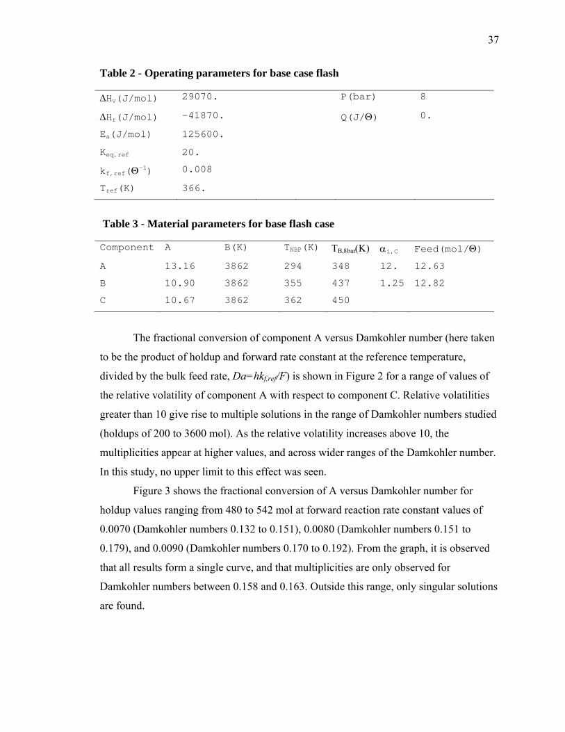
37

Table 2 - Operating parameters for base case flash

Table 3 - Material parameters for base flash case

Component A B(K) TNBP(K) ΤΒ,8bar(Κ) αi,C Feed(mol/Θ)

A 13.16 3862 294 348 12. 12.63

B 10.90 3862 355 437 1.25 12.82

C 10.67 3862 362 450

The fractional conversion of component A versus Damkohler number (here taken

to be the product of holdup and forward rate constant at the reference temperature,

divided by the bulk feed rate, Da=hkf,ref/F) is shown in Figure 2 for a range of values of

the relative volatility of component A with respect to component C. Relative volatilities

greater than 10 give rise to multiple solutions in the range of Damkohler numbers studied

(holdups of 200 to 3600 mol). As the relative volatility increases above 10, the

multiplicities appear at higher values, and across wider ranges of the Damkohler number.

In this study, no upper limit to this effect was seen.

Figure 3 shows the fractional conversion of A versus Damkohler number for

holdup values ranging from 480 to 542 mol at forward reaction rate constant values of

0.0070 (Damkohler numbers 0.132 to 0.151), 0.0080 (Damkohler numbers 0.151 to

0.179), and 0.0090 (Damkohler numbers 0.170 to 0.192). From the graph, it is observed

that all results form a single curve, and that multiplicities are only observed for

Damkohler numbers between 0.158 and 0.163. Outside this range, only singular solutions

are found.

∆Hv(J/mol) 29070. P(bar) 8

∆Hr(J/mol) -41870. Q(J/Θ) 0.

Ea(J/mol) 125600.

Keq,ref 20.

kf,ref(Θ-1) 0.008

Tref(K) 366.

38

0

0.1

0.2

0.3

0.4

0.5

0 0.2 0.4 0.6 0.8 1 1.2

Dam kohler num ber

Spec

ies

A C

onve

rsio

n

alph

a =

10

alph

a =

12

alph

a =

14

alph

a =

18

alph

a =

22

Figure 2 - Conversion versus Damkohler number for a range of species A relative volatilities

0.10

0.15

0.20

0.25

0.30

0.35

0.40

0.125 0.135 0.145 0.155 0.165 0.175 0.185 0.195

Damkohler number

Frac

tiona

l con

vers

ion

of A

Figure 3 - Conversion versus Damkohler number for a range of rate constant values

39

Conversion versus Damkohler number for a range of reaction equilibrium

constant values is shown in Figure 4. It can be seen that as the value of the chemical

equilibrium constant increases, the range of Damkohler number for which multiplicities

are observed grows wider and moves toward smaller values of the Damkohler number.

For values of the equilibrium constant below about 15, singular solutions are obtained,

and multiplicities are no longer found. For a reference temperature equilibrium constant

of 18, multiplicities are found in a range of Damkohler numbers from about 0.162 to

0.165; when the equilibrium constant is 22, the range of Damkohler numbers is from

about 0.154 to 0.162.

0.15

0.2

0.25

0.3

0.35

0.4

0.151 0.156 0.161 0.166

Damkohler number

Frac

tiona

l con

vers

ion

of A K=22

K=20K=18

K=15

K=25

0.170

Figure 4 - Conversion versus Damkohler number for a range of equilibrium constant values

3. THE REACTIVE COLUMN

Figure 5 represents a multistage column in which a reaction A+B ↔ C takes place

in the liquid phase on designated trays. Nonreactive trays are specified by setting the

holdup to zero for those stages. Since the single product C is the heavy component, and is

ideally the only species leaving the column, non-reacting stages are placed at the column

40

bottom to return components A and B to the reactive section at the top. The heavier of the

two reactants is fed at the top of the reactive section, while the lighter component is fed to

the lowest reactive stage. Modeling the column’s performance is accomplished in the

same way as for the flash, except that the equation set to be solved consists of the eight

material balance, energy balance, equilibrium, and reaction extent equations for each

stage, or a total of 8n equations:

lA,j +vA,j –fA,j –lA,j-1 –vA,j+1 - hλjυΑ = 0

lB,j +vB,j –fB,j –lB,j-1 –vB,j+1 - hλjυΒ = 0

lC,j +vC,j –fC,j –lC,j-1 –vC,j+1 - hλjυC = 0

HVj +HLj –HFj – HLj-1 –HVj+1 -Qj = 0

KAjlAj/Lj –vAj/Vj = 0

KBjlBj/Lj –vBj/Vj = 0

KCjlCj/Lj –vCj/Vj = 0

hjkf[(l’Aj/Lj’)(l’Bj/Lj’) – (1/Ke)(l’Cj/Lj’)] - λj = 0

Tables 4 and 5 contain the parameters for the column base case. The heat of

reaction is -41,870 J/mol, activation energy 125,600 J/mol, reaction equilibrium constant

20, and forward rate constant 0.008 per unit of time at a reference temperature of 366 K.

Component normal boiling points are 313 K. 338 K, and 353 K for A, B, and C

respectively. These parameters are substantially the same as those describing the case

presented by Luyben and Yu (2008), and except for the observation of solution

multiplicities, comparable results were obtained.

41

Figure 5 - Reactive column

Table 4 - Operating parameters for base distillation case

Table 5 - Component parameters for base distillation case

Component A B(K) TNBP(K) TB,8bar(K) αi,C Feed(mol/Θ)

A 12.34 3862 313 376 4. 12.63

B 11.45 3862 338 412 1.6 12.82

C 10.96 3862 353 435

∆Hv(J/mol) 29070. stages 16

∆Hr(J/mol) -41870. react stages

2-10

Ea(J/mol) 125600. Β feed stage 2

Keq,ref 20. A feed stage 10

kf,ref(Θ-1) 0.008 Condenser Total

Tref(K) 366. P(bar) 8

L16(mol/Θ) 12.85

V16(mol/Θ) 62.03

B feed

A feed

Condenser stage 1

Reboiler stage 16

10

QR

QC

V1

L16

2

42

Figure 6 shows the fractional conversion of A versus distillate-to-total-feed ratio

(D/F) at various levels of the relative volatility spread between components A and C. For

relative volatilities at or below 3.4, and in all cases for D/F less than about 0.016, singular

solutions are obtained and multiplicities are not observed. For a relative volatility of 3.8,

multiplicities are found for D/F in the range of about 0.019 to 0.022, and as the relative

volatility increases, the range of D/F for which multiplicities are observed becomes wider

and reaches higher D/F values. In the range of conditions studied, conversions as high as

97 percent were found where multiplicities existed. However, for a relative volatility

spread of 3.4, singular solutions were found and maximum conversion was only 95.6

percent.

Figure 7 demonstrates the effect of varying the reference forward rate constant

kf,ref on the relationship between conversion and D/F. As with the relative volatility

spread, multiplicities are not observed for D/F less than about 0.014. In the range of

values studied, smaller forward rate constants result in higher values and broader ranges

of D/F for which multiple solutions are obtained.

The variation in conversion with D/F for several values of the reaction

equilibrium constant Ke is shown in Figure 8. For values of Ke at or below 10, multiple

solutions are not observed in the range of D/F studied. For values of Ke of 15 and above,

increasing Ke leads to narrower ranges and lower values of D/F where multiple solutions

are to be found.

4. CONCLUSIONS

The occurrence of steady-state multiplicities for both the single stage reactive

flash and the multistage reactive column is influenced by both the vapor-liquid and

reaction kinetic properties of the components involved. For the idealized ternary system

studied, this has been examined in terms of the relative volatility between the lightest and

heaviest components, and forward rate constant and equilibrium constant for the reaction.

The occurrence of multiplicities appears to be caused by interaction between the relative

rates of component evaporation which do not change sign, and the rates of production or

consumption which can change sign.

43

0.91

0.92

0.93

0.94

0.95

0.96

0.97

0.98

0.000 0.005 0.010 0.015 0.020 0.025 0.030 0.035 0.040

D/F

Con

vers

ion

of A

Alpha = 4.6

Alpha = 4.2

Alpha = 3.8Alpha = 3.4

Figure 6 - Conversion versus distillate to feed ratio for a range of relative volatilities

0.89

0.90

0.91

0.92

0.93

0.94

0.95

0.96

0.97

0.98

0.000 0.005 0.010 0.015 0.020 0.025 0.030 0.035 0.040

D/F

Con

vers

ion

of A

k = 0.006

k = 0.020

k = 0.004

k = 0.008

Figure 7 - Conversion versus distillate to feed ratio for a range of values of the forward rate constant

44

0.82

0.84

0.86

0.88

0.90

0.92

0.94

0.96

0.98

1.00

0.000 0.005 0.010 0.015 0.020 0.025 0.030 0.035 0.040D/F

Con

vers

ion

of A

Ke = 30

Ke = 15

Ke = 10

Ke = 25

Ke = 20

Figure 8 - Conversion versus distillate to feed ratio for a range of values of the reaction equilibrium constant

Multiplicities are observed only for values of the relative volatility spread above

some minimum value, below which only singular solutions are found. As the relative

volatility difference increases above the minimum, multiplicities are observed at

increasing valuesof the Damkohler number in the case of the flash, and distillate to feed

ratio in the case of the column. This could be accounted for by the greater tendency of the

light reactant to leave the system rather than reacting as relative volatility increases.

In the flash, multiplicities appear to exist only for values of the Damkohler

number between about 0.158 and 0.163, throughout the range of rate constant values

studied. This can be attributed to the fact that higher rate constant and lower holdup have

a tendency to offset each other in determining reaction extent. For the column, singular

solutions are observed for distillate to feed ratio less than about 0.014. Above this

threshold, increasing rate constant values correspond to the appearance of multiplicities at

lower values and narrower ranges of distillate to feed ratio.

For the column, under the conditions studied, conversion was limited to 95.6

percent when the relative volatility was in a range where singular solutions were found.

45

Higher conversions were observed; however, they occurred in regions where solution

multiplicities were encountered. For each of the three properties studied, the downward

slope of the curves representing high conversion solutions indicates a limit imposed by

removal of reactants in the overhead, rather than attainment of reaction equilibrium.

For both the flash and the column, there appears to be a threshold value of the

equilibrium constant below which multiplicities are not exhibited. Above that threshold,

multiplicities are found at lower values of the Damkohler number in the flash and

distillate to feed ratio in the column, as the equilibrium constant increases.

NOMENCLATURE




Fj molar bulk feed rate, mol/time

fij component i feed rate, mol/time







Ke,0 reaction equilibrium constant pre-exponential




P*i component i vapor pressure, bar

P pressure, bar


R gas constant

rj rate of reaction, moles per unit time

Tj temperature, K


46




Greek letters

αi component i relative volatility



υi component i stoichiometric coefficient

Θ unit of time

Subscripts

i component index

j stage index

l liquid phase

v vapor phase

REFERENCES


Bessling, B, G Schembecker, and K H Simmrock. 1997. Design of Processes with Reactive Distillation Line Diagrams. Ind. Eng. Chem. Res. 36: 3032-3042

Choi, Soo Hyoung. 1990. The Application of Global Homotopy Continuation Methods to Chemical Process Flowsheeting Problems. PhD diss., University of Missouri - Rolla.

Choi, Soo Hyoung, David Anthony Harney, and Neil L Book. 1996. A Robust Path Tracking Algorithm for Homotopy Continuation. Computers and Chemical Engineering 20: 647-655. Dalal, Nirav M, and Ranjan K Malik. 2003. Solution Multiplicity in Multicomponent Distillation a Computational Study. Computer-Aided Chemical Engineering 14 (European Symposium on Computer Aided Process Engineering--13, 2003): 617-622.



47



Singh, B P, R Singh, M V P Kumar, and N Kaistha. 2005. Steady State Analysis of Reactive Distillation Using Homotopy Continuation. Chemical Engineering Research and Design 83(A8): 959-968.


48

SECTION

3. CONCLUSIONS

Output multiplicities are found for both the reactive flash and the multistage

reactive distillation, even for systems described by highly idealized models. Multiplicities

in these ideal systems are seen to be caused by interaction between components’ relative

rates of evaporation which cannot change sign, and rates of production or consumption

which can change sign. Homotopy continuation is found to be a useful tool for

identifying these multiplicities, and for locating regions in parameter space where they

occur.

The occurrence of multiplicities for both the single stage reactive flash and the

multistage reactive column is influenced by both the vapor-liquid and reaction kinetic

properties of the components involved. For the idealized ternary system studied, this has

been looked at in terms of the relative volatility between the lightest and heaviest

components, and the reaction forward rate constant and equilibrium constant.

Multiplicities are observed only for values of the relative volatility spread above

some minimum value; below this value, only singular solutions are found. As the relative

volatility difference increases above the minimum, multiplicities are observed at

increasing values of Damkohler number in the case of the flash, and distillate to feed ratio

in the case of the column.

In the flash, multiplicities appear to exist only for values of Damkohler number

between about 0.158 and 0.163, throughout the range of rate constant values studied. For

the column, singular solutions are observed for distillate to feed ratio less than about

0.016. Above this threshold, increasing rate constant values correspond to the appearance

of multiplicities at lower values and narrower ranges of distillate to feed ratio.

For both the flash and the column, there appears to be a threshold value of the

equilibrium constant below which multiplicities are not exhibited. Above that threshold,

multiplicities are found at lower values of Damkohler number in the flash and distillate to

feed ratio in the column, as the equilibrium constant increases.

49

The choice of specifications, or by extension the choice of control variables in the

physical operation, also affects the occurrence of these multiplicities. In the reactive

flash, specifying the heat input can give rise to multiplicities, while specifying the

fraction of the feed vaporized does not. For the column, specifying the boilup and the

bottoms rate - one being an internal energy balance variable, and the other an external

material balance variable - fails to produce multiplicities. In contrast, specifying both the

boilup and the reflux rate - both internal energy balance variables - can give rise to

multiple solutions. For both the flash and the column, when other specifications are

favorable for the existence of multiplicities, they are exhibited for some ranges of

Damkohler number values (as determined by holdup), but not for other values.

50

APPENDIX A.

COMPUTER PROGRAMS USED FOR THIS STUDY

51

The computer programs used in this study were coded in the FORTRAN 77

language, and compiled using the MINGW g77 compiler. The distillation program was

prepared initially, and was then modified to create the flash program by removing the

logic needed for unique handling of a condenser, reboiler, and multiple stages. Each

program consists of routines for receiving problem specifications, constructing the vector

of initial estimates, calling the solver routine, monitoring the state returned by the solver,

and printing formatted results. The homotopy solver routine for both programs is as

published by Choi (1990).

PROGRAM INPUT

Input to both the distillation and flash programs is through text files containing a

series of “command” lines describing a case or series of cases to be run. For the

distillation program, the input formats are presented in Table A.1. Table A.2 contains the

input formats for the flash program, which differ from those for the distillation program

only in that a single stage, rather than multiple stages, is specified for each case.

Table A.1

Distillation Program Input file "card" format and content

Case Identification string (Required)

P1 <string>

Case Description

P2 <string>

Case solution algorithm (Default: Newton)

P3 <integer>

1 => Newton solver (default)

2 => Homotopy solver

Thermodynamic model (Ideal only for current thermodynamic subroutines)

P4 <integer>

1=> Peng-Robinson EOS (default)

2=> Soave-Redlich-Kwong EOS

3=> Redlich-Kwong EOS

4=> Van der Waals EOS

52

Table A.1 (cont.)

Component specifications (Required)

P5 <no. components> <"datafile name">

<"component name">

...

<"component name">

Number of stages (incl. condenser and reboiler) (Required)

P6 <integer>

Condenser type (Default: Total)

P7 <integer>

1 => Total (default)

2 => Partial

Top specification (Required)

P8 <spec type> <spec value> <component index>

1=> Qc (J)

2=> L/D

3=> D/F

4=> Di/Fi

5=> Tc (K)

11=> L1 (mol)

Bottom specification (Required)


6=> Tr (K)

7=> Bi/Fi

8=> B/F

9=> V/B

10=> Qr (J)

12=> Vn (mol)

Condenser pressure and per-stage delta (Required)

P10 <Pcond> <delta>

Feed specifications (Required)

P11 <no. feeds>

<stage> <type> <pressure> <temperature> <feed 1> ... <feed nc>

...

<stage> <type> <pressure> <temperature>

1=> Bubble point liquid (temperature is recalculated)

53

Table A.1 (cont.)

2=> Dew point vapor (temperature is recalculated)

3=> Feed flashed at spec. temperature and stage pressure

Specified stage heat duties (Default: 0.0 for all stages)

P12 <Start stage> <End stage> <specified input(+) or withdrawal(-)>

Specified side-draws (Default: 0.0 for all stages)

P13 <no. specified>

<stage> <type> <specified Sv/V or Sl/L>

...

<stage> <type> <specified Sv/V or Sl/L>

1=> liquid

2=> vapor

note that both liquid and vapor side-draws can

be specified for each stage

Specified Murphree (VLE) efficiencies (Default: 1.0 for all stages)

P14 <Start stage> <End stage> <specified efficiency>

Specified stoichiometric coefficients (Default: 0.0 for all comps)

P15 <c1> <c2> ... <cn>

(+)=> reagent

(-)=> product

(0)=> inert

Specified stage reaction efficiencies (Default: 0.0 for all stages)

P16 <Start stage> <End stage> <specified efficiency>

Specified reaction equilibrium constant (Default 0.0)

P17 <spec. value>

note that if the specified value is zero, program will use

the value calculated from the thermodynamic model

Specified stage molar holdups (Default: 0.0 for all stages)

P18 <Start stage> <End stage> <specified holdup>

Specified homotopy solver parameters

P21 <param number> <value>

1) dir tracking direction (default = 1 [positive t]; -1 for negative t)

2) dso initial step size (default = 1.0d-01)

3) dsmin minimum step size (default = 1.0d-20)

54

Table A.1 (cont.)

4) dsmax maximum step size (default = 5.0d+04)

5) xmax continuation space boundary (default = 1.0d+05)

6) ecorc continuation point tolerance (default = 1.0d-04)

7) ecorb bisection point tolerance (default = 1.0d-06)

8) edet max relative determinant change (default = 5.0d-01)

9) esol solution point tolerance (default = 1.0d-04)

10) ebif bifurcation point tolerance (default = 1.0d-04)

11) etur turn point tolerance (default = 1.0d-06)

12) esta start point tolerance (default = 1.0d-04)

13) easy asymtotic behavior tolerance (default = 1.0d-06)

14) idom compute in real or complex domain (default = 0 [real domain])

15) ihom homotopy type (default = 1 [newton]; 2 for fixed point)

16) maxdet maximum number of determinant evaluations (default = 5)

17) minasy minimum steps to sense asymtote (default = 5)

18) maxasy maximum steps to sense asymtote (default = 20)

Parameters for simplified thermodynamic calculations

P31 <alpha> <tb1> <delhv> <delhr> <cpl> <cpv> <rxntref> <rxnk> <rxnkf> <rxefwd>

alpha Component to component relative volatility

tb1 Boiling point of lightest component

delhv Heat of vaporization (same for all components)

delhr Heat of reaction

cpl Liquid heat capacity (same for all components)

cpv Vapor heat capacity (same for all components)

rxntref Reference Temperature for reaction equilibrium and rate constants

rxnk Reaction equilibrium constant at rxntref

rxkf Reaction forward rate constant at rxntref

rxefwd Activation energy (for forward rate constant)

Parameters for specified Antoine constants (ln P = A - B/T)

P32 <Component index> <A> <B>

Reaction coordinate for problem initialization

P33 <rx coord> ( 0 <= rxcoord <= 1 )

0<=rxcoord<=1 initialization reaction coordinate

rxcoord>1 or <-1 initialization at full equilibrium

0>rxcoord>-1 initialize at fract approach to equilibrium

55

Table A.1 (cont.)

Component flow scaling for problem initialization

P34 <scinit>

Multiply component flows by scinit for starting vector

End of current case

XC

Table A.2

Input file "card" format and content for flash program

Case Identification string (Required)

P1 <string>

Case Description

P2 <string>

Case solution algorithm (Default: Newton)

P3 <integer>

1 => Newton solver (default)

2 => Homotopy solver

Thermodynamic model (Ideal only for current thermodynamic subroutines)

P4 <integer>

1=> Peng-Robinson EOS (default)

2=> Soave-Redlich-Kwong EOS

3=> Redlich-Kwong EOS

4=> Van der Waals EOS

Component specifications (Required)

P5 <no. components> <"datafile name">

<"component name">

...

<"component name">

Number of stages (incl. condenser and reboiler) (Required)

P6 <integer>

56

Table A.2 (cont.)

Condenser type (Default: Total)

P7 <integer>

1 => Total (default)

2 => Partial

Top specification (Required)


1=> Spec V/F

2=> Spec T

3=> Spec Q

Flash pressure and per-stage delta (Required)

P10 <Pflash>

Feed specifications (Required)

P11 <no. feeds>

<stage> <type> <pressure> <temperature> <feed 1> ... <feed nc>

...

<stage> <type> <pressure> <temperature>

1=> Bubble point liquid (temperature is recalculated)

2=> Dew point vapor (temperature is recalculated)

3=> Feed flashed at spec. temperature and stage pressure

Specified stoichiometric coefficients (Default: 0.0 for all comps)

P15 <c1> <c2> ... <cn>

(+)=> reagent

(-)=> product

(0)=> inert

Specified stage reaction efficiencies (Default: 0.0 for all stages)

P16 <specified efficiency>

Specified stage molar holdups (Default: 0.0 for all stages)

P18 <specified holdup>

Specified homotopy solver parameters

P21 <param number> <value>

1) dir tracking direction (default = 1 [positive t]; -1 for negative t)

2) dso initial step size (default = 1.0d-01)

3) dsmin minimum step size (default = 1.0d-20)

4) dsmax maximum step size (default = 5.0d+04)

5) xmax continuation space boundary (default = 1.0d+05)

57

Table A.2 (cont.)

6) ecorc continuation point tolerance (default = 1.0d-04)

7) ecorb bisection point tolerance (default = 1.0d-06)

8) edet max relative determinant change (default = 5.0d-01)

9) esol solution point tolerance (default = 1.0d-04)

10) ebif bifurcation point tolerance (default = 1.0d-04)

11) etur turn point tolerance (default = 1.0d-06)

12) esta start point tolerance (default = 1.0d-04)

13) easy asymtotic behavior tolerance (default = 1.0d-06)

14) idom compute in real or complex domain (default = 0 [real domain])

15) ihom homotopy type (default = 1 [newton homotopy])

16) maxdet maximum number of determinant evaluations (default = 5)

17) minasy minimum steps to sense asymtote (default = 5)

18) maxasy maximum steps to sense asymtote (default = 20)

Parameters for simplified thermodynamic calculations

P31 <alpha> <tb1> <delhv> <delhr> <cpl> <cpv> <rxntref> <rxnk> <rxnkf> <rxefwd>

alpha Component to component relative volatility

tb1 Boiling point of lightest component

delhv Heat of vaporization (same for all components)

delhr Heat of reaction

cpl Liquid heat capacity (same for all components)

cpv Vapor heat capacity (same for all components)

rxntref Reference Temperature for reaction equilibrium and rate constants

rxnk Reaction equilibrium constant at rxntref

rxkf Reaction forward rate constant at rxntref

rxefwd Activation energy (for forward rate constant)

Parameters for specified Antoine constants (ln P = A - B/T)

P32 <Component index> <A> <B>

Reaction coordinate for problem initialization

P33 <rx coord> ( 0 <= rxcoord <= 1 )

( rxcoord >1 or <=-1 full equil)

(-1<rxcoord<0 partial equil)

Initialization scale factor

P34 <scinit>

End of current case

XC

58

PARAMETERS FOR THE HOMOTOPY SOLVER

Originally, Choi’s path tracking algorithm was presented with a set of default

parameters suitable for problems having two- or three-dimensional solution vectors. For

the distillation problems involved in this study, solution vectors are commonly in excess

of 100-dimensional. To obtain solutions to these larger problems in a reasonable number

of steps, it was found necessary to increase the default initial step size, as shown in Table

A.3. For some specific problems, it was also found useful to increase the minimum step

size and to tighten the tolerance for identifying continuation points.

Table A.3

Parameter Description Choi value Value used

dir Tracking direction 1 (t incr.)

dso Initial step size 1.0d-02 1.0d-01

dsmin Minimum step size 1.0d-20 1.0d-20

dsmax Maximum step size 5.0d+04 5.0d+04

xmax Continuation space boundary 1.0d+05 1.0d+05

ecorc Continuation point tolerance 1.0d-04 1.0d-04

ecorb Bisection point tolerance 1.0d-06 1.0d-06

edet Maximum relative determinant change 5.0d-01 5.0d-01

esol Solution point tolerance 1.0d-04 1.0d-04

ebif Bifurcation point tolerance 1.0d-04 1.0d-04

etur Turn point tolerance 1.0d-06 1.0d-06

esta Start point tolerance 1.0d-04 1.0d-04

easy Asymptotic behavior tolerance 1.0d-06 1.0d-06

idom Compute in real or complex domain 0 (real)

ihom Homotopy type 1 (Newton)

maxdet Maximum determinant evaluations 5 5

minasy Minimum steps to sense asymptote 5 5

maxasy Maximum steps to sense asymptote 20 20

59

PROGRAM USE AND VALIDATION

Table A.4 shows the program input for an example problem corresponding to the

ternary case described by Luyben and Yu (2008). In this example, the light component,

A, is fed to stage 10, and the intermediate boiling component, B, is fed to stage 2 of a

column totaling 16 stages, including a total condenser. Reflux is specified at 78.5 moles

per time unit, and boilup is 62.03 moles. Stages 11 through 16 and the condenser (stage

1) are specified to have no liquid holdup, and are thus nonreacting. On stages 2 through

10, holdup is specified at 1000 moles, and the reaction of A and B to form C proceeds.

Table A.4

P1 EX-001

P2 "Multiple Soln Example Case h=1000"

P3 2

P5 3 "scomps.dat"

"A"

"B"

"C"

P6 16

P7 1

P8 11 78.50 0

P9 12 62.03 0

P10 8.000 0.

P11 2

2 1 8.000 0. 0. 12.82 0.

10 1 8.000 0. 12.63 0. 0.

P15 -1. -1. 1.

P18 1 16 0.0

P18 2 10 1000.

P21 1 1.

P21 3 1.d-06

P21 6 1.d-06

P21 10 0.

P21 13 1.d-04

P31 2.0 352 29070. -41870. 0. 0. 366. 20.0 0.008 125600.

P32 1 12.34 3862.

P32 2 11.45 3862.

P32 3 10.96 3862.

XC

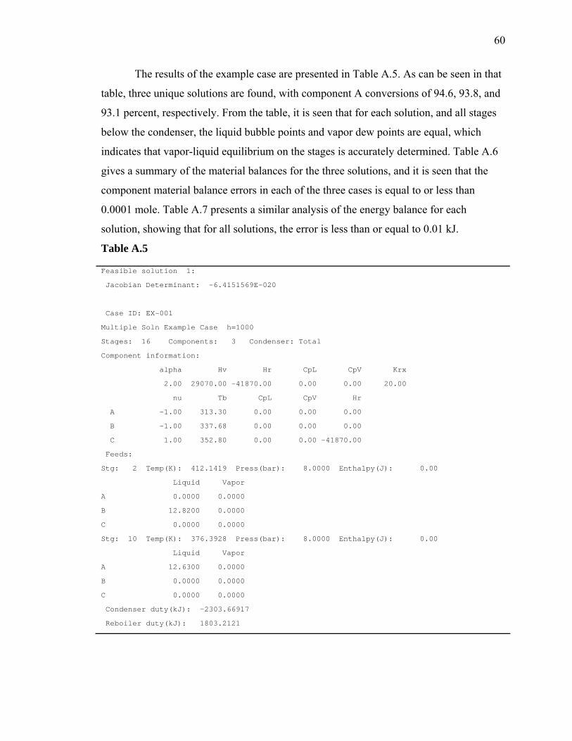
60

The results of the example case are presented in Table A.5. As can be seen in that

table, three unique solutions are found, with component A conversions of 94.6, 93.8, and

93.1 percent, respectively. From the table, it is seen that for each solution, and all stages

below the condenser, the liquid bubble points and vapor dew points are equal, which

indicates that vapor-liquid equilibrium on the stages is accurately determined. Table A.6

gives a summary of the material balances for the three solutions, and it is seen that the

component material balance errors in each of the three cases is equal to or less than

0.0001 mole. Table A.7 presents a similar analysis of the energy balance for each

solution, showing that for all solutions, the error is less than or equal to 0.01 kJ.

Table A.5

Feasible solution 1:

Jacobian Determinant: -6.4151569E-020

Case ID: EX-001

Multiple Soln Example Case h=1000

Stages: 16 Components: 3 Condenser: Total

Component information:

alpha Hv Hr CpL CpV Krx

2.00 29070.00 -41870.00 0.00 0.00 20.00

nu Tb CpL CpV Hr

A -1.00 313.30 0.00 0.00 0.00

B -1.00 337.68 0.00 0.00 0.00

C 1.00 352.80 0.00 0.00 -41870.00

Feeds:

Stg: 2 Temp(K): 412.1419 Press(bar): 8.0000 Enthalpy(J): 0.00

Liquid Vapor

A 0.0000 0.0000

B 12.8200 0.0000

C 0.0000 0.0000


Liquid Vapor

A 12.6300 0.0000

B 0.0000 0.0000

C 0.0000 0.0000

Condenser duty(kJ): -2303.66917

Reboiler duty(kJ): 1803.2121

61

Table A.5 (cont.)

Column profiles:

Stg Q(kJ) L s/d V s/d VLE eff Rxn eff Rx(mol) Rx(kJ)

1 0.0000 0.0000 0.0000 1.0000 0.0000 0.0000 0.0000

2 0.0000 0.0000 0.0000 1.0000 0.0000 0.0000 0.0000

3 0.0000 0.0000 0.0000 1.0000 0.0000 0.0000 0.0000

4 0.0000 0.0000 0.0000 1.0000 0.0000 0.0000 0.0000

5 0.0000 0.0000 0.0000 1.0000 0.0000 0.0000 0.0000

6 0.0000 0.0000 0.0000 1.0000 0.0000 0.0000 0.0000

7 0.0000 0.0000 0.0000 1.0000 0.0000 0.0000 0.0000

8 0.0000 0.0000 0.0000 1.0000 0.0000 0.0000 0.0000

9 0.0000 0.0000 0.0000 1.0000 0.0000 0.0000 0.0000

10 0.0000 0.0000 0.0000 1.0000 0.0000 0.0000 0.0000

11 0.0000 0.0000 0.0000 1.0000 0.0000 0.0000 0.0000

12 0.0000 0.0000 0.0000 1.0000 0.0000 0.0000 0.0000

13 0.0000 0.0000 0.0000 1.0000 0.0000 0.0000 0.0000

14 0.0000 0.0000 0.0000 1.0000 0.0000 0.0000 0.0000

15 0.0000 0.0000 0.0000 1.0000 0.0000 0.0000 0.0000

16 0.0000 0.0000 0.0000 1.0000 0.0000 0.0000 0.0000

Stg P(bar) T(K) L(mol) V(mol) H err L(kJ) V(kJ)

1 8.0000 379.0299 78.5000 0.7456 0.0000 -116.6714 -1.1081

-1.4863 -1.4863

2 8.0000 383.4764 79.0314 79.2456 0.0000 -386.2836 2185.8897

-4.8877 27.5837

3 8.0000 384.7029 71.2751 71.9926 0.0000 -556.6481 1916.2774

-7.8099 26.6177

4 8.0000 385.6978 66.9209 67.4147 0.0000 -658.7248 1745.9129

-9.8433 25.8981

5 8.0000 386.6226 64.5933 64.8448 0.0000 -727.9711 1643.8363

-11.2701 25.3503

6 8.0000 387.7843 63.2327 63.4711 0.0000 -792.4642 1574.5899

-12.5325 24.8080

7 8.0000 389.5321 62.1564 62.6680 0.0000 -869.2428 1510.0969

-13.9848 24.0968

8 8.0000 392.1110 61.0314 62.0328 0.0000 -958.9623 1433.3183

-15.7126 23.1058

9 8.0000 395.4112 60.1642 61.3687 0.0000 -1047.6754 1343.5988

-17.4136 21.8939

10 8.0000 399.0068 74.7818 60.8569 0.0000 -1404.1432 1254.8856

-18.7765 20.6203

11 8.0000 410.1494 74.7818 62.0300 0.0000 -1863.4536 898.4179

-24.9186 14.4836

62

Table A.5 (cont.)

12 8.0000 420.1300 74.7818 62.0300 0.0000 -2246.3074 439.1075

-30.0382 7.0790

13 8.0000 426.4226 74.7818 62.0300 0.0000 -2511.8416 56.2537

-33.5890 0.9069

14 8.0000 429.7994 74.7818 62.0300 0.0000 -2694.8914 -209.2806

-36.0367 -3.3739

15 8.0000 431.6652 74.7818 62.0300 0.0000 -2828.0138 -392.3303

-37.8169 -6.3248

16 8.0000 432.8257 12.7518 62.0300 0.0000 -499.3489 -525.4528

-39.1592 -8.4709

Vapor flows/compositions:

A B C

1 0.6656 0.0536 0.0265

0.892671 0.071832 0.035497

2 70.7403 5.6923 2.8130

0.892671 0.071832 0.035497

3 64.0695 3.7065 4.2166

0.889946 0.051485 0.058570

4 59.7006 2.6071 5.1071

0.885571 0.038673 0.075756

5 56.9320 2.1521 5.7607

0.877973 0.033188 0.088839

6 54.8454 2.1648 6.4608

0.864101 0.034107 0.101791

7 52.5960 2.6284 7.4436

0.839280 0.041942 0.118778

8 49.5212 3.6753 8.8363

0.798307 0.059248 0.142445

9 45.3693 5.4814 10.5180

0.739290 0.089319 0.171391

10 40.5861 7.9894 12.2815

0.666910 0.131281 0.201809

11 27.8693 12.5511 21.6096

0.449287 0.202339 0.348373

12 14.4282 15.0222 32.5795

0.232601 0.242177 0.525222

13 5.9655 14.3411 41.7234

0.096172 0.231196 0.672632

14 2.1461 11.8186 48.0653

0.034598 0.190531 0.774871

15 0.7112 8.8817 52.4371

63

Table A.5 (cont.)

0.011465 0.143184 0.845351

16 0.2187 6.1948 55.6165

0.003525 0.099868 0.896607

Liquid flows/compositions:

A B C

1 70.0747 5.6388 2.7865

0.892671 0.071832 0.035497

2 58.3683 11.4373 9.2258

0.738546 0.144719 0.116736

3 50.8209 7.1595 13.2947

0.713025 0.100448 0.186526

4 46.2681 4.9202 15.7326

0.691385 0.073523 0.235093

5 43.2277 3.9791 17.3865

0.669229 0.061603 0.269168

6 40.4208 3.8852 18.9268

0.639238 0.061443 0.299319

7 36.9049 4.4910 20.7605

0.593742 0.072254 0.334004

8 32.2920 5.8361 22.9033

0.529105 0.095624 0.375271

9 27.1534 7.9887 25.0221

0.451322 0.132781 0.415897

10 27.8811 13.3649 33.5358

0.372833 0.178719 0.448449

11 14.4400 15.8360 44.5057

0.193096 0.211763 0.595141

12 5.9773 15.1549 53.6496

0.079930 0.202654 0.717415

13 2.1579 12.6324 59.9914

0.028856 0.168924 0.802220

14 0.7230 9.6955 64.3633

0.009668 0.129650 0.860682

15 0.2305 7.0086 67.5427

0.003082 0.093721 0.903198

16 0.0118 0.8138 11.9262

0.000925 0.063819 0.935256

Component creation & consumption:

A B C

1 0.0000 0.0000 0.0000

2 -5.0357 -5.0357 5.0357

64

Table A.5 (cont.)

3 -3.1784 -3.1784 3.1784

4 -1.7843 -1.7843 1.7843

5 -0.9538 -0.9538 0.9538

6 -0.5576 -0.5576 0.5576

7 -0.4410 -0.4410 0.4410

8 -0.4610 -0.4610 0.4610

9 -0.3554 -0.3554 0.3554

10 0.8145 0.8145 -0.8145

11 0.0000 0.0000 0.0000

12 0.0000 0.0000 0.0000

13 0.0000 0.0000 0.0000

14 0.0000 0.0000 0.0000

15 0.0000 0.0000 0.0000

16 0.0000 0.0000 0.0000

Vapor/Liquid equilibrium ratios:

A B C

1 0.1074E+01 0.4410E+00 0.2702E+00

0.1000E+01 0.1000E+01 0.1000E+01

2 0.1209E+01 0.4964E+00 0.3041E+00

0.1209E+01 0.4964E+00 0.3041E+00

3 0.1248E+01 0.5126E+00 0.3140E+00

0.1248E+01 0.5126E+00 0.3140E+00

4 0.1281E+01 0.5260E+00 0.3222E+00

0.1281E+01 0.5260E+00 0.3222E+00

5 0.1312E+01 0.5387E+00 0.3301E+00

0.1312E+01 0.5387E+00 0.3301E+00

6 0.1352E+01 0.5551E+00 0.3401E+00

0.1352E+01 0.5551E+00 0.3401E+00

7 0.1414E+01 0.5805E+00 0.3556E+00

0.1414E+01 0.5805E+00 0.3556E+00

8 0.1509E+01 0.6196E+00 0.3796E+00

0.1509E+01 0.6196E+00 0.3796E+00

9 0.1638E+01 0.6727E+00 0.4121E+00

0.1638E+01 0.6727E+00 0.4121E+00

10 0.1789E+01 0.7346E+00 0.4500E+00

0.1789E+01 0.7346E+00 0.4500E+00

11 0.2327E+01 0.9555E+00 0.5854E+00

0.2327E+01 0.9555E+00 0.5854E+00

12 0.2910E+01 0.1195E+01 0.7321E+00

0.2910E+01 0.1195E+01 0.7321E+00

13 0.3333E+01 0.1369E+01 0.8385E+00

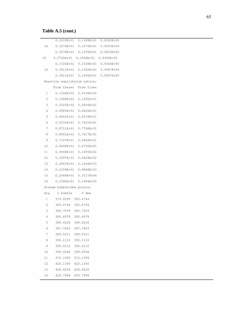
65

Table A.5 (cont.)

0.3333E+01 0.1369E+01 0.8385E+00

14 0.3579E+01 0.1470E+01 0.9003E+00

0.3579E+01 0.1470E+01 0.9003E+00

15 0.3720E+01 0.1528E+01 0.9360E+00

0.3720E+01 0.1528E+01 0.9360E+00

16 0.3811E+01 0.1565E+01 0.9587E+00

0.3811E+01 0.1565E+01 0.9587E+00

Reaction equilibrium ratios:

From thermo From flows

1 0.1246E+02 0.5536E+00

2 0.1068E+02 0.1092E+01

3 0.1025E+02 0.2604E+01

4 0.9905E+01 0.4625E+01

5 0.9601E+01 0.6529E+01

6 0.9233E+01 0.7621E+01

7 0.8711E+01 0.7786E+01

8 0.8001E+01 0.7417E+01

9 0.7187E+01 0.6940E+01

10 0.6408E+01 0.6730E+01

11 0.4548E+01 0.1455E+02

12 0.3397E+01 0.4429E+02

13 0.2847E+01 0.1646E+03

14 0.2594E+01 0.6866E+03

15 0.2466E+01 0.3127E+04

16 0.2390E+01 0.1584E+05

Stream bubble/dew points:

Stg L bubble V dew

1 379.0299 383.4764

2 383.4764 383.4764

3 384.7029 384.7029

4 385.6978 385.6978

5 386.6226 386.6226

6 387.7843 387.7843

7 389.5321 389.5321

8 392.1110 392.1110

9 395.4112 395.4112

10 399.0068 399.0068

11 410.1494 410.1494

12 420.1300 420.1300

13 426.4226 426.4226

14 429.7994 429.7994

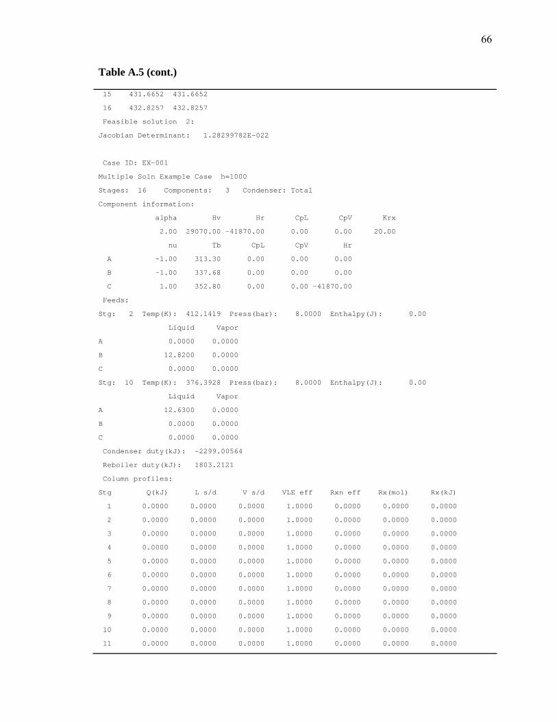
66

Table A.5 (cont.)

15 431.6652 431.6652

16 432.8257 432.8257


Jacobian Determinant: 1.28299782E-022

Case ID: EX-001





2.00 29070.00 -41870.00 0.00 0.00 20.00

nu Tb CpL CpV Hr

A -1.00 313.30 0.00 0.00 0.00

B -1.00 337.68 0.00 0.00 0.00

C 1.00 352.80 0.00 0.00 -41870.00

Feeds:


Liquid Vapor

A 0.0000 0.0000

B 12.8200 0.0000

C 0.0000 0.0000


Liquid Vapor

A 12.6300 0.0000

B 0.0000 0.0000

C 0.0000 0.0000



Column profiles:


1 0.0000 0.0000 0.0000 1.0000 0.0000 0.0000 0.0000

2 0.0000 0.0000 0.0000 1.0000 0.0000 0.0000 0.0000

3 0.0000 0.0000 0.0000 1.0000 0.0000 0.0000 0.0000

4 0.0000 0.0000 0.0000 1.0000 0.0000 0.0000 0.0000

5 0.0000 0.0000 0.0000 1.0000 0.0000 0.0000 0.0000

6 0.0000 0.0000 0.0000 1.0000 0.0000 0.0000 0.0000

7 0.0000 0.0000 0.0000 1.0000 0.0000 0.0000 0.0000

8 0.0000 0.0000 0.0000 1.0000 0.0000 0.0000 0.0000

9 0.0000 0.0000 0.0000 1.0000 0.0000 0.0000 0.0000

10 0.0000 0.0000 0.0000 1.0000 0.0000 0.0000 0.0000

11 0.0000 0.0000 0.0000 1.0000 0.0000 0.0000 0.0000

67

Table A.5 (cont.)

12 0.0000 0.0000 0.0000 1.0000 0.0000 0.0000 0.0000

13 0.0000 0.0000 0.0000 1.0000 0.0000 0.0000 0.0000

14 0.0000 0.0000 0.0000 1.0000 0.0000 0.0000 0.0000

15 0.0000 0.0000 0.0000 1.0000 0.0000 0.0000 0.0000

16 0.0000 0.0000 0.0000 1.0000 0.0000 0.0000 0.0000


1 8.0000 378.9958 78.5000 0.5852 0.0000 -113.9276 -0.8492

-1.4513 -1.4513

2 8.0000 383.3806 79.1048 79.0852 0.0000 -378.5018 2184.2288

-4.7848 27.6187

3 8.0000 384.4695 71.4351 71.8755 0.0000 -540.6285 1919.6546

-7.5681 26.7080

4 8.0000 385.1900 67.1896 67.3488 0.0000 -628.3629 1757.5279

-9.3521 26.0959

5 8.0000 385.5858 65.0355 64.8430 0.0000 -671.7372 1669.7935

-10.3288 25.7513

6 8.0000 385.7628 63.9989 63.5716 0.0000 -691.1663 1626.4192

-10.7997 25.5841

7 8.0000 385.7940 63.5167 62.9598 0.0000 -697.1946 1606.9901

-10.9765 25.5241

8 8.0000 385.6891 63.2872 62.6752 0.0000 -692.6990 1600.9618

-10.9453 25.5438

9 8.0000 385.3603 63.0842 62.5397 0.0000 -671.2774 1605.4574

-10.6410 25.6710

10 8.0000 384.4676 75.0536 62.4199 0.0000 -723.0612 1626.8790

-9.6339 26.0635

11 8.0000 386.3712 75.0536 62.0300 0.0000 -841.7239 1575.0952

-11.2150 25.3925

12 8.0000 391.0974 75.0536 62.0300 0.0000 -1133.9842 1456.4325

-15.1090 23.4795

13 8.0000 400.5705 75.0536 62.0300 0.0000 -1654.4803 1164.1722

-22.0440 18.7679

14 8.0000 413.4042 75.0536 62.0300 0.0000 -2225.5214 643.6761

-29.6524 10.3769

15 8.0000 424.0695 75.0536 62.0300 0.0000 -2626.0451 72.6349

-34.9889 1.1710

16 8.0000 429.9966 13.0236 62.0300 0.0000 -494.9443 -327.8887

-38.0037 -5.2860


A B C

1 0.5231 0.0418 0.0203

68

Table A.5 (cont.)

0.893894 0.071444 0.034662

2 70.6938 5.6501 2.7413

0.893894 0.071444 0.034662

3 64.1787 3.6422 4.0546

0.892915 0.050674 0.056412

4 60.0889 2.4760 4.7839

0.892205 0.036763 0.071031

5 57.8350 1.8685 5.1395

0.891923 0.028815 0.079261

6 56.7129 1.5659 5.2927

0.892111 0.024632 0.083256

7 56.2182 1.4096 5.3320

0.892923 0.022388 0.084689

8 56.0849 1.3119 5.2784

0.894850 0.020931 0.084218

9 56.2346 1.2282 5.0770

0.899182 0.019638 0.081180

10 56.7694 1.1684 4.4822

0.909476 0.018718 0.071807

11 54.7610 1.8208 5.4482

0.882814 0.029354 0.087832

12 50.5686 3.1791 8.2823

0.815229 0.051251 0.133521

13 41.3358 5.4318 15.2625

0.666384 0.087567 0.246050

14 26.6579 7.6783 27.6937

0.429759 0.123784 0.446457

15 12.6064 8.0915 41.3322

0.203230 0.130444 0.666325

16 4.5469 6.5851 50.8980

0.073301 0.106160 0.820539


A B C

1 70.1707 5.6083 2.7210

0.893894 0.071444 0.034662

2 58.6500 11.4148 9.0399

0.741422 0.144300 0.114278

3 51.4174 7.1057 12.9121

0.719777 0.099470 0.180752

4 47.4237 4.7584 15.0075

0.705819 0.070821 0.223360

69

Table A.5 (cont.)

5 45.4189 3.5732 16.0434

0.698371 0.054942 0.246687

6 44.4994 2.9920 16.5074

0.695316 0.046751 0.257933

7 44.1686 2.6968 16.6514

0.695385 0.042458 0.262158

8 44.2242 2.5190 16.5440

0.698785 0.039803 0.261412

9 44.6758 2.3760 16.0324

0.708193 0.037664 0.254143

10 55.0266 2.7578 17.2692

0.733165 0.036744 0.230092

11 50.8343 4.1160 20.1033

0.677307 0.054841 0.267852

12 41.6014 6.3687 27.0835

0.554290 0.084855 0.360855

13 26.9236 8.6153 39.5147

0.358725 0.114788 0.526486

14 12.8721 9.0284 53.1531

0.171505 0.120293 0.708202

15 4.8126 7.5220 62.7190

0.064122 0.100222 0.835657

16 0.2657 0.9369 11.8210

0.020399 0.071941 0.907660


A B C

1 0.0000 0.0000 0.0000

2 -5.0056 -5.0056 5.0056

3 -3.1429 -3.1429 3.1429

4 -1.7397 -1.7397 1.7397

5 -0.8827 -0.8827 0.8827

6 -0.4248 -0.4248 0.4248

7 -0.1976 -0.1976 0.1976

8 -0.0941 -0.0941 0.0941

9 -0.0832 -0.0832 0.0832

10 -0.2707 -0.2707 0.2707

11 0.0000 0.0000 0.0000

12 0.0000 0.0000 0.0000

13 0.0000 0.0000 0.0000

14 0.0000 0.0000 0.0000

15 0.0000 0.0000 0.0000

70

Table A.5 (cont.)

16 0.0000 0.0000 0.0000


A B C

1 0.1073E+01 0.4406E+00 0.2699E+00

0.1000E+01 0.1000E+01 0.1000E+01

2 0.1206E+01 0.4951E+00 0.3033E+00

0.1206E+01 0.4951E+00 0.3033E+00

3 0.1241E+01 0.5094E+00 0.3121E+00

0.1241E+01 0.5094E+00 0.3121E+00

4 0.1264E+01 0.5191E+00 0.3180E+00

0.1264E+01 0.5191E+00 0.3180E+00

5 0.1277E+01 0.5245E+00 0.3213E+00

0.1277E+01 0.5245E+00 0.3213E+00

6 0.1283E+01 0.5269E+00 0.3228E+00

0.1283E+01 0.5269E+00 0.3228E+00

7 0.1284E+01 0.5273E+00 0.3230E+00

0.1284E+01 0.5273E+00 0.3230E+00

8 0.1281E+01 0.5259E+00 0.3222E+00

0.1281E+01 0.5259E+00 0.3222E+00

9 0.1270E+01 0.5214E+00 0.3194E+00

0.1270E+01 0.5214E+00 0.3194E+00

10 0.1240E+01 0.5094E+00 0.3121E+00

0.1240E+01 0.5094E+00 0.3121E+00

11 0.1303E+01 0.5353E+00 0.3279E+00

0.1303E+01 0.5353E+00 0.3279E+00

12 0.1471E+01 0.6040E+00 0.3700E+00

0.1471E+01 0.6040E+00 0.3700E+00

13 0.1858E+01 0.7629E+00 0.4673E+00

0.1858E+01 0.7629E+00 0.4673E+00

14 0.2506E+01 0.1029E+01 0.6304E+00

0.2506E+01 0.1029E+01 0.6304E+00

15 0.3169E+01 0.1302E+01 0.7974E+00

0.3169E+01 0.1302E+01 0.7974E+00

16 0.3593E+01 0.1476E+01 0.9040E+00

0.3593E+01 0.1476E+01 0.9040E+00



1 0.1248E+02 0.5428E+00

2 0.1072E+02 0.1068E+01

3 0.1033E+02 0.2525E+01

4 0.1008E+02 0.4468E+01

71

Table A.5 (cont.)

5 0.9943E+01 0.6429E+01

6 0.9883E+01 0.7935E+01

7 0.9873E+01 0.8879E+01

8 0.9908E+01 0.9399E+01

9 0.1002E+02 0.9528E+01

10 0.1033E+02 0.8541E+01

11 0.9682E+01 0.7211E+01

12 0.8271E+01 0.7672E+01

13 0.6100E+01 0.1279E+02

14 0.4129E+01 0.3433E+02

15 0.3039E+01 0.1300E+03

16 0.2580E+01 0.6185E+03


Stg L bubble V dew

1 378.9958 383.3806

2 383.3806 383.3806

3 384.4695 384.4695

4 385.1900 385.1900

5 385.5858 385.5858

6 385.7628 385.7628

7 385.7940 385.7940

8 385.6891 385.6891

9 385.3603 385.3603

10 384.4676 384.4676

11 386.3712 386.3712

12 391.0974 391.0974

13 400.5705 400.5705

14 413.4042 413.4042

15 424.0695 424.0695

16 429.9966 429.9966


Jacobian Determinant: -1.39064598E-022

Case ID: EX-001



72

Table A.5 (cont.)



2.00 29070.00 -41870.00 0.00 0.00 20.00

nu Tb CpL CpV Hr

A -1.00 313.30 0.00 0.00 0.00

B -1.00 337.68 0.00 0.00 0.00

C 1.00 352.80 0.00 0.00 -41870.00

Feeds:


Liquid Vapor

A 0.0000 0.0000

B 12.8200 0.0000

C 0.0000 0.0000


Liquid Vapor

A 12.6300 0.0000

B 0.0000 0.0000

C 0.0000 0.0000



Column profiles:


1 0.0000 0.0000 0.0000 1.0000 0.0000 0.0000 0.0000

2 0.0000 0.0000 0.0000 1.0000 0.0000 0.0000 0.0000

3 0.0000 0.0000 0.0000 1.0000 0.0000 0.0000 0.0000

4 0.0000 0.0000 0.0000 1.0000 0.0000 0.0000 0.0000

5 0.0000 0.0000 0.0000 1.0000 0.0000 0.0000 0.0000

6 0.0000 0.0000 0.0000 1.0000 0.0000 0.0000 0.0000

7 0.0000 0.0000 0.0000 1.0000 0.0000 0.0000 0.0000

8 0.0000 0.0000 0.0000 1.0000 0.0000 0.0000 0.0000

9 0.0000 0.0000 0.0000 1.0000 0.0000 0.0000 0.0000

10 0.0000 0.0000 0.0000 1.0000 0.0000 0.0000 0.0000

11 0.0000 0.0000 0.0000 1.0000 0.0000 0.0000 0.0000

12 0.0000 0.0000 0.0000 1.0000 0.0000 0.0000 0.0000

13 0.0000 0.0000 0.0000 1.0000 0.0000 0.0000 0.0000

14 0.0000 0.0000 0.0000 1.0000 0.0000 0.0000 0.0000

15 0.0000 0.0000 0.0000 1.0000 0.0000 0.0000 0.0000

16 0.0000 0.0000 0.0000 1.0000 0.0000 0.0000 0.0000


1 8.0000 378.9960 78.5000 0.4607 0.0000 -113.8996 -0.6685

-1.4510 -1.4510

73

Table A.5 (cont.)

2 8.0000 383.3805 79.1015 78.9607 0.0000 -378.3938 2180.8203

-4.7836 27.6190

3 8.0000 384.4687 71.4286 71.7492 0.0000 -540.4423 1916.3261

-7.5662 26.7087

4 8.0000 385.1868 67.1811 67.2205 0.0000 -628.0268 1754.2776

-9.3483 26.0974

5 8.0000 385.5768 65.0271 64.7136 0.0000 -671.0799 1666.6931

-10.3200 25.7549

6 8.0000 385.7411 63.9930 63.4422 0.0000 -689.8317 1623.6400

-10.7798 25.5924

7 8.0000 385.7457 63.5177 62.8319 0.0000 -694.4386 1604.8882

-10.9330 25.5426

8 8.0000 385.5849 63.3041 62.5513 0.0000 -686.9398 1600.2813

-10.8514 25.5835

9 8.0000 385.1367 63.1441 62.4253 0.0000 -659.0812 1607.7801

-10.4377 25.7553

10 8.0000 383.9810 75.2644 62.3308 0.0000 -690.9530 1635.6387

-9.1803 26.2413

11 8.0000 385.1268 75.2644 62.0300 0.0000 -762.2207 1603.7669

-10.1272 25.8547

12 8.0000 388.1564 75.2644 62.0300 0.0000 -956.6980 1532.4992

-12.7112 24.7058

13 8.0000 395.1443 75.2644 62.0300 0.0000 -1378.7362 1338.0219

-18.3186 21.5706

14 8.0000 407.0119 75.2644 62.0300 0.0000 -1977.5218 915.9837

-26.2743 14.7668

15 8.0000 419.6529 75.2644 62.0300 0.0000 -2488.7269 317.1981

-33.0665 5.1136

16 8.0000 428.0019 13.2344 62.0300 0.0000 -491.5078 -194.0070

-37.1386 -3.1276


A B C

1 0.4118 0.0329 0.0160

0.893886 0.071460 0.034654

2 70.5819 5.6425 2.7363

0.893886 0.071460 0.034654

3 64.0660 3.6368 4.0464

0.892916 0.050688 0.056396

4 59.9768 2.4712 4.7724

0.892241 0.036763 0.070997

74

Table A.5 (cont.)

5 57.7270 1.8628 5.1237

0.892039 0.028786 0.079175

6 56.6158 1.5572 5.2693

0.892399 0.024545 0.083057

7 56.1447 1.3938 5.2934

0.893570 0.022183 0.084247

8 56.0614 1.2813 5.2086

0.896246 0.020484 0.083270

9 56.3174 1.1658 4.9420

0.902157 0.018676 0.079167

10 57.0859 1.0339 4.2111

0.915853 0.016587 0.067560

11 55.8167 1.4498 4.7634

0.899835 0.023373 0.076793

12 53.2022 2.3622 6.4656

0.857685 0.038082 0.104233

13 46.8376 4.0821 11.1103

0.755080 0.065808 0.179112

14 34.4603 6.3796 21.1901

0.555542 0.102848 0.341610

15 18.8599 7.6790 35.4911

0.304044 0.123795 0.572161

16 7.4830 6.8465 47.7005

0.120636 0.110374 0.768991


A B C

1 70.1701 5.6096 2.7203

0.893886 0.071460 0.034654

2 58.6472 11.4170 9.0373

0.741417 0.144333 0.114250

3 51.4138 7.1071 12.9076

0.719793 0.099500 0.180707

4 47.4235 4.7582 14.9994

0.705905 0.070827 0.223269

5 45.4295 3.5699 16.0277

0.698625 0.054898 0.246477

6 44.5347 2.9828 16.4756

0.695931 0.046611 0.257459

7 44.2566 2.6755 16.5856

0.696761 0.042121 0.261118

75

Table A.5 (cont.)

8 44.4252 2.4725 16.4065

0.701773 0.039057 0.259169

9 45.1280 2.2749 15.7411

0.714683 0.036027 0.249289

10 56.2800 2.4820 16.5023

0.747764 0.032978 0.219258

11 53.6655 3.3944 18.2045

0.713026 0.045100 0.241873

12 47.3009 5.1143 22.8492

0.628463 0.067951 0.303586

13 34.9236 7.4118 32.9290

0.464012 0.098477 0.437511

14 19.3232 8.7112 47.2300

0.256737 0.115741 0.627522

15 7.9463 7.8787 59.4394

0.105579 0.104680 0.789741

16 0.4633 1.0322 11.7389

0.035007 0.077994 0.886999


A B C

1 0.0000 0.0000 0.0000

2 -5.0069 -5.0069 5.0069

3 -3.1442 -3.1442 3.1442

4 -1.7405 -1.7405 1.7405

5 -0.8827 -0.8827 0.8827

6 -0.4238 -0.4238 0.4238

7 -0.1948 -0.1948 0.1948

8 -0.0875 -0.0875 0.0875

9 -0.0656 -0.0656 0.0656

10 -0.2088 -0.2088 0.2088

11 0.0000 0.0000 0.0000

12 0.0000 0.0000 0.0000

13 0.0000 0.0000 0.0000

14 0.0000 0.0000 0.0000

15 0.0000 0.0000 0.0000

16 0.0000 0.0000 0.0000


A B C

1 0.1073E+01 0.4406E+00 0.2699E+00

0.1000E+01 0.1000E+01 0.1000E+01

76

Table A.5 (cont.)

2 0.1206E+01 0.4951E+00 0.3033E+00

0.1206E+01 0.4951E+00 0.3033E+00

3 0.1241E+01 0.5094E+00 0.3121E+00

0.1241E+01 0.5094E+00 0.3121E+00

4 0.1264E+01 0.5191E+00 0.3180E+00

0.1264E+01 0.5191E+00 0.3180E+00

5 0.1277E+01 0.5243E+00 0.3212E+00

0.1277E+01 0.5243E+00 0.3212E+00

6 0.1282E+01 0.5266E+00 0.3226E+00

0.1282E+01 0.5266E+00 0.3226E+00

7 0.1282E+01 0.5267E+00 0.3226E+00

0.1282E+01 0.5267E+00 0.3226E+00

8 0.1277E+01 0.5245E+00 0.3213E+00

0.1277E+01 0.5245E+00 0.3213E+00

9 0.1262E+01 0.5184E+00 0.3176E+00

0.1262E+01 0.5184E+00 0.3176E+00

10 0.1225E+01 0.5030E+00 0.3081E+00

0.1225E+01 0.5030E+00 0.3081E+00

11 0.1262E+01 0.5182E+00 0.3175E+00

0.1262E+01 0.5182E+00 0.3175E+00

12 0.1365E+01 0.5604E+00 0.3433E+00

0.1365E+01 0.5604E+00 0.3433E+00

13 0.1627E+01 0.6683E+00 0.4094E+00

0.1627E+01 0.6683E+00 0.4094E+00

14 0.2164E+01 0.8886E+00 0.5444E+00

0.2164E+01 0.8886E+00 0.5444E+00

15 0.2880E+01 0.1183E+01 0.7245E+00

0.2880E+01 0.1183E+01 0.7245E+00

16 0.3446E+01 0.1415E+01 0.8670E+00

0.3446E+01 0.1415E+01 0.8670E+00



1 0.1248E+02 0.5425E+00

2 0.1072E+02 0.1068E+01

3 0.1033E+02 0.2523E+01

4 0.1008E+02 0.4466E+01

5 0.9946E+01 0.6427E+01

6 0.9891E+01 0.7937E+01

7 0.9889E+01 0.8897E+01

8 0.9943E+01 0.9455E+01

9 0.1010E+02 0.9682E+01

77

Table A.5 (cont.)

10 0.1050E+02 0.8891E+01

11 0.1010E+02 0.7521E+01

12 0.9119E+01 0.7109E+01

13 0.7249E+01 0.9575E+01

14 0.4999E+01 0.2112E+02

15 0.3444E+01 0.7146E+02

16 0.2725E+01 0.3249E+03


Stg L bubble V dew

1 378.9960 383.3805

2 383.3805 383.3805

3 384.4687 384.4687

4 385.1868 385.1868

5 385.5768 385.5768

6 385.7411 385.7411

7 385.7457 385.7457

8 385.5849 385.5849

9 385.1367 385.1367

10 383.9810 383.9810

11 385.1268 385.1268

12 388.1564 388.1564

13 395.1443 395.1443

14 407.0119 407.0119

15 419.6529 419.6529

16 428.0019 428.0019

78

Table A.6

Feed Converted Overhead Bottoms Error

Solution 1

A 12.63 -11.9527 0.6656 0.118 0.0001

B 12.82 -11.9527 0.0536 0.8138 0.0001

C 11.9527 0.0265 11.9262 <0.0001

Solution 2

A 12.63 -11.8413 0.5231 0.2657 0.0001

B 12.82 -11.8412 0.0418 0.9369 <0.0001

C 11.8413 0.0203 11.8210 <0.0001

Solution 3

A 12.63 -11.7548 0.4118 0.4633 0.0001

B 12.82 -11.7548 0.0329 1.0322 0.0001

C 11.7548 0.0160 11.7389 0.0001

Table A.7

Reaction Reboiler Duty Condenser Duty Error

Solution1 500.46 1803.21 2303.67 <0.01

Solution 2 495.80 1803.21 2299.01 <0.01

Solution 3 492.17 1803.21 2295.39 0.01

79

APPENDIX B.

REACTIVE DISTILLATION PROGRAM SOURCE CODE

80

MAIN PROGRAM program scdist ! Distillation computation by simultaneous correction method. ! Revised main program ! Written by: T. Mills ! Date: Feb 22, 2007 Revised 04/04/09 ! ! ! Specification statements: implicit real*8 (a-h,o-z) logical c_in, f_in, dflag, quit, first, feasible, rstart integer ioflag, kthermo, nargs, nc, ns, method ! ! Set parameter values include "pgm_params.f" ! parameter (dflag = .false.) ! ! Define local storage areas integer nnull, nnullv(nvmax) real*8 tmpdfx(nvmax,nvmax), tmpfx(nvmax), tmpwrk(nvmax), solndet ! ! Define common storage areas include "cmn_params.f" include "cmn_cspec.f" include "cmn_thermo.f" ! ! Define i/o channels data in_spc,out_spc,out_log,out_sol,in_cdata/ 10,11,12,13,14/ data out_pth/ 15/ ! !----------------------------------------------------------------------- ! Executable statements begin here ! ! Check to see if input file specified on the command line, then ! determine whether Problem spec. from file or console ! nargs=iargc() if (iargc() .ge. 1) then call getarg(1,psname_in); else write (*,'(a$)') " Problem Specification file: " read (*,*) psname_in if ( psname_in .eq. ' ') stop end if inquire(file= psname_in, exist= f_in) if (f_in) then open (in_spc, file = psname_in, status = "old" ) rewind in_spc else open (out_spc, file = psname_in ) in_spc = 5 end if ! first = .true. do ! while ( .not. quit) !-----------------------------------------------------------------------

81

! Get problem specification call probspec(f_in,method,first,quit) ! Exit if no new case to solve if (quit) then write (*,*) "Termination signal given" stop end if ! Open files for log and problem solutions open (out_log, file = pdname_out(1:LnBlnk(pdname_out))//'.log' ) open (out_sol, file = pdname_out(1:LnBlnk(pdname_out))//'.sol' ) if (method .eq. 2) open (out_pth, file = & pdname_out(1:LnBlnk(pdname_out))//'.pth' ) ! !----------------------------------------------------------------------- ! Set up initial profile guesses call initprob ! !----------------------------------------------------------------------- ! Initial profiles are set, now time to solve the problem. write (*,*) write (*,*)"Case: ",pdname_out write (*,*)c_desc write (*,*) if (method .eq. 2) then !use homotopy continuation write(out_log,*)"Initial estimates..." call display(out_log) do j=1,ns*(2*nc+2) !Save initial starting point vars0(j) = vars(j) end do kstatus = 0 maxits = 5000 nsoln = 0; nturn = 0; nstart = 1; nfeas = 0; nstalls = 3 do while (.true.) call solver(vars,ns*(2*nc+2),1.d-6,1.d-06,100, & kstatus,nits,error,out_log,out_pth) write (*,*)"Homotopy parm ",error," after ",nits," steps." write (out_log,*)"Homotopy parm ",error," after ",nits, & " steps." if (kstatus .lt. 100) nstalls = 3 if (kstatus .eq. 1) then !Solution point found feasible = .true. do j=1,ns*(2*nc+2) if (mod(j,(2*nc+2)) .ne. (nc+2) .and. vars(j) .lt. & -1.d-20) feasible = .false. end do call funcv(vars(1),tmpfx,ns*(2*nc+2),nnull) call fdjac(vars(1),tmpfx,tmpdfx,ns*(2*nc+2),nvmax) call ludcmp(tmpdfx,ns*(2*nc+2),nvmax,nnullv,tmpwrk, & solndet,nnull) nsoln = nsoln + 1 if (feasible) then nfeas = nfeas + 1 write (*,*) "Feasible solution ",nfeas,":" write (out_sol,*) "Feasible solution ",nfeas,":" write (out_log,*) "Feasible solution ",nfeas,":" write (*,*) "Jacobian Determinant: ",solndet

82

write (out_sol,*) "Jacobian Determinant: ",solndet write (out_log,*) "Jacobian Determinant: ",solndet ! write column profiles to console for excel call display2 else write (*,*) "Infeasible solution" write (out_sol,*) "Infeasible solution:" write (out_log,*) "Infeasible solution:" write (*,*) "Jacobian Determinant: ",solndet write (out_sol,*) "Jacobian Determinant: ",solndet write (out_log,*) "Jacobian Determinant: ",solndet end if call display(out_sol) call display(out_log) kstatus = 1 else if (kstatus .eq. 2) then !Bifurcation found write (*,*) "Bifurcation found..." kstatus = 1 else if (kstatus .eq. 3) then !Trifurcation found write (*,*) "Trifurcation found..." kstatus = 1 else if (kstatus .eq. 4) then !Turning point found nturn = nturn + 1 write (*,*) "Turning point ",nturn,":" kstatus = 1 else if (kstatus .eq. 5) then !Starting point found nstart = nstart + 1 write (*,*) "Starting point ",nstart,":" rstart = .true. !test for repeated start point do j=1,ns*(2*nc+2) if (abs(vars0(j)-vars(j))/abs(vars0(j)) .ge. 1.d-6) & rstart = .false. end do if (rstart) then nstart = nstart - 1 write (*,*) "Path returns to original start point..." write (out_log,*) "returns to original start point..." exit end if kstatus = 1 else if (kstatus .eq. 10) then !Step count exceeded kstatus = -1 else if (kstatus .eq. 20 .or. kstatus .eq. 21) then ! Path goes to infinity write (*,*) "Path goes to infinity..." write (out_log,*) "Path goes to infinity..." exit else if (kstatus .eq. 101) then !Step size too small write (*,*) "Stopped due to small step size..." write (out_log,*) "Stopped due to small step size..." nstalls = nstalls - 1 if (nstalls .eq. 0) exit kstatus = 1 else if (kstatus .eq. 102) then !Process is stagnant write (*,*) "Stopped due to stagnation..." write (out_log,*) "Stopped due to stagnation..."

83

nstalls = nstalls - 1 if (nstalls .eq. 0) exit kstatus = 1 else if (kstatus .eq. 105) then !Singular homotopy matrix write (*,*) "Homotopy matrix is singular..." write (out_log,*) "Homotopy matrix is singular..." exit else if (kstatus .eq. 106) then !No tangent vector write (*,*) "Tangent vector not obtained..." write (out_log,*) "Tangent vector not obtained..." exit else if (kstatus .eq. 201) then !Start point out of bounds write (*,*) "Start point out of domain..." write (out_log,*) "Start point out of domain..." exit else if (kstatus .eq. 202) then !Base point out of bounds write (*,*) "Base point out of domain..." write (out_log,*) "Base point out of domain..." exit end if if (nits .ge. maxits) then write (*,*) "Maximum steps exceeded..." exit end if end do write (*,*) write (*,*)"Solutions: ",nsoln," Feasible: ",nfeas write (*,*)"Start points: ",nstart," Turn points: ",nturn write (*,*) write (*,*) else write(out_log,*)"Initial estimates..." call display(out_log) call nsolver(vars(1),ns*(2*nc+2),1.d-6,1.d-06,100, & kstatus,nits,error,out_log,out_sol) if (kstatus .lt. 0) then write(*,*)"Failed to converge..." else write(*,*)"Solution found..." end if write (*,*)"Error was ",error," after ",nits," iterations." write (out_log,*)"Error was ", & error," after ",nits," iterations." call display(out_sol) write(out_log,*)"Iterated results..." call display(out_log) ! end if ! close (out_log) close (out_sol) if (method .eq. 2) close (out_pth) ! end do stop end

84

! !======================================================================= subroutine probspec(f_in,method,first,quit) ! Subroutine to get problem specification from console or file ! Parameters: ! f_in logical, TRUE if input to be from file ! in_spc integer, channel # for input ! out_spc integer, channel # for saving problem spec ! in_cdata integer, channel # for component props file ! kstatus integer, ? ! ! Specification statements: implicit real*8 (a-h,o-z) logical f_in, c_in, dflag, quit, first, cdflag integer ioflag, kthermo, nargs, nc, ns, method character*80 ans character*24 cname_in, formula, casno, cdfile character*6 command logical P1,P2,P3,P4,P5,P6,P7,P8,P9,P10,P11,P12,P13,P14,P15,P16, & P17,P18,P21,P31 save P1,P2,P3,P4,P5,P6,P7,P8,P9,P10,P11,P12,P13,P14,P15,P16, & P17,P18,P21,P31 ! ! Set parameter values include "pgm_params.f" ! ! Define common storage areas include "cmn_params.f" include "cmn_cspec.f" include "cmn_thermo.f" include "cmn_hsparms.f" ! common /rxn/ sprxk save /hsparms/ ! quit = .true. rgas=8.314510d0 !Energy units are joules !----------------------------------------------------------------------- ! Set default values if first call if (first) then P1=.false.;P2=.false.;P3=.false.;P4=.false.;P5=.false. P6=.false.;P7=.false.;P8=.false.;P9=.false.;P10=.false. P11=.false.;P12=.false.;P13=.false.;P14=.false.;P15=.false. P16=.false.;P17=.false.;P18=.false.;P21=.false.;P31=.false. ns=0; nc=0; kcond=1; method=1; kthermo=1 kspec(1)=0;kspec(2)=0;xspec(1)=0.d0;xspec(2)=0.d0 pdname_out=' '; c_desc=' ' do i=1,ncmax cname(i)=' ';rxsto(i)=0.d0 end do

85

do j=1,nsmax p(j)=0.d0;fd_pres(j)=0.d0;fd_temp(j)=0.d0 q(j)=0.d0;sd_v(j)=0.d0;sd_l(j)=0.d0;stg_mve(j)=1.d0 rxeff(j)=0.d0;holdupl(j)=0.d0 do i=1,ncmax fd_ctot(i,j)=0.d0 end do end do rxcoord = 0.d0 scinit = 1.d0 sprxk = 0.d0 idom = 0; ihom = 1; dir = 1.d0; dso = 1.d-01 dsmin = 1.d-20; dsmax = 5.d04; xmax = 1.d05 ecorc = 1.d-04; ecorb = 1.d-06; edet = 5.d-01 esol = 1.d-04; ebif = 1.d-04; etur = 1.d-06 esta = 1.d-04; easy = 1.d-06; maxdet = 5 minasy = 5; maxasy = 20 first = .false. end if !----------------------------------------------------------------------- ! Branch on whether input from file (f_in = .true.) or console if (.not. f_in) then ! !----------------------------------------------------------------------- ! Get Case Identification string write (*,'(/a$)') "Case ID String: " read (in_spc,'(a)') pdname_out if (pdname_out .eq. ' ') return write (out_spc,*) "P1 "//pdname_out !write to pspec file P1=.true. ! !----------------------------------------------------------------------- ! Get Case Description String write (*,'(a$)') "Case Description: " read (in_spc,'(a)') c_desc if (c_desc .eq. ' ') return write (out_spc,'(4a)') " P2 ",'"',c_desc(1:len_trim(c_desc)), & '"' !write to pspec file P2=.true. ! !----------------------------------------------------------------------- ! Get Solution Algorithm (default = Newton) write (*,'(a$)') "Solution Algorithm (1 = Newton; "// & "2 = Homotopy): " read (in_spc,*) method if ( method .lt. 1 .or. method .gt. 2) method = 1 write (out_spc,*) "P3 ",method !write to probspec file P3=.true. ! !----------------------------------------------------------------------- ! Get Thermodynamic model to use: (default = Peng-Robinson) ! write (*,'(a$)') "Thermo model (1: Peng-Robinson, "// & "2: SRK, 3: RK, 4: VdW): " read (in_spc,*) kthermo

86

if (kthermo .lt. 1 .or. kthermo .gt. 4) kthermo = 1 !PR default write (out_spc,*) "P4 ",kthermo !write to probspec file P4=.true. ! !----------------------------------------------------------------------- ! Get component list / component properties ! write (*,'(a$)') "Component data file: " read (in_spc,*) cdfile inquire (file=cdfile, exist= cdflag) if (.not. cdflag) return open (in_cdata, file = cdfile ) nc=0 write (*,'(a)') do i=1,ncmax write (*,'(a$)') "Component name: " read (in_spc,'(a)') cname_in if ( LnBlnk(cname_in) .eq. 0) exit nc=nc+1 rewind in_cdata ! Find component in the database do read (in_cdata,*,IOSTAT=ioflag)icomp, cname(nc), formula, & casno, cmolwt(nc), tmelt(nc), tboil(nc), tcrit(nc), & pcrit(nc), vcrit(nc), zcrit(nc), acfac(nc), delhf(nc), & delgf(nc), tcpmin(nc), tcpmax(nc), cpa0(nc), cpa1(nc), & cpa2(nc), cpa3(nc), cpa4(nc), ieq, vpa(nc), vpb(nc), & vpc(nc), pvpmin(nc), pvpmax(nc), tvpmin(nc), & tvpmax(nc) if (cname(nc) .eq. cname_in ) exit if (ioflag .ne. 0) then write (*, '(2a)') "Component not found: ", cname_in nc=nc-1 exit end if end do end do close (in_cdata) if (nc .eq. 0) return ! Stop if no components specified ! Write component data file name, nc, and component ID's to file write (out_spc,*) "P5 ",nc, & ' "'//cdfile(1:Len_Trim(cdfile))//'"' do i=1,nc write (out_spc,*)'"'//cname(i)(1:Len_Trim(cname(i)))//'"' end do P5=.true. ! !----------------------------------------------------------------------- ! Get no. stages - stop if blank or out of range ! write (*,'(/a$)') "No. stages (Including "// & "condenser and reboiler): " read (in_spc,*) ns if (ns .le. 0 .or. ns .gt. nsmax) return write (out_spc,*) "P6 ",ns !write to probspec file P6=.true.

87

! !----------------------------------------------------------------------- ! Get Condenser type: Total or partial - default to total ! write (*,'(a$)') "Condenser type (1: total, "// & "2: partial): " read (in_spc,*) kcond if (kcond .ne. 2) kcond = 1 write (out_spc,*) "P7 ",kcond !write to probspec file P7=.true. ! !----------------------------------------------------------------------- ! Get top specification write (*,'(a$)') "Top specification"// & "(1:Qc, 2:L/D, 3:D/F, 4:Di/Fi, 5:Tc): " read (in_spc,*) kspec(1) write (*,'(a$)') "Value, (i): " if (kspec(1) .eq. 4) then read (in_spc,*) xspec(1),ispec(1) else read (in_spc,*) xspec(1) ispec(1) = 0 end if !write to probspec file write (out_spc,*) "P8 ",kspec(1),xspec(1),ispec(1) P8=.true. ! Set condenser duty if specified if (kspec(1) .eq. 1) q(1) = xspec(1) ! !----------------------------------------------------------------------- ! Get bottom specification write (*,'(a$)') "Bottom specification"// & "(6:Tr, 7:Bi/Fi, 8:B/F, 9:V/B, 10:Qr): " read (in_spc,*) kspec(2) write (*,'(a$)') "Value, (i): " if (kspec(2) .eq. 7) then read (in_spc,*) xspec(2),ispec(2) else read (in_spc,*) xspec(2) ispec(2) = 0 end if !write to probspec file write (out_spc,*) "P9 ",kspec(2),xspec(2),ispec(2) P9=.true. ! Set reboiler duty if specified if (kspec(2) .eq. 10) q(ns) = xspec(2) ! !----------------------------------------------------------------------- ! Get condenser pressure and stage delta ! write (*,'(a$)') "Condenser pressure, "// & "and per-stage delta P: " read (in_spc,*) p(1), xtemp write (out_spc,*) "P10 ",p(1), xtemp P10=.true. !

88

! Set stage pressures do j=2,ns p(j) = p(j-1) + xtemp end do ! !----------------------------------------------------------------------- ! Get column feed specs ! do j=1,ns ! Initialize feed storage areas fd_temp(j)=0.d0; fd_pres(j)=0.d0; fd_enth(j)=0.d0 fd_totl(j)=0.d0; fd_psi(j)=0.d0; kfeed(j)=0 do i=1,nc fd_liq(i,j)=0.d0; fd_vap(i,j)=0.d0; fd_ctot(i,j)=0.d0 end do end do nf = 0 !Count number of feeds ! write (*,'(/a)') "Feed Types ==> "// & "(1: BP liquid, 2: DP vapor, 3: Flash at spec. T" do write (*,'(/a$)') "Stage, type, P, (T): " read (in_spc,'(a80)') ans if ( ans .eq. ' ') exit read (ans,*) j if (j .lt. 1 .or. j .gt. ns ) exit if (kfeed(j) .ne. 0) then write(*,*)"Feed at stage ",j," already specified." cycle end if read (ans,*) j, kfeed(j) if (kfeed(j) .eq. 3) then read (ans,*) j, kfeed(j), fd_pres(j), fd_temp(j) else read (ans,*) j, kfeed(j), fd_pres(j) ; fd_temp(j) = 0.d0 end if write (*,'(a)') "Feed molar flows: " do i=1,nc,5 ic = nc; if (ic .gt. i+4) ic = i+4 write (*,'(5a16)') (cname(ii),ii=i,ic) read (in_spc,*) (fd_ctot(ii,j),ii=i,ic) end do nf = nf+1 end do ! ! Write feed info to case data file write (out_spc,*) "P11 ",nf do j=1,ns if (kfeed(j) .ne. 0) write (out_spc,*) j,kfeed(j), & fd_pres(j),fd_temp(j), (fd_ctot(i,j),i=1,nc) end do P11=.true. ! !----------------------------------------------------------------------- ! Get stage heat duties (default = 0) ! do j=1,ns

89

q(j)=0.d0 end do nq = 0 !count heat duty stages do write (*,'(/a$)') "Heat duty stage, value: " read (in_spc,'(a80)') ans if ( ans .eq. ' ') exit read (ans,*) j if (j .lt. 1 .or. j .gt. ns ) exit if (q(j) .ne. 0.d0) then write (*,*)"Stage ",j," duty already specified..." cycle end if read (ans,*) j, q(j) nq = nq+1 end do ! write heat duty stage info to case data file if (nq .ne. 0) then write (out_spc,*) "P12 ",nq do j=1,ns if (q(j) .ne. 0.d0) write (out_spc,*)j,q(j) end do end if P12=.true. ! !----------------------------------------------------------------------- ! Get sidedraw values (liquid or vapor) ! do j=1,ns sd_l(j)=0.d0; sd_v(j)=0.d0 end do nq = 0 !Count sidedraw stages do write (*,'(/a$)') "Sidedraw stage, "// & "type(1: liquid, 2: vapor), value: " read (in_spc,'(a80)') ans if ( ans .eq. ' ') exit read (ans,*) j if (j .lt. 1 .or. j .gt. ns ) exit read (ans,*) j, ktemp, xtemp if (ktemp .eq. 2) then sd_v(j) = xtemp else sd_l(j) = xtemp end if nq = nq+1 end do ! Write sidedraw info to case data file if (nq .ne. 0) then write (out_spc,*) "P13 ",nq do j=1,ns if (sd_l(j) .ne. 0.d0) write (out_spc,*)j," 1",sd_l(j) if (sd_v(j) .ne. 0.d0) write (out_spc,*)j," 2",sd_v(j) end do end if P13=.true.

90

! !----------------------------------------------------------------------- ! Get stage murphree efficiencies (default = 1.) ! do j=1,ns stg_mve(j)=1.d0 end do nq = 0 !count stages with MVE spec do write (*,'(/a$)') "Murphree efficiency stage1, "// & "stage2, value: " read (in_spc,'(a80)') ans if ( ans .eq. ' ') exit read (ans,*) j1, j2, xtemp if (j1 .gt. j2) then ktemp=j1; j1=j2; j2=ktemp end if if (j1 .lt. 1 .or. j2 .gt. ns ) exit do j=j1,j2 stg_mve(j)=xtemp end do nq = nq+j2-j1+1 end do ! Write MVE info to case data file if (nq .ne. 0) then write (out_spc,*) "P14 ",nq do j=1,ns if (stg_mve(j) .ne. 1.d0) write (out_spc,*)j,stg_mve(j) end do end if P14=.true. ! !----------------------------------------------------------------------- ! Get Stoichiometric coefficients for reaction ! reactants (neg); products (pos); inerts (zero); default = 0 ! do i=1,nc rxsto(i) = 0 end do write (*,'(a)') "Reaction stoichiometric coeffs: " do i=1,nc,5 ic = nc; if (ic .gt. i+4) ic = i+4 write (*,'(5a16)') (cname(ii),ii=i,ic) read (in_spc,*) (rxsto(ii),ii=i,ic) end do write (out_spc,*) "P15 ",(rxsto(i),i=1,nc) P15=.true. ! !----------------------------------------------------------------------- ! Get per-stage fractional approach to reaction equilibrium ! default = 0. ! do j=1,ns rxeff(j)=0.d0 end do nq = 0 !Count rxn efficiency stages

91

do write (*,'(/a$)') "Reaction efficiency stage1, "// & "stage2, value: " read (in_spc,'(a80)') ans if ( ans .eq. ' ') exit read (ans,*) j1, j2, xtemp if (j1 .gt. j2) then ktemp=j1; j1=j2; j2=ktemp end if if (j1 .lt. 1 .or. j2 .gt. ns ) exit do j=j1,j2 rxeff(j)=xtemp end do nq = nq+j2-j1+1 end do ! Write Reaction efficiency info to case data file if (nq .ne. 0) then write (out_spc,*) "P16 ",nq do j=1,ns if (rxeff(j) .ne. 0.d0) write (out_spc,*)j,rxeff(j) end do end if P16=.true. ! ! Write case termination signal write (out_spc,*) "XC" !----------------------------------------------------------------------- ! Branch to here if input from file else pdname_out = ' '; c_desc = ' ' !Clear filename & description P1 = .false. do read (in_spc,'(a80)',IOSTAT=ioflag) ans if (ioflag .ne. 0) exit read (ans,*) command if (command .eq. "XC") exit if (command .eq. "P1") then !Case ID string read (ans,*) command, pdname_out if (pdname_out(1:1) .eq. '"') & pdname_out=pdname_out(2:len_trim(pdname_out)) P1 = .true. else if (command .eq. "P2") then !Case Description read (ans,*) command, c_desc if (c_desc(1:1) .eq. '"') & c_desc=c_desc(2:len_trim(c_desc)) P2 = .true. else if (command .eq. "P3") then !Case Soln algorithm read (ans,*) command, method P3 = .true. else if (command .eq. "P4") then !Case Thermo model read (ans,*) command, kthermo P4 = .true. else if (command .eq. "P5") then !Case Components read (ans,*) command, nc, cdfile if (cdfile(1:1) .eq. '"') & cdfile=cdfile(2:len_trim(cdfile))

92

inquire (file=cdfile, exist=cdflag) if (.not. cdflag) then quit=.true.; return end if open (in_cdata, file=cdfile) do i=1,nc read (in_spc,*) cname_in rewind in_cdata !find component in database do read (in_cdata,*,IOSTAT=ioflag)icomp, cname(i), & formula, casno, cmolwt(i), tmelt(i), tboil(i), & tcrit(i), pcrit(i), vcrit(i), zcrit(i), & acfac(i), delhf(i), delgf(i), tcpmin(i), & tcpmax(i), cpa0(i), cpa1(i), cpa2(i), cpa3(i), & cpa4(i), ieq, vpa(i), vpb(i), vpc(i), & pvpmin(i), pvpmax(i), tvpmin(i), tvpmax(i) if (ioflag .ne. 0) then quit=.true.; return end if if (cname(i) .eq. cname_in) exit end do end do P5 = .true. else if (command .eq. "P6") then !Case no. stages read (ans,*) command, ns P6 = .true. else if (command .eq. "P7") then !Case Condenser type read (ans,*) command, kcond P7 = .true. else if (command .eq. "P8") then !Case Top spec read (ans,*) command, kspec(1),xspec(1),ispec(1) if (kspec(1) .eq. 1) q(1)=xspec(1) P8 = .true. else if (command .eq. "P9") then !Case Bottom spec read (ans,*) command, kspec(2),xspec(2),ispec(2) if (kspec(2) .eq. 10) q(ns)=xspec(2) P9 = .true. else if (command .eq. "P10") then !Case Cond P & stg delta read (ans,*) command, p(1),xtemp do j=2,ns p(j)=p(j-1)+xtemp end do P10 = .true. else if (command .eq. "P11") then !Case Feed spec do j=1,ns !Clear old spec kfeed(j)=0;fd_pres(j)=0.d0;fd_temp(j)=0.d0 do i=1,nc fd_ctot(i,j)=0.d0 end do end do read (ans,*) command, nf do k=1,nf read (in_spc,*)j,kfeed(j),fd_pres(j),fd_temp(j), & (fd_ctot(i,j),i=1,nc) end do P11 = .true.

93

else if (command .eq. "P12") then !Case Heat duties read (ans,*) command, j1, j2, xtemp if (j1 .gt. j2) then jtemp = j1; j1 = j2; j2 = jtemp end if jtemp = 1; if (kspec(1) .eq. 1) jtemp = 2 if (j1 .lt. jtemp) j1 = jtemp jtemp = ns; if (kspec(2) .eq. 10) jtemp = ns-1 if (j2 .gt. jtemp) j2 = jtemp do j=j1,j2 q(j) = xtemp end do P12 = .true. else if (command .eq. "P13") then !Case Sidedraws do j=1,ns !Clear old spec sd_v(j)=0.d0; sd_l(j)=0.d0 end do read (ans,*) command, nq do k=1,nq read (in_spc,*)j,ktemp,xtemp if (ktemp .eq. 2) then sd_v(j) = xtemp else sd_l(j) = xtemp end if end do P13 = .true. else if (command .eq. "P14") then !Case Murphree effs read (ans,*) command, j1, j2, xtemp if (j1 .gt. j2) then jtemp = j1; j1 = j2; j2 = jtemp end if if (j1 .lt. 1) j1 = 1 if (j2 .gt. ns) j2 = ns do j=j1,j2 stg_mve(j) = xtemp end do P14 = .true. else if (command .eq. "P15") then !Case Stoich coeffs read (ans,*) command, (rxsto(i),i=1,nc) P15 = .true. else if (command .eq. "P16") then !Case Rxn effs read (ans,*) command, j1, j2, xtemp if (j1 .gt. j2) then jtemp = j1; j1 = j2; j2 = jtemp end if if (j1 .lt. 1) j1 = 1 if (j2 .gt. ns) j2 = ns do j=j1,j2 rxeff(j) = xtemp end do P16 = .true. else if (command .eq. "P17") then !Spec Reaction K read (ans,*) command, sprxk P17 = .true. else if (command .eq. "P18") then !Stage molar holdups

94

read (ans,*) command, j1, j2, xtemp if (j1 .gt. j2) then jtemp = j1; j1 = j2; j2 = jtemp end if if (j1 .lt. 1) j1 = 1 if (j2 .gt. ns) j2 = ns do j=j1,j2 holdupl(j) = xtemp end do P16 = .true. else if (command .eq. "P21") then !Spec homo solver parms read (ans,*) command, nq P18 = .true. if (nq .eq. 1) read (ans,*) command, nq, dir if (nq .eq. 2) read (ans,*) command, nq, dso if (nq .eq. 3) read (ans,*) command, nq, dsmin if (nq .eq. 4) read (ans,*) command, nq, dsmax if (nq .eq. 5) read (ans,*) command, nq, xmax if (nq .eq. 6) read (ans,*) command, nq, ecorc if (nq .eq. 7) read (ans,*) command, nq, ecorb if (nq .eq. 8) read (ans,*) command, nq, edet if (nq .eq. 9) read (ans,*) command, nq, esol if (nq .eq. 10) read (ans,*) command, nq, ebif if (nq .eq. 11) read (ans,*) command, nq, etur if (nq .eq. 12) read (ans,*) command, nq, esta if (nq .eq. 13) read (ans,*) command, nq, easy if (nq .eq. 14) read (ans,*) command, nq, idom if (nq .eq. 15) read (ans,*) command, nq, ihom if (nq .eq. 16) read (ans,*) command, nq, maxdet if (nq .eq. 17) read (ans,*) command, nq, minasy if (nq .eq. 18) read (ans,*) command, nq, maxasy else if (command .eq. "P31") then !input for simple thermo read (ans,*)command,alpha,tb1,delhv,delhr,cpl,cpv, & rxntref, rxnke0,rxkf0,rxefwd kinetic = .true. !default to kinetic reaction model xtemp=0.d0 !set up to allocate delhr do i=1,nc if (rxsto(i) .gt. 0.d0) xtemp=xtemp+rxsto(i) end do do i=1,nc cpa0(i)=cpl; cpa1(i)=cpv; delhf(i)=0.d0 if (i .eq. 1) then !set component boiling points tboil(i)=tb1 else tboil(i)=delhv/(delhv/tboil(i-1) - rgas*log(alpha)) end if vpb(i) = delhv / rgas vpa(i) = 1.3163d-02 + vpb(i) / tboil(i) if (rxsto(i) .gt. 0.d0) delhf(i)=delhr*rxsto(i)/xtemp end do rxeeql = delhr !set constants for rxn equilibrium K if (rxkf0 .eq. 0.d0) kinetic = .false. else if (command .eq. "P32") then !input for Antoine eq read (ans,*)command,i,vpa(i),vpb(i) tboil(i) = vpb(i) / ( vpa(i) - 1.3163d-02) else if (command .eq. "P33") then !rx coord for init

95

read (ans,*)command,rxcoord else if (command .eq. "P34") then !scale factor for init read (ans,*)command,scinit end if end do end if ! ! Determine whether or not to run a case quit = .not. (P1 .and. P5 .and. P6 .and. P8 .and. P9 .and. P10 & .and. P11) ! return end ! End of problem specification input !----------------------------------------------------------------------- !======================================================================= subroutine initprob ! Subroutine to set up initial solution estimates ! ! ! Specification statements: implicit real*8 (a-h,o-z) logical c_in, dflag, quit, trefset integer ioflag, kthermo, nargs, nc, ns character*80 ans character*24 cname_in, formula, casno ! ! Set parameter values include "pgm_params.f" ! parameter (dflag = .false.) ! ! Define local storage areas real*8 xnull, fvnull(ncmax),flnull(ncmax) real*8 zfeed(ncmax), xfeed(ncmax), yfeed(ncmax),fctotal(ncmax), & rxlim(ncmax),bulk_l(nsmax),bulk_v(nsmax), & f(nsmax),g(ncmax,nsmax),vlek(ncmax,nsmax), & fvalues(0:nvmax),fftf,ffvf ! ! Define common storage areas include "cmn_params.f" include "cmn_cspec.f" include "cmn_thermo.f" ! common /rxn/ sprxk ! !------------------------------------------ ! Clear the feed variables ffvf=0.d0; fftf=0.d0 tref=tboil(1) do j=1,ns

96

fd_enth(j)=0.d0; fd_totl(j)=0.d0; fd_psi(j)=0.d0 do i=1,nc fd_liq(i,j)=0.d0; fd_vap(i,j)=0.d0 fctotal(i) = 0.d0 end do end do jfeed = 0; jfeedwt = 0 ! ! Flash the feeds, or compute their temperatures do j=1,ns if (kfeed(j) .ne. 0) then do i=1,nc zfeed(i) = fd_ctot(i,j) end do call flash(kfeed(j),zfeed,fd_temp(j),fd_pres(j),p(j), & xfeed,yfeed,fd_enth(j),fd_totl(j),fd_psi(j)) do i=1,nc fd_liq(i,j) = xfeed(i) fd_vap(i,j) = yfeed(i) ffvf = ffvf + yfeed(i) fctotal(i) = fctotal(i) + zfeed(i) fftf = fftf + zfeed(i) end do jfeed = jfeed + int(fd_totl(j)) jfeedwt = jfeedwt + j*int(fd_totl(j)) end if end do ffvf = ffvf / fftf !Fraction of total feed as vapor jfeed = jfeedwt / jfeed !"Average" feed stage ! ! React composite feed to start if (rxcoord .ge. 0.d0 .and. rxcoord .le. 1.d0) then !Reaction coordinate is specified do i=1,nc !Compute feed over stoich coeff for all cpds rxlim(i) = 0.d0 if(rxsto(i) .ne. 0.d0) rxlim(i) = -fctotal(i)/rxsto(i) end do rxflim = 0.d0; rxblim = 0.d0 do i=1,nc !find limiting extents rxblim = min(rxblim,rxlim(i)) rxflim = max(rxflim,rxlim(i)) end do do i=1,nc if (rxsto(i) .gt. 0) rxblim = max(rxblim,rxlim(i)) if (rxsto(i) .lt. 0) rxflim = min(rxflim,rxlim(i)) end do rxext = rxcoord*(rxflim - rxblim) + rxblim !Reaction extent else !Approach to equilibrium is specified if (rxcoord .ge. 1.d0 .or. rxcoord .le. -1.d0) rxcoord = -1.d0 !limit values to 0>x>=-1 avpres = (p(1) + p(ns))/2.d0 !Est avg P call flash(4,fctotal,avtemp,avpres,avpres, & flnull,fvnull,xnull,xnull,ffvf) !Est avg T rxext = rxex(fctotal,avtemp,avpres,nc,0,0) !Reaction extent rxext = -rxcoord * rxext

97

end if fctsum = 0.d0 do i=1,nc fctotal(i) = fctotal(i) + rxsto(i)*rxext fctsum = fctsum + fctotal(i) !sum of reacted feed end do do i=1,nc fctotal(i) = fctotal(i)/fctsum !convert to mol fractions end do ! ! Set initial reaction extent estimates do j=1,ns vars((j-1)*(2*nc+2)+nc+2) = 0.d0 ! vars((j-1)*(2*nc+2)+nc+2) = rxext end do ! ! Set up initial profile guesses ! ! Approximate D/F and L1/D do j=1,2 !D/F if (kspec(j) .eq. 3 .or. kspec(j) .eq. 4) then fdf = xspec(j) exit else if (kspec(j) .eq. 7 .or. kspec(j) .eq. 8) then fdf = 1.d0 - xspec(j) exit else fdf = 0.5d0 end if end do do j=1,2 !L/D if (kspec(j) .eq. 2) then flv = xspec(j) exit else if (kspec(j) .eq. 9) then flv = xspec(j) + ffvf - fdf exit else if (kspec(j) .eq. 11) then flv = xspec(j) / (fftf*fdf) exit else if (kspec(j) .eq. 12) then flv = (xspec(j)/fftf + ffvf - fdf) / fdf exit else flv = 2.0d0 end if end do ! ! Get average column pressure avpres = (p(1) + p(ns))/2.d0 !Avg pressure ! ! Estimate temperature profile ! vars(nc+1)=bubpt(fctotal,p(1)) !Condenser temp = BP of total feed vars((ns-1)*(nc*2+2)+nc+1)=dewpt(fctotal,p(ns))!Reboiler temp ! Linear profile

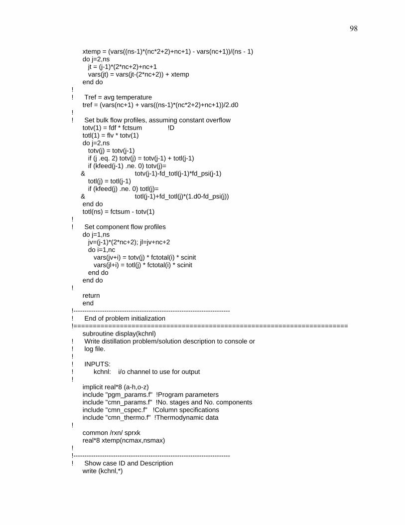
98

xtemp = (vars((ns-1)*(nc*2+2)+nc+1) - vars(nc+1))/(ns - 1) do j=2,ns jt = (j-1)*(2*nc+2)+nc+1 vars(jt) = vars(jt-(2*nc+2)) + xtemp end do ! ! Tref = avg temperature tref = (vars(nc+1) + vars((ns-1)*(nc*2+2)+nc+1))/2.d0 ! ! Set bulk flow profiles, assuming constant overflow totv(1) = fdf * fctsum !D totl(1) = flv * totv(1) do j=2,ns totv(j) = totv(j-1) if (j .eq. 2) totv(j) = totv(j-1) + totl(j-1) if (kfeed(j-1) .ne. 0) totv(j)= & totv(j-1)-fd_totl(j-1)*fd_psi(j-1) totl(j) = totl(j-1) if (kfeed(j) .ne. 0) totl(j)= & totl(j-1)+fd_totl(j)*(1.d0-fd_psi(j)) end do totl(ns) = fctsum - totv(1) ! ! Set component flow profiles do j=1,ns jv=(j-1)*(2*nc+2); jl=jv+nc+2 do i=1,nc vars(jv+i) = totv(j) * fctotal(i) * scinit vars(jl+i) = totl(j) * fctotal(i) * scinit end do end do ! return end !----------------------------------------------------------------------- ! End of problem initialization !======================================================================= subroutine display(kchnl) ! Write distillation problem/solution description to console or ! log file. ! ! INPUTS: ! kchnl: i/o channel to use for output ! implicit real*8 (a-h,o-z) include "pgm_params.f" !Program parameters include "cmn_params.f" !No. stages and No. components include "cmn_cspec.f" !Column specifications include "cmn_thermo.f" !Thermodynamic data ! common /rxn/ sprxk real*8 xtemp(ncmax,nsmax) ! !----------------------------------------------------------------------- ! Show case ID and Description write (kchnl,*)

99

write (kchnl,*)"Case ID: ", pdname_out write (kchnl,'(a)')c_desc ! !----------------------------------------------------------------------- ! Show thermodynamic model used ! write (kchnl,'(a$)')"Thermodynamic model: " ! if (kthermo .eq. 4) then ! write (kchnl,'(a)')"Van der Waals" ! else if (kthermo .eq. 3) then ! write (kchnl,'(a)')"Redlich-Kwong" ! else if (kthermo .eq. 2) then ! write (kchnl,'(a)')"Soave-Redlich-Kwong" ! else ! write (kchnl,'(a)')"Peng-Robinson" ! end if ! !----------------------------------------------------------------------- ! Show no. stages, no. components, and condenser type write (kchnl,'(2(a,i3),a$)')"Stages: ",ns," Components: ",nc, & " Condenser: " if (kcond .eq. 2) then write (kchnl,'(a)')"Partial" else write (kchnl,'(a)')"Total" end if ! !----------------------------------------------------------------------- ! Show component data (simplified system) write(kchnl,'(a)')"Component information:" write(kchnl,'(a)')" alpha Hv Hr"// &" CpL CpV Krx" write(kchnl,'(8x,6f10.2)')alpha,delhv,delhr,cpl,cpv,rxnke0 write(kchnl,'(a)')" nu Tb CpL"// &" CpV Hr" do i=1,nc write(kchnl,'(2x,a6,5f10.2)')cname(i),rxsto(i),tboil(i),cpa0(i), & cpa1(i),delhf(i) end do ! !----------------------------------------------------------------------- ! Show material balance and energy balance specifications do i=1,2 if (kspec(i) .eq. 3) then write(kchnl,*)"Overhead recovery (D/D+B): ",xspec(i) else if (kspec(i) .eq. 8) then write(kchnl,*)"Bottoms recovery (B/D+B): ",xspec(i) else if (kspec(i) .eq. 4) then write(kchnl,*)"Overhead recovery (di/di+bi): ",xspec(i), & " for ",cname(ispec(i)) else if (kspec(i) .eq. 7) then write(kchnl,*)"Bottoms recovery (b1/di+bi): ",xspec(i), & " for ",cname(ispec(i)) else if (kspec(i) .eq. 2) then write(kchnl,*)"Reflux ratio (L/D): ",xspec(i) else if (kspec(i) .eq. 5) then write(kchnl,*)"Condenser temperature: ",xspec(i)

100

else if (kspec(i) .eq. 1) then write(kchnl,*)"Condenser heat duty: ",xspec(i) else if (kspec(i) .eq. 9) then write(kchnl,*)"Boilup ratio (V/B): ",xspec(i) else if (kspec(i) .eq. 6) then write(kchnl,*)"Reboiler temperature: ",xspec(i) else if (kspec(i) .eq. 10) then write(kchnl,*)"Reboiler heat duty: ",xspec(i) end if end do ! !----------------------------------------------------------------------- ! Show reaction equilibrium constant if specified if (sprxk .ne. 0.d0) write(kchnl,*)"Specified Reaction K: ",sprxk ! !----------------------------------------------------------------------- ! Show column feeds write(kchnl,*)"Feeds:" do j=1,ns if (fd_temp(j) .ne. 0) then write(kchnl,1010)"Stg: ",j," Temp(K): ",fd_temp(j), & " Press(bar): ",fd_pres(j), & " Enthalpy(J): ",fd_enth(j) 1010 format(a,i3,a,f9.4,a,f9.4,a,f9.2) write(kchnl,*)" "," Liquid Vapor" do i=1,nc write(kchnl,'(a12,2f10.4)')cname(i),fd_liq(i,j), & fd_vap(i,j) end do end if end do ! !----------------------------------------------------------------------- ! Show Condenser and Reboiler duties. qc = (- fd_enth(1) - hstream(vars(2*nc+3),vars(3*nc+3),p(2),nc,1) & + (1.d0+sd_v(1))*hstream(vars(1),vars(nc+1),p(1),nc,kcond-1) & + (1.d0+sd_l(1))*hstream(vars(nc+3),vars(nc+1),p(1),nc,0)) & /1.d3 write(kchnl,*)"Condenser duty(kJ): ",qc jxr=(ns-1)*(2*nc+2); jxrm1=jxr-(2*nc+2) qr = (- fd_enth(ns) & - hstream(vars(jxrm1+nc+3),vars(jxrm1+nc+1),p(ns-1),nc,0) & + (1.d0+sd_v(1))*hstream(vars(jxr+1),vars(jxr+nc+1),p(ns),nc,1) & + (1.d0+sd_l(1)) & *hstream(vars(jxr+nc+3),vars(jxr+nc+1),p(ns),nc,0)) & /1.d3 write(kchnl,*)"Reboiler duty(kJ): ",qr ! !----------------------------------------------------------------------- ! Show pressure, temperature, heat duty, side draw, and ! efficiency profiles write(kchnl,*)"Column profiles:" write(kchnl,'(a)')"Stg Q(kJ) L s/d V s/d"// & " VLE eff Rxn eff Rx(mol) Rx(kJ)" do j=1,ns do i=1,nc

101

xtemp(i,j)=-vars((j-1)*(2*nc+2)+i)+fd_liq(i,j)+fd_vap(i,j) if (j .ne. 1)xtemp(i,j)=xtemp(i,j)+ & vars((j-2)*(2*nc+2)+nc+2+i) if (j .ne. ns)xtemp(i,j)=xtemp(i,j)+ & vars(j*(2*nc+2)+i) end do end do do j=1,ns rxx = rxex(xtemp(1,j),vars((j-1)*(2*nc+2)+nc+1),p(j),nc,0,0)* & rxeff(j) write (kchnl,1000)j,q(j),sd_l(j),sd_v(j),stg_mve(j),rxeff(j), & rxx,rxx*delhr/1.d3 end do 1000 format(i3,2x,7f11.4) ! !----------------------------------------------------------------------- ! Show Pressure, Temperature, Heat duty, and Bulk flow profiles. write(kchnl,'(a)')"Stg P(bar) T(K)"// & " L(mol) V(mol) H err L(kJ) V(kJ)" do j=1,ns jstg = (j-1)*(2*nc+2) totv(j) = 0.d0 totl(j) = 0.d0 do i=1,nc totv(j) = totv(j) + vars(jstg+i) totl(j) = totl(j) + vars(jstg+nc+2+i) vlk(i,j) = vler(vars(jstg+nc+3),vars(jstg+1), & vars(jstg+nc+1),p(j),nc,i) end do hvap(j) = hstream(vars(jstg+1),vars(jstg+nc+1),p(j),nc,1)/ & 1000.d0 if (j .eq. 1 .and. kcond .eq. 1)hvap(j) = hstream(vars(jstg+1), & vars(jstg+nc+1),p(j),nc,0)/1000.d0 hliq(j) = hstream(vars(jstg+nc+2+1),vars(jstg+nc+1),p(j),nc,0)/ & 1000.d0 rxk(j) = rxer(vars(jstg+nc+3),vars(jstg+nc+1),p(j),nc,0,0) end do do j=1,ns jstg = (j-1)*(2*nc+2) herr = fd_enth(j)+q(j)-hliq(j)-hvap(j) if (j .eq. 1 .and. q(j) .eq. 0.d0) herr = herr + qc if (j .eq. ns .and. q(j) .eq. 0.d0) herr = herr + qr if (j .ne. 1) herr = herr + hliq(j-1) if (j .ne. ns) herr = herr + hvap(j+1) write (kchnl,1000)j,p(j),vars(jstg+nc+1),totl(j),totv(j), & herr,hliq(j),hvap(j) write (kchnl,'(60x,2f11.4)')hliq(j)/totl(j),hvap(j)/totv(j) end do !----------------------------------------------------------------------- ! Show Vapor flow profiles write(kchnl,*)"Vapor flows/compositions:" do ii=1,nc,5 ij=ii+4 if (ij .ge. nc) ij=nc write(kchnl,'(9x,5a12)')(cname(i),i=ii,ij) do j=1,ns

102

jj=(j-1)*(2*nc+2) write(kchnl,'(i3,2x,5f12.4)')j,(vars(jj+i),i=ii,ij) write(kchnl,'(5x,5f12.6)')(vars(jj+i)/totv(j),i=ii,ij) end do end do ! !----------------------------------------------------------------------- ! Show Liquid flow profiles write(kchnl,*)"Liquid flows/compositions:" do ii=1,nc,5 ij=ii+4 if (ij .ge. nc) ij=nc write(kchnl,'(9x,5a12)')(cname(i),i=ii,ij) do j=1,ns jj=(j-1)*(2*nc+2)+nc+2 write(kchnl,'(i3,2x,5f12.4)')j,(vars(jj+i),i=ii,ij) write(kchnl,'(5x,5f12.6)')(vars(jj+i)/totl(j),i=ii,ij) end do end do ! !----------------------------------------------------------------------- ! Show component creation/consumption write(kchnl,*)"Component creation & consumption:" do j=1,ns do i=1,nc xtemp(i,j)=vars((j-1)*(2*nc+2)+i)+vars((j-1)*(2*nc+2)+nc+2+i) xtemp(i,j)=xtemp(i,j)-fd_liq(i,j)-fd_vap(i,j) if (j .ne. 1)xtemp(i,j)=xtemp(i,j)- & vars((j-2)*(2*nc+2)+nc+2+i) if (j .ne. ns)xtemp(i,j)=xtemp(i,j)- & vars(j*(2*nc+2)+i) end do end do do ii=1,nc,5 ij=ii+4 if (ij .ge. nc) ij=nc write(kchnl,'(9x,5a12)')(cname(i),i=ii,ij) do j=1,ns write(kchnl,'(i3,2x,5f12.4)')j,(xtemp(i,j),i=ii,ij) end do end do ! !----------------------------------------------------------------------- ! Show VLE equilibrium ratios write(kchnl,*)"Vapor/Liquid equilibrium ratios:" do ii=1,nc,5 ij=ii+4 if (ij .ge. nc) ij=nc write(kchnl,'(9x,5a12)')(cname(i),i=ii,ij) do j=1,ns jv=(j-1)*(2*nc+2) jl=jv+nc+2 write(kchnl,'(i3,2x,5e12.4)')j,(vlk(i,j),i=ii,ij) write(kchnl,'(5x,5e12.4)')(((vars(jv+i)*totl(j))/ & (vars(jl+i)*totv(j))),i=ii,ij) end do

103

end do ! !----------------------------------------------------------------------- ! Show Reaction equilibrium ratios write(kchnl,*)"Reaction equilibrium ratios:" write(kchnl,'(6x,a,2x,a)')"From thermo","From flows" do j=1,ns rktemp = 1.d0 do i=1,nc if (rxsto(i) .ne. 0.d0) rktemp=rktemp* & ((vars((j-1)*(2*nc+2)+nc+2+i)/totl(j))**rxsto(i)) end do write(kchnl,'(i3,2x,2e12.4)')j,rxk(j),rktemp end do ! !----------------------------------------------------------------------- ! Show Stream bubble and dew points write (kchnl,*)"Stream bubble/dew points:" write (kchnl,*)"Stg L bubble V dew" do j=1,ns jstg=(j-1)*(2*nc+2) dbub=bubpt(vars(jstg+nc+3),p(j)) ddew=dewpt(vars(jstg+1),p(j)) write(kchnl,'(i3,2x,2f10.4)')j,dbub,ddew end do return end ! !======================================================================= subroutine display2 ! Write solution description to console for excel ! implicit real*8 (a-h,o-z) include "pgm_params.f" !Program parameters include "cmn_params.f" !No. stages and No. components include "cmn_cspec.f" !Column specifications include "cmn_thermo.f" !Thermodynamic data ! real*8 xtemp(ncmax,nsmax) ! !----------------------------------------------------------------------- ! Show case ID write (*,*) write (*,*)"Case ID,", pdname_out ! !----------------------------------------------------------------------- ! Show Temperature and Bulk flow profiles. write(*,*)"j,T,L,V,L/V" do j=1,ns jstg = (j-1)*(2*nc+2) totv(j) = 0.d0 totl(j) = 0.d0 do i=1,nc totv(j) = totv(j) + vars(jstg+i) totl(j) = totl(j) + vars(jstg+nc+2+i)

104

end do end do do j=1,ns jstg = (j-1)*(2*nc+2) write (*,'(i3,4(",",f12.6))')j,vars(jstg+nc+1),totl(j), & totv(j),totl(j)/totv(j) end do !----------------------------------------------------------------------- ! Show Vapor composition profiles write(*,*)"y's" do j=1,ns jstg = (j-1)*(2*nc+2) write(*,'(i3,10(",",f12.6))')j,(vars(jstg+i)/totv(j),i=1,nc) end do ! !----------------------------------------------------------------------- ! Show Liquid composition profiles write(*,*)"x's" do j=1,ns jstg = (j-1)*(2*nc+2)+nc+2 write(*,'(i3,10(",",f12.6))')j,(vars(jstg+i)/totl(j),i=1,nc) end do ! !----------------------------------------------------------------------- ! Show component per stage conversion write(*,*)"Per stage conversion" do j=1,ns jstg = (j-1)*(2*nc+2) jm1 = jstg - (2*nc+2)+nc+2 jp1 = jstg + (2*nc+2) do i=1,nc xtemp(i,j)=fd_ctot(i,j) if (j .ne. 1)xtemp(i,j) =xtemp(i,j)+vars(jm1+i) if (j .ne. ns)xtemp(i,j)=xtemp(i,j)+vars(jp1+i) xtemp(i,j)=1.d0-(vars(jstg+i)+vars(jstg+nc+2+i))/xtemp(i,j) end do write(*,'(i3,10(",",f12.6))')j,(xtemp(i,j),i=1,nc) end do jm1 = 0 jp1 = (ns-1)*(2*nc+2) ! Show component overall conversion write(*,*)"Overall conversion" do i=1,nc xtemp(i,1)=0.d0 end do do j=1,ns do i=1,nc xtemp(i,1)=xtemp(i,1)+fd_ctot(i,j) end do end do do i=1,nc xtemp(i,2)=0.d0 if (xtemp(i,1) .ne. 0.d0) xtemp(i,2)=1.d0- & (vars(jm1+i)+vars(jp1+nc+2+i))/xtemp(i,1) end do write(*,'(i3,10(",",f12.6))')j,(xtemp(i,2),i=1,nc)

105

! !----------------------------------------------------------------------- ! Show Condenser and Reboiler duties. qc = (- fd_enth(1) - hstream(vars(2*nc+3),vars(3*nc+3),p(2),nc,1) & + (1.d0+sd_v(1))*hstream(vars(1),vars(nc+1),p(1),nc,kcond-1) & + (1.d0+sd_l(1))*hstream(vars(nc+3),vars(nc+1),p(1),nc,0)) & /1.d3 write(*,*)"Condenser duty(kJ),",qc jxr=(ns-1)*(2*nc+2); jxrm1=jxr-(2*nc+2) qr = (- fd_enth(ns) & - hstream(vars(jxrm1+nc+3),vars(jxrm1+nc+1),p(ns-1),nc,0) & + (1.d0+sd_v(1))*hstream(vars(jxr+1),vars(jxr+nc+1),p(ns),nc,1) & + (1.d0+sd_l(1)) & *hstream(vars(jxr+nc+3),vars(jxr+nc+1),p(ns),nc,0)) & /1.d3 write(*,*)"Reboiler duty(kJ),",qr ! !----------------------------------------------------------------------- return end ! !======================================================================= subroutine fdjac(x,fvec,df,n,NP) ! USES funcv implicit real*8 (a-h,o-z) PARAMETER (EPS=1.d-5) dimension df(np,np),fvec(np),x(np),f(np) ! Computes forward-difference approximation to Jacobian. On input, ! x(1:n) is the point at which the Jacobian is to be evaluated, ! fvec(1:n) is the vector of function values at the point, and np ! is the physical dimension of the Jacobian array df(1:n,1:n) which ! is output. subroutine funcv(n,x,f) is a fixed-name, user-supplied ! routine that returns the vector of functions at x. ! Parameters: EPS is the approximate square root of the machine ! precision. do j=1,n temp=x(j) h=EPS*abs(temp) if(h .eq. 0.d0)h=EPS x(j)=temp+h !Trick to reduce finite precision error. h=x(j)-temp call funcv(x, f, n, ierr) x(j)=temp do i=1,n !Forward difference formula. df(i,j)=(f(i)-fvec(i))/h end do end do return end ! !======================================================================= subroutine funcv(x,f,n,ierr) ! Calculate discrepancy function values f, for the column ! variables held in vector x. ! INPUTS:

106

! x : vector of column variables, as follows for each ! stage - nc vapor flows, 1 stage temperature, 1 stage ! reaction extent, and nc liquid flows. ! n : number of equations to evaluate - not used in this ! implementation. ! OUTPUTS: ! f : vector of calculated discrepancy function values - ! for each stage 1 energy balance, 1 reaction ! equilibrium function, nc material balances, ! and nc equilibrium relationships. ! ierr: error flag ( >0 if error) ! implicit real*8 (a-h,o-z) include "pgm_params.f" include "cmn_params.f" include "cmn_cspec.f" include "cmn_thermo.f" ! real*8 x(*),f(*) real*8 xt(ncmax) !vector of stage l-primes ! jn=2*nc+2 !no. equations per stage jfe1=1 !E function for condenser jfen=(ns-1)*jn+1 !E function for reboiler ! do j=1,ns !proceed stagewise, 1 to n jxv = (j-1)*jn !pointer to vapor flows jxt = jxv+nc+1 !Pointer to stage temp. jxx = jxt+1 !Pointer to stage rxn extent jxl = jxx !pointer to liquid flows jfe = (j-1)*jn+1 !pointer to energy bal function jfr = jfe+1 !pointer to rxn eq function jfm = jfr !pointer to matl bal functions jfq = jfm+nc !pointer to v/l equil functions ! ! calculate total stage flows tljm1 = 0.d0; tlj = 0.d0; tvj = 0.d0; tvjp1 = 0.d0 xmaxl = 0.d0; imaxl = 0 xtsum = 0.d0; eps = 0.d0 do i=1,nc tlj = tlj + x(jxl+i) tvj = tvj + x(jxv+i) xt(i) = fd_liq(i,j) + fd_vap(i,j) - (1.d0+sd_v(j))*x(jxv+i) if (j .ne. 1) then tljm1 = tljm1 + x(jxl-jn+i) xt(i) = xt(i) + x(jxl-jn+i) end if if (j .ne. ns) then tvjp1 = tvjp1 + x(jxv+jn+i) xt(i) = xt(i) + x(jxv+jn+i) end if if (x(jxl+i) .ge. xmaxl)then xmaxl = x(jxl+i) imaxl = i end if xtsum = xtsum + xt(i); eps = eps + rxsto(i)

107

end do ! do i=1,nc ! Material Balance Functions f(jfm+i)= -fd_liq(i,j)-fd_vap(i,j)-x(jxx)*rxsto(i)+ & (1.d0+sd_v(j))*x(jxv+i) + (1.d0+sd_l(j))*x(jxl+i) if (j .ne. 1) f(jfm+i) = f(jfm+i)-x(jxl-jn+i) if (j .ne. ns) f(jfm+i) = f(jfm+i)-x(jxv+jn+i) ! ! Vapor / Liquid Equilibrium functions if (j .eq. 1 .and. kcond .eq. 1)then vk = 1.d0 !total condenser else vk = vler(x(jxl+1),x(jxv+1),x(jxt),p(j),nc,i) !VLE K end if f(jfq+i) = stg_mve(j)*vk*x(jxl+i)/tlj - & x(jxv+i)/tvj if (j .ne. ns) f(jfq+i) = f(jfq+i) + & (1.d0-stg_mve(j))*x(jxv+jn+i)/tvjp1 ! f(jfq+i) = f(jfq+i) * 1.d2 !scale Q functions to M's end do ! Bubble point fn for total condenser if (j .eq. 1 .and. kcond .eq. 1)then f(jfq+imaxl) = 1.d0 do i=1,nc f(jfq+imaxl)=f(jfq+imaxl)- & vler(x(jxl+1),x(jxv+1),x(jxt),p(j),nc,i)* & x(jxl+i)/tlj end do ! f(jfq+imaxl) = f(jfq+imaxl) * 1.d2 !scale Q functions to M's end if ! ! Energy balance function f(jfe) = -q(j)-fd_enth(j) & +(1.d0+sd_l(j))*hstream(x(jxl+1),x(jxt),p(j),nc,0) if (j .eq. 1 .and. kcond .eq. 1)then !total condenser f(jfe) = f(jfe) + & (1.d0+sd_v(j))*hstream(x(jxv+1),x(jxt),p(j),nc,0) else f(jfe) = f(jfe) + & (1.d0+sd_v(j))*hstream(x(jxv+1),x(jxt),p(j),nc,1) end if if (j .ne. 1) f(jfe) = f(jfe) - & hstream(x(jxl-jn+1),x(jxt-jn),p(j-1),nc,0) if (j .ne. ns) f(jfe) = f(jfe) - & hstream(x(jxv+jn+1),x(jxt+jn),p(j+1),nc,1) ! f(jfe) = f(jfe)/1.d4 !Scale H functions to M's ! ! Reaction equilibrium function rxk(j) = rxer(xt,x(jxt),p(j),nc,i,0) if ((kinetic .and. holdupl(j) .eq. 0.d0) .or. (.not. kinetic & .and. rxeff(j) .eq. 0.d0))then f(jfr) = x(jxx) - 0.d0 !no reaction else if (kinetic) then !kinetic reaction model rxneff = 1.d0; rxntot = xtsum+rxneff*eps*x(jxx)

108

f2 = holdupl(j)*rxkf(xt,x(jxt),p(j),nc,i,0)/rxntot f1 = rxk(j)*f2; f3 = rxk(j)*x(jxx)/rxntot else !equilibrium reaction model rxneff = 1.d0/rxeff(j); rxntot = xtsum+rxneff*eps*x(jxx) f1 = rxk(j); f2 = 1.d0; f3 = 0.d0 end if do i=1,nc if (rxsto(i) .lt. 0.d0) then f1 = f1 * ((xt(i)+(rxneff*rxsto(i)*x(jxx)))/ & rxntot)**(-rxsto(i)) else if (rxsto(i) .gt. 0.d0) then f2 = f2 * ((xt(i)+(rxneff*rxsto(i)*x(jxx)))/ & rxntot)**rxsto(i) end if end do f(jfr) = f1 - f2 - f3 ! f(jfr) = f(jfr) * 1.d2 !Scale to M functions end if end do ! ! Substitute functions due to specifications ! set specification 1 if (kspec(1) .eq. 2) then !L/D spec dst = 0.d0; btm = 0.d0 do i=1,nc dst = dst + x(i) btm = btm + x(nc+2+i) end do f(jfe1) = btm/dst - xspec(1) ! f(jfe1) = f(jfe1)*1.d2 !scale to M functions else if (kspec(1) .eq. 3)then !D/F spec dst = 0.d0; btm = 0.d0 do i=1,nc dst = dst + x(i) ! btm = btm + x((ns-1)*jn+nc+2+i) end do do i=1,ns btm = btm + fd_totl(i) end do ! f(jfe1) = dst/(btm+dst) - xspec(1) f(jfe1) = dst/btm - xspec(1) ! f(jfe1) = f(jfe1)*1.d2 !scale to M functions else if (kspec(1) .eq. 4)then !Di/Fi spec dst = x(ispec(1)) btm = x((ns-1)*jn+nc+2+ispec(1)) f(jfe1) = dst/(dst+btm) - xspec(1) ! f(jfe1) = f(jfe1)*1.d2 !scale to M functions else if (kspec(1) .eq. 5)then !Tc spec f(jfe1) = x(nc+1) - xspec(1) ! f(jfe1) = f(jfe1)*1.d2 !scale to M functions else if (kspec(1) .eq. 11)then !L1 spec dst = 0.d0; btm = 0.d0 do i=1,nc dst = dst + x(nc+2+i) btm = btm + x((ns-1)*jn+i) end do

109

f(jfe1) = dst - xspec(1) else if (kspec(1) .eq. 12)then !Vn spec dst = 0.d0; btm = 0.d0 do i=1,nc dst = dst + x(nc+2+i) btm = btm + x((ns-1)*jn+i) end do f(jfe1) = btm - xspec(1) else if (kspec(1) .eq. 6)then !Tr spec f(jfe1) = x((ns-1)*jn+nc+1) - xspec(1) ! f(jfe1) = f(jfe1)*1.d2 !scale to M functions else if (kspec(1) .eq. 7)then !Bi/Fi spec dst = x(ispec(1)) btm = x((ns-1)*jn+nc+2+ispec(1)) f(jfe1) = btm/(dst+btm) - xspec(1) ! f(jfe1) = f(jfe1)*1.d2 !scale to M functions else if (kspec(1) .eq. 8)then !B/F spec dst = 0.d0; btm = 0.d0 do i=1,nc ! dst = dst + x(i) btm = btm + x((ns-1)*jn+nc+2+i) end do do i=1,ns dst = dst + fd_totl(i) end do ! f(jfe1) = btm/(btm+dst) - xspec(1) f(jfe1) = btm/dst - xspec(1) ! f(jfe1) = f(jfe1)*1.d2 !scale to M functions else if (kspec(1) .eq. 9)then !V/B spec dst = 0.d0; btm = 0.d0 do i=1,nc dst = dst + x((ns-1)*jn+i) btm = btm + x((ns-1)*jn+nc+2+i) end do f(jfe1) = dst/btm - xspec(1) ! f(jfe1) = f(jfe1)*1.d2 !scale to M functions end if ! ! set specification 2 if (kspec(2) .eq. 2) then !L/D spec dst = 0.d0; btm = 0.d0 do i=1,nc dst = dst + x(i) btm = btm + x(nc+2+i) end do f(jfen) = btm/dst - xspec(2) ! f(jfen) = f(jfen)*1.d2 !scale to M functions else if (kspec(2) .eq. 3)then !D/F spec dst = 0.d0; btm = 0.d0 do i=1,nc dst = dst + x(i) ! btm = btm + x((ns-1)*jn+nc+2+i) end do do i=1,ns btm = btm + fd_totl(i) end do

110

! f(jfen) = dst/(btm+dst) - xspec(2) f(jfen) = dst/btm - xspec(2) ! f(jfen) = f(jfen)*1.d2 !scale to M functions else if (kspec(2) .eq. 4)then !Di/Fi spec dst = x(ispec(2)) btm = x((ns-1)*jn+nc+2+ispec(2)) f(jfen) = dst/(dst+btm) - xspec(2) ! f(jfen) = f(jfen)*1.d2 !scale to M functions else if (kspec(2) .eq. 5)then !Tc spec f(jfen) = x(nc+1) - xspec(2) ! f(jfen) = f(jfen)*1.d2 !scale to M functions else if (kspec(2) .eq. 6)then !Tr spec f(jfen) = x((ns-1)*jn+nc+1) - xspec(2) ! f(jfen) = f(jfen)*1.d2 !scale to M functions else if (kspec(2) .eq. 7)then !Bi/Fi spec dst = x(ispec(2)) btm = x((ns-1)*jn+nc+2+ispec(2)) f(jfen) = btm/(dst+btm) - xspec(2) ! f(jfen) = f(jfen)*1.d2 !scale to M functions else if (kspec(2) .eq. 8)then !B/F spec dst = 0.d0; btm = 0.d0 do i=1,nc ! dst = dst + x(i) btm = btm + x((ns-1)*jn+nc+2+i) end do do i=1,ns dst = dst + fd_totl(i) end do ! f(jfen) = btm/(btm+dst) - xspec(2) f(jfen) = btm/dst - xspec(2) ! f(jfen) = f(jfen)*1.d2 !scale to M functions else if (kspec(2) .eq. 9)then !V/B spec dst = 0.d0; btm = 0.d0 do i=1,nc dst = dst + x((ns-1)*jn+i) btm = btm + x((ns-1)*jn+nc+2+i) end do f(jfen) = dst/btm - xspec(2) ! f(jfen) = f(jfen)*1.d2 !scale to M functions else if (kspec(2) .eq. 11)then !L1 spec dst = 0.d0; btm = 0.d0 do i=1,nc dst = dst + x(nc+2+i) btm = btm + x((ns-1)*jn+i) end do f(jfen) = dst - xspec(2) else if (kspec(2) .eq. 12)then !Vn spec dst = 0.d0; btm = 0.d0 do i=1,nc dst = dst + x(nc+2+i) btm = btm + x((ns-1)*jn+i) end do f(jfen) = btm - xspec(2) end if ! ierr = 0

111

! return end ! !======================================================================= ! Include subroutine packages ! include "altthermo.f" include "newton.f" include "homotopy.f" ALTTHERMO.F subroutine flash(kf, zf, tf, pf, pstg, xf, yf, hf,ftotal,psi) ! Computes the flash of stream zf to form streams xf and yf ! Inputs: ! kf : flash type ! zf : vector containing feed compositions or flows ! tf : flash temperature ! pf : flash pressure ! pstg: ? ! Outputs: ! xf : vector of output liquid compositions or flows ! yf : vector of output vapor compositions or flows ! hf : ! ftotal: ! psi : Fraction of feed leaving as vapor ! ! Specification statements: implicit real*8 (a-h,o-z) ! Set parameter values include "pgm_params.f" parameter (itmax = 25, xacc = 1.d-6) ! Define data storage include "cmn_params.f" real*8 zf(ncmax), xf(ncmax), yf(ncmax), z(ncmax), x(ncmax), & y(ncmax), vlek(ncmax), ftotal, psi, tbp, tdp fpsi(psi, i) = z(i)*(1.d0-vlek(i))/(1.d0+psi*(vlek(i)-1.d0)) ftmp(t,i) = z(i)*(1.d0-vler(z,z,t,pstg,nc,i))/ & (1.d0+psi*(vler(z,z,t,pstg,nc,i)-1.d0)) ! ! Normalize feed vector and calculate dew and bubble points ftotal = 0.d0 do i=1,nc ftotal = ftotal + zf(i) end do do i=1,nc z(i) = zf(i)/ftotal; x(i) = 0.d0; y(i) = 0.d0 end do tbp = bubpt(z, pstg) tdp = dewpt(z, pstg) if (kf .eq. 1) then ! Bubble point liquid feed tf = tbp hf=hstream(zf,tf,pf,nc,0)

112

do i=1,nc xf(i) = zf(i); yf(i) = 0.d0 end do psi = 0.d0 else if (kf .eq. 2) then ! Dew point vapor feed tf = tdp hf=hstream(zf,tf,pf,nc,1) do i=1,nc yf(i) = zf(i); xf(i) = 0.d0 end do psi = 1.d0 else if (kf .eq. 3) then ! Spec temp flash if (tf .ge. tdp) then !T above dew point do i=1,nc yf(i) = zf(i); xf(i) = 0.d0 end do psi = 1.d0 hf=hstream(zf,tf,pf,nc,1) else if (tf .le. tbp) then !T below bubble point do i=1,nc xf(i) = zf(i); yf(i) = 0.d0 end do psi = 0.d0 hf=hstream(zf,tf,pf,nc,0) else !T between dew & bubble pts psi1 = 0.d0 psi2 = 1.d0 f1 = 0.d0 f2 = 0.d0 psi = -1 do i=1,nc vlek(i) = vler(z,z,tf,pstg,nc,i) f1 = f1 + fpsi(psi1, i) f2 = f2 + fpsi(psi2, i) end do do n=1,itmax psi3 = 0.5d0*(psi1+psi2) f3 = 0.d0 do i=1,nc f3 = f3 + fpsi(psi3, i) end do psi4 = psi3 + (psi3 - psi1)*(sign(1.d0, f1-f2)*f3 & /sqrt(f3**2 - f1*f2)) if (abs(psi4-psi) .le. xacc) then exit end if psi = psi4 f4 = 0.d0 do i=1,nc f4 = f4 + fpsi(psi4, i) end do if (f4 .eq. 0.d0) then end if if (sign(f3, f4) .ne. f3) then psi1 = psi3; f1 = f3; psi2 = psi4; f2 = f4 else if (sign(f1, f4) .ne. f1) then

113

psi2 = psi4; f2 = f4 else if (sign(f2, f4) .ne. f2) then psi1 = psi4; f1 = f4 end if end do do i=1,nc x(i) = z(i) / (1.d0+psi*(vlek(i)-1.d0)) y(i) = x(i)*vlek(i) xf(i) = ftotal * (1.d0-psi) * x(i) yf(i) = ftotal * psi *y(i) end do hf=psi*hstream(zf,tf,pf,nc,1) + & (1.d0-psi)*hstream(zf,tf,pf,nc,0) end if else if (kf .eq. 4) then !Spec V/F flash if (psi .le. 0.d0) then !All liquid do i=1,nc xf(i) = zf(i); yf(i) = 0.d0 end do tf = tbp hf = hstream(zf,tf,pf,nc,0) else if (psi .ge. 1.d0) then !All vapor do i=1,nc yf(i) = zf(i); xf(i) = 0.d0 end do tf = tdp hf = hstream(zf,tf,pf,nc,1) else t1 = tbp; f1 = 0.d0 t2 = tdp; f2 = 0.d0 tf = -1.d0 do i=1,nc f1 = f1+ftmp(t1,i) f2 = f2+ftmp(t2,i) end do do n=1,itmax t3 = 0.5d0*(t1+t2); f3 = 0.d0 do i=1,nc f3 = f3+ftmp(t3,i) end do t4 = t3 + (t3-t1)*(sign(1.d0,f1-f2)*f3 & /sqrt(f3**2 - f1*f2)) if (abs(t4-tf) .le. xacc) then exit end if tf = t4; f4 = 0.d0 do i=1,nc f4 = f4+ftmp(t4,i) end do if (f4 .eq. 0.d0) then end if if (sign(f3,f4) .ne. f3)then t1 = t3; f1 = f3; t2 = t4; f2 = f4 else if (sign(f1,f4) .ne. f1) then t2 = t4; f2 = f4 else if (sign(f2,f4) .ne. f2) then

114

t1 = t4; f1 = f4 end if end do do i=1,nc vlek(i) = vler(z,z,tf,pstg,nc,i) x(i) = z(i) / (1.d0+psi*(vlek(i)-1.d0)) y(i) = x(i) * vlek(i) xf(i) = ftotal * (1.d0-psi) * x(i) yf(i) = ftotal * psi * y(i) end do hf = psi*hstream(zf,tf,pf,nc,1) + & (1.d0-psi)*hstream(zf,tf,pf,nc,0) end if end if return end !======================================================================= real*8 function bubpt(x,p) ! Computes bubblepoint temperature of stream x at pressure p ! ! Specification statements: implicit real*8 (a-h,o-z) ! Set parameter values include "pgm_params.f" parameter (itmax = 50, xacc = 1.d-6, factor = 1.6d0) ! Define data storage include "cmn_params.f" include "cmn_thermo.f" ! real*8 x(ncmax),xnorm(ncmax) ! ! Normalize x xnormsum=0.d0 do i=1,nc xnormsum=xnormsum+x(i) end do do i=1,nc xnorm(i)=x(i)/xnormsum end do ! Use component boil points to start t1 = tboil(1) t2 = tboil(nc) f1 = 1.d0 f2 = 1.d0 bubpt = -1.d0 do i=1,nc f1 = f1 - xnorm(i) * vler(xnorm,xnorm,t1,p,nc,i) f2 = f2 - xnorm(i) * vler(xnorm,xnorm,t2,p,nc,i) end do do n=1,itmax ! make sure point is bracketed if (f1*f2 .lt. 0.d0) exit if (abs(f1) .lt. abs(f2)) then t1 = t1+factor*(t1-t2) f1 = 1.d0 do i=1,nc

115

f1 = f1 - xnorm(i) * vler(xnorm,xnorm,t1,p,nc,i) end do else t2 = t2+factor*(t2-t1) f2 = 1.d0 do i=1,nc f2 = f2 - xnorm(i) * vler(xnorm,xnorm,t2,p,nc,i) end do end if end do if (f1*f2 .ge. 0.d0) write(*,*)"BUBPT: Failed to find range." do n=1,itmax ! search for best value t3 = 0.5d0*(t1+t2) f3 = 1.d0 do i=1,nc f3 = f3 - xnorm(i) * vler(x,x,t3,p,nc,i) end do t4 = t3 + (t3 - t1)*(sign(1.d0, f1-f2)*f3/sqrt(f3**2 - f1*f2)) if (abs(t4-bubpt) .le. xacc) return bubpt = t4 f4 = 1.d0 do i=1,nc f4 = f4 - xnorm(i) * vler(x,x,t4,p,nc,i) end do if (f4 .eq. 0.d0) return if (sign(f3, f4) .ne. f3) then t1 = t3; f1 = f3; t2 = t4; f2 = f4 else if (sign(f1, f4) .ne. f1) then t2 = t4; f2 = f4 else if (sign(f2, f4) .ne. f2) then t1 = t4; f1 = f4 end if if (abs(t2 - t1) .le. xacc) return end do write (*,*) "BUBPT: fails to converge in ",itmax," iterations" write(*,*)"BUBPT: Returned value is: ",bubpt return end !======================================================================= real*8 function dewpt(x,p) ! Computes dewpoint temperature of stream x at pressure p ! ! Specification statements: implicit real*8 (a-h,o-z) ! Set parameter values include "pgm_params.f" parameter (itmax = 50, xacc = 1.d-6, factor = 1.6d0) ! Define data storage include "cmn_params.f" include "cmn_thermo.f" ! real*8 x(ncmax),xnorm(ncmax) ! ! Normalize x xnormsum=0.d0 do i=1,nc

116

xnormsum=xnormsum+x(i) end do do i=1,nc xnorm(i)=x(i)/xnormsum end do ! Use component boil points to start t1 = tboil(1) t2 = tboil(nc) f1 = 1.d0 f2 = 1.d0 dewpt = -1.d0 do i=1,nc f1 = f1 - xnorm(i) / vler(xnorm,xnorm,t1,p,nc,i) f2 = f2 - xnorm(i) / vler(xnorm,xnorm,t2,p,nc,i) end do do n=1,itmax ! make sure point is bracketed if (f1*f2 .lt. 0.d0) exit if (abs(f1) .lt. abs(f2)) then t1 = t1+factor*(t1-t2) f1 = 1.d0 do i=1,nc f1 = f1 - xnorm(i) / vler(xnorm,xnorm,t1,p,nc,i) end do else t2 = t2+factor*(t2-t1) f2 = 1.d0 do i=1,nc f2 = f2 - xnorm(i) / vler(xnorm,xnorm,t2,p,nc,i) end do end if end do if (f1*f2 .ge. 0.d0) write(*,*)"DEWPT: Failed to find range." do n=1,itmax ! search for best value t3 = 0.5d0*(t1+t2) f3 = 1.d0 do i=1,nc f3 = f3 - xnorm(i) / vler(xnorm,xnorm,t3,p,nc,i) end do t4 = t3 + (t3 - t1)*(sign(1.d0, f1-f2)*f3/sqrt(f3**2 - f1*f2)) if (abs(t4-dewpt) .le. xacc) return dewpt = t4 f4 = 1.d0 do i=1,nc f4 = f4 - xnorm(i) / vler(xnorm,xnorm,t4,p,nc,i) end do if (f4 .eq. 0.d0) return if (sign(f3, f4) .ne. f3) then t1 = t3; f1 = f3; t2 = t4; f2 = f4 else if (sign(f1, f4) .ne. f1) then t2 = t4; f2 = f4 else if (sign(f2, f4) .ne. f2) then t1 = t4; f1 = f4 end if if (abs(t2 - t1) .le. xacc) return end do

117

write (*,*) "DEWPT: fails to converge in ",itmax," iterations" write(*,*)"DEWPT: Returned value is: ",dewpt return end !======================================================================= real*8 function rxex(x,t,pstg,nc,ic,kst) ! Compute the equilibrium extent of reaction at t and p ! Inputs: ! x : vector of stream compositions or flows ! t : temperature for the calculation, K ! p : pressure for the calculation, bar ! nc : number of components in x ! ic : component index (not used in this calc'n) ! kst: Stream state (0=>liquid; 1=>vapor) ! Outputs: ! rxex: Calculated extent of reaction ! implicit real*8 (a-h,o-z) include "pgm_params.f" !Storage allocation parameters include "cmn_thermo.f" !component thermodynamic data dimension x(*) parameter (gs = 0.381966011d0) !parm for golden section search ! rxek = rxer(x,t,pstg,nc,ic,kst) !Get the equilibrium constant xmax = 1.d20 xmin = -1.d20 xsum = 0.d0 eps = 0.d0 do i=1,nc !find max fwd and rev extents xsum = xsum + x(i) eps = eps + rxsto(i) if (rxsto(i) .ne. 0.d0) then xtemp = - x(i) / rxsto(i) if (rxsto(i) .lt. 0.d0 .and. xtemp .lt. xmax) xmax = xtemp if (rxsto(i) .gt. 0.d0 .and. xtemp .gt. xmin) xmin = xtemp end if end do ! Initialize for Brent method search to find the root a = xmin; b = xmax fa1 = 1.d0; fa2 = rxek fb1 = 1.d0; fb2 = rxek do i=1,nc !f(x) = product of factor, minus rxek if (rxsto(i) .gt. 0.d0) then fa1=fa1*((x(i)+rxsto(i)*a)/(xsum+eps*a))**rxsto(i) fb1=fb1*((x(i)+rxsto(i)*b)/(xsum+eps*b))**rxsto(i) else if (rxsto(i) .lt. 0.d0) then fa2=fa2*((x(i)+rxsto(i)*a)/(xsum+eps*a))**(-rxsto(i)) fb2=fb2*((x(i)+rxsto(i)*b)/(xsum+eps*b))**(-rxsto(i)) end if end do fa=fa1-fa2; fb=fb1-fb2 ! fa=fa-rxek; fb=fb-rxek c = b; fc = fb do k=1,100 !search loop if (fb*fc .ge. 0.d0) then ! Rename a,b,&c and adjust bounding interval d

118

c=a; fc=fa; d=b-a; e=d end if if (abs(fc) .lt. abs(fb)) then !swap a and c with b a=b; b=c; c=a fa=fb; fb=fc; fc=fa end if tol1 = 2.d0*1.d-8*abs(b) + 0.5d0*1.d-8 !check convergence xm = 0.5d0*(c-b) if (abs(xm) .le. tol1 .or. fb .eq. 0.d0) then !Converged rxex = b return end if if (abs(e) .gt. tol1 .and. abs(fa) .gt. abs(fb)) then ! Try inverse quadratic interpolation s = fb/fa if (a .eq. c) then p = 2.d0*xm*s q = 1.d0 - s else q = fa/fc r = fb/fc p = s*(2.d0*xm*q*(q-r)-(b-a)*(r-1.d0)) q = (q-1.d0)*(r-1.d0)*(s-1.d0) end if if (p .gt. 0.d0) q = -q !Check whether in bounds p = abs(p) if (2.d0*p .lt. min(3.d0*xm*q-abs(tol1*q), abs(e*q))) then e=d !Accept interpolation d=p/q else d=xm !Interpolation failed, use bisection e=d end if else d=xm !Bounds decreasing too slowly, use bisection e=d end if a=b !Move last guess to a fa=fb if (abs(d) .gt. tol1) then !Evaluate new trial root b=b+d else b=b+sign(tol1,xm) end if fb1=1.d0; fb2=rxek !Compute function value for new trial root do i=1,nc if (rxsto(i) .gt. 0.d0) then fb1 = fb1*((x(i)+rxsto(i)*b)/(xsum+eps*b))**rxsto(i) else if (rxsto(i) .lt. 0.d0) then fb2 = fb2*((x(i)+rxsto(i)*b)/(xsum+eps*b))**(-rxsto(i)) end if end do fb=fb1-fb2 end do rxex = b write (*,*)"Reaction extent = ",rxex," Excess Iterations"

119

return end !======================================================================= real*8 function vler(x,y,t,p,nc,ic) ! Computes the vapor-liquid equilibrium ratio for ! component ic in the mixture x at t and p ! Inputs: ! x : vector of liquid stream compositions or flows ! y : vector of vapor stream compositions or flows ! t : temperature for the calculation, K ! p : pressure for the calculation, bar ! nc : number of components in x ! ic : index of the component of interest ! Outputs: ! vler: Calculated value of the property ! implicit real*8 (a-h,o-z) include "pgm_params.f" !Storage allocation parameters include "cmn_thermo.f" !component thermodynamic data dimension x(*),y(*) ! vler = exp( vpa(ic) - vpb(ic)/t ) / p ! vler =exp(-((1.d0/t)-(1.d0/tboil(ic)))*delhv/rgas) return end !======================================================================= real*8 function hstream(x,t,p,nc,kst) ! Compute the enthalpy of stream x at t and p in state kst, ! relative to tref. Value returned is in units of kJ ! Inputs: ! x : vector of stream compositions or flows ! t : temperature for the calculation, K ! p : pressure for the calculation, bar ! nc : number of components in x ! kst: Stream state (0=>liquid; 1=>vapor) ! Outputs: ! hstream: Calculated enthalpy, kJ ! implicit real*8 (a-h,o-z) include "pgm_params.f" !Storage allocation parameters include "cmn_thermo.f" !component thermodynamic data dimension x(*) ! t0 = tref !Reference Temp hstream = 0.d0 xsum = 0.d0 do i=1,nc xsum = xsum+x(i) end do if (kst .eq. 0) then do i=1,nc !liquid enthalpy hstream = hstream + ((t-t0)*cpa0(i)+delhf(i))*x(i)/xsum ! hstream = hstream + ((t-t0)*cpa0(i))*x(i)/xsum end do else ! hstream = delhv/xsum

120

do i=1,nc !vapor enthalpy hstream = hstream + ((tboil(i)-t0)*cpa0(i) + (t-tboil(i)) & *cpa1(i) + delhf(i) + delhv)*x(i)/xsum ! hstream = hstream + ((tboil(i)-t0)*cpa0(i) + (t-tboil(i)) ! & *cpa1(i))*x(i)/xsum end do end if hstream = hstream * xsum !change molar to total !kJ return end !======================================================================= real*8 function rxer(x,t,p,nc,ic,kst) ! Compute the reaction equilibrium constant at t and p ! Inputs: ! x : vector of stream compositions or flows ! t : temperature for the calculation, K ! p : pressure for the calculation, bar ! nc : number of components in x ! ic : component index (not used in this calc'n) ! kst: Stream state (0=>liquid; 1=>vapor) ! Outputs: ! rxer: Calculated value of the equilibrium constant ! implicit real*8 (a-h,o-z) include "pgm_params.f" !Storage allocation parameters include "cmn_thermo.f" !component thermodynamic data dimension x(*) rxer = rxnke0*exp(((1.d0/rxntref)-(1.d0/t))*rxeeql/rgas) ! return end !======================================================================= real*8 function rxkf(x,t,p,nc,ic,kst) ! Compute the reaction forward rate constant at t and p ! Inputs: ! x : vector of stream compositions or flows ! t : temperature for the calculation, K ! p : pressure for the calculation, bar ! nc : number of components in x ! ic : component index (not used in this calc'n) ! kst: Stream state (0=>liquid; 1=>vapor) ! Outputs: ! rxkf: Calculated value of the rate constant ! implicit real*8 (a-h,o-z) include "pgm_params.f" !Storage allocation parameters include "cmn_thermo.f" !component thermodynamic data dimension x(*) rxkf = rxkf0*exp(((1.d0/rxntref)-(1.d0/t))*rxefwd/rgas) ! return end !======================================================================= real*8 function boiltemp(ic,p) ! Compute the boiling temperature for component ic at pressure p ! Inputs:

121

! ic : component index ! p : pressure for the calculation, bar ! Outputs: ! boiltemp: Calculated value of the boiling temperature ! implicit real*8 (a-h,o-z) include "pgm_params.f" !Storage allocation parameters include "cmn_thermo.f" !component thermodynamic data boiltemp = vpb(ic)/(vpa(ic) - log(p)) ! return end !======================================================================= STATE.F subroutine dumpstate !Subroutine to dump complete problem specification and state ! ! ! Include files include "cmn_params.f" !no. stages & no. components include "cmn_cspec.f" !Problem specifications include "cmn_thermo.f" !Thermodynamic properties include "cmn_hsparms.f" !Homotopy parameters ! !Open file for output open (20, file = filename(1:lnblnk(filename))//'.dat') ! !Write ns and nc write(20) ns,nc !Write homotopy solver parameters write(20) dir, dso, dsmin, dsmax, xmax, & ecorc, ecorb, edet, esol, ebif, etur, esta, easy, & idom, ihom, maxdet, minasy, maxasy !Write thermodynamic stuff write(20) (cname(i), cmolwt(i), tmelt(i), & tboil(i), tcrit(i), pcrit(i), vcrit(i), & zcrit(i), acfac(i), delhf(i), delgf(i), & tcpmin(i), tcpmax(i), cpa0(i),cpa1(i), & cpa2(i), cpa3(i), cpa4(i),vpa(i), vpb(i), & vpc(i), pvpmin(i), pvpmax(i), tvpmin(i), & tvpmax(i),rxsto(i),fwvl(i),i=1,nc) write(20) acvl, bcvl, zcvl, uvl, wvl, fuwvl, & rgas, alpha, tb1, delhv, delhr, cpl, cpv, tref, & rxnke0, rxeeql, rxkf0, rxefwd, rxntref, kthermo, & kinetic !Write problem specification write(20) kcond, psname_in, pdname_out, c_desc write(20) (xspec(i), kspec(i), ispec(i), jspec(i),i=1,2) write(20) (fd_temp(i), fd_pres(i), fd_enth(i), & fd_totl(i), fd_psi(i), p(i), q(i), & sd_l(i), sd_v(i), stg_mve(i), rxeff(i), & holdupl(i), totl(i), totv(i), hliq(i), & hvap(i), rxk(i), kfeed(i), i=1,ns) write(20) ((fd_liq(j,i), fd_vap(j,i), fd_ctot(j,i),

122

& vlk(j,i),j=1,nc),i=1,ns) write(20) (vars(i), vars0(i),i=0,ns*(2*nc+2)) ! close(20) return end NEWTON.F subroutine nsolver(x,n,tolx,tolf,ntrial,kstatus,its,errf,ipr1, & ipr2) ! ! Use Newton iteration to improve a root x. ! Given an initial guess x for a root in n dimensions, take ntrial ! Newton-Raphson steps to improve the root. Stop if the root ! converges in either summed absolute variable increments tolx ! or summed absolute function values tolf. ! ! Reference: W.H.Press, B.P.Flannery, S.A.Teukolsky, and ! W.T.Vetterling, Numerical Recipes: The Art of ! Scientific Computing, Cambridge University Press, ! New York, NY, 1989. ! ! uses: nlubksb, nludcmp, ... ! ! Input Variables ! x: vector containing initially guessed variable values ! n: dimension of vector x ! tolx: lower limit of absolute variable increments ! tolf: lower limit of absolute function values ! ntrial: number of iterations allowed ! ! Output Variables ! x: vector of improved variable values ! kstatus: 0 if converged, -1 if not ! its: number of iterations performed ! errf: L2 norm of residual vector at completion ! ! input / output variables: integer n, ntrial, np real*8 tolf, tolx, x(n) ! ! local variables integer i, j, k, indx(n),imax real*8 d, errf, errx, fjac(n,n),fjaclu(n,n), fvec(n), p(n),p0(n), & p1(n),chmax,w(n),v(n,n),sum,ratio,temp,fvecx(n),f,fplus,gs, & fminus,xtemp(n),nvecnrm,xa,fxa,xb,fxb,x1,fx1,x2,fx2,fin(30) real*8 rcmax,rcmin,smlnum,bignum,rowcnd,rscale(n),fmax,fmin real*8 xlim,xlim1 real*8 bigchg, smlchg, chg, avchg ! include "cmn_params.f" parameter (gs = 0.381966011d0) !parm for golden section search ! big & small numbers parameter (smlnum = 2.22507386d-308,bignum = 1.d0/smlnum) !-----------------------------------------------------------------------

123

kstatus = 0 !Status okay unless a problem happens do k=1,ntrial !Iteration loop starts here its=k call funcv(x,fvec,n,ierr) !Get the function vector errf = nvecnrm(fvec,n) !Compute norm of the residual if (errf .le. tolf) return do i=1,n p(i) = -fvec(i) end do call fdjac(x,fvec,fjac,n,n) !Get the jacobian of the function !----------------------------------------------------------------------- ! Scale the jacobian and the p vector to prevent overflows rcmax = smlnum rcmin = bignum do i=1,n !Scan rows for largest element rscale(i) = 0.d0 do j=1,n rscale(i) = max(rscale(i), abs(fjac(i,j))) end do rcmax = max(rcmax,rscale(i)) rcmin = min(rcmin,rscale(i)) if (rcmin .eq. 0.d0) then !Bail out if singular write (ipr1,*)"SOLVER: Singular Jacobian for function ",i kstatus = -1 return end if rscale(i) = 1.d0 / min(max(rscale(i),smlnum),bignum) end do rowcnd = max(rcmin,smlnum)/min(rcmax,bignum) do i=1,n !Scale the system p(i) = p(i) * rscale(i) do j=1,n fjac(i,j) = fjac(i,j) * rscale(i) end do end do !----------------------------------------------------------------------- call nludcmp(fjac, n, n, indx, d) call nlubksb(fjac, n, n, indx, p) !----------------------------------------------------------------------- ! Limit temperature changes xlim = 10.d0 xlim1 = 1.2d0 do j=1,ns jl=(j-1)*(2*nc+1) jv=(j-1)*(2*nc+1)+nc+1 jt=(j-1)*(2*nc+1)+nc+1 p(jt)=sign(xlim*(1.d0-exp(-xlim1*abs(p(jt)/xlim))),p(jt)) do i=1,nc !Limit flow changes to stay positive if (p(jl+i) .lt. -0.8d0*x(jl+i)) p(jl+i) = -0.8d0*x(jl+i) if (p(jv+i) .lt. -0.8d0*x(jv+i)) p(jv+i) = -0.8d0*x(jv+i) end do end do ! limit flow changes here, too ?? !----------------------------------------------------------------------- ! golden section search for optimum distance along the p vector xa = 0.15d0

124

do i=1,n xtemp(i) = x(i) + xa*p(i) end do call funcv(xtemp,fvecx,n,ierr) fxa = nvecnrm(fvecx,n) xb = 1.25d0 do i=1,n xtemp(i) = x(i) + xb*p(i) end do call funcv(xtemp,fvecx,n,ierr) fxb = nvecnrm(fvecx,n) nfi = 20 x1 = xa + (xb-xa)*gs do i=1,n xtemp(i) = x(i) + x1*p(i) end do call funcv(xtemp,fvecx,n,ierr) fx1 = nvecnrm(fvecx,n) x2 = xb - (xb-xa)*gs do i=1,n xtemp(i) = x(i) + x2*p(i) end do call funcv(xtemp,fvecx,n,ierr) fx2 = nvecnrm(fvecx,n) do kfi=1,nfi-1 !GS search loop if (fx1 .lt. fx2) then xb = x2; fxb = fx2 x2 = x1; fx2 = fx1 x1 = xa + (xb-xa)*gs do i=1,n xtemp(i) = x(i) + x1*p(i) end do call funcv(xtemp,fvecx,n,ierr) fx1 = nvecnrm(fvecx,n) ratio = x1 else xa = x1; fxa = fx1 x1 = x2; fx1 = fx2 x2 = xb - (xb-xa)*gs do i=1,n xtemp(i) = x(i) + x2*p(i) end do call funcv(xtemp,fvecx,n,ierr) fx2 = nvecnrm(fvecx,n) ratio = x2 end if end do do i=1,n !Adjust the p(i) to reflect damping p(i) = ratio * p(i) end do ! !----------------------------------------------------------------------- errx = 0.d0 do i=1,n errx = errx + abs(p(i)) x(i) = x(i) + p(i)

125

if (x(i) .le. 1.d-12) x(i) = 1.d-12 end do write (ipr1,*)"Iteration: ",k," Damping factor ",ratio, & " Error: ",errx if (errx .le. tolx) return end do kstatus=-1 return end ! !======================================================================= subroutine nludcmp(a,n,np,indx,d) integer n,np,indx(n),nmax real*8 d,a(np,np),tiny parameter (nmax=500,tiny=1.d-20) !largest expected n, and a small number. ! given a matrix a(1:n,1:n), with physical dimension np by np, ! this routine replaces it by the lu decomposition of a rowwise ! permutation of itself. a and n are input. a is output, arranged ! as in equation (2.3.14) above; indx(1:n) is an output vector ! that records the row permutation effected by the partial ! pivoting; d is output as ±1 depending on whether the number of ! row interchanges was even or odd, respectively. this routine is ! used in combination with nlubksb to solve linear equations or ! invert a matrix. integer i,imax,j,k real*8 aamax,dum,sum,vv(nmax) !vv stores the implicit scaling of each row. d=1.d0 !no row interchanges yet. do i=1,n !loop over rows to get the implicit scaling information. aamax=0.d0 do j=1,n if (abs(a(i,j)).gt.aamax) aamax=abs(a(i,j)) end do if (aamax .eq. 0.d0) then ! pause "singular matrix in nludcmp" !no nonzero largest element. d=0.d0 return end if vv(i)=1.d0/aamax !save the scaling. end do do j=1,n !this is the loop over columns of crout’s method. do i=1,j-1 !this is equation (2.3.12) except for i = j. sum=a(i,j) do k=1,i-1 sum=sum-a(i,k)*a(k,j) end do a(i,j)=sum end do aamax=0.d0 !initialize for the search for largest pivot element. do i=j,n !this is i = j of equation (2.3.12) and i = j+1. . .n !of equation (2.3.13). sum=a(i,j) do k=1,j-1 sum=sum-a(i,k)*a(k,j)

126

end do a(i,j)=sum dum=vv(i)*abs(sum) !figure of merit for the pivot. if (dum.ge.aamax) then !is it better than the best so far? imax=i aamax=dum end if end do if (j.ne.imax)then !do we need to interchange rows? do k=1,n !yes, do so... dum=a(imax,k) a(imax,k)=a(j,k) a(j,k)=dum end do d=-d !...and change the parity of d. vv(imax)=vv(j) ! also interchange the scale factor. end if indx(j)=imax if(a(j,j) .eq. 0.d0)a(j,j)=tiny ! if the pivot element is zero the matrix is singular ! (at least to the precision of the algorithm). for some ! applications on singular matrices, it is desirable to ! substitute tiny for zero. if(j .ne. n)then !now, finally, divide by the pivot element. dum=1.d0/a(j,j) do i=j+1,n a(i,j)=a(i,j)*dum end do end if end do !go back for the next column in the reduction. return end ! !======================================================================= subroutine nlubksb(a,n,np,indx,b) integer n,np,indx(n) real*8 a(np,np),b(n) ! solves the set of n linear equations a · x = b. here a is input, ! not as the matrix a but rather as its lu decomposition, ! determined by the routine nludcmp. indx is input as the ! permutation vector returned by nludcmp. b(1:n) is input as the ! right-hand side vector b, and returns with the solution vector x. ! a, n, np, and indx are not modified by this routine and can be ! left in place for successive calls with different right-hand ! sides b. this routine takes into account the possibility that ! b will begin with many zero elements, so it is efficient ! for use in matrix inversion. integer i,ii,j,ll real*8 sum ii=0 !when ii is set to a positive value, it will become the index ! of the first nonvanishing element of b. we now do ! the forward substitution, equation (2.3.6). the only new ! wrinkle is to unscramble the permutation as we go. do i=1,n ll=indx(i) sum=b(ll)

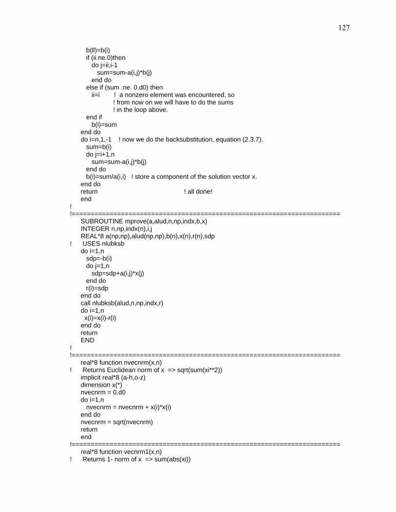
127

b(ll)=b(i) if (ii.ne.0)then do j=ii,i-1 sum=sum-a(i,j)*b(j) end do else if (sum .ne. 0.d0) then ii=i ! a nonzero element was encountered, so ! from now on we will have to do the sums ! in the loop above. end if b(i)=sum end do do i=n,1,-1 ! now we do the backsubstitution, equation (2.3.7). sum=b(i) do j=i+1,n sum=sum-a(i,j)*b(j) end do b(i)=sum/a(i,i) ! store a component of the solution vector x. end do return ! all done! end ! !======================================================================= SUBROUTINE mprove(a,alud,n,np,indx,b,x) INTEGER n,np,indx(n),i,j REAL*8 a(np,np),alud(np,np),b(n),x(n),r(n),sdp ! USES nlubksb do i=1,n sdp=-b(i) do j=1,n sdp=sdp+a(i,j)*x(j) end do r(i)=sdp end do call nlubksb(alud,n,np,indx,r) do i=1,n x(i)=x(i)-r(i) end do return END ! !======================================================================= real*8 function nvecnrm(x,n) ! Returns Euclidean norm of x => sqrt(sum(xi**2)) implicit real*8 (a-h,o-z) dimension x(*) nvecnrm = 0.d0 do i=1,n nvecnrm = nvecnrm + x(i)*x(i) end do nvecnrm = sqrt(nvecnrm) return end !======================================================================= real*8 function vecnrm1(x,n) ! Returns 1- norm of x => sum(abs(xi))

128

implicit real*8 (a-h,o-z) dimension x(*) vecnrm1 = 0.d0 do i=1,n vecnrm1 = vecnrm1 + abs(x(i)) end do return end !======================================================================= real*8 function vecnrmi(x,n) ! Returns inf norm of x => max(xi) implicit real*8 (a-h,o-z) dimension x(*) vecnrmi = 0.d0 do i=1,n temp = abs(x(I)) if (temp .gt. vecnrmi) vecnrmi = temp end do return end COMMON BLOCK DEFINITIONS

CMN_CSPEC.F character*80 c_desc character*24 psname_in, pdname_out integer kspec, ispec, jspec, kcond, kfeed real*8 fd_liq, fd_vap, fd_ctot, fd_temp, fd_pres, fd_enth, & fd_totl, fd_psi, & p, q, sd_l, sd_v, stg_mve, rxeff, totl, totv, hliq, hvap, & rxk, vlk, vars, vars0, xspec common /colspec/ fd_liq(ncmax,nsmax), fd_vap(ncmax,nsmax), & fd_ctot(ncmax,nsmax), & fd_temp(nsmax), fd_pres(nsmax), fd_enth(nsmax),fd_totl(nsmax), & fd_psi(nsmax), & p(nsmax), q(nsmax), sd_l(nsmax), sd_v(nsmax), & stg_mve(nsmax),rxeff(nsmax),holdupl(nsmax), & totl(nsmax),totv(nsmax), hliq(nsmax), hvap(nsmax), & rxk(nsmax), vlk(ncmax,nsmax), vars(0:nvmax), vars0(0:nvmax), & rxcoord, scinit, xspec(2), kspec(2), ispec(2), jspec(2), kcond, & kfeed(nsmax), psname_in, pdname_out, c_desc ! integer in_spc, out_spc, out_log, out_sol, out_pth, in_cdata common /iochn/in_spc, out_spc, out_log, out_sol, out_pth, in_cdata CMN_HSPARMS.F common /hsparms/ dir, dso, dsmin, dsmax, xmax, & ecorc, ecorb, edet, esol, ebif, etur, esta, easy, & idom, ihom, maxdet, minasy, maxasy CMN_PARAMS.F common /params/ns, nc CMN_THERMO.F character*24 cname logical kinetic common /thermo/ cname(ncmax), cmolwt(ncmax), tmelt(ncmax),

129

& tboil(ncmax), tcrit(ncmax), pcrit(ncmax), vcrit(ncmax), & zcrit(ncmax), acfac(ncmax), delhf(ncmax), delgf(ncmax), & tcpmin(ncmax), tcpmax(ncmax), cpa0(ncmax),cpa1(ncmax), & cpa2(ncmax), cpa3(ncmax), cpa4(ncmax),vpa(ncmax), vpb(ncmax), & vpc(ncmax), pvpmin(ncmax), pvpmax(ncmax), tvpmin(ncmax), & tvpmax(ncmax),rxsto(ncmax), & fwvl(ncmax), acvl, bcvl, zcvl, uvl, wvl, fuwvl, & rgas, & alpha, tb1, delhv, delhr, cpl, cpv, tref, & rxnke0, rxeeql, rxkf0, rxefwd, rxntref, & kthermo, & kinetic PGM_PARAMS.F parameter (nsmax = 50, ncmax = 10, nvmax = nsmax*(2*ncmax+2)) parameter (nimax = nvmax, nrmax = 2*nimax)

130

APPENDIX C.

REACTIVE FLASH PROGRAM SOURCE CODE

131

MAIN PROGRAM program scflash ! Distillation computation by simultaneous correction method. ! Revised main program ! Written by: T. Mills ! Date: 04/08/2009 ! ! ! Specification statements: implicit real*8 (a-h,o-z) logical c_in, f_in, dflag, quit, first, feasible, rstart integer ioflag, kthermo, nargs, nc, ns, method ! ! Set parameter values include "pgm_params.f" ! parameter (dflag = .false.) ! ! Define local storage areas integer nnull, nnullv(nvmax) real*8 tmpdfx(nvmax,nvmax), tmpfx(nvmax), tmpwrk(nvmax), solndet ! ! Define common storage areas include "cmn_params.f" include "cmn_cspec.f" include "cmn_thermo.f" ! ! Define i/o channels data in_spc,out_spc,out_log,out_sol,in_cdata/ 10,11,12,13,14/ data out_pth/ 15/ ! !----------------------------------------------------------------------- ! Executable statements begin here ! ! Get the name of the input file, then open the file if ! it exists, or quit. ! if (iargc() .ge. 1) then call getarg(1,psname_in); else write (*,'(a$)') " Problem Specification file: " read (*,*) psname_in if ( psname_in .eq. ' ') stop end if inquire(file= psname_in, exist= f_in) if (f_in) then open (in_spc, file = psname_in, status = "old" ) rewind in_spc else write (*,'(a$)') " Specification file doesn't exist... " stop end if ! first = .true. do ! while ( .not. quit) !-----------------------------------------------------------------------

132

! Get problem specification call probspec(f_in,method,first,quit) ! Exit if no new case to solve if (quit) then write (*,*) "Termination signal given" stop end if ! Open files for log and problem solutions open (out_log, file = pdname_out(1:LnBlnk(pdname_out))//'.log' ) open (out_sol, file = pdname_out(1:LnBlnk(pdname_out))//'.sol' ) open (out_pth, file = pdname_out(1:LnBlnk(pdname_out))//'.pth' ) ! !----------------------------------------------------------------------- ! Set up initial profile guesses call initprob ! !----------------------------------------------------------------------- ! Initial profiles are set, now time to solve the problem. write (*,*) write (*,*)"Case: ",pdname_out write (*,*)c_desc write (*,*) write(out_log,*)"Initial estimates..." call display(out_log) do j=1,2*nc+2 !Save initial starting point vars0(j) = vars(j) end do kstatus = 0 maxits = 5000 nsoln = 0; nturn = 0; nstart = 1; nfeas = 0; nstalls = 3 do while (.true.) call solver(vars,2*nc+2,1.d-6,1.d-06,100, & kstatus,nits,error,out_log,out_pth) write (*,*)"Homotopy parm ",error," after ",nits," steps." write (out_log,*)"Homotopy parm ",error," after ",nits, & " steps." if (kstatus .lt. 100) nstalls = 3 if (kstatus .eq. 1) then !Solution point found feasible = .true. do j=1,2*nc+2 if (j .ne. (nc+2) .and. vars(j) .lt. & -1.d-7) feasible = .false. end do call funcv(vars(1),tmpfx,2*nc+2,nnull) call fdjac(vars(1),tmpfx,tmpdfx,2*nc+2,nvmax) call ludcmp(tmpdfx,2*nc+2,nvmax,nnullv,tmpwrk,solndet, & nnull) nsoln = nsoln + 1 if (feasible) then nfeas = nfeas + 1 write (*,*) "Feasible solution ",nfeas,":" write (out_sol,*) "Feasible solution ",nfeas,":" write (out_log,*) "Feasible solution ",nfeas,":" write (*,*) "Jacobian Determinant: ",solndet write (out_sol,*) "Jacobian Determinant: ",solndet write (out_log,*) "Jacobian Determinant: ",solndet

133

! write column profiles to console for excel call display2 else write (*,*) "Infeasible solution" write (out_sol,*) "Infeasible solution:" write (out_log,*) "Infeasible solution:" write (*,*) "Jacobian Determinant: ",solndet write (out_sol,*) "Jacobian Determinant: ",solndet write (out_log,*) "Jacobian Determinant: ",solndet end if call display(out_sol) call display(out_log) kstatus = 1 else if (kstatus .eq. 2) then !Bifurcation found write (*,*) "Bifurcation found..." kstatus = 1 else if (kstatus .eq. 3) then !Trifurcation found write (*,*) "Trifurcation found..." kstatus = 1 else if (kstatus .eq. 4) then !Turning point found nturn = nturn + 1 write (*,*) "Turning point ",nturn,":" kstatus = 1 else if (kstatus .eq. 5) then !Starting point found nstart = nstart + 1 write (*,*) "Starting point ",nstart,":" rstart = .true. !test for repeated start point do j=1,2*nc+2 if (abs(vars0(j)-vars(j))/abs(vars0(j)) .ge. 1.d-6) & rstart = .false. end do if (rstart) then nstart = nstart - 1 write (*,*) "Path returns to original start point..." write (out_log,*) "returns to original start point..." exit end if kstatus = 1 else if (kstatus .eq. 10) then !Step count exceeded kstatus = 1 else if (kstatus .eq. 20 .or. kstatus .eq. 21) then ! Path goes to infinity write (*,*) "Path goes to infinity..." write (out_log,*) "Path goes to infinity..." exit else if (kstatus .eq. 101) then !Step size too small write (*,*) "Stopped due to small step size..." write (out_log,*) "Stopped due to small step size..." nstalls = nstalls - 1 if (nstalls .eq. 0) exit kstatus = 1 else if (kstatus .eq. 102) then !Process is stagnant write (*,*) "Stopped due to stagnation..." write (out_log,*) "Stopped due to stagnation..." nstalls = nstalls - 1 if (nstalls .eq. 0) exit

134

kstatus = 1 else if (kstatus .eq. 105) then !Singular homotopy matrix write (*,*) "Homotopy matrix is singular..." write (out_log,*) "Homotopy matrix is singular..." exit else if (kstatus .eq. 106) then !No tangent vector write (*,*) "Tangent vector not obtained..." write (out_log,*) "Tangent vector not obtained..." exit else if (kstatus .eq. 201) then !Start point out of bounds write (*,*) "Start point out of domain..." write (out_log,*) "Start point out of domain..." exit else if (kstatus .eq. 202) then !Base point out of bounds write (*,*) "Base point out of domain..." write (out_log,*) "Base point out of domain..." exit end if if (nits .ge. maxits) then write (*,*) "Maximum steps exceeded..." exit end if end do write (*,*) write (*,*)"Solutions: ",nsoln," Feasible: ",nfeas write (*,*)"Start points: ",nstart," Turn points: ",nturn write (*,*) write (*,*) ! close (out_log) close (out_sol) close (out_pth) ! end do ! while ( .not. quit) stop end ! !======================================================================= ! Include subroutine packages ! include "probspec.f" include "initprob.f" include "display.f" include "display2.f" include "fdjac.f" include "funcv.f" include "altthermo.f" include "homotopy.f" PROBSPEC.F subroutine probspec(f_in,method,first,quit) ! Subroutine to get problem specification from console or file ! Parameters: ! f_in logical, TRUE if input to be from file ! in_spc integer, channel # for input

135

! out_spc integer, channel # for saving problem spec ! in_cdata integer, channel # for component props file ! kstatus integer, ? ! ! Specification statements: implicit real*8 (a-h,o-z) logical f_in, c_in, dflag, quit, first, cdflag integer ioflag, kthermo, nargs, nc, ns, method character*80 ans character*24 cname_in, formula, casno, cdfile character*6 command logical P1,P2,P3,P4,P5,P6,P7,P8,P9,P10,P11,P12,P13,P14,P15,P16, & P17,P18,P21,P31 save P1,P2,P3,P4,P5,P6,P7,P8,P9,P10,P11,P12,P13,P14,P15,P16, & P17,P18,P21,P31 ! ! Set parameter values include "pgm_params.f" ! ! Define common storage areas include "cmn_params.f" include "cmn_cspec.f" include "cmn_thermo.f" include "cmn_hsparms.f" ! common /rxn/ sprxk save /hsparms/ ! quit = .true. rgas=8.314510d0 !Energy units are joules !----------------------------------------------------------------------- ! Set default values if first call if (first) then P1=.false.;P2=.false.;P3=.false.;P4=.false.;P5=.false. P6=.false.;P7=.false.;P8=.false.;P9=.false.;P10=.false. P11=.false.;P12=.false.;P13=.false.;P14=.false.;P15=.false. P16=.false.;P17=.false.;P18=.false.;P21=.false.;P31=.false. nc=0; method=1; kthermo=1 kspec=0;xspec=0.d0 pdname_out=' '; c_desc=' ' do i=1,ncmax cname(i)=' ';rxsto(i)=0.d0 end do p=0.d0;fd_pres=0.d0;fd_temp=0.d0 q=0.d0 rxeff=0.d0;holdupl=0.d0 do i=1,ncmax fd_ctot(i)=0.d0 end do rxcoord = 0.d0 scinit = 1.d0 sprxk = 0.d0 idom = 0; ihom = 1; dir = 1.d0; dso = 1.d-01 dsmin = 1.d-20; dsmax = 5.d04; xmax = 1.d05 ecorc = 1.d-04; ecorb = 1.d-06; edet = 5.d-01 esol = 1.d-04; ebif = 1.d-04; etur = 1.d-06

136

esta = 1.d-04; easy = 1.d-06; maxdet = 5 minasy = 5; maxasy = 20 first = .false. end if !----------------------------------------------------------------------- pdname_out = ' '; c_desc = ' ' !Clear filename & description P1 = .false. do read (in_spc,'(a80)',IOSTAT=ioflag) ans if (ioflag .ne. 0) exit read (ans,*) command if (command .eq. "XC") exit if (command .eq. "P1") then !Case ID string read (ans,*) command, pdname_out if (pdname_out(1:1) .eq. '"') & pdname_out=pdname_out(2:len_trim(pdname_out)) P1 = .true. else if (command .eq. "P2") then !Case Description read (ans,*) command, c_desc if (c_desc(1:1) .eq. '"') & c_desc=c_desc(2:len_trim(c_desc)) P2 = .true. else if (command .eq. "P4") then !Case Thermo model read (ans,*) command, kthermo P4 = .true. else if (command .eq. "P5") then !Case Components read (ans,*) command, nc, cdfile if (cdfile(1:1) .eq. '"') & cdfile=cdfile(2:len_trim(cdfile)) inquire (file=cdfile, exist=cdflag) if (.not. cdflag) then quit=.true.; return end if open (in_cdata, file=cdfile) do i=1,nc read (in_spc,*) cname_in rewind in_cdata !find component in database do read (in_cdata,*,IOSTAT=ioflag)icomp, cname(i), & formula, casno, cmolwt(i), tmelt(i), tboil(i), & tcrit(i), pcrit(i), vcrit(i), zcrit(i), & acfac(i), delhf(i), delgf(i), tcpmin(i), & tcpmax(i), cpa0(i), cpa1(i), cpa2(i), cpa3(i), & cpa4(i), ieq, vpa(i), vpb(i), vpc(i), & pvpmin(i), pvpmax(i), tvpmin(i), tvpmax(i) if (ioflag .ne. 0) then quit=.true.; return end if if (cname(i) .eq. cname_in) exit end do end do P5 = .true. else if (command .eq. "P8") then !Case Top spec read (ans,*) command, kspec,xspec,ispec if (kspec .ne. 1 .or. kspec .ne. 2) q=xspec P8 = .true.

137

else if (command .eq. "P10") then !Case Cond P & stg delta read (ans,*) command, p P10 = .true. else if (command .eq. "P11") then !Case Feed spec !Clear old spec kfeed=0;fd_pres=0.d0;fd_temp=0.d0 do i=1,nc fd_ctot(i)=0.d0 end do read (ans,*) command, nf read (in_spc,*)j,kfeed,fd_pres,fd_temp, & (fd_ctot(i),i=1,nc) P11 = .true. else if (command .eq. "P15") then !Case Stoich coeffs read (ans,*) command, (rxsto(i),i=1,nc) P15 = .true. else if (command .eq. "P16") then !Case Rxn effs read (ans,*) command, rxeff P16 = .true. else if (command .eq. "P18") then !Stage molar holdups read (ans,*) command, holdupl P16 = .true. else if (command .eq. "P21") then !Spec homo solver parms read (ans,*) command, nq P18 = .true. if (nq .eq. 1) read (ans,*) command, nq, dir if (nq .eq. 2) read (ans,*) command, nq, dso if (nq .eq. 3) read (ans,*) command, nq, dsmin if (nq .eq. 4) read (ans,*) command, nq, dsmax if (nq .eq. 5) read (ans,*) command, nq, xmax if (nq .eq. 6) read (ans,*) command, nq, ecorc if (nq .eq. 7) read (ans,*) command, nq, ecorb if (nq .eq. 8) read (ans,*) command, nq, edet if (nq .eq. 9) read (ans,*) command, nq, esol if (nq .eq. 10) read (ans,*) command, nq, ebif if (nq .eq. 11) read (ans,*) command, nq, etur if (nq .eq. 12) read (ans,*) command, nq, esta if (nq .eq. 13) read (ans,*) command, nq, easy if (nq .eq. 14) read (ans,*) command, nq, idom if (nq .eq. 15) read (ans,*) command, nq, ihom if (nq .eq. 16) read (ans,*) command, nq, maxdet if (nq .eq. 17) read (ans,*) command, nq, minasy if (nq .eq. 18) read (ans,*) command, nq, maxasy else if (command .eq. "P31") then !input for simple thermo read (ans,*)command,alpha,tb1,delhv,delhr,cpl,cpv, & rxntref, rxnke0,rxkf0,rxefwd kinetic = .true. !default to kinetic reaction model xtemp=0.d0 !set up to allocate delhr do i=1,nc if (rxsto(i) .gt. 0.d0) xtemp=xtemp+rxsto(i) end do do i=1,nc cpa0(i)=cpl; cpa1(i)=cpv; delhf(i)=0.d0 if (i .eq. 1) then !set component boiling points tboil(i)=tb1 else

138

tboil(i)=delhv/(delhv/tboil(i-1) - rgas*log(alpha)) end if vpb(i) = delhv / rgas vpa(i) = 1.3163d-02 + vpb(i) / tboil(i) if (rxsto(i) .gt. 0.d0) delhf(i)=delhr*rxsto(i)/xtemp end do rxeeql = delhr !set constants for rxn equilibrium K if (rxkf0 .eq. 0.d0) kinetic = .false. else if (command .eq. "P32") then !input for Antoine eq read (ans,*)command,i,vpa(i),vpb(i) tboil(i) = vpb(i) / ( vpa(i) - 1.3163d-02) else if (command .eq. "P33") then !rx coord for init read (ans,*)command,rxcoord else if (command .eq. "P34") then !scale factor for init read (ans,*)command,scinit end if end do ! ! Determine whether or not to run a case quit = .not. (P1 .and. P5 .and. P8 .and. P10 .and. P11) ! return end INITPROB.F subroutine initprob ! Subroutine to set up initial solution estimates ! ! ! Specification statements: implicit real*8 (a-h,o-z) logical c_in, dflag, quit, trefset integer ioflag, kthermo, nargs, nc, ns character*80 ans character*24 cname_in, formula, casno ! ! Set parameter values include "pgm_params.f" ! parameter (dflag = .false.) ! ! Define local storage areas real*8 xnull, fvnull(ncmax),flnull(ncmax) real*8 zfeed(ncmax), xfeed(ncmax), yfeed(ncmax),fctotal(ncmax), & rxlim(ncmax),bulk_l(nsmax),bulk_v(nsmax), & f(nsmax),g(ncmax,nsmax),vlek(ncmax,nsmax), & fvalues(0:nvmax),fftf,ffvf ! ! Define common storage areas include "cmn_params.f" include "cmn_cspec.f" include "cmn_thermo.f" ! common /rxn/ sprxk ! !------------------------------------------ ! Clear the feed variables

139

ffvf=0.d0; fftf=0.d0 tref=tboil(1) fd_enth=0.d0; fd_totl=0.d0; fd_psi=0.d0 do i=1,nc fd_liq(i)=0.d0; fd_vap(i)=0.d0 fctotal(i) = 0.d0 end do ! ! Flash the feed, or compute its temperatures call flash(kfeed,fd_ctot,fd_temp,fd_pres,p, & xfeed,yfeed,fd_enth,fd_totl,fd_psi) do i=1,nc fd_liq(i) = xfeed(i) fd_vap(i) = yfeed(i) ffvf = ffvf + yfeed(i) fctotal(i) = fctotal(i) + fd_ctot(i) fftf = fftf + fd_ctot(i) end do ffvf = ffvf / fftf !Fraction of total feed as vapor ! ! React composite feed to start if (rxcoord .ge. 0.d0 .and. rxcoord .le. 1.d0) then !Reaction coordinate is specified do i=1,nc !Compute feed over stoich coeff for all cpds rxlim(i) = 0.d0 if(rxsto(i) .ne. 0.d0) rxlim(i) = -fctotal(i)/rxsto(i) end do rxflim = 0.d0; rxblim = 0.d0 do i=1,nc !find limiting extents rxblim = min(rxblim,rxlim(i)) rxflim = max(rxflim,rxlim(i)) end do do i=1,nc if (rxsto(i) .gt. 0) rxblim = max(rxblim,rxlim(i)) if (rxsto(i) .lt. 0) rxflim = min(rxflim,rxlim(i)) end do rxext = rxcoord*(rxflim - rxblim) + rxblim !Reaction extent else !Approach to equilibrium is specified if (rxcoord .ge. 1.d0 .or. rxcoord .le. -1.d0) rxcoord = -1.d0 !limit values to 0>x>=-1 call flash(4,fctotal,fd_temp,p,p, & flnull,fvnull,xnull,xnull,ffvf) !Est avg T rxext = rxex(fctotal,fd_temp,p,nc,0,0) !Reaction extent rxext = -rxcoord * rxext end if fctsum = 0.d0 do i=1,nc fctotal(i) = fctotal(i) + rxsto(i)*rxext fctsum = fctsum + fctotal(i) !sum of reacted feed end do do i=1,nc fctotal(i) = fctotal(i)/fctsum !convert to mol fractions end do ! ! Set initial reaction extent estimates

140

vars(nc+2) = 0.d0 ! ! Set initial temperature estimate vars(nc+1) = fd_temp if (kspec .eq. 2) vars(nc+1) = xspec ! ! Approximate D/F and L1/D fdf = fd_psi !D/F if (kspec .eq. 1) fdf = xspec if (fdf .eq. 0.d0) fdf = 1.d-05 !Need at least some vapor to start fld = 1.d0 - fdf !L/D ! ! Tref = avg temperature tref = vars(nc+1) ! ! Set bulk flow profiles, assuming constant overflow totv = fdf * fctsum !D totl = fld * fctsum !L ! ! Set component flow profiles jv=0; jl=jv+nc+2 do i=1,nc vars(jv+i) = totv * fctotal(i) * scinit vars(jl+i) = totl * fctotal(i) * scinit end do ! return end DISPLAY.F subroutine display(kchnl) ! Write distillation problem/solution description to console or ! log file. ! ! INPUTS: ! kchnl: i/o channel to use for output ! implicit real*8 (a-h,o-z) include "pgm_params.f" !Program parameters include "cmn_params.f" !No. stages and No. components include "cmn_cspec.f" !Column specifications include "cmn_thermo.f" !Thermodynamic data ! common /rxn/ sprxk real*8 xtemp(ncmax) ! !----------------------------------------------------------------------- ! Show case ID and Description write (kchnl,*) write (kchnl,*)"Case ID: ", pdname_out write (kchnl,'(a)')c_desc ! !----------------------------------------------------------------------- ! Show thermodynamic model used ! write (kchnl,'(a$)')"Thermodynamic model: " ! if (kthermo .eq. 4) then

141

! write (kchnl,'(a)')"Van der Waals" ! else if (kthermo .eq. 3) then ! write (kchnl,'(a)')"Redlich-Kwong" ! else if (kthermo .eq. 2) then ! write (kchnl,'(a)')"Soave-Redlich-Kwong" ! else ! write (kchnl,'(a)')"Peng-Robinson" ! end if ! !----------------------------------------------------------------------- ! Show no. stages, no. components, and condenser type write (kchnl,'(a,i3)')" Components: ",nc ! if (kcond .eq. 2) then ! write (kchnl,'(a)')"Partial" ! else ! write (kchnl,'(a)')"Total" ! end if ! !----------------------------------------------------------------------- ! Show component data (simplified system) write(kchnl,'(a)')"Component information:" write(kchnl,'(a)')" alpha Hv Hr"// &" CpL CpV Krx" write(kchnl,'(8x,6f10.2)')alpha,delhv,delhr,cpl,cpv,rxnke0 write(kchnl,'(a)')" nu Tb CpL"// &" CpV Hr" do i=1,nc write(kchnl,'(2x,a6,5f10.2)')cname(i),rxsto(i),tboil(i),cpa0(i), & cpa1(i),delhf(i) end do ! !----------------------------------------------------------------------- ! Show material balance and energy balance specifications if (kspec .eq. 1) then !Spec V/F write(kchnl,'(a,f10.3)')"Specified Vapor Fraction:",xspec else if (kspec .eq. 2) then !Spec T write(kchnl,'(a,f10.3)')"Specified Temperature:",xspec end if ! !----------------------------------------------------------------------- ! Show column feeds write(kchnl,*)"Feed:" write(kchnl,1010)"Temp(K): ",fd_temp, & " Press(bar): ",fd_pres, & " Enthalpy(J): ",fd_enth 1010 format(a,f9.4,a,f9.4,a,f9.2) write(kchnl,*)" "," Liquid Vapor" do i=1,nc write(kchnl,'(a12,2f10.4)')cname(i),fd_liq(i), fd_vap(i) end do ! !----------------------------------------------------------------------- ! Show Heat duty. qc = (- fd_enth & + hstream(vars(1),vars(nc+1),p,nc,1) & + hstream(vars(nc+3),vars(nc+1),p,nc,0))

142

& /1.d3 write(kchnl,*)"Heat duty(kJ): ",qc ! !----------------------------------------------------------------------- ! Show pressure, temperature, heat duty, side draw, and ! efficiency profiles write(kchnl,'(a)')" Q(kJ) "// & "Rxn eff Rx(mol) Rx(kJ)" do i=1,nc xtemp(i)=fd_liq(i)+fd_vap(i)-vars(i) end do rxx = rxex(xtemp,vars(nc+1),p,nc,0,0)* rxeff write (kchnl,1000)q,rxeff,rxx,rxx*delhr/1.d3 1000 format(2x,7f11.4) ! !----------------------------------------------------------------------- ! Show Pressure, Temperature, Heat duty, and Bulk flow profiles. write(kchnl,'(a)')" P(bar) T(K) "// & "L(mol) V(mol) H err L(kJ) V(kJ)" jstg = 0 totv = 0.d0 totl = 0.d0 do i=1,nc totv = totv + vars(jstg+i) totl = totl + vars(jstg+nc+2+i) vlk(i) = vler(vars(jstg+nc+3),vars(jstg+1), & vars(jstg+nc+1),p,nc,i) end do hvap = hstream(vars(jstg+1),vars(jstg+nc+1),p,nc,1)/ 1.d3 hliq = hstream(vars(jstg+nc+2+1),vars(jstg+nc+1),p,nc,0)/ 1.d3 rxk = rxer(vars(jstg+nc+3),vars(jstg+nc+1),p,nc,0,0) herr = fd_enth+q-hliq-hvap if (q .eq. 0.d0) herr = herr + qc write (kchnl,1000)p,vars(jstg+nc+1),totl,totv, herr,hliq,hvap write (kchnl,'(57x,2f11.4)')hliq/totl,hvap/totv !----------------------------------------------------------------------- ! Show Vapor flow profiles write(kchnl,*)"Vapor flows/compositions:" do ii=1,nc,5 ij=ii+4 if (ij .ge. nc) ij=nc write(kchnl,'(6x,5a12)')(cname(i),i=ii,ij) jj=0 write(kchnl,'(2x,5f12.4)')(vars(jj+i),i=ii,ij) write(kchnl,'(2x,5f12.6)')(vars(jj+i)/totv,i=ii,ij) end do ! !----------------------------------------------------------------------- ! Show Liquid flow profiles write(kchnl,*)"Liquid flows/compositions:" do ii=1,nc,5 ij=ii+4 if (ij .ge. nc) ij=nc write(kchnl,'(6x,5a12)')(cname(i),i=ii,ij) jj=nc+2 write(kchnl,'(2x,5f12.4)')(vars(jj+i),i=ii,ij)

143

write(kchnl,'(2x,5f12.6)')(vars(jj+i)/totl,i=ii,ij) end do ! !----------------------------------------------------------------------- ! Show component creation/consumption write(kchnl,*)"Component creation & consumption:" do i=1,nc xtemp(i)=vars(i)+vars(nc+2+i) xtemp(i)=xtemp(i)-fd_liq(i)-fd_vap(i) end do do ii=1,nc,5 ij=ii+4 if (ij .ge. nc) ij=nc write(kchnl,'(6x,5a12)')(cname(i),i=ii,ij) write(kchnl,'(2x,5f12.4)')(xtemp(i),i=ii,ij) end do ! !----------------------------------------------------------------------- ! Show VLE equilibrium ratios write(kchnl,*)"Vapor/Liquid equilibrium ratios:" do ii=1,nc,5 ij=ii+4 if (ij .ge. nc) ij=nc write(kchnl,'(9x,5a12)')(cname(i),i=ii,ij) jv=0 jl=jv+nc+2 write(kchnl,'(2x,5e12.4)')(vlk(i),i=ii,ij) write(kchnl,'(5x,5e12.4)')(((vars(jv+i)*totl)/ & (vars(jl+i)*totv)),i=ii,ij) end do ! !----------------------------------------------------------------------- ! Show Reaction equilibrium ratios write(kchnl,*)"Reaction equilibrium ratios:" write(kchnl,'(3x,a,2x,a)')"From thermo","From flows" rktemp = 1.d0 do i=1,nc if (rxsto(i) .ne. 0.d0) rktemp=rktemp* & ((vars(nc+2+i)/totl)**rxsto(i)) end do write(kchnl,'(2x,2e12.4)')rxk,rktemp ! !----------------------------------------------------------------------- ! Show Stream bubble and dew points write (kchnl,*)"Stream bubble/dew points:" write (kchnl,*)" L bubble V dew" jstg=0 dbub=bubpt(vars(jstg+nc+3),p) ddew=dewpt(vars(jstg+1),p) write(kchnl,'(2x,2f10.4)')dbub,ddew return end DISPLAY2.F subroutine display2

144

! Write solution description to console for excel ! implicit real*8 (a-h,o-z) include "pgm_params.f" !Program parameters include "cmn_params.f" !No. stages and No. components include "cmn_cspec.f" !Column specifications include "cmn_thermo.f" !Thermodynamic data ! real*8 xtemp(ncmax) ! !----------------------------------------------------------------------- ! Show case ID write (*,*) write (*,*)"Case ID,", pdname_out ! !----------------------------------------------------------------------- ! Show Temperature and Bulk flow profiles. write(*,*)"j,T,L,V,L/V" jstg = 0 totv = 0.d0 totl = 0.d0 do i=1,nc totv = totv + vars(jstg+i) totl = totl + vars(jstg+nc+2+i) end do jstg = 0 write (*,'(f12.6,3(",",f12.6))')vars(jstg+nc+1),totl, & totv,totl/totv !----------------------------------------------------------------------- ! Show Vapor composition profiles write(*,*)"y's" jstg = 0 write(*,'(f12.6,9(",",f12.6))')(vars(jstg+i)/totv,i=1,nc) ! !----------------------------------------------------------------------- ! Show Liquid composition profiles write(*,*)"x's" jstg = nc+2 write(*,'(f12.6,9(",",f12.6))')(vars(jstg+i)/totl,i=1,nc) ! !----------------------------------------------------------------------- ! Show component overall conversion write(*,*)"Overall conversion" do i=1,nc xtemp(i)=fd_ctot(i) if (xtemp(i) .ne. 0.d0) xtemp(i)=1.d0- & ((vars(i)+vars(nc+2+i))/xtemp(i)) end do write(*,'(f12.6,9(",",f12.6))')(xtemp(i),i=1,nc) ! !----------------------------------------------------------------------- ! Show Condenser and Reboiler duties. qc = (- fd_enth & + hstream(vars(1),vars(nc+1),p,nc,1) & + hstream(vars(nc+3),vars(nc+1),p,nc,0)) & /1.d3

145

write(*,*)"Heat duty(kJ),",qc ! !----------------------------------------------------------------------- return end FDJAC.F subroutine fdjac(x,fvec,df,n,NP) ! USES funcv implicit real*8 (a-h,o-z) PARAMETER (EPS=1.d-5) dimension df(np,np),fvec(np),x(np),f(np) ! Computes forward-difference approximation to Jacobian. On input, ! x(1:n) is the point at which the Jacobian is to be evaluated, ! fvec(1:n) is the vector of function values at the point, and np ! is the physical dimension of the Jacobian array df(1:n,1:n) which ! is output. subroutine funcv(n,x,f) is a fixed-name, user-supplied ! routine that returns the vector of functions at x. ! Parameters: EPS is the approximate square root of the machine ! precision. do j=1,n temp=x(j) h=EPS*abs(temp) if(h .eq. 0.d0)h=EPS x(j)=temp+h !Trick to reduce finite precision error. h=x(j)-temp call funcv(x, f, n, ierr) x(j)=temp do i=1,n !Forward difference formula. df(i,j)=(f(i)-fvec(i))/h end do end do return end FUNCV.F subroutine funcv(x,f,n,ierr) ! Calculate discrepancy function values f, for the column ! variables held in vector x. ! REVISED: 4/8/09 Changed column to flash drum ! INPUTS: ! x : vector of column variables, as follows for each ! stage - nc vapor flows, 1 stage temperature, 1 stage ! reaction extent, and nc liquid flows. ! n : number of equations to evaluate - not used in this ! implementation. ! OUTPUTS: ! f : vector of calculated discrepancy function values - ! for each stage 1 energy balance, 1 reaction ! equilibrium function, nc material balances, ! and nc equilibrium relationships. ! ierr: error flag ( >0 if error) ! implicit real*8 (a-h,o-z) include "pgm_params.f"

146

include "cmn_params.f" include "cmn_cspec.f" include "cmn_thermo.f" ! real*8 x(*),f(*) real*8 xt(ncmax) !vector of stage l-primes ! jxv = 0 !pointer to vapor flows jxt = jxv+nc+1 !Pointer to temperature jxx = jxt+1 !Pointer to rxn extent jxl = jxx !pointer to liquid flows jfe = 1 !pointer to energy bal function jfr = jfe+1 !pointer to rxn eq function jfm = jfr !pointer to matl bal functions jfq = jfm+nc !pointer to v/l equil functions ! ! calculate total stage flows tlj = 0.d0; tvj = 0.d0 xmaxl = 0.d0; imaxl = 0 xtsum = 0.d0; eps = 0.d0 do i=1,nc tlj = tlj + x(jxl+i) tvj = tvj + x(jxv+i) xt(i) = fd_liq(i) + fd_vap(i) - x(jxv+i) if (x(jxl+i) .ge. xmaxl)then xmaxl = x(jxl+i) imaxl = i end if xtsum = xtsum + xt(i); eps = eps + rxsto(i) end do ! do i=1,nc ! Material Balance Functions f(jfm+i)= -fd_ctot(i)-x(jxx)*rxsto(i)+x(jxv+i)+x(jxl+i) ! ! Vapor / Liquid Equilibrium functions vk = vler(x(jxl+1),x(jxv+1),x(jxt),p,nc,i) !VLE K f(jfq+i) = vk*x(jxl+i)/tlj - x(jxv+i)/tvj ! f(jfq+i) = f(jfq+i)*(tlj+tvj)/2.d0 !Scale to M functions end do ! ! Energy balance function f(jfe) = -q - fd_enth & +hstream(x(jxl+1),x(jxt),p,nc,0) & +hstream(x(jxv+1),x(jxt),p,nc,1) !Scale H functions to M's ! f(jfe) = f(jfe)/((hstream(x(jxl+1),x(jxt),p,nc,0)/tlj+ ! & hstream(x(jxv+1),x(jxt),p,nc,1)/tvj)/2) ! ! Reaction equilibrium function rxk = rxer(xt,x(jxt),p,nc,i,0) if ((kinetic .and. holdupl .eq. 0.d0) .or. (.not. kinetic & .and. rxeff .eq. 0.d0))then f(jfr) = x(jxx) - 0.d0 !no reaction else if (kinetic) then !kinetic reaction model

147

rxneff = 1.d0; rxntot = xtsum+rxneff*eps*x(jxx) f2 = holdupl*rxkf(xt,x(jxt),p,nc,i,0)/rxntot f1 = rxk*f2; f3 = rxk*x(jxx)/rxntot else !equilibrium reaction model rxneff = 1.d0/rxeff; rxntot = xtsum+rxneff*eps*x(jxx) f1 = rxk; f2 = 1.d0; f3 = 0.d0 end if do i=1,nc if (rxsto(i) .lt. 0.d0) then f1 = f1 * ((xt(i)+(rxneff*rxsto(i)*x(jxx)))/ & rxntot)**(-rxsto(i)) else if (rxsto(i) .gt. 0.d0) then f2 = f2 * ((xt(i)+(rxneff*rxsto(i)*x(jxx)))/ & rxntot)**rxsto(i) end if end do f(jfr) = f1 - f2 - f3 end if ! ! Substitute functions due to specifications ! if (kspec .eq. 1) then !Spec V/F dst = 0.d0 do i=1,nc dst = dst + x(jxv+i) end do f(jfe) = dst - xspec*fd_totl else if (kspec .eq. 2) then !Spec T f(jfe) = x(jxt) - xspec end if ierr = 0 ! return end ALTTHERMO.F subroutine flash(kf, zf, tf, pf, pstg, xf, yf, hf,ftotal,psi) ! Computes the flash of stream zf to form streams xf and yf ! Inputs: ! kf : flash type ! zf : vector containing feed compositions or flows ! tf : flash temperature ! pf : flash pressure ! pstg: ? ! Outputs: ! xf : vector of output liquid compositions or flows ! yf : vector of output vapor compositions or flows ! hf : ! ftotal: ! psi : Fraction of feed leaving as vapor ! ! Specification statements: implicit real*8 (a-h,o-z) ! Set parameter values include "pgm_params.f"

148

parameter (itmax = 25, xacc = 1.d-6) ! Define data storage include "cmn_params.f" real*8 zf(ncmax), xf(ncmax), yf(ncmax), z(ncmax), x(ncmax), & y(ncmax), vlek(ncmax), ftotal, psi, tbp, tdp fpsi(psi, i) = z(i)*(1.d0-vlek(i))/(1.d0+psi*(vlek(i)-1.d0)) ftmp(t,i) = z(i)*(1.d0-vler(z,z,t,pstg,nc,i))/ & (1.d0+psi*(vler(z,z,t,pstg,nc,i)-1.d0)) ! ! Normalize feed vector and calculate dew and bubble points ftotal = 0.d0 do i=1,nc ftotal = ftotal + zf(i) end do do i=1,nc z(i) = zf(i)/ftotal; x(i) = 0.d0; y(i) = 0.d0 end do tbp = bubpt(z, pstg) tdp = dewpt(z, pstg) if (kf .eq. 1) then ! Bubble point liquid feed tf = tbp hf=hstream(zf,tf,pf,nc,0) do i=1,nc xf(i) = zf(i); yf(i) = 0.d0 end do psi = 0.d0 else if (kf .eq. 2) then ! Dew point vapor feed tf = tdp hf=hstream(zf,tf,pf,nc,1) do i=1,nc yf(i) = zf(i); xf(i) = 0.d0 end do psi = 1.d0 else if (kf .eq. 3) then ! Spec temp flash if (tf .ge. tdp) then !T above dew point do i=1,nc yf(i) = zf(i); xf(i) = 0.d0 end do psi = 1.d0 hf=hstream(zf,tf,pf,nc,1) else if (tf .le. tbp) then !T below bubble point do i=1,nc xf(i) = zf(i); yf(i) = 0.d0 end do psi = 0.d0 hf=hstream(zf,tf,pf,nc,0) else !T between dew & bubble pts psi1 = 0.d0 psi2 = 1.d0 f1 = 0.d0 f2 = 0.d0 psi = -1 do i=1,nc vlek(i) = vler(z,z,tf,pstg,nc,i) f1 = f1 + fpsi(psi1, i)

149

f2 = f2 + fpsi(psi2, i) end do do n=1,itmax psi3 = 0.5d0*(psi1+psi2) f3 = 0.d0 do i=1,nc f3 = f3 + fpsi(psi3, i) end do psi4 = psi3 + (psi3 - psi1)*(sign(1.d0, f1-f2)*f3 & /sqrt(f3**2 - f1*f2)) if (abs(psi4-psi) .le. xacc) then exit end if psi = psi4 f4 = 0.d0 do i=1,nc f4 = f4 + fpsi(psi4, i) end do if (f4 .eq. 0.d0) then end if if (sign(f3, f4) .ne. f3) then psi1 = psi3; f1 = f3; psi2 = psi4; f2 = f4 else if (sign(f1, f4) .ne. f1) then psi2 = psi4; f2 = f4 else if (sign(f2, f4) .ne. f2) then psi1 = psi4; f1 = f4 end if end do do i=1,nc x(i) = z(i) / (1.d0+psi*(vlek(i)-1.d0)) y(i) = x(i)*vlek(i) xf(i) = ftotal * (1.d0-psi) * x(i) yf(i) = ftotal * psi *y(i) end do hf=psi*hstream(zf,tf,pf,nc,1) + & (1.d0-psi)*hstream(zf,tf,pf,nc,0) end if else if (kf .eq. 4) then !Spec V/F flash if (psi .le. 0.d0) then !All liquid do i=1,nc xf(i) = zf(i); yf(i) = 0.d0 end do tf = tbp hf = hstream(zf,tf,pf,nc,0) else if (psi .ge. 1.d0) then !All vapor do i=1,nc yf(i) = zf(i); xf(i) = 0.d0 end do tf = tdp hf = hstream(zf,tf,pf,nc,1) else t1 = tbp; f1 = 0.d0 t2 = tdp; f2 = 0.d0 tf = -1.d0 do i=1,nc f1 = f1+ftmp(t1,i)

150

f2 = f2+ftmp(t2,i) end do do n=1,itmax t3 = 0.5d0*(t1+t2); f3 = 0.d0 do i=1,nc f3 = f3+ftmp(t3,i) end do t4 = t3 + (t3-t1)*(sign(1.d0,f1-f2)*f3 & /sqrt(f3**2 - f1*f2)) if (abs(t4-tf) .le. xacc) then exit end if tf = t4; f4 = 0.d0 do i=1,nc f4 = f4+ftmp(t4,i) end do if (f4 .eq. 0.d0) then end if if (sign(f3,f4) .ne. f3)then t1 = t3; f1 = f3; t2 = t4; f2 = f4 else if (sign(f1,f4) .ne. f1) then t2 = t4; f2 = f4 else if (sign(f2,f4) .ne. f2) then t1 = t4; f1 = f4 end if end do do i=1,nc vlek(i) = vler(z,z,tf,pstg,nc,i) x(i) = z(i) / (1.d0+psi*(vlek(i)-1.d0)) y(i) = x(i) * vlek(i) xf(i) = ftotal * (1.d0-psi) * x(i) yf(i) = ftotal * psi * y(i) end do hf = psi*hstream(zf,tf,pf,nc,1) + & (1.d0-psi)*hstream(zf,tf,pf,nc,0) end if end if return end !======================================================================= real*8 function bubpt(x,p) ! Computes bubblepoint temperature of stream x at pressure p ! ! Specification statements: implicit real*8 (a-h,o-z) ! Set parameter values include "pgm_params.f" parameter (itmax = 50, xacc = 1.d-6, factor = 1.6d0) ! Define data storage include "cmn_params.f" include "cmn_thermo.f" ! real*8 x(ncmax),xnorm(ncmax) ! ! Normalize x xnormsum=0.d0

151

do i=1,nc xnormsum=xnormsum+x(i) end do do i=1,nc xnorm(i)=x(i)/xnormsum end do ! Use component boil points to start t1 = tboil(1) t2 = tboil(nc) f1 = 1.d0 f2 = 1.d0 bubpt = -1.d0 do i=1,nc f1 = f1 - xnorm(i) * vler(xnorm,xnorm,t1,p,nc,i) f2 = f2 - xnorm(i) * vler(xnorm,xnorm,t2,p,nc,i) end do do n=1,itmax ! make sure point is bracketed if (f1*f2 .lt. 0.d0) exit if (abs(f1) .lt. abs(f2)) then t1 = t1+factor*(t1-t2) f1 = 1.d0 do i=1,nc f1 = f1 - xnorm(i) * vler(xnorm,xnorm,t1,p,nc,i) end do else t2 = t2+factor*(t2-t1) f2 = 1.d0 do i=1,nc f2 = f2 - xnorm(i) * vler(xnorm,xnorm,t2,p,nc,i) end do end if end do if (f1*f2 .ge. 0.d0) write(*,*)"BUBPT: Failed to find range." do n=1,itmax ! search for best value t3 = 0.5d0*(t1+t2) f3 = 1.d0 do i=1,nc f3 = f3 - xnorm(i) * vler(x,x,t3,p,nc,i) end do t4 = t3 + (t3 - t1)*(sign(1.d0, f1-f2)*f3/sqrt(f3**2 - f1*f2)) if (abs(t4-bubpt) .le. xacc) return bubpt = t4 f4 = 1.d0 do i=1,nc f4 = f4 - xnorm(i) * vler(x,x,t4,p,nc,i) end do if (f4 .eq. 0.d0) return if (sign(f3, f4) .ne. f3) then t1 = t3; f1 = f3; t2 = t4; f2 = f4 else if (sign(f1, f4) .ne. f1) then t2 = t4; f2 = f4 else if (sign(f2, f4) .ne. f2) then t1 = t4; f1 = f4 end if if (abs(t2 - t1) .le. xacc) return

152

end do write (*,*) "BUBPT: fails to converge in ",itmax," iterations" write(*,*)"BUBPT: Returned value is: ",bubpt return end !======================================================================= real*8 function dewpt(x,p) ! Computes dewpoint temperature of stream x at pressure p ! ! Specification statements: implicit real*8 (a-h,o-z) ! Set parameter values include "pgm_params.f" parameter (itmax = 50, xacc = 1.d-6, factor = 1.6d0) ! Define data storage include "cmn_params.f" include "cmn_thermo.f" ! real*8 x(ncmax),xnorm(ncmax) ! ! Normalize x xnormsum=0.d0 do i=1,nc xnormsum=xnormsum+x(i) end do do i=1,nc xnorm(i)=x(i)/xnormsum end do ! Use component boil points to start t1 = tboil(1) t2 = tboil(nc) f1 = 1.d0 f2 = 1.d0 dewpt = -1.d0 do i=1,nc f1 = f1 - xnorm(i) / vler(xnorm,xnorm,t1,p,nc,i) f2 = f2 - xnorm(i) / vler(xnorm,xnorm,t2,p,nc,i) end do do n=1,itmax ! make sure point is bracketed if (f1*f2 .lt. 0.d0) exit if (abs(f1) .lt. abs(f2)) then t1 = t1+factor*(t1-t2) f1 = 1.d0 do i=1,nc f1 = f1 - xnorm(i) / vler(xnorm,xnorm,t1,p,nc,i) end do else t2 = t2+factor*(t2-t1) f2 = 1.d0 do i=1,nc f2 = f2 - xnorm(i) / vler(xnorm,xnorm,t2,p,nc,i) end do end if end do if (f1*f2 .ge. 0.d0) write(*,*)"DEWPT: Failed to find range."

153

do n=1,itmax ! search for best value t3 = 0.5d0*(t1+t2) f3 = 1.d0 do i=1,nc f3 = f3 - xnorm(i) / vler(xnorm,xnorm,t3,p,nc,i) end do t4 = t3 + (t3 - t1)*(sign(1.d0, f1-f2)*f3/sqrt(f3**2 - f1*f2)) if (abs(t4-dewpt) .le. xacc) return dewpt = t4 f4 = 1.d0 do i=1,nc f4 = f4 - xnorm(i) / vler(xnorm,xnorm,t4,p,nc,i) end do if (f4 .eq. 0.d0) return if (sign(f3, f4) .ne. f3) then t1 = t3; f1 = f3; t2 = t4; f2 = f4 else if (sign(f1, f4) .ne. f1) then t2 = t4; f2 = f4 else if (sign(f2, f4) .ne. f2) then t1 = t4; f1 = f4 end if if (abs(t2 - t1) .le. xacc) return end do write (*,*) "DEWPT: fails to converge in ",itmax," iterations" write(*,*)"DEWPT: Returned value is: ",dewpt return end !======================================================================= real*8 function rxex(x,t,pstg,nc,ic,kst) ! Compute the equilibrium extent of reaction at t and p ! Inputs: ! x : vector of stream compositions or flows ! t : temperature for the calculation, K ! p : pressure for the calculation, bar ! nc : number of components in x ! ic : component index (not used in this calc'n) ! kst: Stream state (0=>liquid; 1=>vapor) ! Outputs: ! rxex: Calculated extent of reaction ! implicit real*8 (a-h,o-z) include "pgm_params.f" !Storage allocation parameters include "cmn_thermo.f" !component thermodynamic data dimension x(*) parameter (gs = 0.381966011d0) !parm for golden section search ! rxek = rxer(x,t,pstg,nc,ic,kst) !Get the equilibrium constant xmax = 1.d20 xmin = -1.d20 xsum = 0.d0 eps = 0.d0 do i=1,nc !find max fwd and rev extents xsum = xsum + x(i) eps = eps + rxsto(i) if (rxsto(i) .ne. 0.d0) then xtemp = - x(i) / rxsto(i)

154

if (rxsto(i) .lt. 0.d0 .and. xtemp .lt. xmax) xmax = xtemp if (rxsto(i) .gt. 0.d0 .and. xtemp .gt. xmin) xmin = xtemp end if end do ! Initialize for Brent method search to find the root a = xmin; b = xmax fa1 = 1.d0; fa2 = rxek fb1 = 1.d0; fb2 = rxek do i=1,nc !f(x) = product of factor, minus rxek if (rxsto(i) .gt. 0.d0) then fa1=fa1*((x(i)+rxsto(i)*a)/(xsum+eps*a))**rxsto(i) fb1=fb1*((x(i)+rxsto(i)*b)/(xsum+eps*b))**rxsto(i) else if (rxsto(i) .lt. 0.d0) then fa2=fa2*((x(i)+rxsto(i)*a)/(xsum+eps*a))**(-rxsto(i)) fb2=fb2*((x(i)+rxsto(i)*b)/(xsum+eps*b))**(-rxsto(i)) end if end do fa=fa1-fa2; fb=fb1-fb2 ! fa=fa-rxek; fb=fb-rxek c = b; fc = fb do k=1,100 !search loop if (fb*fc .ge. 0.d0) then ! Rename a,b,&c and adjust bounding interval d c=a; fc=fa; d=b-a; e=d end if if (abs(fc) .lt. abs(fb)) then !swap a and c with b a=b; b=c; c=a fa=fb; fb=fc; fc=fa end if tol1 = 2.d0*1.d-8*abs(b) + 0.5d0*1.d-8 !check convergence xm = 0.5d0*(c-b) if (abs(xm) .le. tol1 .or. fb .eq. 0.d0) then !Converged rxex = b return end if if (abs(e) .gt. tol1 .and. abs(fa) .gt. abs(fb)) then ! Try inverse quadratic interpolation s = fb/fa if (a .eq. c) then p = 2.d0*xm*s q = 1.d0 - s else q = fa/fc r = fb/fc p = s*(2.d0*xm*q*(q-r)-(b-a)*(r-1.d0)) q = (q-1.d0)*(r-1.d0)*(s-1.d0) end if if (p .gt. 0.d0) q = -q !Check whether in bounds p = abs(p) if (2.d0*p .lt. min(3.d0*xm*q-abs(tol1*q), abs(e*q))) then e=d !Accept interpolation d=p/q else d=xm !Interpolation failed, use bisection e=d end if

155

else d=xm !Bounds decreasing too slowly, use bisection e=d end if a=b !Move last guess to a fa=fb if (abs(d) .gt. tol1) then !Evaluate new trial root b=b+d else b=b+sign(tol1,xm) end if fb1=1.d0; fb2=rxek !Compute function value for new trial root do i=1,nc if (rxsto(i) .gt. 0.d0) then fb1 = fb1*((x(i)+rxsto(i)*b)/(xsum+eps*b))**rxsto(i) else if (rxsto(i) .lt. 0.d0) then fb2 = fb2*((x(i)+rxsto(i)*b)/(xsum+eps*b))**(-rxsto(i)) end if end do fb=fb1-fb2 end do rxex = b write (*,*)"Reaction extent = ",rxex," Excess Iterations" return end !======================================================================= real*8 function vler(x,y,t,p,nc,ic) ! Computes the vapor-liquid equilibrium ratio for ! component ic in the mixture x at t and p ! Inputs: ! x : vector of liquid stream compositions or flows ! y : vector of vapor stream compositions or flows ! t : temperature for the calculation, K ! p : pressure for the calculation, bar ! nc : number of components in x ! ic : index of the component of interest ! Outputs: ! vler: Calculated value of the property ! implicit real*8 (a-h,o-z) include "pgm_params.f" !Storage allocation parameters include "cmn_thermo.f" !component thermodynamic data dimension x(*),y(*) ! vler = exp( vpa(ic) - vpb(ic)/t ) / p ! vler =exp(-((1.d0/t)-(1.d0/tboil(ic)))*delhv/rgas) return end !======================================================================= real*8 function hstream(x,t,p,nc,kst) ! Compute the enthalpy of stream x at t and p in state kst, ! relative to tref. Value returned is in units of kJ ! Inputs: ! x : vector of stream compositions or flows ! t : temperature for the calculation, K ! p : pressure for the calculation, bar

156

! nc : number of components in x ! kst: Stream state (0=>liquid; 1=>vapor) ! Outputs: ! hstream: Calculated enthalpy, kJ ! implicit real*8 (a-h,o-z) include "pgm_params.f" !Storage allocation parameters include "cmn_thermo.f" !component thermodynamic data dimension x(*) ! t0 = tref !Reference Temp hstream = 0.d0 xsum = 0.d0 do i=1,nc xsum = xsum+x(i) end do if (kst .eq. 0) then do i=1,nc !liquid enthalpy hstream = hstream + ((t-t0)*cpa0(i)+delhf(i))*x(i)/xsum ! hstream = hstream + ((t-t0)*cpa0(i))*x(i)/xsum end do else ! hstream = delhv/xsum do i=1,nc !vapor enthalpy hstream = hstream + ((tboil(i)-t0)*cpa0(i) + (t-tboil(i)) & *cpa1(i) + delhf(i) + delhv)*x(i)/xsum ! hstream = hstream + ((tboil(i)-t0)*cpa0(i) + (t-tboil(i)) ! & *cpa1(i))*x(i)/xsum end do end if hstream = hstream * xsum !change molar to total !kJ return end !======================================================================= real*8 function rxer(x,t,p,nc,ic,kst) ! Compute the reaction equilibrium constant at t and p ! Inputs: ! x : vector of stream compositions or flows ! t : temperature for the calculation, K ! p : pressure for the calculation, bar ! nc : number of components in x ! ic : component index (not used in this calc'n) ! kst: Stream state (0=>liquid; 1=>vapor) ! Outputs: ! rxer: Calculated value of the equilibrium constant ! implicit real*8 (a-h,o-z) include "pgm_params.f" !Storage allocation parameters include "cmn_thermo.f" !component thermodynamic data dimension x(*) rxer = rxnke0*exp(((1.d0/rxntref)-(1.d0/t))*rxeeql/rgas) ! return end !======================================================================= real*8 function rxkf(x,t,p,nc,ic,kst)

157

! Compute the reaction forward rate constant at t and p ! Inputs: ! x : vector of stream compositions or flows ! t : temperature for the calculation, K ! p : pressure for the calculation, bar ! nc : number of components in x ! ic : component index (not used in this calc'n) ! kst: Stream state (0=>liquid; 1=>vapor) ! Outputs: ! rxkf: Calculated value of the rate constant ! implicit real*8 (a-h,o-z) include "pgm_params.f" !Storage allocation parameters include "cmn_thermo.f" !component thermodynamic data dimension x(*) rxkf = rxkf0*exp(((1.d0/rxntref)-(1.d0/t))*rxefwd/rgas) ! return end !======================================================================= real*8 function boiltemp(ic,p) ! Compute the boiling temperature for component ic at pressure p ! Inputs: ! ic : component index ! p : pressure for the calculation, bar ! Outputs: ! boiltemp: Calculated value of the boiling temperature ! implicit real*8 (a-h,o-z) include "pgm_params.f" !Storage allocation parameters include "cmn_thermo.f" !component thermodynamic data boiltemp = vpb(ic)/(vpa(ic) - log(p)) ! return end !======================================================================= COMMON BLOCK DEFINITIONS

CMN_CSPEC.F character*80 c_desc character*24 psname_in, pdname_out integer kspec, ispec, jspec, kcond, kfeed real*8 fd_liq, fd_vap, fd_ctot, fd_temp, fd_pres, fd_enth, & fd_totl, fd_psi, & p, q, sd_l, sd_v, stg_mve, rxeff, totl, totv, hliq, hvap, & rxk, vlk, vars, vars0, xspec common /colspec/ fd_liq(ncmax,nsmax), fd_vap(ncmax,nsmax), & fd_ctot(ncmax,nsmax), & fd_temp(nsmax), fd_pres(nsmax), fd_enth(nsmax),fd_totl(nsmax), & fd_psi(nsmax), & p(nsmax), q(nsmax), sd_l(nsmax), sd_v(nsmax), & stg_mve(nsmax),rxeff(nsmax),holdupl(nsmax), & totl(nsmax),totv(nsmax), hliq(nsmax), hvap(nsmax), & rxk(nsmax), vlk(ncmax,nsmax), vars(0:nvmax), vars0(0:nvmax),

158

& rxcoord, scinit, xspec(2), kspec(2), ispec(2), jspec(2), kcond, & kfeed(nsmax), psname_in, pdname_out, c_desc ! integer in_spc, out_spc, out_log, out_sol, out_pth, in_cdata common /iochn/in_spc, out_spc, out_log, out_sol, out_pth, in_cdata CMN_HSPARMS.F common /hsparms/ dir, dso, dsmin, dsmax, xmax, & ecorc, ecorb, edet, esol, ebif, etur, esta, easy, & idom, ihom, maxdet, minasy, maxasy CMN_PARAMS.F common /params/ns, nc CMN_THERMO.F character*24 cname logical kinetic common /thermo/ cname(ncmax), cmolwt(ncmax), tmelt(ncmax), & tboil(ncmax), tcrit(ncmax), pcrit(ncmax), vcrit(ncmax), & zcrit(ncmax), acfac(ncmax), delhf(ncmax), delgf(ncmax), & tcpmin(ncmax), tcpmax(ncmax), cpa0(ncmax),cpa1(ncmax), & cpa2(ncmax), cpa3(ncmax), cpa4(ncmax),vpa(ncmax), vpb(ncmax), & vpc(ncmax), pvpmin(ncmax), pvpmax(ncmax), tvpmin(ncmax), & tvpmax(ncmax),rxsto(ncmax), & fwvl(ncmax), acvl, bcvl, zcvl, uvl, wvl, fuwvl, & rgas, & alpha, tb1, delhv, delhr, cpl, cpv, tref, & rxnke0, rxeeql, rxkf0, rxefwd, rxntref, & kthermo, & kinetic PGM_PARAMS.F parameter (nsmax = 50, ncmax = 10, nvmax = nsmax*(2*ncmax+2)) parameter (nimax = nvmax, nrmax = 2*nimax)

159

APPENDIX D.

HOMOTOPY CONTINUATION SOLVER SOURCE CODE

From Choi (1990)

160

HOMOTOPY.F subroutine solver(x,n,tolx,tolf,ntrial,kstatus,its,errf, & ipr1,ipr2) ! ! Use homotopy continuation to find multiple roots of a function ! f(x), given a vector of starting guesses. This subroutine is ! an interface between the scdist main and the homcon homotopy ! subroutine. implicit real*8 (a-h,o-z) ! Parameter specifications include "pgm_params.f" include "cmn_hsparms.f" ! Input Variable declarations: real*8 x(0:n),tolx,tolf,errf integer n,ntrial,kstatus,its ! Homcon Variable Declarations: complex*16 z(nimax), u(nimax), v(nimax) complex*16 dudz(nimax,nimax), dvdz(nimax,nimax) real*8 xo(0:nrmax), xa(0:nrmax), xb(0:nrmax) real*8 xi(0:nrmax), xn(0:nrmax) real*8 fo(nrmax), f(nrmax), g(nrmax), h(nrmax) real*8 dfdxo(nrmax,nrmax), dfdx(nrmax,nrmax) real*8 dgdx(nrmax,nrmax), dhdx(0:nrmax,0:nrmax) real*8 dxdsa(0:nrmax), dxdsb(0:nrmax), dxdsn(0:nrmax) real*8 dx(0:nrmax), work(0:nrmax) integer indx(0:nrmax) save ! ! Set values to pass to homcon nc=n !number of equations job=kstatus !Command passed in thru status var maxcon=ntrial !Max no. continuation steps if (kstatus .eq. 0) then do i=1,n xo(i)=x(i) !starting vector end do end if ! nimax=n !max dimension of complex ! nrmax=n*2 !max dimension of real ! idom=0 !domain is real (1 for complex) ! ihom=1 !homotopy type - Newton ! dir=1.d0 !direction => increasing t ! dso=1.0d-01 !initial step size ! dsmin=1.0d-20 !minimum step size ! dsmax=5.0d+04 !maximum step size ! xmax=1.0d+05 !Continuation space boundary ! ecorc=1.0d-04 !tolerance for continuation point ! ecorb=1.0d-06 !tolerance for bisection search ! edet=5.0d-01 !max relative determinant change ! esol=1.0d-04 !tolerance for solution ! ebif=1.0d-04 !tolerance for bifurcation point ! etur=1.0d-06 !tolerance for turn point ! esta=1.0d-04 !tolerance for starting point ! easy=1.0d-06 !tolerance for asymtotic behavior ! maxdet=5 !Max no. determinant evaluations

161

! minasy=5 !Min no. asymtotic steps ! maxasy=20 !Max no. asymtotic steps ! ipr1= output channel for history (log) ! ipr2= output channel for path data ! call homcon(z,u,v,dudz,dvdz,nc,nimax,xo,xa, & xb,xi,xn,fo,f,g,h,dfdxo,dfdx, & dgdx,dhdx,dxdsa,dxdsb,dxdsn,dx, & indx,work,nr,nrmax,idom,ihom,job, & dir,dso,dsa,dsb,dsn,dsmin,dsmax, & xmax,ecorc,ecorb,edet,esol,ebif, & etur,esta,easy,resa,resb,resn, & deto,deta,detb,detn,maxcon,maxdet, & minasy,maxasy,ncon,ncor,nbis,ndet, & nasy,nlud,ipr1,ipr2,istat) do i=0,n x(i)=xi(i) !solution vector end do kstatus=istat !Solver status code its=ncon !No continuation steps errf = 1.d0 - xi(0) !Homotopy parameter at last step ! return end !======================================================================= ! subroutine reqn(x,f,g,n,nmax,ierr) ! Evaluate discrepancy functions for vector x real*8 x(0:n),f(n),g(n) call funcv(x(1),f,n,ierr) !Evaluate functions at x return end subroutine rjac(x,dfdx,dgdx,n,nmax,ierr) real*8 x(0:nmax),dfdx(nmax,nmax),dgdx(nmax,nmax),f(nmax) call funcv(x(1),f,n,ierr) !evaluate functions at x call fdjac(x(1),f,dfdx,n,nmax) !evaluate the jacobian ! ierr=0 return end subroutine ceqn(x,f,g,n,nmax,ierr) complex*16 x(n),f(n),g(n) real*8 xr(n),fr(n) do i=1,n xr(i)=dreal(x(i)) end do call funcv(xr(1),fr,n,ierr) !Evaluate functions at x do i=1,n f(i)=dcmplx(fr(i),0.d0) end do ierr=0 return end

162

subroutine cjac(x,dfdx,dgdx,n,nmax,ierr) complex*16 x(n),dfdx(n,n),dgdx(n,n) real*8 xr(n),dfdxr(n,n),fr(n) do i=1,n xr(i)=dreal(x(i)) end do call funcv(xr(1),fr,n,ierr) !Evaluate functions at x call fdjac(xr(1),fr,dfdxr,n,n) !evaluate the jacobian do i=1,n do j=1,n dfdx(i,j)=dcmplx(dfdxr(i,j),0.d0) end do end do ! ierr=0 return end !======================================================================= ! subroutine homcon(z,u,v,dudz,dvdz,nc,ncmax,xo,xa, & xb,xi,xn,fo,f,g,h,dfdxo,dfdx, & dgdx,dhdx,dxdsa,dxdsb,dxdsn,dx, & indx,work,nr,nrmax,idom,ihom,job, & dir,dso,dsa,dsb,dsn,dsmin,dsmax, & xmax,ecorc,ecorb,edet,esol,ebif, & etur,esta,easy,resa,resb,resn, & deto,deta,detb,detn,maxcon,maxdet, & minasy,maxasy,ncon,ncor,nbis,ndet, & nasy,nlud,ipr1,ipr2,istat) * traces a homotopy path using the two rules algorithm with * determinant monitoring. * Input Variables: * nc: number of original equations * ncmax: maximum dimension of complex equations * nrmax: maximum dimension of real equations * idom =0: compute in the real domain * =1: compute in the complex domain * ihom =0: use user-specified g(x) * 1: use Newton homotopy * 2: use fixed point homotopy * 3: use affine homotopy * 4: use second order homotopy * job =0: start path tracking * 1: continue path tracking * 2: reverse path tracking direction * 3: trace a bifurcating branch * 4: jump on a user-specified base point * 5: reflect the path * <0: do more continuations * For job=0 or 4, * dir >0: track in increasing t direction * =0: use user-specified initial tangent vector * <0: track in decreasing t direction * For job=3, * dir =0: use user-specified tangent vector * <>0: bifurcation angle,deg(-180 to +180)

163

* dso: initial step size for job=0,3 or 4(1.0d-02) * dsmin: minimum step size(1.0d-20) * dsmax: maximum step size(5.0d+04) * xmax: continuation space boundary(1.0d+05) * ecorc: tolerance for continuation point(1.0d-04) * ecorb: tolerance for bisection search point(1.0d-06) * edet: maximum relative change in determinant(5.0d-01) * esol: tolerance for solution(1.0d-04) * ebif: tolerance for bifurcation point(1.0d-04) * etur: tolerance for turning point(1.0d-06) * esta: tolerance for starting point(1.0d-04) * easy: tolerance for asymptotic behavior(1.0d-06) * Output Variables: * dsa: step size at first base point * dsb: step size at last base point * dsn: step size at new point * ncon: continuation count * ncor: correction count * nbis: bisection search count * ndet: determinant control count * nasy: asymptotic step count * nlud: LU-decomposition count * xa(0:nr): first base point * xb(0:nr): last base point * xi(0:nr): solution vector * xn(0:nr): new point * istat = 1: solution found * 2: bifurcation point found * 3:(near)trifurcation point found * 4: turning point found * 5: starting point found * 10: maximum number of continuations tried * 20: homotopy path goes to infinity * without asymptotic behavior * 21: homotopy path goes to infinity * with asymptotic behavior * 101: step size is smaller than lower bound * 102: continuation process is stagnant * 105: homotopy matrix is singular * 106: tangent vector is not obtained * 201: starting point is out of domain * 202: base point is out of domain * Local Variables: * dsp: previous step size * idet: increment in determinant control count * cont: .true. if path tracking continued * tang: .true. if tangent vector determined implicit real*8 (a-h,o-z) integer mincor, maxcor real*8 zero, half, one, two, deg ! parameter (mincor=1,maxcor=4) parameter (mincor=10,maxcor=25) parameter (zero=0.0d+00,half=0.5d+00) parameter (one=1.0d+00,two=2.0d+00) parameter (deg=1.745329251994329d-02) complex*16 z(ncmax), u(ncmax), v(ncmax)

164

complex*16 dudz(ncmax,ncmax), dvdz(ncmax,ncmax) integer idom, ihom, indx(0:nrmax), ipr1, ipr2, istat, job, maxasy, & maxcon, maxdet, minasy, nasy, nbis, nc, ncmax, ncon, ncor, & ndet, nlud, nr, nrmax real*8 xo(0:nrmax), xa(0:nrmax), xb(0:nrmax) real*8 xi(0:nrmax), xn(0:nrmax) real*8 fo(nrmax), f(nrmax), g(nrmax), h(nrmax) real*8 dfdxo(nrmax,nrmax), dfdx(nrmax,nrmax) real*8 dgdx(nrmax,nrmax), dhdx(0:nrmax,0:nrmax) real*8 dxdsa(0:nrmax), dxdsb(0:nrmax), dxdsn(0:nrmax) real*8 dx(0:nrmax), work(0:nrmax) real*8 deta, detb, detn, deto, dir, dsa, dsb, dsmax, dsmin, dsn, & dso, easy, ebif, ecorb, ecorc, edet, esol, esta, etur, resa, & resb, resn, xmax logical ldet,lsol,lbif,ltur,lsta,cont,tang logical accel,conv,newpt,regul,bifur,short,curv,asym integer i, ibif, ibis, icon, icor, idet, ierr, isol, ista, itur, & kcon, nc2, ncp1, nrmp1, nrp1 real*8 bound, cs, ddxds, denom, detp, dsp, ecor, rnr, secb, secn, & sn, ta, tb, theta, ti, tn, to, vnrm, xanrm, xbnrm, xnnrm, & xnnrm2 save if(job.ge.0)then * Set constants ncp1=nc+1 nc2=2*nc * Clear memories for the first base point do i=0,nc2 xa(i)=zero dxdsa(i)=zero end do resa=zero deta=zero dsa=zero * Reset dimension if(idom .eq. 0)then * Compute in the real domain nr=nc * Clear imaginary parts do i=ncp1,nc2 xo(i)=zero xb(i)=zero xi(i)=zero xn(i)=zero fo(i)=zero f(i)=zero g(i)=zero h(i)=zero end do if(job .ne. 3)then do i=ncp1,nc2 dxdsb(i)=zero dxdsn(i)=zero end do end if else

165

* Compute in the complex domain nr=nc2 end if nrp1=nr+1 rnr=one/nr * Clear counters icon=0 idet=0 ibis=0 isol=0 ibif=0 itur=0 ista=0 end if if(job .eq. 0)then * Start path tracking * Set objects ldet=.false. lsol=.false. ltur=.false. lbif=.false. lsta=.false. if(edet .gt. zero)ldet=.true. if(esol .gt. zero)lsol=.true. if(ebif .gt. zero)lbif=.true. if(etur .gt. zero)ltur=.true. if(esta .gt. zero)lsta=.true. * Set constants nrmp1=nrmax+1 bound=xmax * Clear memories dsb=zero dsn=zero resb=zero resn=zero deto=zero detb=zero detn=zero do i=0,nc2 xb(i)=zero xi(i)=zero xn(i)=zero fo(i)=zero f(i)=zero g(i)=zero h(i)=zero dxdsn(i)=zero end do * Set initial values ncon=0 ncor=0 nbis=0 ndet=0 nlud=0 xo(0)=one to=zero

166

* Print initial values write(ipr1,500) write(ipr1,520)to,idom,ihom,nlud write(ipr1,530)ncon,icon,ncor,ndet write(ipr1,540)nbis,ibis,isol,ibif,itur,ista * Evaluate equation functions at the starting point call eqnfun(z,u,v,nc,ncmax,xo,fo,g,nrmax,idom, & ihom,ierr) * Determine Jacobian matrix at the starting point call jacmat(z,dudz,dvdz,nc,ncmax,xo,dfdxo,dgdx, & nrmax,idom,ihom,ierr) * Check feasibility of the starting point if(ierr .gt. 0)then istat=201 write(ipr1,850) write(ipr1,580) write(ipr1,520)to,idom,ihom,nlud write(ipr1,530)ncon,icon,ncor,ndet write(ipr1,540)nbis,ibis,isol,ibif,itur,ista return !if starting point infeasible end if * Set the base point do i=0,nr xa(i)=xo(i) end do ta=one-xa(0) xanrm=vecnrm(xa,nrp1) icor=0 * Set the step size dsa=dso * Describe the current status cont=.false. tang=.false. else if(job .eq. 1)then * Continue path tracking do i=0,nr xa(i)=xn(i) dxdsa(i)=dxdsn(i) end do ta=tn xanrm=xnnrm resa=resn deta=detn dsa=max(dso,dsn) cont=.true. tang=.true. else if(job .eq. 2)then * Reverse path tracking direction do i=0,nr xa(i)=xb(i) dxdsa(i)=-dxdsb(i) end do ta=tb xanrm=xbnrm resa=resb deta=-detb

167

dsa=max(dso,dsn) cont=.false. tang=.true. else if(job .eq. 3)then * Trace a bifurcating branch do i=0,nr xa(i)=xi(i) end do ta=one-xa(0) xanrm=vecnrm(xa,nrp1) icor=0 resa=zero deta=zero * Set the tangent vector if(dir .ne. zero)then theta=dir*deg cs=cos(theta) sn=sin(theta) do i=1,nc dxdsa(i)=cs*dxdsn(i)-sn*dxdsn(nc+i) dxdsa(nc+i)=cs*dxdsn(nc+i)+sn*dxdsn(i) end do dxdsa(0)=zero end if if(idom .eq. 0)then * Clear imaginary parts do i=ncp1,nc2 dxdsa(i)=zero dxdsn(i)=zero end do end if * Set the step size dsa=dso * Describe the current status cont=.false. tang=.true. else if(job .eq. 4)then * Jump on a user-specified base point do i=0,nr xa(i)=xb(i) dxdsa(i)=dxdsb(i) end do ta=one-xa(0) xanrm=vecnrm(xa,nrp1) icor=0 resa=zero deta=zero dsa=dso cont=.false. tang=.false. else if(job .eq. 5)then * Reflect the path xnnrm2=two*vecnrm(xn,nrp1) do i=0,nr xn(i)=xn(i)-xnnrm2*dxdsn(i) end do

168

* Refine the reflected point near the homotopy path icor=0 conv=.false. do while( .not. conv .and. icor .lt. maxcor) call newcor(z,u,v,dudz,dvdz,nc,ncmax,xo,xn, & fo,f,g,h,dfdxo,dfdx,dgdx,dhdx, & dxdsn,dx,indx,work,nr,nrmax,idom, & ihom,icor,resn,detn,nlud,ierr) tn=one-xn(0) * Check feasibility of the base point if(ierr .gt. 0)then istat=202 write(ipr1,860) write(ipr1,580) write(ipr1,520)tn,idom,ihom,nlud write(ipr1,530)ncon,icon,ncor,ndet write(ipr1,540)nbis,ibis,isol,ibif,itur,ista return end if icor=icor+1 ncor=ncor+1 * Check convergence of correction if(resb .lt. ecorc*abs(detb)**rnr)conv=.true. end do * Set the base point and the tangent vector do i=0,nr xa(i)=xn(i) dxdsa(i)=dxdsn(i) end do ta=tn xanrm=vecnrm(xa,nrp1) resa=resn deta=detn * Set the step size dsa=max(dso,dsb) * Describe the current status cont=.false. tang=.true. end if if(job.ge.0)then * Reset variables ecor=ecorc newpt=.true. accel=.true. if( .not. cont)then nasy=0 asym=.false. detb=zero dsb=zero end if if( .not. tang)then * Tangent vector at base point not determined yet * Evaluate equation functions at base point call eqnfun(z,u,v,nc,ncmax,xa,f,g,nrmax,idom, & ihom,ierr) * Determine Jacobian matrix at base point

169

call jacmat(z,dudz,dvdz,nc,ncmax,xa,dfdx,dgdx, & nrmax,idom,ihom,ierr) * Check feasibility of the base point if(ierr .gt. 0)then istat=202 write(ipr1,860) write(ipr1,580) write(ipr1,520)ta,idom,ihom,nlud write(ipr1,530)ncon,icon,ncor,ndet write(ipr1,540)nbis,ibis,isol,ibif,itur,ista return end if * Initialize tangent vector if not specified if(dir .ne. zero)then dxdsa(0)=-sign(one,dir) do i=1,nr dxdsa(i)=zero end do end if * Evaluate homotopy functions call homfun(xo,xa,fo,f,g,h,dfdxo,nr,nrmax,ihom) * Set homotopy matrix(augmented Jacobian) call hommat(xo,xa,fo,f,g,h,dfdxo,dfdx,dgdx, & dhdx,dxdsa,nr,nrmax,ihom) * LU-decompose homotopy matrix call ludcmp(dhdx,nrp1,nrmp1,indx,work,deta,nlud) * Check regularity of homotopy matrix at base point if(deta .eq. zero)then istat=105 write(ipr1,880) write(ipr1,580) write(ipr1,520)to,idom,ihom,nlud write(ipr1,530)ncon,icon,ncor,ndet write(ipr1,540)nbis,ibis,isol,ibif,itur,ista return end if * Determine tangent vector at base point dxdsa(0)=one do i=1,nr dxdsa(i)=zero end do call lubksb(dhdx,nrp1,nrmp1,indx,dxdsa) * Normalize the tangent vector vnrm=vecnrm(dxdsa,nrp1) if(vnrm .eq. zero)then istat=106 write(ipr1,890) write(ipr1,580) write(ipr1,520)ta,idom,ihom,nlud write(ipr1,530)ncon,icon,ncor,ndet write(ipr1,540)nbis,ibis,isol,ibif,itur,ista return end if do i=0,nr dxdsa(i)=dxdsa(i)/vnrm end do

170

* Determine homotopy eqn residual at base point resa=vecnrm(h,nr) * Set homotopy matrix at base point call hommat(xo,xa,fo,f,g,h,dfdxo,dfdx,dgdx, & dhdx,dxdsa,nr,nrmax,ihom) * Calculate determinant of homotopy matrix call ludcmp(dhdx,nrp1,nrmp1,indx,work,deta,nlud) * Store determinant at starting point if(job .eq. 0)deto=deta end if * Copy first base point do i=0,nr xb(i)=xa(i) dxdsb(i)=dxdsa(i) end do tb=ta xbnrm=xanrm resb=resa detp=detb detb=deta dsp=dsb dsb=dsa end if * Enter prediction-correction loop kcon=0 do while(kcon .lt. maxcon) if(newpt)then * New base point has been determined * Check regularity of homotopy matrix at base point regul=.false. if(abs(detb) .gt. ebif*abs(deto))regul=.true. * Record base point data as continuation history if(ipr1 .gt. 0)then write(ipr1,100)ncon,dsp,icor,resb,detb write(ipr1,120)(xb(i),i=1,nc) ! write(ipr1,120)(xb(i),i=ncp1,nc2) write(ipr1,130)tb,xb(0),asym end if if(ipr2 .gt. 0)then if (ncon .eq. 0)then write(ipr2,*)'ncon,t,detb,resb,ddxds,dxdsb(0),dsb' end if write(ipr2,'(i5,1000(",",e10.4:))')ncon,1.d0-xb(0),detb, & resb,ddxds,dxdsb(0),dsb,(xb(i),i=1,nc) ! write(ipr2,130)xb(0) ! write(ipr2,200)(xb(i),i=1,nc) end if end if * Perform Euler prediction and Newton correction newpt=.false. do while( .not. newpt) * Check the continuation step size if(dsb .lt. dsmin)then istat=101 write(ipr1,810) write(ipr1,580)

171

write(ipr1,520)tb,idom,ihom,nlud write(ipr1,530)ncon,icon,ncor,ndet write(ipr1,540)nbis,ibis,isol,ibif,itur,ista return end if short=.false. if(dsb .lt. dso)short=.true. if(dsb .gt. dsmax)dsb=dsmax dsn=dsb * Perform Euler prediction do i=0,nr xi(i)=xb(i)+dxdsb(i)*dsb if(xi(i) .ne. xb(i))newpt=.true. xn(i)=xi(i) end do * Check movement if( .not. newpt)then istat=102 write(ipr1,830) write(ipr1,580) write(ipr1,520)tb,idom,ihom,nlud write(ipr1,530)ncon,icon,ncor,ndet write(ipr1,540)nbis,ibis,isol,ibif,itur,ista return end if * Perform Newton correction icor=0 conv=.false. do while(newpt .and. .not. conv .and. icor .lt. maxcor) call newcor(z,u,v,dudz,dvdz,nc,ncmax,xo,xn, & fo,f,g,h,dfdxo,dfdx,dgdx,dhdx, & dxdsb,dx,indx,work,nr,nrmax,idom, & ihom,icor,resn,detn,nlud,ierr) * Check feasibility of intermediate point if(ierr .gt. 0)then newpt=.false. write(ipr1,950) write(ipr1,920)ncon else icor=icor+1 ncor=ncor+1 * Check convergence of correction if(resn .lt. ecor*abs(detn)**rnr)conv=.true. end if end do if(conv)then if(icor .le. mincor)then * Step size too small. Double next step size if(accel)dsn=dsb*two end if else * Step size too large. Discard current point newpt=.false. end if if(newpt)then * Check bifurcation

172

bifur=.false. if(lbif .and. isgn(detb)*isgn(detn) .lt. 0) & bifur=.true. if(ldet .and. .not. bifur .and. .not. asym .and. regul) & then * Check relative change in the determinant of the homotopy matrix if(abs(detn-detb) .gt. edet*abs(detb))then * Change too large. Discard current point newpt=.false. idet=idet+1 ndet=ndet+1 if(idet .gt. maxdet)then * Step size halved too many times * Accept current point as new point write(ipr1,930) write(ipr1,920)ncon newpt=.true. end if end if end if end if if(newpt)then * Accept current point as new point idet=0 else * Apply step-halving dsb=dsb*half end if end do * New point determined kcon=kcon+1 icon=icon+1 ncon=ncon+1 tn=one-xn(0) * Determine tangent vector at new point dxdsn(0)=one do i=1,nr dxdsn(i)=zero end do call lubksb(dhdx,nrp1,nrmp1,indx,dxdsn) * Normalize tangent vector vnrm=vecnrm(dxdsn,nrp1) do i=0,nr dxdsn(i)=dxdsn(i)/vnrm end do * Calculate curvature times step size do i=0,nr dx(i)=dxdsn(i)-dxdsb(i) end do ddxds=vecnrm(dx,nrp1) * Check curvature curv=.false. if(ddxds .gt. esol)curv=.true. * Check direction of continuation xnnrm=vecnrm(xn,nrp1) if(xnnrm .gt. xbnrm)then

173

* Continuation goes outward if(accel)then * Check asymptotic behavior asym=.false. if(ddxds .lt. easy)then nasy=nasy+1 if(nasy .ge. minasy)asym=.true. else nasy=0 end if end if * Check position of new point if(xnnrm .gt. bound .or. nasy .ge. maxasy)then * Homotopy path goes to infinity istat=20 if(asym)istat=21 write(ipr1,720) write(ipr1,730)xnnrm,nasy write(ipr1,580) write(ipr1,520)tn,idom,ihom,nlud write(ipr1,530)ncon,icon,ncor,ndet write(ipr1,540)nbis,ibis,isol,ibif,itur,ista return end if end if * Check for a solution if(lsol .and. isgn(xb(0))*isgn(xn(0)) .lt. 0)then * Solution located on curve between xb and xn if(short .and. .not. curv .and. abs(xn(0)) .lt. esol)then * Solution found denom=xn(0)-xb(0) secb=xb(0)/denom secn=xn(0)/denom do i=0,nr xi(i)=secn*xb(i)-secb*xn(i) end do ti=one istat=1 write(ipr1,610) write(ipr1,520)ti,idom,ihom,nlud write(ipr1,530)ncon,icon,ncor,ndet write(ipr1,540)nbis,ibis,isol,ibif,itur,ista return end if isol=isol+1 newpt=.false. * Check for bifurcation point else if(lbif .and. bifur)then * Bifurcation point located on curve between xb and xn if(short .and. abs(detn) .lt. ebif*abs(deto))then * Bifurcation point found denom=detn-detb secb=detb/denom secn=detn/denom do i=0,nr xi(i)=secn*xb(i)-secb*xn(i)

174

end do ti=one-xi(0) istat=2 write(ipr1,620) write(ipr1,520)ti,idom,ihom,nlud write(ipr1,530)ncon,icon,ncor,ndet write(ipr1,540)nbis,ibis,isol,ibif,itur,ista return end if ibif=ibif+1 newpt=.false. else if(lbif .and. .not. regul .and. & isgn(detb)*isgn(detp) .gt. 0 .and. & abs(detb) .lt. abs(detp) .and. & abs(detb) .lt. abs(detn))then * Even number of bifurcation points may be located near xb do i=0,nr xi(i)=xb(i) end do ti=one-xi(0) istat=3 write(ipr1,630) write(ipr1,520)ti,idom,ihom,nlud write(ipr1,530)ncon,icon,ncor,ndet write(ipr1,540)nbis,ibis,isol,ibif,itur,ista return * Check for turning point else if(ltur .and. isgn(dxdsb(0))*isgn(dxdsn(0)) .lt. 0) & then * Turning point located on curve between xb and xn if(short .and. abs(dxdsn(0))*dsb .lt. etur)then * Turning point found denom=dxdsn(0)-dxdsb(0) secb=dxdsb(0)/denom secn=dxdsn(0)/denom do i=0,nr xi(i)=secn*xb(i)-secb*xn(i) end do ti=one-xi(0) istat=4 write(ipr1,640) write(ipr1,520)ti,idom,ihom,nlud write(ipr1,530)ncon,icon,ncor,ndet write(ipr1,540)nbis,ibis,isol,ibif,itur,ista return end if itur=itur+1 newpt=.false. * Check for starting point else if(lsta .and. isgn(tb)*isgn(tn) .lt. 0)then * Starting point located on curve between xb and xn if(short .and. .not. curv .and. abs(tn) .lt. esol)then * Starting point found denom=tn-tb secb=tb/denom secn=tn/denom

175

do i=0,nr xi(i)=secn*xb(i)-secb*xn(i) end do ti=zero istat=5 write(ipr1,650) write(ipr1,520)ti,idom,ihom,nlud write(ipr1,530)ncon,icon,ncor,ndet write(ipr1,540)nbis,ibis,isol,ibif,itur,ista return end if ista=ista+1 newpt=.false. else * Accept new point as next base point do i=0,nr xb(i)=xn(i) dxdsb(i)=dxdsn(i) end do tb=tn xbnrm=xnnrm resb=resn detp=detb detb=detn dsp=dsb dsb=dsn cont=.true. tang=.true. accel=.true. end if if( .not. newpt)then * Activate bisection search accel=.false. ecor=ecorb dsb=dsb*half ibis=ibis+1 nbis=nbis+1 end if end do * Maximum number of continuations tried istat=10 write(ipr1,710) write(ipr1,580) write(ipr1,520)tb,idom,ihom,nlud write(ipr1,530)ncon,icon,ncor,ndet write(ipr1,540)nbis,ibis,isol,ibif,itur,ista return * Output formats: 100 format(/1x,i5,1p,e13.5,i3,1x,2e13.5) 120 format(4x,1p,5e15.7) 130 format(4x,1p,2e15.7,i3) 200 format(1p,6e13.5) 500 format(/'Continuation Started') 520 format('Homotopy parameter:',1p,e13.5, & ' Dom:',i4,' Hom:',i4,' LUd:',i4) 530 format('Cont and search: ',i7,' Net:',i4,

176

& ' Cor:',i4,' Det:',i4) 540 format('Bisection search: ',i7,' Net:',i3, & ' Sol:',i4,' Bif:',i4/34x, & ' T:',i4,' St:',i4) 580 format(/'Continuation Terminated') 610 format(/'Solution Found') 620 format(/'Bifurcation Point Found') 630 format(/'(Near)Trifurcation Point Found') 640 format(/'Turning Point Found') 650 format(/'Starting Point Found') 710 format(/'Maximum number of continuations tried') 720 format(/'Homotopy path goes to infinity') 730 format('Norm of pos vector:',1p,e13.5, & 'Asymptotic step count:',i9) 810 format(/'Step size is smaller than lower bound') 830 format(/'Continuation process is stagnant') 850 format(/'Starting point is out of domain') 860 format(/'Base point is out of domain') 880 format(/'Homotopy matrix is singular') 890 format(/'Tangent vector is not obtained') 920 format('after continuation',i6) 930 format('Warning: Relative change in determinant of', & ' homotopy matrix is large') 950 format('Warning: Intermediate point is out of domain') end !======================================================================= ! subroutine newcor(z,u,v,dudz,dvdz,nc,ncmax,xo,x, & fo,f,g,h,dfdxo,dfdx,dgdx,dhdx, & dxds,dx,indx,work,nr,nrmax,idom, & ihom,icor,res,det,nlud,ierr) * corrects a point x(s+ds) in direction perpendicular to * dx/ds(s) onto the homotopy path. * Input Variables * x(0:nr): point to be corrected (oldpoint) * dxds(0:nr): unit tangent vector at base point * nc: dimension of original equations * nr: dimension of real equations * ncmax: maximum dimension of complex equations * nrmax: maximum dimension of real equations * icor: correction count * Output Variables * x(0:nr): corrected point (newpoint) * res: homotopy equation residual at new point * det: determinant of homotopy matrix * at new point, if icor=0 * at old point, if icor>0 * ierr: errorcode implicit real*8 (a-h,o-z) parameter(zero=0.0d+00) complex*16 z(ncmax), u(ncmax), v(ncmax) complex*16 dudz(ncmax,ncmax), dvdz(ncmax,ncmax) dimension xo(0:nrmax),x(0:nrmax) dimension fo(nrmax),f(nrmax)

177

dimension g(nrmax),h(nrmax) dimension dfdxo(nrmax,nrmax) dimension dfdx(nrmax,nrmax) dimension dgdx(nrmax,nrmax) dimension dhdx(0:nrmax,0:nrmax) dimension dxds(0:nrmax),dx(0:nrmax) dimension indx(0:nrmax),work(0:nrmax) * Set constants nrp1=nr+1 nrmp1=nrmax+1 if(icor .eq. 0)then * Evaluate equation functions. call eqnfun(z,u,v,nc,ncmax,x,f,g,nrmax,idom, & ihom,ierr) if(ierr .gt. 0)return * Evaluate homotopy functions. call homfun(xo,x,fo,f,g,h,dfdxo,nr,nrmax,ihom) end if if(icor .ne. 1)then * Determine the Jacobian matrix. call jacmat(z,dudz,dvdz,nc,ncmax,x,dfdx,dgdx, & nrmax,idom,ihom,ierr) if(ierr .gt. 0)return * Set the homotopy matrix. call hommat(xo,x,fo,f,g,h,dfdxo,dfdx,dgdx,dhdx, & dxds,nr,nrmax,ihom) * LU-decompose the homotopy matrix. call ludcmp(dhdx,nrp1,nrmp1,indx,work,det,nlud) end if * Determine the Newton corrector. dx(0)=zero do i=1,nr dx(i)=-h(i) end do call lubksb(dhdx,nrp1,nrmp1,indx,dx) * Update the continuation point. do i=0,nr x(i)=x(i)+dx(i) end do * Evaluate equation functions. call eqnfun(z,u,v,nc,ncmax,x,f,g,nrmax,idom, & ihom,ierr) if(ierr .gt. 0)return * Eva1uate homotopy functions. call homfun(xo,x,fo,f,g,h,dfdxo,nr,nrmax,ihom) * Determine the homotopy equation residual. res=vecnrm(h,nr) if(icor .eq. 0)then * Determine the Jacobian matrix. call jacmat(z,dudz,dvdz,nc,ncmax,x,dfdx,dgdx, & nrmax,idom,ihom,ierr) if(ierr .gt. 0)return * Set the homotopy matrix. call hommat(xo,x,fo,f,g,h,dfdxo,dfdx,dgdx,dhdx, & dxds,nr,nrmax,ihom) * LU-decompose the homotopy matrix.

178

call ludcmp(dhdx,nrp1,nrmp1,indx,work,det,nlud) end if return end !======================================================================= ! subroutine eqnfun(z,u,v,n,ncmax,x,f,g,nrmax,idom, & ihom,ierr) * evaluates equation functions. * Input Variables * x(1:n): real parts of current point * x(n+1:2n): imaginary parts of current point * n: dimension of original equations * ncmax: maximum dimension of complex equations * nrmax: maximum dimension of real equations * idom: domain(0:real 1:complex) * ihom: homotopy type(0: user-specified g(x)) * Output Variables * f(1:n): equation functions at current point * g(1:n): starting functions at current point implicit real*8 (a-h,o-z) complex*16 z(ncmax), u(ncmax), v(ncmax) dimension x(0:nrmax),f(nrmax),g(nrmax) if(idom .eq. 0)then * Evaluate real equation functions. call reqn(x,f,g,n,nrmax,ierr) else * Evaluate complex equation functions. do i=1,n z(i)=dcmplx(x(i),x(n+i)) end do call ceqn(z,u,v,n,ncmax,ierr) do i=1,n f(i)=dreal(u(i)) f(n+i)=dimag(u(i)) end do if(ihom .eq. 0)then * Evaluate user-specified starting functions. do i=1,n g(i)=dreal(v(i)) g(n+i)=dimag(v(i)) end do end if end if end !======================================================================= ! subroutine jacmat(z,dudz,dvdz,n,ncmax,x,dfdx,dgdx, & nrmax,idom,ihom,ierr) * determines the Jacobian matrix for the equation functions. * Input Variables * x(1:n): real parts of current point

179

* x(n+1:2n): imaginary parts of current point * n: dimension of original equations * ncmax: maximum dimension of complex equations * nrmax: maximum dimension of real equations * idom: domain(0:real 1:complex) * ihom: homotopytype(0:user-specified g(x)) * Output Variables * dfdx(n,n): Jacobian matrix for equation functions * dgdx(n,n): Jacobian matrix for starting functions implicit real*8 (a-h,o-z) complex*16 z(ncmax),dudz(ncmax,ncmax),dvdz(ncmax,ncmax) dimension x(0:nrmax),dfdx(nrmax,nrmax),dgdx(nrmax,nrmax) if(idom .eq. 0)then * Determine real Jacobian matrix call rjac(x,dfdx,dgdx,n,nrmax,ierr) else * Set complex array z which corresponds to real array x. do i=1,n z(i)=dcmplx(x(i),x(n+i)) end do * Determine complex Jacobian matrix. call cjac(z,dudz,dvdz,n,ncmax,ierr) do i=1,n do j=1,n dre=dreal(dudz(i,j)) dim=dimag(dudz(i,j)) dfdx(i,j)=dre dfdx(i,n+j)=-dim dfdx(n+i,j)=dim dfdx(n+i,n+j)=dre end do end do if(ihom .eq. 0)then * Determine Jacobian matrix for user-specified starting functions. do i=1,n do j=1,n dre=dreal(dvdz(i,j)) dim=dimag(dvdz(i,j)) dgdx(i,j)=dre dgdx(i,n+j)=-dim dgdx(n+i,j)=dim dgdx(n+i,n+j)=dre end do end do end if end if return end !======================================================================= ! subroutine homfun(xo,x,fo,f,g,h,dfdxo,n,nmax,ihom) * evaluates the homotopy functions. * InputVariables * xo(0:n): starting point

180

* x(0:n): current point (t=1-x(0)) * fo(1:n): equation functions at starting point * f(1:n): equation functions at current point * dfdxo(n,n): Jacobian matrix at starting point * n: dimension of real equations * nmax: maximum dimension of real equations * ihom: homotopy function type * Output Variables * g(l:n>: starting functions at current point * h(l:n): homotopy functions at current point implicit real*8 (a-h,o-z) parameter(zero=0.0d+00,one=1.0d+00) dimension xo(0:nmax),x(0:nmax) dimension fo(nmax),f(nmax) dimension g(nmax),h(nmax) dimension dfdxo(nmax,nmax) * Evaluate the homotopy parameter omt=x(0) t=one-omt * Evaluate the homotopy functions. if(ihom .eq. 1)then * Use Newton homotopy. do i=1,n h(i)=f(i)-omt*fo(i) end do else if(ihom .eq. 2)then * Use fixed point homotopy. do i=1,n g(i)=x(i)-xo(i) h(i)=t*f(i)+omt*g(i) end do else if(ihom .eq. 3)then * Use scale-invariant affine homotopy. do i=1,n sum=zero do j=1,n sum=sum+dfdxo(i,j)*(x(j)-xo(j)) end do g(i)=sum h(i)=t*f(i)+omt*g(i) end do else if(ihom .eq. 4)then * Use second order homotopy. do i=1,n sum=zero do j=1,n sum=sum+dfdxo(i,j)*(x(j)-xo(j)) end do g(i)=sum h(i)=t*(f(i)-omt*fo(i))+omt*g(i) end do else * Use user-specified starting functions. do i=1,n h(i)=t*f(i)+omt*g(i) end do

181

end if return end !======================================================================= ! subroutine hommat(xo,x,fo,f,g,h,dfdxo,dfdx,dgdx,dhdx, & dxds,n,nmax,ihom) * determines the Jacobian matrix for the homotopy functions, * and sets the augmented Jacobian matrix (homotopy matrix). * Input Variables * xo(0:n): starting point * x(0:n): current point(t=1-x(0)) * fo(1:n): equation functions at starting point * f(1:n): equation functions at current point * s(l:n): starting functions at current point * dfdxo(n,n): Jacobian matrix at starting point * dfdx(n,n): Jacobian matrix at current point * dgdx(n,n): Jacobian matrix for starting functions * dxds(0:n): unit tangent vector at current point * n: dimension of real equations * nmax: maximum dimension of real equations * ihom: homotopy function type * Output Variables * dhdx(0:n,0:n): homotopy matrix at current point implicit real*8 (a-h,o-z) parameter(zero=0.0d+00,one=1.0d+00,two=2.0d+00) dimension xo(0:nmax),x(0:nmax) dimension fo(nmax),f(nmax) dimension g(nmax),h(nmax) dimension dfdxo(nmax,nmax) dimension dfdx(nmax,nmax) dimension dgdx(nmax,nmax) dimension dhdx(0:nmax,0:nmax) dimension dxds(0:nmax) * Evaluate the homotopy parameter. omt=x(0) t=one-omt * Set the first row (augmented row). do j=0,n dhdx(0,j)=dxds(j) end do * Determine the Jacobian matrix for the homotopy functions. if(ihom .eq. 1)then * Use Newton homotopy. do i=1,n do j=1,n dhdx(i,j)=dfdx(i,j) end do dhdx(i,0)=-fo(i) end do else if(ihom .eq. 2)then * Use fixed point homotopy. do i=1,n do j=1,n

182

dhdx(i,j)=t*dfdx(i,j) end do dhdx(i,i)=dhdx(i,i)+omt dhdx(i,0)=g(i)-f(i) end do else if(ihom .eq. 3)then * Use scale-invariant affine homotopy. do i=1,n do j=1,n dhdx(i,j)=t*dfdx(i,j)+omt*dfdxo(i,j) end do dhdx(i,0)=g(i)-f(i) end do else if(ihom .eq. 4)then * Use second order homotopy. c=two*omt-one do i=1,n do j=1,n dhdx(i,j)=t*dfdx(i,j)+omt*dfdxo(i,j) end do dhdx(i,0)=g(i)-f(i)+c*fo(i) end do else * Use user-specified starting functions. do i=1,n do j=1,n dhdx(i,j)=t*dfdx(i,j)+omt*dgdx(i,j) end do dhdx(i,0)=g(i)-f(i) end do end if return end !======================================================================= ! subroutine ludcmp(a,n,np,indx,work,det,nlud) * LU-decomposes an n x n matrix, a. * Reference: W.H.Press, B.P.Flannery, S.A.Teukolsky, and * W.T.Vetterling, Numerical Recipes: The Art of * Scientific Computing, Cambridge University Press, * New York, NY, 1989. * Input Variables * a: matrix to be LU-decomposed * n: dimension of matrix a * nP: physical dimension of matrix a * nlud: LU-decomposition count * Output Variables * a: LU-decomposed matrix * indx: row permutation by partial pivoting * det: determinant of matrix a * nlud: LU-decomposition count implicit real*8 (a-h,o-z) parameter(tiny=1.0d-20) parameter(zero=0.0d+00,one=1.0d+00)

183

dimension a(np,*),indx(*),work(*) det=zero do i=1,n aamax=zero do j=1,n if(abs(a(i,j)) .gt. aamax)aamax=abs(a(i,j)) end do if(aamax .eq. zero)return work(i)=one/aamax end do det=one do j=1,n do i=1,j-1 sum=a(i,j) do k=1,i-1 sum=sum-a(i,k)*a(k,j) end do a(i,j)=sum end do aamax=zero do i=j,n sum=a(i,j) do k=1,j-1 sum=sum-a(i,k)*a(k,j) end do a(i,j)=sum dum=work(i)*abs(sum) if(dum .ge. aamax)then imax=i aamax=dum end if end do if(j .ne. imax)then do k=1,n dum=a(imax,k) a(imax,k)=a(j,k) a(j,k)=dum end do det=-det work(imax)=work(j) end if indx(j)=imax if(j .ne. n)then if(a(j,j) .eq. zero)a(j,j)=tiny dum=one/a(j,j) do i=j+1,n a(i,j)=a(i,j)*dum end do end if end do if(a(n,n) .eq. zero)a(n,n)=tiny do j=1,n det=det*a(j,j) end do nlud=nlud+1 return

184

end !======================================================================= ! subroutine lubksb(a,n,np,indx,b) * solves equation LUx=b. * Reference: W.H.Press, B.P.Flannery, S.A.Teukolsky, and * W.T.Vetterling, Numerical Recipes: The Art of * Scientific Computing, Cambridge University Press, * New York, NY, 1989. * Input Variables * a: LU-decomposed matrix * n: dimension of matrix a * nP: physical dimension of matrix a * indx: row permutation vector * b: right-hand side vector * Output Variables * b: solution vector implicit real*8 (a-h,o-z) dimension a(np,*),indx(*),b(*) ii=0 do i=1,n ll=indx(i) sum=b(ll) b(ll)=b(i) if(ii .ne. 0)then do j=ii,i-1 sum=sum-a(i,j)*b(j) end do else if(sum .ne. 0)then ii=i end if b(i)=sum end do do i=n,1,-1 sum=b(i) do j=i+1,n sum=sum-a(i,j)*b(j) end do b(i)=sum/a(i,i) end do return end !======================================================================= ! function vecnrm(x,n) * returns Euclidean norm of x(1:n). implicit real*8 (a-h,o-z) dimension x(*) sum=0.0d+00 do i=1,n sum=sum+x(i)**2 end do

185

vecnrm=sqrt(sum) return end !======================================================================= ! function isgn(x) * returns sign of x. real*8 x if(x)10,20,30 10 isgn=-1 return 20 isgn=0 return 30 isgn=1 end

186

BIBLIOGRAPHY

Barbosa, Domingos, and Michael F Doherty. 1988a. Design and Minimum-Reflux Calculations for Single-Feed Multicomponent Reactive Distillation Columns. Chem. Engr. Science 43, 7: 1523-1537.

Barbosa, Domingos, and Michael F Doherty. 1988b. The Simple Distillation of Homogeneous Reactive Mixtures. Chem. Engr. Science 43, 3: 541-550.

Barbosa, D, and M F Doherty. 1988c. The Influence of Equilibrium Chemical Reactions on Vapor-Liquid Phase Diagrams. Chem. Engr. Science 43, 3: 529-540.

Barbosa, Domingos, and Michael F Doherty. 1987a. Theory of Phase Diagrams And Azeotropic Conditions for Two-Phase Reactive Systems. Proc. R. Soc. Lond. A 413: 443-458.

Barbosa, Domingos, and Michael F Doherty. 1987b. A New Set of Composition Variables for the Representation of Reactive-Phase Diagrams. Proc. R. Soc. Lond. A 413: 459-464.

Baur, R, R Taylor, and R Krishna. 2003. Bifurcation Analysis for TAME Synthesis in a Reactive Distillation Column: Comparison of Pseudo-Homogeneous and Heterogeneous Reaction Kinetics Models. Chemical Engineering and Processing 42: 211-221.

Baur, R, A P Higler, R Taylor, and R Krishna. 2000. Comparison of Equilibrium Stage and Nonequilibrium Stage Models for Reactive Distillation. Chemical Engineering Journal 76: 33-47.

Bekiaris, N, G A Meski, C M Radu, and M Morari. 1993. Multiple Steady States in Homogeneous Azeotropic Distillation. Ind. Eng. Chem. Res. 32: 2023-2038.

Bekiaris, N, G Meski, and M Morari. 1996. Multiple Steady States in Heterogeneous Azeotropic Distillation. Ind. Eng. Chem. Res. 35: 207-227.


Bekiaris, Nikolaos, Thomas E Guttinger, and Manfred Morari. 2000. Multiple Steady States in Distillation: Effect of VL(L)E Inaccuracies. AIChE Journal 46, 5: 955-979.

Bessling, B, G Schembecker, and K H Simmrock. 1997. Design of Processes with Reactive Distillation Line Diagrams. Ind. Eng. Chem. Res. 36: 3032-3042.

Calvar, N, B Gonzalez, and A Dominguez. 2007. Esterification of Acetic Acid with Ethanol: Reaction Kinetics and Operation in a Packed Bed Reactive Distillation Column. Chemical Engineering and Processing 46: 1317-1323.

187

Chen, Fengrong, Robert S Huss, Michael F Doherty, and Michael F Malone. 2002. Multiple Steady States in Reactive Distillation: Kinetic Effects. Computers and Chemical Engineering 26: 81-93.

Choi, Soo Hyoung. 1990. The Application of Global Homotopy Continuation Methods to Chemical Process Flowsheeting Problems. PhD Dissertation., University of Missouri - Rolla.

Choi, Soo Hyoung, and Neil L Book. 1991. Unreachable Roots for Global Homotopy Continuation Methods. AIChE Journal 37: 1093-1095.

Choi, Soo Hyoung, David Anthony Harney, and Neil L Book. 1996. A Robust Path Tracking Algorithm for Homotopy Continuation. Computers and Chemical Engineering 20: 647-655.

Dalal, Nirav M, and Ranjan K Malik. 2003. Solution Multiplicity in Multicomponent Distillation a Computational Study. Computer-Aided Chemical Engineering 14 (European Symposium on Computer Aided Process Engineering--13, 2003): 617-622.

Fien, G A F, and Y A Liu. 1994. Heuristic Synthesis and Shortcut Design of Separation Processes Using Residue Curve Maps: A Review. Ind. Eng. Chem. Res. 33: 2505-2522.

Gehrke, V, and W Marquardt. 1997. A Singularity Theory Approach to the Study of Reactive Distillation. Computers and Chemical Engineering 21: S1001-S1006.

Grosser, J H, M F Doherty, and M F Malone. 1987. Modeling of Reactive Distillation Systems. Ind. Eng. Chem. Res. 26: 983-989.

Guttinger, T E, and M Morari. 1997. Predicting Multiple Steady States in Distillation: Singularity Analysis and Reactive Systems. Computers and Chemical Engineering 21: S995-S1000.

Guttinger, T E, and M Morari. 1999a. Predicting Multiple Steady States in Equilibrium Reactive Distillation. 1. Analysis of Nonhybrid Systems. Ind. Eng. Chem. Res. 38: 1633-1648.

Guttinger, T E, and M Morari. 1999b. Predicting Multiple Steady States in Equilibrium Reactive Distillation. 2. Analysis of Hybrid Systems. Ind. Eng. Chem. Res. 38: 1649-1665.

Harmsen, G J. 2007. Reactive Distillation: The Front-Runner of Industrial Process Intensification A Full Review of Commercial Applications, Research, Scale-up, Design, and Operation. Chemical Engineering and Processing 46: 774-780.

Hoyme, Craig Alan. 2004. A Parametric Reactive Distillation Study: Economic and Design Heuristics. PhD Dissertation., University of Tennessee, Knoxville. .

188

Hua, J Z, J F Brennecke, and M A Stadtherr. 1996. Reliable Phase Stability Analysis for Cubic Equation of State Models. Computers and Chemical Engineering 20: S395-S400.

Huss, Robert S, Fengrong Chen, Michael F Malone, and Michael F Doherty. 2003. Reactive Distillation for Methyl Acetate Production. Computers and Chemical Engineering 27: 1855-1866.

Jacobs, R, and R Krishna. 1993. Multiple Solutions in Reactive Distillation for Methyl tert-Butyl Ether Synthesis. Ind. Eng. Chem. Res. 32: 1706-1709.

Jacobsen, Elling W, and Sigurd Skogestad. 1991. Multiple Steady States in Ideal Two-Product Distillation. AIChE Journal 37, 4: 499-511.

Jalali-Farahani, F, and J D Seader. 2000. Use of Homotopy-Continuation Method in Stability Analysis of Multiphase Reacting Systems. Computers and Chemical Engineering 24: 1997-2008.

Karimi, I A, and Satish R Inamdar. 2002. Branching and Stability of Stationary Solutions in Multi-Equation Systems. Chem. Engr. Science 57: 1251-1267.

Karpilovskiy, O L, Yu A Pisarenko, and L A Serafimov. 1997. Multiple Solutions in Single-Product Reactive Distillation. Institution of Chemical Engineers Symposium Series 142 (Distillation and Absorption '97, Vol 2): 685-694.

Kenig, E Y, H Bader, A Gorak, B Bessling, T Adrian, and H Schoenmakers. 2001. Investigation of Ethyl Acetate Reactive Distillation Process. Chem. Engr. Science 56: 6185-6193.


Kumar, Shiji S, Subhabrata Ray, and Narayan C Pradhan. 2001. Multiple Steady States in the Reactive Distillation Column for the Production of Methyl Tertiary Butyl Ether (MTBE). Indian Chem Engr 43, 1: 10-15.

Kuno, M, and J D Seader. 1988. Computing All Real Solutions to Systems of Nonlinear Equations With a Global Fixed-Point Homotopy. Ind. Eng. Chem. Res 27: 1320-1329.

Lee, Jin-Ho, and M P Dudukovic. 1998. A Comparison of the Equilibrium and Nonequilibrium Models for a Multicomponent Reactive Distillation Column. Computers and Chemical Engineering 23: 159-172.

Lin, Wen-Jing, J D Seader, and T L Wayburn. 1987. Computing Multiple Solutions to Systems of Interlinked Separation Columns. AIChE Journal 33, 6: 886-897.

Lucia, Angelo, and Yang Feng. 2003. Multivariable Terrain Methods. AIChE Journal 49, 10: 2553-2563.

189



Melles, Sanne, Johan Grievink, and Stany M Schrans. 2000. Optimisation of the Conceptual Design of Reactive Distillation Columns. Chem. Engr. Science 55: 2089-2097.


Monnigmann, M, and W Marquardt. 2003. Steady-State Process Optimization with Guaranteed Robust Stability and Feasibility. AIChE Journal 49, 12: 3110-3126.

Naphtali, Leonard M, and Donald P Sandholm. 1971. Multicomponent Separation Calculations by Linearization. AIChE Journal 17, 1: 148-153.

Okasinski, Matthew, and Michael Doherty. 1998. Design Method for Kinetically Controlled, Staged Reactive Distillation Columns. Ind. Eng. Chem. Res. 37: 2821-2834.

Peng, Jianjun, Sebastien Lextrait, Thomas F Edgar, and R Bruce Eldridge. 2002. A Comparison of Steady-State Equilibrium and Rate-Based Models for Packed Reactive Distillation Columns. Ind. Eng. Chem. Res. 41: 2735-2744.

Qi, Z, and K Sundmacher. 2006. Multiple Product Solutions of tert-Butyl Alcohol Dehydration in Reactive Distillation. Ind. Eng. Chem. Res 45: 1613-1621.

Reder, Ch, V Gehrke, and W Marquardt. 1999. Steady State Multiplicity in Esterification Distillation Columns. Computers and Chemical Engineering 23: S407-S410.

Reneaume, J M, M Meyer, J J Letourneau, and X Joulia. 1996. A Global MINLP Approach for Phase Equilibrium Calculations. Computers and Chemical Engineering 20: S303-S308.

Rodriguez, Ivan E. 2002. Analysis of Steady State Multiplicity in Kinetically Controlled Reactive Distillation. PhD Dissertation., University of Massachusetts, Amherst.

Rodriguez, Ivan E, Alex Zheng, and Michael F Malone. 2002. Steady State Multiplicity and Stability in a Reactive Flash. AIChE Symposium Series 326 (Chemical Process Control - VI): 428-432.

Rodriguez, Ivan E, Alex Zheng, and Michael F Malone. 2004. Parametric Dependence of Solution Multiplicity in Reactive Flashes. Chem. Engr. Science 59: 1589-1600.

190

Rodriguez, Ivan E, Alex Zheng, and Michael F Malone. 2001. The Stability of a Reactive Flash. Chem. Engr. Science 56: 4737-4745.

Rovaglio, Maurizio, and Michael F Doherty. 1990. Dynamics of Heterogeneous Azeotropic Distillation Columns. AIChE Journal 36, 1: 39-52.

Seferlis, Panagiotis, and Johan Grievink. 2001. Process Design and Structure Screening Based on Economic and Static Controllability Criteria. Computers and Chemical Engineering 25: 177-188.

Singh, B P, R Singh, M V P Kumar, and N Kaistha. 2005. Steady-State Analyses for Reactive Distillation Control: An MTBE Case Study. Journal of Loss Prevention in the Process Industries 18: 283-292.

Sneesby, M G, M O Tade, and T N Smith. 1997. Implications of Steady-State Multiplicity for Operation and Control of Etherification Columns. Institution of Chemical Engineers Symposium Series 142 (Distillation and Absorption '97, Vol 1): 205-216.

Sneesby, M G, M O Tade, and T N Smith. 1998. Multiplicity and Pseudo-Multiplicity in MTBE and ETBE Reactive Distillation. Chemical Engineering Research and Design 76: 525-531.

Song, W, G Venimadhavan, J M Manning, M F Malone, and M F Doherty. 1998. Measurement of Residue Curve Maps and Heterogeneous Kinetics in Methyl Acetate Synthesis. Ind. Eng. Chem. Res 37: 1917-1928.

Sun, Amy C, and Warren D Seider. 1995. Homotopy-Continuation Method for Stability Analysis in the Global Minimization of the Gibbs Free Energy. Fluid Phase Equilibria 103: 213-249.

Svandova, Z, J Labovsky, J Markos, and L Jelemensky. 2009. Impact of Mathematical Model Selection on Prediction of Steady State and Dynamic Behaviour of a Reactive Distillation Column. Computers and Chemical Engineering 33: 788-793.

Tang, Yeong-Tarng, Hsiao-Ping Chen, Cheng-Ching Yu, Shih-Bo Hung, and Ming-Jer Lee. 2005. Design of Reactive Distillations for Acetic Acid Esterification. AIChE Journal 51, 6: 1683-1699.


Taylor, R, R Krishna, and H Kooijman. 2003. Real-World Modeling of Distillation. Chemical Engineering Progress 99, 7: 28-39.

Ung, S, and M F Doherty. 1995a. Theory of Phase Equilibria in Multireaction Systems. Chem. Engr. Science 50, 20: 3201-3216.

191

Ung, S, and M F Doherty. 1995b. Necessary and Sufficient Conditions for Reactive Azeotropes in Multireaction Mixtures. AIChE Journal 41, 11: 2383-2392.

Ung, S, and M F Doherty. 1995c. Vapor-Liquid Phase Equilibrium in Systems with Multiple Chemical Reactions. Chem. Engr. Science 50, 1: 23-48.

Ung, S, and M F Doherty. 1995d. Calculation of Residue Curve Maps for Mixtures with Multiple Equilibrium Chemical Reactions. Ind. Eng. Chem. Res. 34: 3195-3202.

Vadapalli, Arjun, and J D Seader. 2001. A Generalized Framework for Computing Bifurcation Diagrams Using Process Simulation Programs. Computers and Chemical Engineering 25, 2: 445-464.

Waschler, R, S Pushpavanam, and A Kienle. 2003. Multiple Steady States in Two-Phase Reactors Under Boiling Conditions. Chem. Engr. Science 58: 2203-2214.

Wayburn, T L, and J D Seader. 1987. Homotopy Continuation Methods of Computer-Aided Process Design. Computers and Chemical Engineering 11, 1: 7-25.

Yang, B, J Wu, G Zhao, H Wang, and S Lu. 2006. Multiplicity Analysis in Reactive Distillation Column Using ASPEN PLUS. Chinese J. Chem. Eng. 14, 3: 301-308.

Yermakova, A, and V I Anikeev. 2005. Analysis of the CSTR With Two-Phase Flow Under Phase Equilibrium Conditions. Chem. Engr. Science 60: 3199-3206.

192

VITA

Thomas K Mills was born in Kirksville, Missouri on September 14, 1948. He

received his Bachelor of Science in Chemical Engineering from the University of

Missouri – Rolla in December 1973, and his Master of Science in Chemical Engineering

from UMR in December 1975.

Beginning in December 1975, Mr Mills carried out a succession of assignments as

a process engineer, process specialist, group supervisor, waste management manager, and

manager of engineering and maintenance. He returned to UMR in August 2002.

Mr. Mills has been a member of the American Institute of Chemical Engineers

since 1974, and a Registered Professional Engineer in Texas since 1981. He has authored

several papers, one of which was presented at a topical meeting of the American Nuclear

Society.

identifying multiple steady states in the design of

Documents