identifying individual discount rates and valuing public open space with stated preference models
TRANSCRIPT

Identifying individual discount rates and valuing public open space with stated preference models
Kent F. Kovacs Northern Economics 1108 11th St., #305
Bellingham, WA 98225 Phone: (360) 647-1436 Fax: (530) 752-5614
Douglas M. Larson
Department of Agricultural and Resource Economics University of California, Davis
One Shields Ave Davis, CA 95616
Phone: (530) 752-3586 Fax: (530) 752-5614
Selected Paper prepared for presentation at the American Agricultural Economics Association Annual Meeting, Portland, OR, July 29-August 1, 2007
Copyright 2007 by Kent F. Kovacs and Douglas M. Larson. All rights reserved. Readers may make verbatim copies of this document for non-commercial purposes by any means, provided that this copyright notice appears on all such copies.

2
ABSTRACT. An individual's rate of time preference is an important consideration for
individuals deciding whether to support a public good since the benefits of a public good
often come in the future. Our study finds individual discount rates from a contingent
valuation method (CVM) question where the time frame of the payment schedule is varied
across surveys. We find discount rates similar to the rates found in the recent revealed
preference and experimental literature of around 30%. Our CVM question addresses the
preservation of additional open space adjacent to a large regional park at the urban fringe of
Portland, Oregon. (JEL H43, Q51, Q15)

3
I. INTRODUCTION
Since the benefits and costs of a public good are often spread over time, discount rates
are necessary for the calculation of the present value of those future streams to evaluate
whether to create a public good. We determine a household's individual discount rate with the
contingent valuation method (CVM) using payment schedules that extend for different
lengths of time.
A rate of time preference, or individual discount rate, is a subjective interpretation of
how a person compares value in their future to value available to them today, presumably by
discounting.
The discount rates popularly used in welfare analysis, similar to market discount rates,
(roughly between 3 percent and 10 percent) are much lower than the individual discount rates
typically found in the literature. Although no completely satisfying explanation exists for the
discrepancy between market and individual discount rates, a common explanation is
transaction costs. The transaction costs of borrowing money at market rates for sporadic
every day purchases is too high to equalize market and individual discount rates. For
instance, American consumers often pay credit card companies far in excess of the market
rate return (Ausubel 1991).
The purpose of this paper is to find individual discount rates in a stated preference
framework with a double-bounded contingent valuation question. Knowledge of how
respondents discount future benefits in a stated preference framework will help researchers
better understand the value of non-market commodities.
Rates of time preference have been identified by revealed preference (Hausman 1979;
Gately 1980; Ruderman, Levine, and McMahon 1986), experimental (Thaler 1981; Benzion,
Rapoport, and Yagil 1989; Harrison, Lau, and William 2002), and stated preference
techniques (Stevens, DeCoteau, and Willis 1997; Crocker and Shogren 1993). Hausman's (

4
1979) study of consumer tradeoffs between the purchase price and delayed energy payments
for air conditioners found a rate of about 25 percent. Gately (1980) and also Ruderman et al.
(1986) compute rates of time preference for different appliances such as space and water
heater, air conditioners, and refrigerators and freezers. The discount rates depend heavily on
the kind of appliance ranging from 17 percent for air conditioners to 243 percent for electric
water heaters. More recently, Ausubel (1991) notes that nearly three quarters of people do
not pay their credit card balances on time, and finds that the finance charges from not paying
off the credit card balances translate into a 19 percent discount rate. Also, Warner et al.
(2001) find that enlisted military personnel, offered voluntary separation options by a lump-
sum payment or an annuity, had discount rates between 35 and 54 percent.
Thaler (1981) and Benzion et al. (1989) use experiments to ask respondents to decide
between taking money now or waiting until later to receive a larger amount. The discount rate
is shown to depend on the length of the wait and the magnitude of the money to be received,
both result in lower discount rates. If the respondent is losing rather than receiving money,
the discount rate is also lower. The discount rates from these experiments largely range from
20 to 35 percent. Most recently, Harrison (2002) uses surveys and experiments to estimate
individual discount rates in Denmark. Discount rates, which range mostly from 25 to 30
percent, are shown to depend on demographic characteristics of the respondent and to a lesser
extent on the length of the time horizon.
Crocker and Shogren (1993) uses CVM to elicit discount rates from willingness to pay
questions regarding the length of wait times at ski resorts. Their paper is a first attempt at
finding a rate of time preference for an environmental good, but the two-step approach of first
finding willingness to pay (WTP) and next identifying the discount rate from those WTPs
does not require respondents to think about the benefits of an environmental good over time.
Stevens et al. (1997) finds discount rates from willingness to pay questions for salmon

5
restoration and weekly movie passes. Their similar two step process is problematic since
discount rate are inferred from statistical WTPs as opposed to directly from questions in the
survey. Discount rates from their question about salmon restoration range from 50 to 270
percent.
Our study uses a double-bounded dichotomous choice WTP question where, in addition
to variation in bids across surveys, there is variation in length of the payment schedule across
surveys. Since respondents confront a payment schedule in the bid offer for a public good,
their rate of time preference is directly used in their mental calculation of whether to accept
or reject the bid offer in a way similar to the choices respondents make in the revealed
preference and experimental literature. We show that the discount rate depends on the length
of the payment schedule the respondent answers for the WTP question. The shorter the
length of the payment schedule the higher the discount rate. When information from all the
payment schedules is used, discount rates of around 30 percent are found.
Since the WTP question is double-bounded dichotomous choice, we estimate several
models of WTP responses to account for shift, anchoring, and framing effects (Herriges and
Shogren 1996; Alberini, Kanninen, and Carson 1997; Whitehead 2002; DeShazo 2002;
Flachaire and Hollard 2006). We find there is some sensitivity of the discount rate to these
different models of WTP responses with the model better specified when accounting for the
shift, anchoring and framing effects.
Our CVM question is designed for the measurement of the value of additional public
open space in Portland, Oregon. We propose an increase in the size, by 100 acres, of a
prominent regional park at the city boundary of Portland by purchasing land adjacent to the
park which would be made available to the public. Since the land adjacent to the park is
currently proposed for development, the policy scenario is timely and credible for the
residents of Portland receiving the survey.

6
A handful studies use stated preference techniques to find the value of general open
space in urban areas. Breffle et al. (1998) use CVM to estimate the value of 5.5 acre parcel of
undeveloped land in Boulder, Colorado. They find a median WTP of $234 to preserve the
parcel where the WTP is increasing in income and decreasing in distance. Lindsey and
Knapp (1999) assess the value of maintaining a section of a greenway in Indianapolis. The
mean WTP for residents in the county as a whole ranges from $30-$35. Tyrva� �
inen and
Vaananen (1998) use CVM to find the WTP to prevent the development of small forested
areas in Finland. The mean WTP each year for three years ranges from $44-$47 where the
WTP is shown to depend significantly on the use and view of the forested areas.
Our study examines the WTP for an expansion of preserved public open space at the
urban fringe. There is very little understanding of the value people attach to open space at the
urban fringe although this a controversial policy issue. We find that the median WTP for an
additional 100 acres in Portland, Oregon is around $165 in comparison to the median WTP of
$234 found for a 5.5 acre parcel in Boulder, Colorado. One explanation of this significant
discrepancy is the concern raised by respondents about the need for additional open space
nearby an already large 570 acre regional park. Also, in the Breffle et al. (1998) study, a
strong advocacy group was behind the preservation of the open space.
We find, similar to previous studies, that median WTP positively depends on income,
but surprisingly the distance and travel time of the respondent from the new open space do
not significantly explain WTP. We speculate that for a prominent regional park the public in
all parts of the city feel that changes in the park affect them, even if use of the park is never
intended, indicating that existence or bequest values may be a significant portion of the WTP.
Another possibility is that, since all the respondents live in the Portland-area, there may be
inadequate variation in the distance and travel time of the respondents to the new open space
to obtain a significant relationship with WTP. The strongest explanatory factors of WTP are

7
the education of the respondent, the size of their family, the number of weekly hours at work,
the average amount of time spent on-site at regional parks in Portland, and the perception of
the quality of the hiking trails. These findings suggest that educated outdoor enthusiasts
represent the principal supporters of regional parks in an urban area.
We conclude the paper by illustrating the importance of individual discount rates for
policy decisions. The level of the discount rate is shown to influence the finding of the full
WTP for additional open space. In particular, a low monthly WTP and low discount rate
results in a much higher full WTP than a high monthly WTP and a high discount rate. The
individual discount rate is found to be sensitive to two demographic characteristics of the
respondents, in particular, the age of the respondent and the presence of young children living
in the same household as the respondent.
Both those demographics are shown to have higher discount rates than the rest of the
population, concerning the creation of additional open space. Cropper et al. (1994) find that
those same demographic characteristics influence, in the same way, the discount rates for
lives saved implicit in comparisons of life saving programs. Perhaps, for all public goods,
those particular demographics have higher discount rates than the rest of the population.
Policy makers should be aware of which demographics have higher discount rates (for what
public goods) and thus, all else equal, less full benefits from a policy decision.
II. THEORETICAL MODEL
The true WTP for each period, 0iW , by individual i for a public good providing an
infinite stream of benefits is revealed by their response to two valuation questions. The WTP
for answering valuation question j is, , = 1,2jiW j . The follow-up question is incentive
compatible if 2 1=i iW W , (i.e. the WTP of the follow-up question, 2iW , neither shifts nor is

8
anchored to the initial starting-point bid amount). Assuming incentive compatibility, follow-
up questions reduces the variance of the WTP estimate without bias.
The bid amount for the jth valuation question, ( , )ji iB r T , is the net present value of a
finite stream of bids lasting iT periods, where the bid for each period is jib , prior to
discounting by the rate of time preference, r . A ``yes'' response to the jth valuation question
is observed if ( , )jiji i
WB r T
r≥ , and a ``no'' response is observed if < ( , )ji
ji i
WB r T
r.
Payment Schedules
The form of the bid for the public good is a payment schedule represented by a finite
stream of bids, jib , beginning next period and lasting iT periods. Since the stream of bids
occurs in the future, the individual discounts the jib to the present according to their rate of
time preference, r. The net present value of the finite stream of bids from the payment
schedule is the bid amount ( , )ji iB r T .
The bid amount ( , )ji iB r T is a special case of an annuity represented by,
2
1 1 1( , ) =
(1 ) (1 ) (1 )
1 1= 1
(1 )
= ( , ),
ji i ji Ti
ji Ti
ji i
B r T br r r
br r
b r Tφ
� �
+ + +� �� �
+ + +� �
� �� �
−� �� �� �� �
+� �� �
�
(1)
where 1 1
( , ) = 1(1 )
i Tir T
r rφ
� �� �
−
+� �� � .
Incentive compatibility
The literature has developed several methods to control for violations of the assumption

9
of incentive compatibility (Herriges and Shogren 1996; Alberini, Kanninen, and Carson
1997; Whitehead 2002; DeShazo 2002; Flachaire and Hollard 2006). These methods include
controlling for shift, anchoring, and framing effects, along with any combination of these
effects, occurring in double-bounded stated preference questions. The shift, anchoring, and
framing effects of WTP are defined by,
1 0 2 1
1 0 2 1 1
1 0 2 0 1
: = =
: = = (1 )
: = = = 0,
i i i i
i i i i i
i i i i i
Shift W W and W W
Anchoring W W and W W b
Framing W W and W W if r
δγ γ
+− + (2)
where δ is the parameter for the shift, 0 1γ≤ ≤ is the parameter for the anchoring, and
1 = 0ir if the individual's response to the first bid amount is ``no".
A shift effect (Alberini, Kanninen, and Carson 1997) has different interpretations
depending on the sign of δ . A negative value for δ indicates ``nea-saying" behavior where
an individual reduces their WTP because, when presented with a higher bid amount, they feel
they are being asked to pay more unnecessarily for a public good, or, when presented with a
lower bid amount, they feel they are being asked to pay for a lower quality public good. A
positive value for δ indicates ``yea-saying" behavior where an individual increases their
WTP to acknowledge the proposition of the stated preference question.
An anchoring effect (Herriges and Shogren 1996) exists if an individual's WTP to the
follow-up question is a weighted combination of their original WTP and the first bid amount.
The value of γ ranges from 0, which means no anchoring, to 1, which means that the
individual completely ignores their original WTP and replaces it with the first bid amount.
The framing effect (DeShazo 2002) contends that the violations of incentive
compatibility occur only in ascending follow-up questions. The remedy is thus simply not to
use the ascending follow-up questions. Flaschaire and Hollard (2006) suggest a model to
bring back the information from ascending follow-up questions. See Flaschaire and Hollard

10
(2006) for details about the estimation and more description of shift, anchoring, and framing
effects.
III. EMPIRICAL MODEL
Suppose, once the public good is provided, the individual receives a benefit each period
from the public good equal to their true willingness to pay per period for the public good,
0iW . Further suppose that the benefit an individual receives each period is constant over
time, and an individual receives the benefit each period for an infinite number of periods. If
each period is short, the assumption of an infinite time horizon is reasonable for a finite lived
individual receiving the benefits. The assumption that the benefit is constant over time is also
reasonable if any decay that does occur only takes places far off in the future. The full
benefit, and willingness to pay, the individual receives from the public good under these
assumptions is 0iW
r.
The yes/no response to a valuation question depends on whether the full willingness to
pay exceeds the bid amount,
1 ( , )
=
0 .
jiji i
ji
Wif B r T
Y rotherwise
�
≥����
The full willingness to pay differs across valuation questions for individual i if shift,
anchoring, or framing effects are present. Assuming that all the effects are present, for
=1,2j the empirical form of the full willingness to pay is,
1 1 1 1
1 1 1 1
= ( , )
= (1 ) ( , )
jiji i i j i i i j i j i ji
j i i i i j i j i ji
WX X D r B r T D r D r
r r r r r
D r X B r T D r D rr r r
β β γ δε γ ε
β γ δγ ε
+ − + + +
− + + + (3)
11
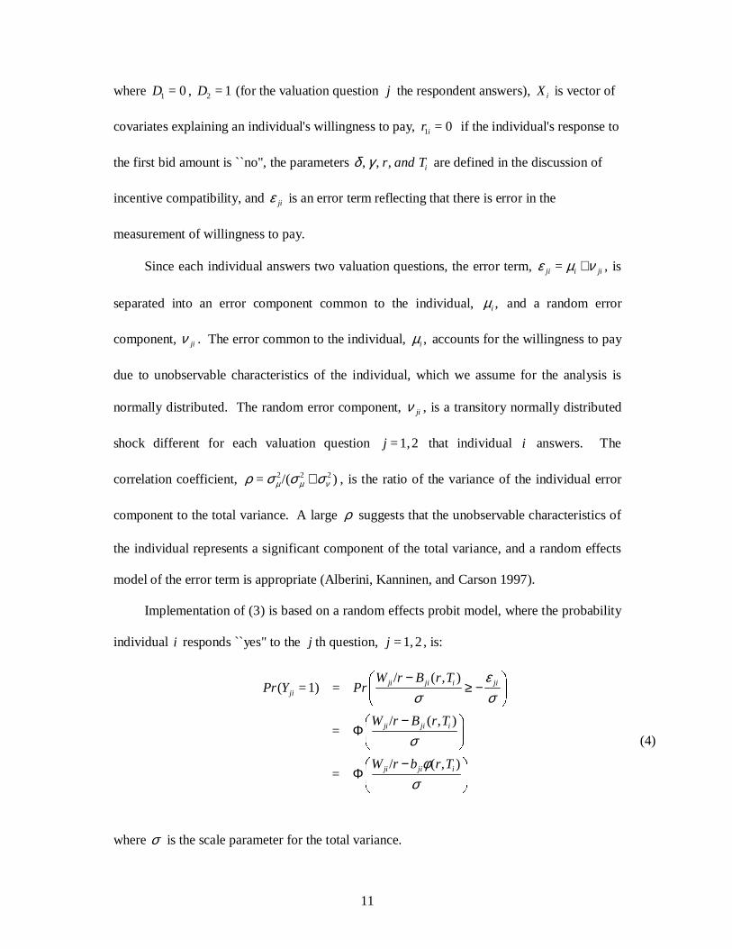
where 1 = 0D , 2 = 1D (for the valuation question j the respondent answers), iX is vector of
covariates explaining an individual's willingness to pay, 1 = 0ir if the individual's response to
the first bid amount is ``no", the parameters , , , ir and Tδ γ are defined in the discussion of
incentive compatibility, and jiε is an error term reflecting that there is error in the
measurement of willingness to pay.
Since each individual answers two valuation questions, the error term, =ji i jiε µ ν+ , is
separated into an error component common to the individual, ,iµ and a random error
component, jiν . The error common to the individual, ,iµ accounts for the willingness to pay
due to unobservable characteristics of the individual, which we assume for the analysis is
normally distributed. The random error component, jiν , is a transitory normally distributed
shock different for each valuation question =1,2j that individual i answers. The
correlation coefficient, 2 2 2= /( )µ µ νρ σ σ σ+ , is the ratio of the variance of the individual error
component to the total variance. A large ρ suggests that the unobservable characteristics of
the individual represents a significant component of the total variance, and a random effects
model of the error term is appropriate (Alberini, Kanninen, and Carson 1997).
Implementation of (3) is based on a random effects probit model, where the probability
individual i responds ``yes" to the j th question, =1,2j , is:
/ ( , )( =1) =
/ ( , )=
/ ( , )=
ji ji i jiji
ji ji i
ji ji i
W r B r TPr Y Pr
W r B r T
W r b r T
εσ σ
σφ
σ
−� �
≥ −� �� �
−� �
� �� �
−� �
� �� �
(4)
where σ is the scale parameter for the total variance.

12
Typically, by varying bid amounts across respondents, the scale parameter is directly
identified from the coefficient on the bid amount. However, since the bid amount is the net
present value of a finite stream of bids discounted by an unknown rate of time preference, r ,
the direct identification of either the scale parameter or the rate of time preference is not
possible since both are lumped together into the coefficient, ( , )ir Tφσ
− , on the per period bid
amount jib . Nonetheless, with additional variation in the length of the payment schedule, iT ,
across respondents, both the scale parameter and the rate of time preference can be identified.
To illustrate the identification method, suppose there is variation in the length of the
payment schedules, such that the payment schedules last for ˆ, ,T T� and T periods. In that
case, the coefficient on jib differs based upon the length of the payment schedule,
ˆ( , ) ( , ),
r T r Tφ φσ σ
− −�
and ( , )r Tφσ
− . The ratio of any two of the coefficients results in the
elimination of the scale parameter. For instance, for the payment schedules lasting ,T�
and T̂
periods, the ratio of the coefficients ( , )r Tφσ
−�
and ˆ( , )r Tφ
σ− is,
( , )ˆ( , )
r T
r T
φφ
�
. To use the
information contained in all the payment schedules, a ratio of coefficients is formed for a
payment schedule of each different length, and the ratios are summed together,
( , ) ( , )ˆ ˆ( , ) ( , )
r T r T
r T r T
φ φφ φ
+�
. The standard error of each ratio, or the sum of the ratios, is obtained from
the asymptotic covariance matrix by the Delta method (Greene 1997).
While the coefficients on the bid amounts come directly from the estimation of the
model (4), the determination of r from the ratio of the coefficients requires numerical
techniques separate from the original estimation. Indeed, since the ratio of coefficients is a
polynomial function of r , there are multiple solutions to the function, but nearly every
solution is imaginary with the exception of a single real root. The real solution to the

13
polynomial is the value used for r . The standard error of r is then obtained by simulation
methods using the Krinsky-Robb procedure (Haab and McConnell 2003).
The identification of the scale parameter, σ , along with the coefficients, β , γ , and δ
is readily obtained once the rate of time preference r is known. Median willingness to pay is
calculated from the estimates of the coefficients, β , at the mean of the independent variables,
X . The standard errors of the estimates of the parameters and the median willingness to pay
are obtained by the Delta method (Greene 1997).
IV. DATA
The data for this analysis come from a stated preference question within a mail survey
sent to single-family dwellings in Portland, Oregon to learn about the quality of and
recreation at regional parks in the city. Portland has a population of about half a million
people and is located in northern Oregon. The impressive natural features of the city include
two major rivers, the Willamette and Columbia, and roughly 10,000 acres of parks located in
places along ridges, plateaus, and volcanic peaks.
A random sample of 1,200 single-family dwellings selected from the 2001 Multnomah
County Assessor's data was mailed a packet containing an eight-page survey, a cover letter, a
map of the Portland-area highlighting seven regional parks, and a postage-paid return
envelope. The earliest versions of the survey were shown to individuals with knowledge and
expertise of Portland-area parks.i A focus group in Portland, three one-on-one sessions, and a
pre-test of the survey were done to ensure that the questions were carefully worded and
arranged. Of the 1141 deliverable surveys, 42% (479) were returned, and 88% (420) of those
surveys were useable in the analysis of the stated preference question.
Before reaching the stated preference question, which concerns the creation of
additional acreage for Powell Butte Park, a prominent regional park of Portland, the survey

14
asks questions about the quality and usage of the respondent's family of seven regional parks
in Portland, including Powell Butte. These questions and the map of the Portland-area help
the respondent to recall their experiences at Powell Butte. Although homes line the northern
side of Powell Butte, near the south-eastern boundary of the city, Portland's Parks and
Recreation Department is working to prevent additional development around the park. Also,
Portland has passed open space bond measures in the recent past, one in 1995, and another
one in November 2006 (Metro 2006).
The stated preference question initially describes the physical features and recreational
opportunities Powell Butte currently offers, and a detailed map of Powell Butte is available
for respondents to view. The proposal for additional park land at Powell Butte is as follows:
Several large parcels of land, totaling 100 acres, on the southeast side of Powell Butte
eventually will be purchased by developers, rezoned, and used to construct new
housing. Alternatively, the City could purchase these lands and create an addition to
Powell Butte Nature Park. Doing so would increase the size of the Park by 100 acres,
or 18%.
The payment vehicle described to the respondent is as follows:
One way to pay for these costs of enlarging Powell Butte Nature Park is to add
temporary surcharge (i.e., an additional payment) to the monthly water utility bills of
ALL businesses and households in Portland. The temporary surcharge would be in
effect for ______ months.
The respondents were randomly assigned a payment schedule and a set of three bids
values from four possible payment schedules, and, depending on the payment schedule, from
a list of five sets of bid values shown in Table 1.ii The payment schedules differ in the length
of time that the respondent makes payments for the public good, either 12 months, 48
months, 84 months, or 120 months. The first bid value in each set is the starting WTP bid for

15
the first question. If the respondent's answer to first question is `yes', the respondent is
offered the second bid value in the set, while a `no' response means that the third bid value is
offered.iii
At the bottom of the WTP question, respondents with a zero WTP were asked why their
WTP was zero. A respondent was presented with four options, ``I do not receive any benefits
from having a larger Powell Butte Park.'', ``I cannot afford to pay anything at this time.'', ``It
is unfair to ask people to pay more for parks.'', and ``Other (please list your reason)''. Several
respondents put a check next to the ``Other...'' option. Four wrote that water bills are too
high, and one wrote that they did not like the water bill payment mechanism. The protest bids
identified from this question about zero WTP were removed before conducting the analysis.
Hypothetical bias may affect the results, even though respondents are likely familiar
and comfortable with open space issues in Portland. There is unfortunately no way to know
in what direction the bias might exist unless there are unknown queues in the proposal for
additional park land at Powell Butte. Hypothetical bias is unlikely to affect the estimates of
the discount rate (unless the proposal somehow indicates the additional park land has less
value in the future) since the discounts rates are estimated through the payment schedules,
and the payment schedules have minimal description that might send unknown queues to the
respondent.
The survey collects information in addition to the socioeconomic characteristics of the
respondent useful for understanding the respondent's WTP for additional park land at Powell
Butte. The extra information includes whether the respondent commutes, the number of
hours the respondent works for pay in a week, whether the respondent intends to remain at
that residence for the rest of their life, and the number of trips and average on-site time spent
at Powell Butte. Travel times and distances to Powell Butte from each respondent's residence
were determined using network analyst in GIS.iv The respondent's perception of the hiking

16
quality and cleanliness of the grounds at Powell Butte were obtained from nine-scale Likert-
type questions.
Descriptive statistics of the sample and population are shown in Table 2. The sample
has on average higher incomes and less family members, is more educated, and is more
representative of females than the population. The sample is evenly spread across the four
payment schedules since roughly a quarter of the sample responds to each payment schedule.
The large variation in the hours spent working for pay by the respondent is because many of
the respondents are homemakers.
V. EMPIRICAL RESULTS
We report the results from six models of willingness to pay responses. All models are
estimated by random effects probit regressions except for the single bounded model that is
estimated by a regular probit. The naive double-bounded models (Double and Shift) do not
control for anchoring, and framing effects, while the most sophisticated double-bounded
model (Fram, Anch & Shift) controls for all the effects.
In the estimation of the models, we pool the data from all the payment schedules. The
coefficient on the bid amount should differ based upon the payment schedule that the
respondent is answering since the annuity factor, ( , )ir Tφ , embedded in the coefficient, differs
across payment schedules. Dummy variables for the 48, 84, and 120 month payment
schedules interacted with the bid amount for those payment schedules allows the coefficient
on the bid amount to differ across the payment schedules.
Table 3 has the coefficients on the bid amounts for each of the payment schedule
lengths for the WTP models. Except for the single-bounded model, the coefficient on the 12
month bid amount is negative and significant at the 5% level. The insignificant coefficient on
the 12 month bid amount for the single-bounded model makes us dubious of the value for the

17
discount rate we find for that model. In all the models, the coefficient on the bid amount for
the 84 month payment schedules is more negative than the coefficient on the 12 month bid
amount, with significance at the 5% level.
For the naive double-bounded models, there is no significant difference between the bid
amount coefficients on the 12 and 48 month payment schedules, but there is a significant
difference between the bid amount coefficients on 48 and 84 month payment schedules at the
10% level. For the more sophisticated double-bounded models, there is a significant
difference between the bid amount coefficients on 12 and 48 month payment schedules at the
10% level, but there is no significant difference between the bid amount coefficients on the
48 and 84 month payment schedules (except for the model, Anchoring & Shift). In all the
models, there is no significant difference between the bid amount coefficients on 84 and 120
month payment schedules, suggesting respondents do not distinguish between the seven and
ten year payment schedules when considering whether to support the proposal.
The component of the error term attributable to individual effects, ρ , ranges from 0.52
to 0.73, where the lower values of ρ are found in the naive double-bounded models and the
higher values of ρ are found in the models controlling for framing effects. Although
individual effects have a larger role in the models controlling for violations of incentive
compatibility, their presence is certain in all the double-bounded models.
Table 4 has the findings of the annualized rate of time preference (discount rate) for the
models of willingness to pay response. The annualized discount rate is found using only the
12 and 48 month payment schedules, the 12 and 84 month payment schedules, the 12 and 120
month payment schedules, and all of the payment schedules. Other than the findings of the
single-bounded model, the discount rate is the largest when only the 12 and 48 month
payment schedules are used.
An explanation for the higher discount rates when only the 12 and 48 month payment

18
schedules are used comes from the studies utilizing experiments to find discount rates. Thaler
(1981) and Benizon et al. (1989) find in experiments of tradeoffs between a payoff now
versus later that extending the wait time for a payoff later results in a lower discount rate for
participants. They also find that larger payoffs result in lower discount rates for the
participants. We speculate that for the 84 and 120 month payment schedules, where a
substantial proportion of the payments occur far off in the future, the respondents make their
choices with a lower discount in mind in line with the findings of the experimental studies.
The somewhat lower discount rate for the 84 versus 120 month payment schedules we
attribute to the larger payments respondents see for the 84 month payment schedule.
In all the models, the discount rate found using only the 12 and 84 month payment
schedules or only the 12 and 120 month payment schedules is close to the discount rate found
using all the payment schedules. The discount rate for the single-bounded model is low at
0.144, but this finding is questionable since the coefficient on the 12 month bid amount is not
significant for the single-bounded model. The discount rate for the naive double-bounded
models is around 0.30 while the discount rate for the more sophisticated models is around
0.35. The distributions around the discount rates are corrected by trimming off the highest
2.5% of values since there is significant skewness in the upper tail. The standard errors of
around 0.25 shown in Table 4 come from the distributions corrected for skewness.
With the discount rates found using all the payment schedules, estimates of the monthly
WTP, scale, and follow-up question modifiers are shown in Table 5. The log-likelihood
statistic is the criterion for the comparison of the WTP models. Unlike the shift parameter,
the anchoring parameter improves the fit of the model significantly over the naive double-
bounded model. Assuming that the anchoring effect only occurs in the ascending sequence
of the follow-up questions further improves the fit of the model suggesting that only the
ascending sequence of follow-up questions is not incentive incompatibile.

19
The monthly WTP ranges from near 3 for single-bounded and the naive double-
bounded models to 4.5 for the models controlling for anchoring and framing effects. The
more sophisticated double-bounded models have lower standard errors for monthly WTP
although, in general, the standard errors across different random effects probit regressions are
not possible to predict (Collett 1991).
The model with only a shift effect (Shift) finds that the shift parameter is nearly
significant, but the models with both anchoring and shift effects (Anchoring & Shift, and
Fram, Anch & Shift ) find an insignificant shift parameter. The nearly significant shift
parameter found in the model with only a shift effect is an artifact of the misspecification
resulting from the exclusion of the anchoring parameter.
For all the models with an anchoring effect, the anchoring parameter is significant
although small. The anchoring parameter is small since the representation of the anchoring in
the WTP model is not on the monthly bid amount shown in the CVM question, which would
make the anchoring parameter larger, but on the full bid amount. Comparing the WTP
models, the anchoring parameter is larger if the WTP model only allows for the anchoring
effect in the ascending sequence of the follow-up questions. The argument by DeShazo
(2002) that violations of incentive compatibility are only present in the ascending sequence of
follow-up questions is consistent with that finding. A WTP model, not shown in the tables,
where the anchoring effect is only present in the descending sequence of the follow-up
questions results in an anchoring parameter that is insignificant.
Tables 6 shows estimates of the coefficient vector β , the scale σ , the anchoring and
shift parameters, γ and δ , for four WTP models. Aside from the single-bounded model
shown for comparison, the three other WTP models chosen from the six models shown in
Tables 3 to 6 are the models thought to best represent the WTP responses. If the anchoring
effect occurs in both the descending and ascending sequences of the follow-up questions,

20
then Anchoring & Shift is the appropriate model of the WTP responses. However,
comparison of the WTP models by the log-likelihood criterion suggests that anchoring, for
the most part, is only present in the ascending sequence of the WTP responses. The model
Framing is appropriate if the anchoring effect is significant enough that the ascending
sequence of WTP responses offers no new information. However, if the anchoring effect is
weak, the model Fram, Anch & Shift keeps the information in the ascending sequence of
WTP responses. The standard errors of coefficient estimates are the lowest for the models
Framing and Fram, Anch & Shift.
As expected, the more education (EDU) and income (INC) a respondent has the more
their WTP for additional public open space. Also, we find that the more hours worked in a
week (WRKHRS) and the larger the size of the family (FAMSIZE) of the respondent the
lower their WTP. Since the additional open space is adjacent to Powell Butte, a large
wilderness park, the major beneficiaries of the additional open space are the main users of
Powell Butte, outdoor enthusiasts. Outdoor enthusiasts are typically educated professionals
without children whose main constraint on recreation is their amount of leisure time.
Since outdoor enthusiasts usually spend a lot of time on-site at wilderness parks
exploring the hiking trails, we find that on-site time (SITETIME) and the perception of the
quality of the hiking trails (HIKING) increases WTP. The sign of the coefficient for the
distance of the respondent's residence from Powell Butte (TRVLDIST) is the wrong sign but
not significant, and the sign of the coefficient for the travel time to Powell Butte
(TRVLTIME) is the expected sign but also not significant. Since all the respondents live in
the Portland-area, there may be inadequate variation in TRVLDIST and TRVLTIME to
obtain significant coefficients for those variables.
The respondent's WTP is not sensitive to the length of the payment schedule since none
of the coefficients for the length of the payment schedule (PAYSCHY4, PAYSCHY7,

21
PAYSCHY10) are significant. However, since the coefficients for the length of the payment
schedule are strongly correlated to the coefficient on the bid amount, the omission of the
binary variables for the length of the payment schedule would result in bias of all the
parameter estimates.
Table 7 shows the sensitivity of the monthly WTP and the full WTP for additional park
land at Powell Butte to the choice of discount rate. The choice of the lower bound of the
discount rate results in a lower monthly WTP but a higher full WTP, and the choice of the
upper bound of the discount rate results in a higher monthly WTP but a lower full WTP. The
interval of the discount rate is wide enough that the 95% confidence intervals of either the
monthly or full WTPs rarely overlap. Comparing the WTP models, since the discount rate
intervals are similar across models, the monthly and full WTP intervals are also similar. The
full WTP is the most sensitive to the choice of discount rate since the full WTP is the net
present value of a stream of monthly WTPs. If the median discount rate is chosen, the full
WTP for an additional 100 acres of open space adjacent to Powell Butte is about $165 per
household.
With information already available on discount rates, a CVM question could ask the
WTP for a month of benefits rather than the WTP for a long time horizon of benefits, since
the former question is much less mentally cumbersome. Combining information on the WTP
for a month of benefits and the discount rate easily allows for a determination of the WTP for
a long time horizon, assuming the monthly WTP does not change over time.
If the individual discount rate for public goods is much higher than the rates currently
used in public investment decision making, the economic feasibility of a public investment is
much more dependent on the ability to front-load the benefits of the public good rather than
having most of the benefits received far off into the future.
Table 8 shows the influence of demographic characteristics on the implicit discount

22
rate. We stratify the sample by a demographic characteristic and see what the discount rate
for each stratified segment is. The demographic characteristics examined are age, education,
participation in an environmental organization, income, average number of work hours per
week, and the presence of children 14 or younger living in the same household as the
respondent.v Since Fram, Anch & Shift is the WTP model with the best fit, we use that
model for determining the implicit discount rate of the stratified samples. The number of
observations in each of the stratified samples is shown in the last column of Table 8.
A comparison of the discount rates across the stratified samples for each of the
demographic characteristics reveals that most of the demographic characteristics do not
statistically influence the discount rate. The 90% confidence intervals for discount rates
stratified by a given demographic characteristic (in particular, education, participation in an
environmental organization, income, and average number of work hours per week) overlap
significantly suggesting that the discount rates are not statistically different from each other.
However, the age of the respondent and the presence of young children living in the
same household as the respondent do appear to statistically influence the discount rate.
Younger respondents have a lower discount rate than older respondents, and respondents with
no children have a much lower discount rate than respondents with children. Selfish
concerns unique to those demographics are a possible explanation for the findings.vi
Since older people are less likely to benefit from additional open space in the future
than younger people, due to the frailty of old age and the higher chance mortality, older
people would be expected to higher discount rates. Parents with young children want their
children to enjoy the benefits of open space before their children turn into adults. Since
parents of young children benefit less from open space in the distant future than people
without children, parents with young children would be expected to have higher discount
rates than people without children.

23
If the discount rate for public goods is dependent on demographics, public investment
decision makers should pay attention to the demographics of the area where a public good is
being created while considering how the benefits of the public good will be provided over
time.
VI. CONCLUSION
Our CVM study finds both individual discount rates and the WTP for additional open
space. Discount rates are found through variation across surveys in the length of the payment
schedule for the public good, additional public open space; four different time frames are
used. Discount rates are higher if the shorter time frame payment schedules are used.
Discount rates show some sensitivity to the model of WTP responses, where the more
sophisticated double-bounded models take into account shift, anchoring, and framing effects.
If all the payment schedules are used for the more sophisticated models of WTP responses,
discount rates of around 0.30 are found, similar to the rates found in revealed preference and
experimental studies, and lower than the rates found in the prior CVM studies.
The WTP component of the CVM question is for additional public open space adjacent
to a prominent regional park in Portland, Oregon. We find the median WTP is $165 per
household for an additional 100 acres of park land, much lower than $234 for a 5.5 acre
parcel in Boulder (Breffle, Morey, and Loder 1998). We speculate that the lower WTP in our
study is because the additional land is adjacent to an already large regional park. The
significant explanatory factors of WTP are education, income, hours worked per week,
family size, amount of time spent at regional parks in Portland, and the perception of the
hiking trails at Powell Butte. Respondents that are educated outdoor enthusiasts are the
strongest supporters of open space preservation.
The full WTP for a public good is shown to be sensitive to the assumption of the

24
discount rate. Additional research might investigate whether the stream of benefits is stable
over time and whether every future benefit goes into the mental calculation that produces the
full WTP. The discounts rates are stratified by demographics, and the discount rate is shown
to be sensitive to age of the respondent and presence of young children living in the same
household as the respondent. Additional research might investigate whether other public
goods are sensitive to the same demographics or whether this finding is unique to public open
space. Also, research might look at how riskiness (perceived or actual) related to the
provision of the public good influences the discount rate.
Public investment decision makers need to consider how the benefits of a public good
are provided over time, in particular how to front-load more of the benefits in light of the
finding that individual discount rates are higher than market rates. Also, policy makers should
know the demographics of the area where the public good is created while considering how
the benefits of the public good will be provided over time.

25
References
Alberini, Anna, Barbara Kanninen, Richard Carson. 1997. ``Modeling Response Incentive
Effects in Dichotomous Choice Contingent Valuation Data.'', Land Economics 73 (3):
309-324.
Ausubel, Lawerence. 1991. ``The Failure of Competition in the Credit Card Market'',
American Economic Review 81 (1): 50-81.
Benzion, Uri, Amnon Rapoport, Joseph Yagil. 1989. ``Discount Rates Inferred from
Decisions: An Experimental Study.'', Management Science 35: 270-84.
Breffle, William, Edward Morey, Tymon Lodder. 1998. ``Using Contingent Valuation to
Estimate a Neighborhood's Willingness to Pay to Preserve Undeveloped Urban Land.'',
Urban Studies 35 (4): 715-27.
Collett, D.. 1991. Modelling Binary Data. London: Chapman and Hall.
Crocker, T.D., J. F. Shogen. 1993. ``Dynamic Inconsistency in Valuing Environmental
Goods.'', Ecological Economics 7: 239-54.
Cropper, Maureen, Sema Ayede, Paul Portney. 1994. ``Preference for Life Saving Programs:
How the Public Discounts Time and Age.'', Journal of Risk and Uncertainty 8: 243-265.
DeShazo, J.R.. 2002. ``Designing Transactions without Framing Effects in Question
Formats.'', Journal of Environmental Economics and Management 43: 360-385.
Flachaire, Emmanuel, Guillaume Hollard. 2006. ``Controlling Starting-Point Bias in Double-
Bounded Contingent Valuation Surveys.'', Land Economics 82 (1): 103-111.
Gately, Dermot. 1980. ``Individual Discount Rate and the Purchase and Utilization of
Energy-Using Durables: Comment.'', Bell Journal of Economics 11: 373-374.
Greene, William. 1997. Econometric Analysis, 3rd Edition. New York: Prentice Hall.
Haab, T.C., K.E. McConnell. 2003. Valuing Environmental and Natural Resources. Edwar
Elgar.

26
Harrison, Glenn, Morten Lau, Melonie Williams. 2002. ``Estimating Individual Discount
Rates in Denmark: A Field Experiment.'', American Economic Review 92 (5): 1606-
1617.
Hausman, Jerry. 1979. ``Individual Discount Rate and the Purchase and Utilization of
Energy-Using Durables.'', Bell Journal of Economics 10: 172-183.
Herriges, Joseph, Jason F. Shogren. 1996. ``Starting Point Bias in Dichotomous Choice
Valuation with Follow-Up Questioning.'', Journal of Environmental Economics and
Management 30: 112-131.
Lindsey, Gret, G. Knapp. 1999. ``Willingness to Pay for Urban Greenway Projects.'' Journal
of American Planning Association 65 (3): 297-313.
McConnell, Virginia, Margaret Walls. 2005. The Value of Open Space: Evidence from
Studies of Nonmarket Benefits. Resources for the Future.
Metro. 2006. “1995 open spaces bond measures.”
http://www.metro-region.org/article.cfm?articleID=144 (March 21, 2007).
Ruderman, Henry, Mark Levine, James McMahon. 1986. ``Energy-Efficiency Choice in the
Purchase of Residential Appliances.'', In Kempton, Willett, and Max Neiman, eds.,
Energy Efficiency: Perspectives on Individual Behavior. Washington D.C.: American
Council for an Energy Efficient Economy.
Stevens, Thomas, Nichole DeCoteau, Cleve Willis. 1997. ``Sensitivity of Contingent
Valuation to Alternative Payment Schedules.'', Land Economics 73 (1): 140-48.
Thaler, Richard. 1981. ``Some Empirical Evidence on Dynamic Inconsistency'', Economic
Letters 8: 201-207.
Tyrva� �
inen, Liisa, Hannu Vaananen. 1998. ``The Economic Value of Urban Forest
Amenities: An Application of the Contingent Valuation Method.'', Landscape and
Urban Planning 43: 105-18.

27
Warner, John T., Saul Pleeter. 2001. ``The Personal Discount Rate: Evidence from Military
Downsizing Programs.'', American Economic Review 91 (1): 33-53.
Whitehead, John. 2002. ''Incentive Incompatibility and Starting-Point Bias in Iterative
Valuation Questions.'', Land Economics 78 (2): 285-97.
Whitehead, John. 2004. ''Incentive Incompatibility and Starting-Point Bias in Iterative
Valuation Questions: Reply.'', Land Economics 80 (2): 316-319.
28
Endnotes i We thank Noelwah Netusil of Reed College, staff of the Metro's Regional Parks and Greenspaces Department,
and staff of the Portland Parks and Recreation Department.
ii The bids used in each payment schedule were designed so that the present value of payments is the same
across all treatments. They are based in each case on the present results for mean and standard error of monthly
willingness to pay, adjusted by the difference in the annuity factors between each treatment and the pretest. Thus
the bids for shorter treatments are higher than those for longer treatments.
iii The use of a follow-up WTP question is somewhat unusual for mail surveys, as it is more commonly used in
telephone or in-person surveys. It is more accurately termed a random payment card approach, where the
random variation in the category bounds helps mitigate concerns about framing effects that normally are
expressed about payment card formats. (The explicit modeling of framing effects helps address this too.)
Because the respondent can potentially see all three bids at once, it is analogous to asking a slightly more
involved single bound WTP question. As the incentive compatibility properties of this format have not been
studied carefully yet, some caution is needed in interpreting WTP estimates derived from it.
iv We thank Shawn Bucholtz of the Economic Research Service of the USDA for help with this data.
v The gender of the respondent was also considered, but the relatively low number of males that responded
prevented estimation of the male segment of the sample.
vi Cropper et al. (1994) reach similar conclusions in their analysis of preferences for life saving programs.

29
TABLE 1
Payment schedules and bid value sets for additional open space in the CVM questionnaire
Bid value sets Additional Open Space Observations yy yn ny nn yy% yn% ny% nn% One year payment schedule Set 1 (12,27,6) 19 2 6 3 8 10.5 31.6 15.8 42.1 Set 2 (21,36,12) 17 2 2 4 9 11.8 11.8 23.5 52.9 Set 3 (30,45,21) 21 3 2 6 10 14.3 9.5 28.6 47.6 Set 4 (39,54,30) 23 1 6 3 13 4.3 26.1 13.0 56.5 Set 5 (48,63,39) 12 2 0 1 9 16.7 0.0 8.3 75.0 Four year payment schedule Set 1 (6,14,3) 30 5 11 5 9 16.7 36.7 16.7 30.0 Set 2 (11,18,6) 17 3 1 6 7 17.6 5.9 35.3 41.2 Set 3 (15,23,11) 20 2 4 4 10 10.0 20.0 20.0 50.0 Set 4 (20,27,15) 17 2 1 3 11 11.8 5.9 17.6 64.7 Set 5 (24,32,20) 24 4 2 1 17 16.7 8.3 4.2 70.8 Seven year payment schedule Set 1 (5,11,2) 22 4 9 3 6 18.2 40.9 13.6 27.3 Set 2 (8,14,5) 27 5 8 3 11 18.5 29.6 11.1 40.7 Set 3 (12,18,8) 26 1 6 5 14 3.8 23.1 19.2 53.8 Set 4 (16,22,12) 22 3 1 4 14 13.6 4.5 18.2 63.6 Set 5 (19,25,16) 17 1 1 1 14 5.9 5.9 5.9 82.4 Ten year payment schedule Set 1 (4,10,2) 22 2 10 4 6 9.1 45.5 18.2 27.3 Set 2 (8,13,4) 32 6 8 4 14 18.8 25.0 12.5 43.8 Set 3 (11,17,8) 6 2 1 0 3 33.3 16.7 0.0 50.0 Set 4 (14,20,11) 18 1 2 4 11 5.6 11.1 22.2 61.1 Set 5 (18,23,14) 28 2 5 1 20 7.1 17.9 3.6 71.4

30
TABLE 2
Definitions and summary statistics of variables
Variables Definition Sample Mean
Sample Std. Dev.
2004 Population Meana
SEX =1 if the respondent is male 0.35 -- 0.49 AGE Age 40.43 10.27 37.2 EDU Years of schooling 16.81 2.45 14.26
ENV =1 if respondent has ever belonged to an environmental organization 0.61 -- --
INC Annual family income 76184 44169 68305
WRKHRS Hours respondent spends working for pay per week
32.62 17.29 --
COMMUTE =1 if respondent commutes to work at least one day a week
0.78 -- --
FAMSIZE Size of family living in the same household as the respondent
2.55 1.27 3.14
CHILD Number of children in the family age fourteen or younger living in the same household as the respondent
0.61 0.93 0.42
RESTIME =1 if the respondent expects to stay in their current residence for the rest of their life
0.23 -- --
TRVLDIST Distance to Powell Butte using major roadways (miles)
8.19 3.75 --
TRVLTIME Travel time to Powell Butte using major roadways (minutes) 11.53 4.44 --
SITETIME The sum of the average on-site time spent per trip at five regional parks in the Portland-areab
200.59 158.74 --
HIKING An index from 0 to 9 that measures the respondent's perception of the quality of Powell Butte's hiking trails
6.9 1.18 --
CLEAN An index from 0 to 9 that measures the respondent's perception of the cleanliness of the grounds at Powell Butte
8.05 1.65 --
PAYSCHY4 =1 if respondent bids with a payment schedule lasting 48 months
0.26 -- --
PAYSCHY7 =1 if respondent bids with a payment schedule lasting 84 months
0.27 -- --
PAYSCHY10 =1 if respondent bids with a payment schedule lasting 120 months 0.25 -- --
a The total population of the Portland, Oregon is 524,944. The summary statistics of the population come
from the U.S. Census Bureau, 2004 American Community Survey.
b The five regional parks are Forest Park, Mount Tabor Park, Tryon Creek State Park, Willamette Park,
and Powell Butte Park.

31
TABLE 3
Bid coefficient estimates for models of WTP
Bid Coefficients Model One Year Four Years Seven Years Ten Years
Single -0.015 (0.013)
-0.045 (0.019)**
-0.105 (0.029)***
-0.078 (0.026)***
Double -0.028
(0.015)** -0.059
(0.026)** -0.118
(0.039)*** -0.110
(0.037)***
Shift -0.028
(0.014)** -0.056
(0.025)** -0.114
(0.038)*** -0.106
(0.035)***
Anchoring & Shift -0.045 (0.021)**
-0.092 (0.037)**
-0.163 (0.053)***
-0.141 (0.049)***
Framing -0.049
(0.024)** -0.117
(0.045)*** -0.175
(0.062)*** -0.147
(0.056)***
Fram, Anch & Shift -0.050 (0.026)**
-0.230 (0.048)***
-0.179 (0.066)***
-0.148 (0.057)***
Note: All models other than Single are estimated with random effects. Standard errors in parentheses. *,**,***
indicate significance at the 10%, 5%, and 1% levels.

32
TABLE 4
Annual implicit discount rates determined from the bid coefficient estimates
Payment Schedules
Model One & Four Years One & Seven Years
One & Ten Years All Years
Single 0.069 (0.466)
-0.045 (0.209)
0.142 (0.274)
0.144 (0.266)
Double 0.504
(0.513)** 0.196
(0.241)* 0.284
(0.214)*** 0.294
(0.277)***
Shift 0.503 (0.501)**
0.633 (0.519)*
0.301 (0.273)***
0.303 (0.306)***
Anchoring & Shift 0.519 (0.501)**
0.267 (0.228)***
0.375 (0.298)***
0.369 (0.247)***
Framing 0.714
(0.286)* 0.268
(0.278)*** 0.389
(0.355)*** 0.337
(0.318)***
Fram, Anch & Shift 0.389 (0.485)*
0.255 (0.262)**
0.397 (0.319)***
0.354 (0.300)***
Note: All models other than Single are estimated with random effects. Standard errors in parentheses. *,**,***
indicate significance at the 10%, 5%, and 1% levels.

33
TABLE 5
Mean, scale, and follow-up question modifiers of monthly WTPs
Model µ σ γ δ r LL
Single 2.70 (0.95)***
719.72 (199.68)
-- -- 0.144 (0.266)
- 235.72
Double 2.59
(1.56)*** 371.96
(117.97)*** -- -- 0.294
(0.277)*** - 478.81
Shift 3.17
(1.37)** 381.86
(118.58)*** -- -1.44 (1.15)
0.303 (0.306)*** - 477.9
Anchoring & Shift 4.63 (1.19)***
225.29 (71.87)**
0.012 (0.005)**
2.22 (10.92)
0.367 (0.25)***
- 468.1
Framing 4.66
(1.07)*** 211.19
(68.53)*** -- -- 0.337
(0.318)*** - 382.9
Fram, Anch & Shift 4.79 (1.06)***
201.42 (66.61)***
0.039 (0.012)***
3.13 (15.88)
0.354 (0.300)***
- 458.7
Note: All models other than Single are estimated with random effects. Standard errors in parentheses.
*,**,*** indicate significance at the 10%, 5%, and 1% levels.

34
TABLE 6
Parameter estimates for the explanatory factors of WTP for additional public open
space
Variables Single Anchoring &Shift Framing Fram, Anch, & Shift
CONSTANT -6.159 (8.209)
-6.808 (10.279)
-6.564 (8.871)
-6.571 (8.700)
SEX 1.757
(1.386) 2.617
(1.835) 1.642
(1.536) 2.256
(1.657)
AGE -0.083 (0.069)
-0.104 (0.092)
-0.113 (0.078)
-0.111 (0.076)
EDU 0.339 (0.263)
0.528 (0.349)
0.506 (0.299)*
0.519 (0.293)*
ENV 1.162
(1.294) 1.747
(1.731) 2.034
(1.478) 2.178
(1.463)
INC 3.81E-5
(1.76E-5)** 5.15E-5
(2.21E-5)** 4.00E-5
(1.80E-5)** 3.92E-5
(1.78E-5)**
WRKHRS -0.071 (0.039)*
-0.106 (0.053)**
-0.074 (0.044)*
-0.079 (0.044)*
COMMUTE -1.281 (1.561)
-1.231 (2.079)
-2.229 (1.826)
-2.283 (1.822)
FAMSIZE -0.994
(0.577)* -1.348
(0.749)* -1.131
(0.606)* -1.159
(0.599)*
CHILD -0.347 (0.670)
-0.573 (0.925)
-0.329 (0.773)
-0.365 (0.772)
RESTIME -2.373 (1.736)
-3.029 (2.248)
-1.307 (1.782)
-1.161 (1.757)
TRVLDIST 0.996 (0.932)
1.512 (1.257)
1.377 (1.059)
1.438 (1.048)
TRVLTIME -0.750 (0.779)
-1.129 (1.053)
-1.036 (0.888)
-1.091 (0.876)
SITETIME 0.005
(0.004) 0.008
(0.005) 0.008
(0.005)* 0.008
(0.005)*
HIKING 1.073 (0.614)*
1.521 (0.797)*
1.415 (0.666)**
1.395 (0.652)**
CLEAN -0.430 (0.395)
-0.577 (0.529)
-0.391 (0.454)
-0.362 (0.446)
PAYSCHY4 2.974
(4.495) 1.665
(4.259) 2.637
(4.138) 2.699
(4.076)
PAYSCHY7 8.105
(5.751) 5.830
(4.761) 4.171
(4.442) 4.158
(4.386)
PAYSCHY10 5.556 (5.001)
4.209 (4.518)
2.015 (4.215)
1.849 (4.138)
σ 719.724 (199.676)***
225.285 (71.871)***
211.192 (65.528)***
201.421 (66.609)***
γ -- 0.012
(0.005)** -- 0.039
(0.012)***
δ -- 2.222
(10.917) --
3.125 (15.867)
r 0.144
(0.266) 0.369
(0.247)*** 0.337
(0.318)*** 0.354
(0.300)*** Note: All models other than Single are estimated with random effects. Standard errors in parentheses.
*,**,*** indicate significance at the 10%, 5%, and 1% levels.

35
TABLE 7
Sensitivity of the monthly WTP, µ , and the WTP, r/12
µ, to the assumption of the discount
rate
Discount rate interval Model 2.5% Lower Bound Median 2.5% Upper Bound Anchoring & Shift r 0.146 0.369 1.063
µ 2.876 (0.752)***
4.629 (1.192)***
6.413 (1.653)***
r/12
µ
235.69 (61.61)***
150.80 (38.82)***
72.06 (18.57)***
Framing r 0.100 0.337 1.303
µ 2.341 (0.554)***
4.655 (1.072)***
6.976 (1.649)***
r/12
µ
280.42 (66.39)***
166.27 (38.27)***
64.24 (15.19)***
Fram, Anch & Shift r 0.115 0.354 1.305
µ 2.641 (0.601)***
4.799 (1.058)***
7.121 (1.612)***
r/12
µ
276.37 (62.83)***
165.51 (36.52)***
65.51 (14.83)***
Note: Standard errors in parentheses. *,**,*** indicate significance at the 10%, 5%, and 1% levels.

36
TABLE 8
Implicit annual discount rates stratified by demographics
Demographic characteristic Discount Rate
Standard Error
90% Confidence Interval Observations
All 0.354 0.300 0.167 0.832 840 Younger than forty 0.078 0.264 -0.074 0.501 478 Forty or older 0.790 0.564 0.447 1.761 362 College education 0.187 0.356 -0.011 0.705 454 Education beyond college 0.304 0.377 0.103 0.931 386 Do not belong to enviro-organization 0.315 0.389 0.082 0.992 324 Belong to enviro-organization 0.435 0.349 0.207 1.023 516 Lower middle income 0.085 0.243 -0.081 0.482 378 Upper middle income 0.483 0.462 0.224 1.297 372 Work less than 40 hrs per week 0.299 0.155 0.177 0.562 326 Work more than 40 hrs per week 0.302 0.148 0.186 0.547 514 No children -0.235 0.189 -0.367 0.061 520 Have children 1.032 0.654 0.592 2.127 320 Note: Fram, Anch & Shift model is used to identify implicit discount rates.