Identifying consumer-resource population dynamics usingpaleoecological data

Einarsson, Á., Hauptfleisch, U., Leavitt, P. R., & Ives, A. R. (2016). Identifying consumer-resource populationdynamics using paleoecological data. Ecology, 97(2), 361-371. https://doi.org/10.1890/15-0596.1

Published in:Ecology

Document Version:Peer reviewed version

Queen's University Belfast - Research Portal:Link to publication record in Queen's University Belfast Research Portal

Publisher rightsCopyright 2016 Ecological Society of America. This work is made available online in accordance with the publisher’s policies. Please refer toany applicable terms of use of the publisher.

General rightsCopyright for the publications made accessible via the Queen's University Belfast Research Portal is retained by the author(s) and / or othercopyright owners and it is a condition of accessing these publications that users recognise and abide by the legal requirements associatedwith these rights.

Take down policyThe Research Portal is Queen's institutional repository that provides access to Queen's research output. Every effort has been made toensure that content in the Research Portal does not infringe any person's rights, or applicable UK laws. If you discover content in theResearch Portal that you believe breaches copyright or violates any law, please contact openaccess@qub.ac.uk.

Download date:17. Mar. 2022

1

Identifying consumer-resource population dynamics using paleoecological data 1

2

3

Árni Einarsson1,2, Ulf Hauptfleisch1, 3, Peter R. Leavitt4, Anthony R. Ives5 4

5

1 Mývatn Research Station, IS-660 Mývatn, Iceland 6

7

2 Institute of Life- and Environmental Sciences, Askja, Sturlugata 7, University of Iceland, IS-101 8

Reykjavík, Iceland 9

10

3 Faculty of Earth Sciences, Askja, Sturlugata 7, University of Iceland, IS-101 Reykjavík, Iceland 11

12

4 Department of Biology, University of Regina, Regina, SK, Canada S4S 0A2 13

14

5 Department of Zoology, University of Wisconsin, Madison, WI 53706, USA 15

16

17

18

2

ABSTRACT 19

Ecologists have long been fascinated by cyclic population fluctuations, because they suggest 20

strong interactions between exploiter and victim species. Nonetheless, even for populations 21

showing high-amplitude fluctuations, it is often hard to identify which species are the key drivers 22

of the dynamics, because data are generally only available for a single species. Here, we use a 23

paleoecological approach to investigate fluctuations in the midge population in Lake Mývatn, 24

Iceland, which ranges over several orders of magnitude in irregular, multi-generation cycles. 25

Previous circumstantial evidence points to consumer-resource interactions between midges and 26

their primary food, diatoms, as the cause of these high-amplitude fluctuations. Using a pair of 27

sediment cores from the lake, we reconstructed 26 years of dynamics of midges using egg 28

remains, and algal groups using diagnostic pigments. We analyzed these data using statistical 29

methods that account for both the autocorrelated nature of paleoecological data and measurement 30

error caused by the mixing of sediment layers. The analyses revealed a signature of consumer-31

resource interactions in the fluctuations of midges and diatoms: diatom abundance (as inferred 32

from biomarker pigment diatoxanthin) increased when midge abundance was low, and midge 33

abundance (inferred from egg capsules) decreased when diatom abundance was low. Similar 34

patterns were not found for pigments characterizing the other dominant algal group in the lake 35

(cyanobacteria), subdominant algae (cryptophytes), or ubiquitous but chemically unstable 36

biomarkers of total algal abundance (chlorophyll-a); however, a significant but weaker pattern 37

was found for the chemically stable indicator of total algal populations (-carotene) to which 38

diatoms are the dominant contributor. These analyses provide the first paleoecological evaluation 39

of specific trophic interactions underlying high amplitude population fluctuations in lakes. 40

41

3

Key words: fossil pigments; Lake Mývatn; Chironomidae; diatoms; population fluctuations; 42

consumer-resource dynamics; Iceland. 43

44

4

INTRODUCTION 45

Cyclic population dynamics have generated one of the oldest and largest bodies of 46

literature in ecology, starting with the classic models of Lotka showing that population cycles can 47

be generated by predator-prey, or more generally, exploiter-victim interactions (Lotka 1925). 48

Population cycles have generated this interest because they are an easily observed signal of 49

strong interactions among species (Kendall et al. 1999). Despite the numerous population cycles 50

that have been documented, in many cases it is unclear what are the key species driving the 51

cycles. For the iconic snowshoe hare cycles, only extensive research over many decades led to 52

the generally accepted hypothesis that cycles are driven primarily by predation from lynx and 53

other specialist predators, with secondary importance attributed to interactions with the hare food 54

base (Krebs et al. 1995, Krebs 2011). At high latitudes, cycles of microtine rodent populations 55

are common, yet there is still debate over the relative importance of top-down interactions 56

between rodents and predators in driving the cycles (Stenseth 1999, Turchin and Hanski 2001). 57

For insects, numerous cyclic populations have been documented, especially among forest pests; 58

the majority are explained by interactions with predators or parasites, although the identities of 59

the predators or parasites are often just speculations (Myers 1988, Turchin 2003, Turchin et al. 60

2003, Dwyer et al. 2004). Identifying the interactors who generate cycles between herbivores and 61

plants might be easier given the sedentary nature of plants, but with a few exceptions (Berryman 62

1976, Berryman et al. 1978), herbivore-plant cycles appear rare. Finally, although there is 63

considerable data on both zooplankton and phytoplankton in lakes, cyclic dynamics that are 64

sustained across multiple years (rather than the well-known annual clear-water period caused by 65

high consumption rates following spring turnover) are apparently rare (Murdoch et al. 1998), 66

despite the ability to find these cycles in the lab (McCauley et al. 1999, McCauley et al. 2008). 67

5

Thus, understanding most of the population cycles observed in nature is hampered by the absence 68

of data on a candidate partner species. 69

Almost 40 years of ecological monitoring in Lake Mývatn, Iceland, have revealed high-70

amplitude fluctuations in the abundance of midges (chironomids) that span several orders of 71

magnitude (Einarsson et al. 2002, Einarsson and Gulati 2004, Gardarsson et al. 2004). Because 72

midges make up more than 90% of the secondary production of the lake benthos (1972-1974, 73

Lindegaard and Jónasson 1979), the fluctuations generate huge changes to the trophic structure of 74

the lake and drive fluctuations throughout the lake food web (Einarsson and Gulati 2004). The 75

midge fluctuations are cyclic, in the sense that they show clear, multi-generational peaks and 76

troughs, yet they are not strictly periodic, because the time between consecutive peaks ranges 77

from 4 to 7 years (Gardarsson et al. 2004). 78

Indirect evidence suggests that fluctuations of the dominant midge species, Tanytarsus 79

gracilentus Holmgren, are driven by resource interactions with their primary food, benthic 80

diatoms and detritus (Ingvason et al. 2004). While almost all of the 20 species of midges in the 81

lake show synchronous population fluctuations, the fluctuations of T. gracilentus are the most 82

extreme (5 orders of magnitude) and, at peak abundances, this species makes up roughly 80% of 83

the midge population by numbers (Gardarsson et al. 2004). In the 23-year (46-generation) time 84

series from 1977 to 1999, the adult body size of T. gracilentus decreased during the generations 85

before population collapse, suggesting resource limitation leading up to troughs in the cycles 86

(Einarsson et al. 2002). Furthermore, a mathematical model of T. gracilentus-diatom-detritus 87

interactions that was fit to time-series data on adult midge fluctuations revealed complex 88

dynamics with alternative states representing either a high-amplitude cycle or a moderately high 89

stable point; the irregular period of midge fluctuations could be explained by the midge 90

population exiting the high-amplitude cycles to spend a stochastic duration of time near the stable 91

6

point (Ives et al. 2008). While these empirical and theoretical results support the hypothesis that 92

midge fluctuations arise from consumer-resource interactions within Lake Mývatn, they are 93

based solely on data from fluctuations in adult midges. No information has been available to test 94

whether diatom dynamics are consistent with exploiter-victim cycles. 95

Here, we use the hindsight offered by paleoecological methods to test whether the 96

dynamics of midges and benthic diatoms could be the result of consumer-resource interactions. 97

Paleoecological approaches are typically used to address ecosystem-level questions, because they 98

provide synoptic information about a system (Smol 2010). This retrospective approach has been 99

used successfully to quantify both algal periodicity (Carpenter and Leavitt 1990) and 100

invertebrate-algal interactions (Leavitt et al. 1989), but never to evaluate the interaction between 101

the two. Here, we combine approaches for the first time, develop novel state-space models to 102

measure reciprocal interactions between herbivores and their resources, and test the population-103

level hypothesis that fluctuations in diatom and midge abundances are consistent with dynamics 104

expected in tightly coupled consumer-resource interactions. We analyzed two sediment cores 105

from Lake Mývatn representing the period 1975-2003. This time period corresponds closely to 106

our data on midge abundances obtained through trapping adults that began in 1977, and 107

Hauptfleisch et al. (2012) validated the estimates of midge abundances obtained from 108

sedimentary egg counts against the monitoring estimates of adult abundances. From a second 109

core we assayed an array of pigments representing diatoms (diatoxanthin), cyanobacteria that 110

occur in the water column and therefore are not a major component of midge food (echinenone), 111

subdominant cryptophytes (alloxanthin) not heavily consumed by midges, and general indicators 112

of algal abundance that exhibit either robust chemical stability (-carotene) or are highly labile 113

7

(chlorophyll-a) (Leavitt and Hodgson 2001). We anticipated that only diatoms would show 114

dynamics consistent with consumer-resource cycles. 115

To assess the dynamics of midges (egg capsules) and primary producers (pigments), we 116

first analyzed the temporal correlations between these variables. These correlation analyses are 117

complicated by autocorrelation, the tendency of many time series to show correlations between 118

successive samples. Although the complications introduced by autocorrelation are well-known in 119

the statistical and ecological literature, only recently have these complications been 120

acknowledged in the paleoecological literature (Blaauw et al. 2010). We then address the more 121

specific question of whether diatoms increase in abundance when midges are rare and whether 122

midges decrease in abundance when diatoms are rare. The midge population peaks that occur 123

every 4-7 years accentuate the problem of sediment mixing that confronts all paleoecological 124

studies; biotic and abiotic disturbances mix the sediment so that a given stratum contains a 125

mixture of material deposited at different times. This is a form of measurement error that can blur 126

a signal, especially by spreading peaks or filling troughs in the cyclic fluctuations of the variables 127

of interest (Leavitt and Carpenter 1989). Therefore, we developed a statistical method that 128

accounts for sediment mixing to give a more-accurate depiction of population time series from 129

sediment cores. Our overall goal is to show how paleoecological approaches can resurrect 130

historical patterns of population dynamics, provided requisite statistical care is given. In our 131

specific case, we use this approach to give the first direct evidence that consumer-resource 132

interactions could drive the sustained, multi-year fluctuations in midge population dynamics 133

found in Lake Mývatn. 134

135

METHODS 136

Study system 137

8

Lake Mývatn is situated in northeastern Iceland at 65°6`N and 17°00`W in an active 138

volcanic area formed by basaltic lava flows (Thorarinsson 1979). Most of the inflow is from 139

groundwater flowing through lava fields, and the resulting high nutrient inputs make the lake 140

highly eutrophic. The maximum natural depth is 4.2 m, with an average depth of 2.5 m. The lake 141

is divided into a north basin (8.5 km2) and a south basin (28.2 km2). Water inflow is 142

predominantly from cold and warm springs along the eastern shore. Due to its passage through 143

volcanic basalts, the spring waters contain high concentrations of phosphate (1.62 µM), silica and 144

other dissolved solids, and have a pH ranging between 8.3 and 9.2 (Ólafsson 1979a). The water 145

column is well mixed during the summer months, while thermal stratification and hypoxia occur 146

locally in mid winter (Ólafsson 1979b). 147

The Icelandic name Mývatn means midge lake after its enormous chironomid swarms. 148

During high-midge years, T. gracilentus is by far the most abundant midge species. It has two 149

generations per year, with adults emerging over a 2-3 week period in each of June and late July-150

August. Gut content analysis of T. gracilentus shows a diet of roughly equal parts diatoms and 151

detritus (Ingvason et al. 2004), with much of the detritus likely frass from previous generations 152

and hence coming ultimately from diatoms. Total net primary production for Lake Mývatn in 153

1972-1973 was about 350 g C/m2/yr (Jonasson 1979, Jonasson and Adalsteinsson 1979), with 154

most of this from benthic diatoms (220 g C/m2/yr based on the 1973-1974 silica budget of the 155

lake, Ólafsson 1979a); in 2000-2001, Thorbergsdóttir et al. (2004) estimated total benthic 156

production of 250 and 340 g C/m2 /yr at two sites using in situ oxygen flux chambers. In addition, 157

extensive lake floor areas of the south basin exhibit loose mats of filamentous green algae 158

(Cladophorales), the extent of which varies greatly on a decadal scale (Einarsson et al. 2004). 159

Blooms of cyanobacteria (Anabaena spp.) occur in most years (Jonasson and Adalsteinsson 1979, 160

Einarsson et al. 2004). 161

9

162

Coring and sampling 163

Two 5-cm diameter sediment cores were retrieved using a Kajak-Brinkhurst corer 164

(Brinkhurst et al. 1969) from 3.75-m deep sites <1 m apart in a sheltered bay, Breida by Höfdi, on 165

the east side of Lake Mývatn in June 2006 (Fig. 1). Cores KB-1 and KB-2 were 32- and 34-cm 166

long, respectively, and composed of diatomaceous gyttja (Troels-Smith 1955, Aaby and Berglund 167

1986), or massive and very moist diatomaceous ooze in the terminology of Schnurrenberger et al. 168

(2003). Core KB-1 was analyzed for loss on ignition (LOI) and arthropod microfossils 169

(cladoceran exuviae and chironomid egg capsules) by Hauptfleisch et al. (2012). Core KB-2 was 170

used for the pigment analysis presented here. The cores were extruded in a vertical position 171

aboard the boat, the outermost 0.5-cm layer of smearing was removed with a spatula, and they 172

were then sliced at 0.5-cm intervals. The samples were placed in plastic bags, sealed and 173

transported in a cooler box immediately to the laboratory on the lakeshore where they were stored 174

at 4°C. 175

For cores KB-1 and KB-2, we first removed the uppermost 10 cm, as these sediments 176

were highly flocculent and largely uncompacted. The time scale of the cores was fine-tuned by 177

matching the profile of the sediment with known events including documented peaks in 178

chironomid abundances (1979, 1987, 1992, 2000) and a tephra layer from an eruption in 179

Grimsvotn volcano in 2004 (Hauptfleisch et al. 2012). We regressed the time of these events 180

against core depth using a quadratic curve, and all results are subsequently presented in terms of 181

this time scale. The analyzed sections of the cores represent the time period 1975-2004, and the 182

time intervals corresponding to 0.5-cm slices ranged from 0.81 yr at the bottom of the core to 183

0.30 yr at the top, reflecting compaction of the lower sediments. 184

10

To estimate water content and organic matter content, 1 ml of wet sediment was placed in 185

ceramic crucibles and dried at 80°C for 24 h. The dried samples were combusted in a preheated 186

furnace at 550°C for 1 h, cooled in a desiccator for 30 min, and weighed at room temperature 187

(Håkanson and Jansson 1983). For additional background data, diatom proportions (Fragilaria 188

spp. vs. non-Fragilaria spp.) were counted in the combusted sediment samples. 189

190

Pigments 191

Algal abundance was quantified from fossil pigments and their derivatives. Pigments 192

were extracted from lyophilized (48 h, 0.01 Pa) whole sediment samples, filtered (0.2-μm pore), 193

and dried under pure N2 gas using the standard methods of Leavitt and Hodgson (2001). 194

Diatoxanthin, echinenone, alloxanthin, -carotene, and chlorophyll-a were isolated and 195

quantified using an Agilent model 1100 high-performance liquid chromatography (HPLC) 196

system equipped with photo-diode array and fluorescence detectors, and calibrated with authentic 197

standards. All pigment concentrations are expressed as nmol pigment/g sediment C, a metric 198

which is linearly correlated to annual algal standing stock in whole-lake calibration studies 199

(reviewed in Leavitt and Hodgson 2001). 200

201

Chironomid eggs 202

We used chironomid eggs as a proxy for chironomids, because they are much more 203

abundant in the sediment and easier to handle than larval head capsules. Egg capsules cannot be 204

identified to species, however, so we cannot separate the different species of midges. For 205

counting, 2 ml of wet sediment were deflocculated by heating in 10% KOH (weight/volume) at 206

80°C for 2 h and sieved through a 63-µm mesh. The residue was separated by floatation in water 207

11

into animal exoskeletal fragments and sand grains. Chironomid egg capsules were identified by 208

their oval, usually slightly asymmetrical shape and smooth surface. The results of the analysis of 209

chironomid egg capsules were published by Hauptfleisch et al. (2012). 210

211

Correlations among variables 212

We first analyzed the correlations among variables through time. Standard statistical tests 213

of the significance of correlations between two variables Y1 and Y2 assume that the values of the 214

variable Y1 are independent of each other, as are the values of Y2. However, biological processes 215

are often autocorrelated through time; midge and algal abundances might remain at high or low 216

levels for months or years (Einarsson et al. 2004, Gardarsson et al. 2004). Because positive 217

autocorrelation causes a variable of interest to fluctuate slowly over the possible range of values 218

it can take, autocorrelation can increase type I errors (false positives) in statistical tests of 219

correlation between two variables. 220

To account for possible temporal autocorrelation, we performed the following parametric 221

bootstrap procedure. We first fit an autoregressive-moving average (ARMA) model to each time 222

series. ARMA(p,q) models have the form 223

y t i y t 1 i1

p

j t j j0

q

(1) 224

where y(t) is the value of a variable in sediment stratum t, gives the mean of y(t), i are the 225

autoregressive coefficients, t is a temporally independent random variable, and j are the moving 226

average coefficients (Box et al. 1994, Ives et al. 2010). Thus, the first term on the right-hand side 227

is the autoregressive component of the model, and the second term is the moving average 228

component; the greater the values of p and q, the longer the time lags included in the AR and MA 229

12

components of the model. ARMA models are flexible enough to fit potentially complex patterns 230

of autocorrelation (Ives et al. 2010), and we used Akaike's Information Criterion corrected for 231

small sample sizes (AICc) to select the values of p and q that give the best fits to the time series. 232

We then simulated data from the best-fitting ARMA models and computed pairwise Pearson's 233

correlation coefficients from the simulated data sets. Repeating this for 100,000 simulated data 234

sets gives the approximate distribution of the estimator (Efron and Tibshirani 1993) of the 235

correlation coefficient under the null hypothesis that the time series y1(t) and y2(t) are 236

independent but temporally autocorrelated, and we used this to compute p-values. Because we 237

were interested in fluctuations in the response variables, we detrended the response variables with 238

a quadratic function, y(t) = c0 + c1 t + c2 t2, and standardized the residuals to have standard 239

deviation 1 (Patoine and Leavitt 2006). This removes possible degradation or transformation of 240

pigments through time. 241

When considering correlations among several variables, we also used the bootstrap 242

procedure to obtain p-values corrected for multiple comparisons using an approach comparable to 243

a sequential (Holm) Bonferroni correction (Holm 1979). We first ordered the K correlation 244

coefficients from lowest to highest p-value. For the first correlation coefficient, we counted the 245

proportion of simulated data sets (including all variables) for which one or more of the K 246

correlation coefficients had a lower p-value; this proportion gives the corrected p-value for the 247

first correlation coefficient. We then excluded this correlation coefficient from the simulated data 248

sets and repeated the procedure for the second correlation coefficient, asking what proportion of 249

the simulated data sets had one or more of the K – 1 p-values lower than the observed p-value of 250

the second correlation coefficient. We repeated this procedure, excluding correlation coefficients 251

until the corrected p-value exceeded 0.05. This approach allowed us to report p-values that 252

account for the multiple correlation coefficients we computed. 253

13

254

State-space model 255

Whereas our parametric bootstrap procedure gives a statistically valid method for 256

assessing correlations among variables, we also wanted to test the more-mechanistic hypothesis 257

that high midge abundance (egg capsules) caused diatom abundance (diatoxanthin) to decrease, 258

while high diatom abundance allowed midges to increase. For this we designed a state-space 259

model (Harvey 1989) that explicitly incorporates both autocorrelation and measurement error 260

generated by sediment mixing. We performed analyses not only for diatoxanthin, but also for 261

echinenone, alloxanthin, -carotene, and chlorophyll-a; we expected the strongest interaction 262

between midges and diatoms, so these other pigments serve as statistical controls. Note, however, 263

that they are not independent; for example, diatoms contain not only diatoxanthin but also -264

carotene and chlorophyll-a. Differences in chemical stability of the latter two pigments allowed 265

us to evaluate whether our approach was additionally subject to diagenetic effects of post-266

depositional pigment degradation. As reviewed in Leavitt and Hodgson (2001), the carotenoids 267

used in this study are all well preserved in lake sediments, in contrast to ubiquitous chlorophyll-a 268

which is rapidly transformed or discolored in surface deposits. 269

The state-space model comprises two sets of equations, one describing process error 270

(biological variability) and the other measurement error (including vertical mixing of sediment). 271

The process equations are 272

log x1 t b10 t b11 log x1 t 1 b10 b12 log x2 t 1 1 t

log x2 t b20 t b22 log x2 t 1 b20 b21 log x1 t 1 2 t , (2) 273

where log x1(t) is the natural logarithm of the concentration of the algal pigment of interest, and 274

log x2(t) is log midge egg capsule abundance. We modeled variables on a log scale because we 275

14

expect ecological processes to act multiplicatively; taking the log allows the use of a linear 276

autoregressive model and is formally equivalent to a Gompertz multiplicative population model 277

(Dennis and Taper 1994). The samples t give the consecutive 0.5-cm core slices rescaled to time 278

in years (see Methods: Coring and sampling). To account for sediment compaction, (t) gives the 279

time interval between the core samples at t–1 and t. The Gaussian random variables i(t) with 280

means zero and variances 2i represent variation in log xi(t) between samples. The coefficients bi0 281

give the expected value of log xi(t), bii measures the autocorrelation of log xi(t) from one sample 282

to the next, and bij measures the effect of log xj(t) on log xi(t); thus, if b12 is negative, then high 283

midge abundances are associated with decreases in log pigment concentration between samples t 284

and t + 1, and if b21 is positive, then high pigment concentrations are associated with increases in 285

log midge egg capsules. 286

The measurement equations are 287

x1 t * aT x t T T0

r

1 t

x2 t * aTu t T T0

r

2 t (3) 288

where x1(t)* and x2(t)* are the observed values of x1(t) and x2(t) at time t. Because mixing of 289

sediment is an additive process, the measurement equations are formulated using the 290

untransformed values of x1(t) and x2(t). To account for sediment mixing, the observed values 291

x1(t)* and x2(t)* depend not only on the sedimentation rates of x1(t) and x2(t) at sample t, but also 292

on the sedimentation for r core increments into the past (lower sediments). The sedimentation 293

rates time steps in the past are discounted by the term aT(a < 1), so that spatially more-distant 294

sediments have lower mixing with the sediments in sample t. This equation makes the 295

simplifying approximation that the sediments in sample t are mixed with lower sediments but not 296

15

with sediments above; while this is the case immediately following the deposition of sediment, 297

later mixing with higher sediments will occur (Leavitt and Carpenter 1989). We address this 298

asymmetry in more detail with simulations in Appendix A (online Supplemental Material). 299

Finally, 1(t) and 2(t) are Gaussian random variables with variances x1(t)21 and x2(t)2

2. These 300

variances are proportional to the mean under the assumption that sampling variability is 301

approximately Poisson; this also prohibits negative values of x1(t)* and x2(t)* when the predicted 302

values of x1(t) and x2(t) are small. Because separate cores were taken for algal pigments and 303

midge egg capsules, we assumed zero correlation between 1(t) and 2(t). 304

We fit the state-space model given by equations 2 and 3 using an extended Kalman filter 305

to calculate the likelihood function (Harvey 1989). Maximum likelihood parameter values were 306

estimated for 11 variables: b10, b20, b12, b21, b11, b22, a, 21, 2

2, 21, and 2

2. We tested the 307

statistical significance of the effect of midge abundance on pigments, b12, and pigments on midge 308

abundance, b21, using likelihood ratio tests to compare the full 11-parameter model with the 309

reduced 9-parameter model in which b12 = b21 = 0, as well as the separate 10-parameter models 310

with either b12 = 0 or b21 = 0. Likelihood ratio tests are based on the asymptotic approximation 311

that with large sample sizes, the log-likelihood ratios are 2 distributed with degrees of freedom 312

equal to the difference in the number of parameters between models (Harvey 1989). We 313

performed these analyses for r = 3 which sets the maximum mixing distance at 3 core sections (2 314

cm). To account for possible trends in variables through time, we first quadratically detrended all 315

variables. After detrending, we added a constant to each time series to give it the same minimum 316

value as the non-detrended time series, and then standardized to give each time series a variance 317

of one. For fitting the model, we assumed that the initial values of xi(0) were their observed 318

values. The initial variances of log x1(0) and log x2(0) were set to 21 and 2

2, with zero 319

16

covariance. Our statistical approach allows direct evaluation of whether the dynamics of midges 320

and algae observed in the sediment are consistent with strong consumer-resource interactions. 321

322

Validation using a simulation model 323

Because the midge dynamics inferred from adult data are not strictly periodic, we tested 324

whether the state-space approach (Eqs. 2, 3) could detect negative effects of midges on diatoms 325

and positive effects of diatoms on midges even for non-periodic data that we would expect in 326

Lake Mývatn. We generated simulated core data by predicting midge and diatom abundances 327

from the midge-diatom-detritus model that we previously fit to the adult midge time series (Ives 328

et al. 2008); this model showed possible alternative states underlying Tanytarsus gracilentus 329

dynamics. Using the model to generate midge and diatom abundances, we then simulated the 330

sedimentation process including both deposition and mixing between adjacent sediment layers; 331

details are giving in Appendix A (online Supplemental Material). We fit the simulated data using 332

the same procedure as we used for the real sediment core data. If the model fit to simulated data 333

gives similar results to those when fit to the real data, then we can be confident that our approach 334

will detect consumer-resource interactions even when these interactions do not lead to cycles 335

with regular periods. 336

337

RESULTS 338

Our analyses focus on the interactions between midge abundance (egg capsules) and the 339

abundances of diatoms (diatoxanthin), cyanobacteria (echinenone), cryptophytes (alloxanthin), 340

and total algal abundance as recorded by chemically stable (-carotene) and labile biomarkers 341

(chlorophyll-a) (Appendix B, Fig. B1). As expected, the strongest correlations were recorded 342

17

between the two markers of total algal abundance, as well as total algal abundance and the 343

predominant benthic (diatom) and planktonic (cyanobacteria) algal groups (Table 1). Weaker 344

correlations were observed between planktonic cyanobacteria (echinenone) and cryptophytes 345

(alloxanthin). In contrast, only concentrations of the pigment diatoxanthin (diatoms) were 346

correlated significantly (–0.37) with midge egg capsules (Table 1). 347

Statistical significance of these correlations (Table 1) was determined by parametric 348

bootstrapping to account for autocorrelation in the individual time series. We also computed p-349

values using standard Pearson correlation coefficients (Table 2). In all cases the p-values ignoring 350

autocorrelation were smaller than those computed when accounting for autocorrelation; for 351

example, the standard p-value for the correlation of –0.37 between midge egg capsules and 352

diatoxanthin was 0.012, whereas the bootstrap estimate was 0.039. This comparison underscores 353

the need to account for autocorrelation when comparing fossil time series.354

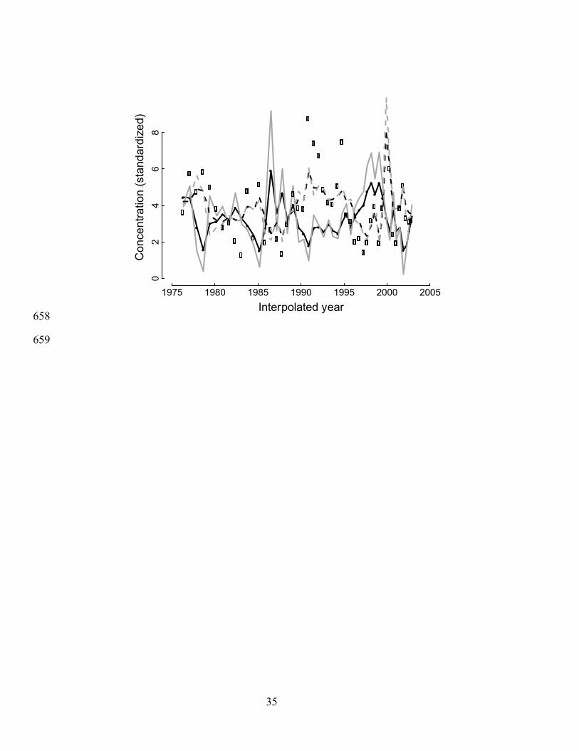
Diatoxanthin showed peaks in 1977, 1983, 1987, and 1999 that preceded peaks in midge 355

egg capsule counts (Fig. 2). This pattern is consistent with consumer-resource interactions in 356

which increases in diatoms occur at low midge abundance, and increases in midges occur at high 357

diatom abundance. In the state-space model (Eqs. 2, 3) the estimate for the effect of midges on 358

diatoxanthin is b12 = –0.90, and the effect of diatoxanthin on midges is b21 = 0.46 (Table 3); both 359

of these coefficients are significantly different from zero separately (b12: 21 = 13.08, P = 0.0003; 360

b21: 21 = 6.46, P = 0.011) and together (2

2 = 26.84, P < 0.0001). In addition, the analysis of 361

midge egg capsules and -carotene gave a negative estimate of b12 = –0.54 (21 = 9.79, P = 362

0.0017) and a positive estimate of b21 = 0.33 (21 = 4.04, P = 0.044), similar to but weaker than 363

the interactions inferred between midges and diatoxanthin. None of the other pigments showed 364

statistically significant values of b12 and b21, suggesting that the associated algae were not 365

18

involved in consumer-resource cycles (Table 3). Furthermore, the absence of significant 366

estimates if b12 and b21 for ubiquitous chlorophyll a confirms that models can be influenced by 367

post-depositional degradation of fossil records. 368

The state-space model fit to midge egg capsules and diatoxanthin gives information not 369

only about interaction strengths b12 and b21, but also about other properties inferred from the data. 370

The best-fitting state-space model (Table 3) gave an estimate of a = 0.55 (21 = 9.13, P = 0.0025). 371

This value of a implies that 0.50 of the diatoxanthin remained in the sediment stratum where it 372

was deposited, while 0.27 (= a/(1+a+a2+a3), 0.15, (= a2/(1+a+a2+a3) and 0.08 (= a3/(1+a+a2+a3) 373

represent sediment from slices 0.5, 1.0, and 1.5 cm below the observed core slice. This value of a 374

is similar for other pigments, except for the lower value estimated for echinenone. The fitted 375

value of b11 is close to zero, implying that there is little autocorrelation in diatom abundances 376

through time that is not explained by midge abundance; in contrast, b22 = 1.29, implying strong 377

autocorrelation in midge abundance. In contrast to these model parameters, other model 378

parameters were not informative. Specifically, the magnitudes of the process and sampling errors 379

(2i and 2

i) often traded off against each other, so that 2i > 0 and 2

i = 0, or 2i = 0 and 2

i > 0. 380

This is the result of the difficulty of statistically separating process error from measurement error. 381

To validate the state-space modeling approach, we simulated midge and diatom 382

abundance data using the model that had been fit to adult T. gracilentus data collected during 383

1977-2002 (Ives et al. 2008), and then simulated the sedimentation process including mixing 384

among layers (Appendix A). As we found for the real core data, the analysis of the simulated core 385

data identified a negative value of b12 = –0.55 and positive value of b21 = 0.82, both of which 386

were statistically significant. The simulations show that the state-space model (Eq. 2 and 3) is 387

19

robust to pronounced but complex (aperiodic) variation in population abundance caused by 388

consumer-resource interactions. 389

390

DISCUSSION 391

Paleoecological analysis of fossil midges (egg capsules) and diatoms (diatoxanthin) 392

provided direct support for the hypothesis that the dramatic midge population fluctuations in 393

Lake Mývatn are driven mainly by consumer-resource interactions between midges and their 394

food. Our state-space model showed that high midge egg capsule densities were associated with 395

decreases in diatoxanthin concentration and, in turn, high diatoxanthin concentrations were 396

associated with increases in midges. Furthermore, -carotene (algae) showed a similar though 397

weaker pattern, consistent with the fact that diatoms are a main component of the algal 398

assemblage, and that changes in concentration of diatoxanthin and -carotene were highly 399

correlated (Table 1). In contrast, none of other pigments showed significant correlation with 400

midge abundance. 401

Although concomitant changes in diatoms and midges do not prove that consumer-402

resource interactions underlie the observed decadal-scale population fluctuations, several lines of 403

evidence suggest that population fluctuations are not driven by other trophic interactions within 404

Lake Mývatn. Two other general possibilities are bottom-up effects on diatoms (i.e., some other 405

interaction drives diatom fluctuations, and midges follow) and top-down effects on midges (i.e., 406

some other interaction drives midge fluctuations, and diatoms follow). For the bottom-up 407

alternative, there would have to be a driver of diatom fluctuations other than midges. Diatoms are 408

the dominant group of primary producers in the lake, accounting for over 50% of primary 409

production (see Methods: Study system). Furthermore, most primary production is benthic rather 410

20

than pelagic, and diatoms are the dominant benthic primary producers (>95% of them are benthic 411

Fragilariaceae spp., Einarsson 1982). Thus, if there were an as yet unidentified driver of diatom 412

fluctuations, this driver would have to be strong enough to cause large fluctuations in benthic 413

primary production. Possible candidates for strong drivers are the mainly pelagic herbivore, 414

Daphnia longispina, and the epibenthic large-bodied cladocerans, and these do fluctuate in 415

synchrony with midges (Einarsson and Örnólfsdóttir 2004). Nonetheless, midges perform more 416

than 80% of the secondary production in the benthos (Lindegaard and Jónasson 1979), and 417

therefore are much better candidates for drivers of diatom abundance. Another possible candidate 418

for a driver of diatom fluctuations is Anabaena spp. that limit the growth of diatoms via shading. 419

Nonetheless, in the core data Anabaena spp. (as measured by echinenone) fluctuate in synchrony 420

with diatoms (diatoxanthin) (Table 1), which argues against shading from Anabaena spp. driving 421

diatom fluctuations. 422

The second general alternative hypothesis is that top-down forces generate fluctuations in 423

midges, and diatoms fluctuate in response. The obvious candidate for a top-down driver of midge 424

fluctuations is stickleback fish. Gut content analyses show that sticklebacks consume midges, 425

with midges comprising up to 56% of gut contents in a high-midge year and 9% in a low-midge 426

year (Gíslason et al. 1998). Nonetheless, the dominant midge, T. gracilentus, is better protected 427

than other midge species in their heavily constructed tubes and seems to be avoided by 428

sticklebacks. Furthermore, analyses of the time series of midges and sticklebacks (Einarsson et al. 429

2002) did not show the out-of-phase fluctuations that is expected for predator-prey cycles, instead 430

suggesting that sticklebacks follow rather than drive midge fluctuations. In addition to predators, 431

it is also possible that there is an unidentified parasite or pathogen that drives midge population 432

fluctuations, although we have little evidence for this. 433

Historical changes in grazing intensity and lake hydrology do not appear to have biased 434

21

the formation of the fossil record, nor the reliability of sedimentary time series as metrics of past 435

population abundance. Although intensification of herbivory is known to increase the rates of 436

deposition of algae and their pigments (Leavitt and Carpenter 1990), empirical (Leavitt et al. 437

1989) and modeling evidence (Cuddington and Leavitt 1999) show that this effect is limited to 438

less than a year in duration. Similarly, ecosystem-scale nutrient mass budgets reveal that over 439

90% of inflow silica is retained in the lake (Ólafsson 1979a), mainly due to uptake by and 440

deposition in diatoms (Opfergelt et al. 2011). 441

442

Statistical Methods 443

We developed a bootstrap method for determining the statistical significance of 444

correlations between two time series when each has temporal autocorrelation. Comparing its 445

results to standard correlations (Table 2) shows that standard correlations are likely to generate 446

type I errors (false positives). This can be explained simply with an example. Suppose there are 447

two 100-year time series that both show cycles with strict 10-year periods yet are independent. 448

There is a 20% chance that they fluctuate in either perfect synchrony or perfect asynchrony 449

(lagged by 5 years) for 100 years, which would clearly show very high statistical significance in a 450

standard correlation test; even if they were lagged by 1 or 6 years, the standard correlations 451

would likely be significant. Thus, it would be easy to get statistically significant correlations even 452

though we know that the time series are independent. Our bootstrap approach corrects for 453

autocorrelation and hence does not suffer from this potential source of type I errors. 454

Our state-space model takes a more-mechanistic approach, modeling explicit interactions 455

between variables and incorporating measurement error that accounts for sediment mixing. The 456

mathematical description of sediment mixing is simplistic, assuming that sediment layers below a 457

given strata have an influence that tapers off geometrically with depth. This is similar to the 458

22

assumption used by Blaauw and Christen (2011) to construct a model relating sediment depth to 459

age determined by radiocarbon dating. Nonetheless, there are numerous bioturbation (Kristensen 460

et al. 2012) models that incorporate much more sophisticated assumptions about the physical and 461

biological processes underlying sediment mixing (Sandnes et al. 2000, Meysman et al. 2005, 462

Schiffers et al. 2011). We have not attempted to incorporate the complexities of bioturbation into 463

our model, because the information needed to apply these approaches is unknown for our system. 464

Therefore, our approach matches the level of detail in the model to the data we have. When 465

applied to simulated data (Appendix A, online Supplemental Material), the approach did identify 466

the effects of sedimentation in smoothing the fluctuations in deposition rates. Despite this 467

smoothing effect, the state-space model still identified strong interactions between midges and 468

diatoms in both simulated and real data. 469

470

Conclusion 471

Our analyses of sediment core data give strong support to the midge-diatom consumer-472

resource hypothesis to explain the fluctuations in midge and diatom abundances in Lake Mývatn. 473

Sediment cores are the only source of information about diatom fluctuations in Lake Mývatn, 474

because continuous long-term monitoring was not performed. Our example thus illustrates the 475

benefits of paleoecology to reconstruct history and extract missing information that is preserved 476

in sediment cores. This information is not limited to broad, ecosystem-level processes, but can 477

also be used to understand the population dynamical interactions between species. 478

479

ACKNOWLEDGMENTS 480

We thank Eva Pier for field assistance and Theodóra Matthíasdóttir for lab work. Two 481

anonymous reviewers provided great suggestions that improved this work. The study was funded 482

23

by the European Union “Eurolimpacs”-project GOCE-CT-2003-505540 and by Icelandic Centre 483

for Research (RANNÍS) grants no. 050219032 and 080010008. PL acknowledges funding from 484

NSERC (Natural Science and Engineering Research Council of Canada) and funding for ARI 485

was provided in part by US-NSF-DEB-LTREB-1052160. 486

487

REFERENCES 488

Aaby, B., and B. E. Berglund. 1986. Characterisation of peat and lake deposits. Pages 231-246 in 489

B. E. Berglund, editor. Handbook of Holocene Palaeoecology and Palaeohydrology. John 490

Wiley and Sons, Chichester, NY. 491

Berryman, A. A. 1976. Theoretical explanation of mountain pine beetle dynamics in lodgepole 492

pine forests. Environmental Entomology 5:1225-1233. 493

Berryman, A. A., G. D. Amman, and R. W. Stark. 1978. Theory and practice of mountain pine 494

beetle management in lodgepole pine forests. Forest, Wildlife and Range Experimental 495

Station, University of Idaho, Moscow, Idaho, USA. 496

Blaauw, M., K. D. Bennett, and J. A. Christen. 2010. Random walk simulations of fossil proxy 497

data. Holocene 20:645-649. 498

Blaauw, M., and J. A. Christen. 2011. Flexible paleoclimate age-depth models using an 499

autoregressive gamma process. Bayesian Analysis 6:457-474. 500

Box, G. E. P., G. M. Jenkins, and G. C. Reinsel. 1994. Time series analysis: forecasting and 501

control. Third edition. Prentice Hall, Englewood Cliffs, New Jersey, USA. 502

Brinkhurst, R. O., K. E. Chua, and E. Batoosingh. 1969. Modifications in sampling procedures as 503

applied to studies on the bacteria and tubificid oligochaetes inhabiting aquatic sediments. 504

Journal of the Fisheries Research Board of Canada 26: 2581-2593. 505

24

Carpenter, S. R., and P. R. Leavitt. 1991. Temporal variation in a paleolimnological record 506

arising from a trophic cascade. Ecology 72: 277-285. 507

Cuddington, K., and P. R. Leavitt. 1999. An individual-based model of pigment flux in lakes: 508

Implications for organic biogeochemistry and paleoecology. Canadian Journal of 509

Fisheries and Aquatic Science 56: 1964-1977. 510

Dennis, B., and B. Taper. 1994. Density dependence in time series observations of natural 511

populations: estimation and testing. Ecological Monographs 64:205-224. 512

Dwyer, G., J. Dushoff, and S. H. Yee. 2004. The combined effects of pathogens and predators on 513

insect outbreaks. Nature 430:341-345. 514

Efron, B., and R. J. Tibshirani. 1993. An introduction to the bootstrap. Chapman and Hall, New 515

York. 516

Einarsson, Á. 1982. The paleolimnology of Lake Myvatn, northern Iceland: plant and animal 517

micro-fossils in the sediment. Freshwater Biology 12:63-82. 518

Einarsson, Á., A. Gardarsson, G. M. Gíslason, and A. R. Ives. 2002. Consumer-resource 519

interactions and cyclic population dynamics of Tanytarsus gracilentus (Diptera: 520

Chironomidae). Journal of Animal Ecology 71:832-845. 521

Einarsson, Á., and R. D. Gulati, editors. 2004. Ecology of Lake Myvatn and the River Laxa: 522

temporal and spatial variation. 523

Einarsson, Á., and E. B. Örnólfsdóttir. 2004. Long-term changes in benthic Cladocera 524

populations in Lake Myvatn, Iceland. Aquatic Ecology 38:253-262. 525

Einarsson, Á., G. Stefánsdóttir, H. Jóhannesson, J. S. Ólafsson, G. M. Gíslason, I. Wakana, G. 526

Gudbergsson, and A. Gardarsson. 2004. The ecology of Lake Myvatn and the River Laxa: 527

Variation in space and time. Aquatic Ecology 38:317-348. 528

25

Gardarsson, A., Á. Einarsson, G. M. Gíslason, T. Hrafnsdóttir, H. R. Ingvason, E. Jónsson, and J. 529

S. Ólafsson. 2004. Population fluctuations of chironomid and simuliid Diptera at Myvatn 530

in 1977-1996. Aquatic Ecology 38:209-217. 531

Gíslason, G. M., A. Gudmundsson, and Á. Einarsson. 1998. Population densities of the three-532

spined stckleback (Gasterosteus aculeatus L.) in a shallow lake. Verh Internat Verein 533

Limnol 26:2244-2250. 534

Håkanson, L., and M. Jansson. 1983. Principles of lake sedimentology. Springer, New York, NY. 535

Harvey, A. C. 1989. Forecasting, structural time series models and the Kalman filter. Cambridge 536

University Press, Cambridge, U.K. 537

Hauptfleisch, U., Á. Einarsson, T. J. Andersen, A. Newton, and A. Gardarsson. 2012. Matching 538

thirty years of ecosystem monitoring with a high resolution microfossil record. 539

Freshwater Biology 57:1986-1997. 540

Holm, S. 1979. A simple sequentially rejective multiple test procedure. Scandinavian Journal of 541

Statistics 6:65-70. 542

Ingvason, H. R., J. S. Ólafsson, and A. Gardarsson. 2004. Food selection of Tanytarsus 543

gracilentus larvae (Diptera: Chironomidae): an analysis of instars and cohorts. Aquatic 544

Ecology 38:231-237. 545

Ives, A. R., K. C. Abbott, and N. L. Ziebarth. 2010. Analysis of ecological time series with 546

ARMA(p,q) models. Ecology 91:858-871. 547

Ives, A. R., Á. Einarsson, V. A. A. Jansen, and A. Gardarsson. 2008. High-amplitude fluctuations 548

and alternative dynamical states of midges in Lake Myvatn. Nature 452:84-87. 549

Jónasson, P. M., editor. 1979. Ecology of eutrophic, subarctic Lake Myvatn and the River Laxa. 550

Oikos. 551

26

Jónasson, P. M., and H. Adalsteinsson. 1979. Phytoplankton production in shallow eutrophic 552

Lake Myvatn, Iceland. Oikos 32:113-138. 553

Kendall, B. E., C. J. Briggs, W. W. Murdoch, P. Turchin, S. P. Ellner, E. McCauley, R. M. 554

Nisbet, and S. N. Wood. 1999. Why do populations cycle? A synthesis of statistical and 555

mechanistic modeling approaches. Ecology 80:1789-1805. 556

Krebs, C. J. 2011. Of lemmings and snowshoe hares: the ecology of northern Canada. 557

Proceedings of the Royal Society B-Biological Sciences 278:481-489. 558

Krebs, C. J., S. Boutin, R. Boonstra, A. R. E. Sinclair, J. N. M. Smith, M. R. T. Dale, K. Martin, 559

and R. Turkington. 1995. Impact of food and predation on the snowshoe hare cycle. 560

Science 269:1112-1115. 561

Kristensen, E., G. Penha-Lopes, M. Delefosse, T. Valdemarsen, C. O. Quintana, and G. T. Banta. 562

2012. What is bioturbation? The need for a precise definition for fauna in aquatic 563

sciences. Marine Ecology Progress Series 446:285-302. 564

Leavitt, P. R., and S. R. Carpenter. 1989. Effects of sediment mixing and benthic algal 565

production on fossil pigment stratigraphies. Journal of Paleolimnology 2:147-158. 566

Leavitt, P. R., S. R. Carpenter and J. F. Kitchell. 1989. Whole-lake experiments: The annual 567

record of fossil pigments and zooplankton. Limnology and Oceanography 34: 700-717. 568

Leavitt, P. R., and D. A. Hodgson. 2001. Sedimentary pigments. Pages 295-325 in J. P. Smol, H. 569

J. B. Birks, and W. M. Last, editors. Tracking environmental change using lake 570

sediments. V. 3: Terrestrial, algal and siliceous indicators. Kluwer, Dordrecht, the 571

Netherlands 572

Lindegaard, C., and P. M. Jónasson. 1979. Abundance, population dynamics and production of 573

zoobenthos in Lake Mývatn, Iceland. Oikos 32:202-227. 574

Lotka, A. J. 1925. Elements of physical biology. Williams and Wilkins, Baltimore, MD. 575

27

McCauley, E., W. A. Nelson, and R. M. Nisbet. 2008. Small-amplitude cycles emerge from 576

stage-structured interactions in Daphnia-algal systems. Nature 455:1240-1243. 577

McCauley, E., R. M. Nisbet, W. W. Murdoch, A. M. de Roos, and W. S. C. Gurney. 1999. Large-578

amplitude cycles of Daphnia and its algal prey in enriched environments. Nature 402:653-579

656. 580

Meysman, F. J. R., B. P. Boudreau, and J. J. Middelburg. 2005. Modeling reactive transport in 581

sediments subject to bioturbation and compaction. Geochimica et Cosmochimica Acta 582

69:3601-3617. 583

Murdoch, W. W., R. M. Nisbet, E. McCauley, A. M. deRoos, and W. S. C. Gurney. 1998. 584

Plankton abundance and dynamics across nutrient levels: Tests of hypotheses. Ecology 585

79:1339-1356. 586

Myers, J. H. 1988. Can a general hypothesis explain population cycles of forest Lepidoptera? 587

Advances in Ecological Research 18:179-242. 588

Ólafsson, J. 1979a. The chemistry of Lake Mývatn and River Laxá. Oikos 32:82-112. 589

Ólafsson, J. 1979b. Physical characteristics of Lake Mývatn and River Laxá. Oikos 32:38-66. 590

Opfergelt, S., E. S. Eiríksdóttir, K. W. Burton, Á. Einarsson, C. Siebert, S. R. Gíslason, and A. N. 591

Halliday. 2011. Quantifying the impact of freshwater diatom productivity on silicon 592

isotopes and silicon fluxes: Lake Myvatn, Iceland. Earth and Planetary Science Letters 593

305:73-82. 594

Patoine, A., and P. R. Leavitt. 2006. Century-long synchrony of algal fossil pigments in a chain 595

of Canadian prairie lakes. Ecology 87:1710-1721. 596

Sandnes, J., T. Forbes, R. Hansen, B. Sandnes, and B. Rygg. 2000. Bioturbation and irrigation in 597

natural sediments, described by animal-community parameters. Marine Ecology Progress 598

Series 197:169-179. 599

28

Schiffers, K., L. R. Teal, J. M. J. Travis, and M. Solan. 2011. An Open Source Simulation Model 600

for Soil and Sediment Bioturbation. PLoS ONE 6. 601

Schnurrenberger, D., J. Russell, and K. Kelts. 2003. Classification of lacustrine sediments based 602

on sedimentary components. Journal of Paleolimnology 29:141-154. 603

Smol, J. P. 2010. The power of the past: using sediments to track the effects of multiple stressors 604

on lake ecosystems. Freshwater Biology, 55: 43-59. 605

Stenseth, N. C. 1999. Population cycles in voles and lemmings: density dependence and phase 606

dependence in a stochastic world. Oikos 87:427-461. 607

Thorarinsson, S. 1979. The postglacial history of the Mývatn area. Oikos 32:17-28. 608

Thorbergsdóttir, I. M., S. R. Gíslason, H. R. Ingvason, and Á. Einarsson. 2004. Benthic oxygen 609

flux in the highly productive subarctic Lake Myvatn, Iceland: In situ benthic flux chamber 610

study. Aquatic Ecology 38:177-189. 611

Troels-Smith, J. 1955. Karakterisering af løse jordarter. Danmarks Geologiske Undersøgelse, 612

Copenhagen. 613

Turchin, P. 2003. Complex population dynamics: a theoretical/empirical synthesis. Princeton 614

University Press, Princeton, NJ. 615

Turchin, P., and I. Hanski. 2001. Contrasting alternative hypotheses about rodent cycles by 616

translating them into parameterized models. Ecology Letters 4:267-276. 617

Turchin, P., S. N. Wood, S. P. Ellner, B. E. Kendall, W. W. Murdoch, A. Fischlin, J. Casas, E. 618

McCauley, and C. J. Briggs. 2003. Dynamical effects of plant quality and parasitism on 619

population cycles of larch budmoth. Ecology 84:1207-1214. 620

621

APPENDIX A 622

29

Simulation of midge and diatom abundance data. 623

624

APPENDIX B 625

Stratigraphy of pigments, loss on ignition (LOI), C, N, 13C, diatoms, chironomid eggs and 626

Cladocera exuviae in the sediment cores. 627

628

30

Table 1: Correlations among six variables from two sediment cores. 629

Midge

eggs Dia Echin Allox -caro

Diatoxanthin -0.37*

Echinenone -0.16 0.42*

Alloxanthin -0.03 0.25 0.34*

-carotene -0.19 0.64**†† 0.52** –0.01

Chlorophyll-a 0.09 0.53* 0.53* 0.17 0.77**††

630 * P < 0.05, ** P < 0.01, calculated from a bootstrap that incorporates autocorrelation (Eq. 1) 631

† P < 0.05, †† P < 0.01, calculated from a bootstrap Holm-Bonferroni correct for multiple 632

comparisons that incorporates autocorrelation (Eq. 1) 633

634

635

31

Table 2: P-values (2-tailed and not corrected for multiple comparisons) from a standard Pearson 636

correlation test (upper-right triangle) and from the bootstrap (Eq. 1) that accounts for temporal 637

autocorrelation (lower-left triangle). 638

Midge

eggs Dia Echin Allox -caro

Chl-a

Midge eggs 0.012 0.29 0.87 0.20 0.52

Diatoxanthin 0.039 0.002 0.08 0.0000 0.0000

Echinenone 0.35 0.018 0.016 0.0001 0.0000

Alloxanthin 0.88 0.19 0.046 0.98 0.23

-carotene 0.27 0.0001 0.003 0.96 0.0000

Chlorophyll-a 0.67 0.011 0.011 0.43 0.0003

639

32

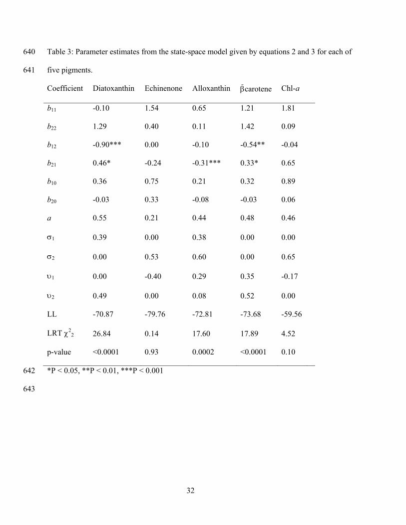
Table 3: Parameter estimates from the state-space model given by equations 2 and 3 for each of 640

five pigments. 641

Coefficient Diatoxanthin Echinenone Alloxanthin carotene Chl-a

b11 -0.10 1.54 0.65 1.21 1.81

b22 1.29 0.40 0.11 1.42 0.09

b12 -0.90*** 0.00 -0.10 -0.54** -0.04

b21 0.46* -0.24 -0.31*** 0.33* 0.65

b10 0.36 0.75 0.21 0.32 0.89

b20 -0.03 0.33 -0.08 -0.03 0.06

a 0.55 0.21 0.44 0.48 0.46

1 0.39 0.00 0.38 0.00 0.00

2 0.00 0.53 0.60 0.00 0.65

1 0.00 -0.40 0.29 0.35 -0.17

2 0.49 0.00 0.08 0.52 0.00

LL -70.87 -79.76 -72.81 -73.68 -59.56

LRT 22 26.84 0.14 17.60 17.89 4.52

p-value <0.0001 0.93 0.0002 <0.0001 0.10

*P < 0.05, **P < 0.01, ***P < 0.001 642

643

33

644

Fig. 1: Detrended sediment core data for midge egg capsules and diatoxanthin, echinenone, 645

alloxanthin, -carotene, and chlorophyll-a (dots). Smoothing of midge (gray lines) and pigment 646

data (black lines) was performed to make fluctuating patterns in the data more clear; a direct form 647

II transposed filter was used with numerator coefficients (0.25, 0.5, 0.25), and denominator 648

coefficient 1. 649

650

Fig. 2: Fit of the state-space model (Eqs. 2, 3) to detrended diatoxanthin (solid dots) and midge 651

egg capsule abundance (open dots). Solid and dashed black lines give the fit of the model to the 652

observed values x*(t) and u*(t) of diatoxanthin and midges (Eq. 3), whereas the solid and dashed 653

gray lines give the estimates of the deposition rates prior to sediment mixing (Eq. 2).654

34

655

656

657

Diatoxanthin

−2

02

● ●

●

●

● ●

●

●

●

●

●

●

●

●

●

●

●

●

●

●

●

●

● ●●

●

●●

●

●

●

●

●●

●

●

●

●

●

●

●

●

●●

●●

●

●

Echinenone

−2

02

●

●

●

●

●●

●

●

●

●

●

●

●

●●

●

●

●

●

●

●

●

●

●

●

●

●

●

●●

●

●

●

●

●

●

●

●

●

●

●

●

●

●

● ●

●

●

Alloxanthin

−2

02

●

●

●

●

●

● ● ●

●

● ● ●

●

●

●

●

●

●

●●

●

●

●●

●

●

●

●

●

●

●

●

●

●

●

● ●● ●

●

●

●

●

●

● ●

●●

Beta−carotene

−2

02

●

● ● ●

●

●●

●

● ●

●

● ●●

●

●

● ●●

●

●

●

●

● ●

●

●

●

●

●

●●

●

●

●

●●

●

●

●

●

●

●

●

● ●●

●

Chlorophyll−a

0 10 20 30 40 50

−2

02

●●

●

●●

●

●●

●● ●

●

●●

●

●●

● ●●

●

●

●

●

●

●●

●

●● ● ●

●

●

●

●

●●

● ●

●

●

●

●

● ●●

●

Sample (time)

Con

cent

ratio

n (s

tand

ardi

zed)

35

658

659

● ●

●

●

● ●●●

●

●●

●

●

●

●

●

●

●

●

●●

●

● ●●●● ●

●

●

●

●●●

●

●

●

●

●

●

●

●

●●

●●

●

●

TT

d[, 2

]

1975 1980 1985 1990 1995 2000 2005

02

46

8

Interpolated year

Co

ncen

trat

ion

(sta

ndar

dize

d)

36

660