identifying components of effective mathematics … mathematics program components i ... three...
TRANSCRIPT

Final Report—R215U010023
Identifying Components of Effective
Mathematics Programs
Prepared for the University of Oregon
by
Laurence A. Toenjes, Ph.D., Toenjes & Associates
Jeffrey C. Lewis, Ph.D., Pitzer College
Mara B. Winick, Ph.D., University of Redlands
December, 2004
This study was performed under a contract with the University of Oregon, with funding
provided by the US Department of Education (grant number R215U010023).
Portions of the data and analysis pertaining to State of Texas’ schools and school districts
relied upon a study funded by the Texas Education Agency and the Texas Region IV
Education Service Center.

Effective Mathematics Program Components
i
Table of Contents
Executive Summary ii
Section 1: Introduction and Purpose 1
Section 2: Overview of study and the Ten Components of Effective Schools 3
Section 3: Survey Design, Format, and Procedures 10
Section 4: Selection of School Districts and the Use of Hierarchical
Linear Models (HLM) 12
Section 5: Analysis of California Survey Data 19
Section 6: Analysis of North Carolina Survey Data 39
Section 7: Analysis of Texas Survey Data 53
Section 8: Relationship between student performance, proportion of
economically disadvantaged students, and test difficulty—three states 68
Section 9: Multi-state analysis—California, North Carolina, and Texas 76
Section 10: Summary and Conclusions 84
Bibliography 91
Appendix: Survey Forms 92
Endnotes 127

Effective Mathematics Program Components
ii
Executive Summary
Previous work has identified Ten Components of Effective Schools which were often
associated with schools and school districts whose students were achieving above
average academically. The main purpose of this study was to determine if a
questionnaire-based data gathering process could capture information sufficient to test the
efficacy of these Ten Components upon mathematics performance in elementary and
middle schools. That is, can a short questionnaire filled out by teachers and
administrators adequately capture sufficient information about such characteristics as
administrative practices, curriculum alignment and professional development to test
whether different degrees or quality of implementation of these practices actually makes
any difference in educational outcomes at the school or school district level?
Information was obtained from 828 teachers in 104 schools located in 18 school
districts across three states—California, North Carolina, and Texas. Several districts in
each state and several schools within each district were selected which had large
proportions of economically disadvantaged students. In addition, it was attempted to get a
mix of districts which exhibited either higher than average or lower than average
performance among the majority of their campuses, using a criterion described in the
paper.
Correlation and linear regression analyses were used to see which of the Ten
Components were associated with the more successful schools, leaving aside district
influence. Using Hierarchical Linear Models (HLM) analysis, the district-level
aggregates derived from the survey data were used to determine which of the components
were most strongly associated with higher than predicted performance among the school
districts in the sample.
Strong and consistent correlations were found between school-wide average student
math performance and the degree of implementation of several of the Ten Components.
The survey results were even more effective in explaining variations in the average math
performance of entire school districts, even when correcting for differences in the
proportion of economically disadvantaged students.
The results were weakest based upon data for North Carolina. Reasons for this are
discussed.

Effective Mathematics Program Components
iii
The data from all three states were also combined, making the statistical results even
stronger. Problems inherent in combining such data obtained from different states, each
administering a different standardized test, are discussed and dealt with.
The school level performance data for California schools were available based on
three different passing criteria—Below Basic, Basic, and Proficient. Greater predictive
power of the Ten Components was associated with the more demanding assessment
criteria, but the passing rates were lower. This suggests that there may be a tradeoff
between state tests designed to maximize research potential and tests used to publicly
label schools for accountability purposes.
It is concluded that the survey instrument used to gather data for this study is indeed
effective in measuring the degree to which school district and school practices are aligned
with the Ten Components. It is also concluded that the degree of implementation of at
least several of the Ten Components is strongly associated with differences in average
student performance, both at the school and the school district levels.
The results for school districts makes clear that the district role goes beyond merely
providing infrastructure and services for their schools. District administrations also have
a central role in bringing about higher student performance in all schools within their
jurisdiction. These findings suggest caution in the face of calls for arbitrarily limiting the
proportion of district dollars that can be spent for district administration functions. These
findings also suggest caution with respect to certain proposals for directly funding
schools from the state level, bypassing the district altogether.

Effective Mathematics Program Components
1
Section 1: Introduction and Purpose
Closing the gap in school performance between students in different economic, ethnic
and racial groups is perhaps the major challenge facing US education today. From one
perspective the lower average academic performance by minority and economically
disadvantaged students represents a major economic loss to the nation as a whole, and
certainly translates into a lifetime of lower earnings for most of the underachievers.
From another perspective, the differential rates in average academic achievement by the
different ethnic, racial, and economic groups in the US translates into a tragic
postponement of attaining one of the most cherished values of this nation—that all
persons are created equal and have equal opportunity to achieve the benefits that this
nation has to offer and to have equal voice in its affairs. This goal cannot be reached as
long as such glaring discrepancies in school achievement exist among the different major
socioeconomic groups.
It was hoped that the elimination of legally segregated schools would eventually
reduce if not eliminate inter-group differences in school performance. Certainly there has
been progress, but data collected in recent decades continue to show large differences.
As a result there has been a new surge of efforts to reform and improve education across
the United States. The report A Nation at Risk (National Commission on Excellence in
Education, 1983) is often cited as providing the stimulus for these efforts. Perhaps aided
in a significant way by the advent of economical computerized record-keeping and data-
retrieval technology, reform efforts have been accompanied by an expansion in student
testing. This increase in testing by schools and school districts in most states has
provided the means to constantly monitor the performance and progress of all students in
very detailed fashion. These data have given new emphasis to the issue of disparities in
school performance among various ethnic, racial, and economic groups as these
differences are now documented in great detail and their relative magnitudes recorded
annually.
Clear, graphic documentation of the performance gaps following from the widespread
availability of test-based performance data has been accompanied by widespread
adoption of statewide accountability systems. These systems have been designed to

Effective Mathematics Program Components
2
focus attention on low performing schools and to try to bring about improvements in their
performance. One of the expected benefits of these accountability systems is the
potential to identify schools and school districts that exhibit outstanding performance, to
determine the factors contributing to the higher performance, and to encourage the lower
performers to adopt similar practices.
Research that helps to close this gap by determining which school characteristics
relate to improved performance is sorely needed, but in many areas, and in particular
when focused on mathematics instruction, there is not a large body of reliable findings to
direct educators. A recent report from the National Research Council (2001) noted the
limited availability of experimental research related to determining methods that raise
academic achievement, while another report from the What Works Clearinghouse (2004)
highlights the lack of a research basis for most mathematics programs.
The purpose of this study is to use data generated by statewide accountability systems
to explore mathematics assessment performance and to differentiate among schools and
school districts based upon the implementation of particular practices at various
organizational levels. Starting from prior work, the current study will explore the
relationship between instructional characteristics and practices that may help explain the
differences between high and low performing schools. Interviews and questionnaires
were used to gather site-specific and district data from school districts, associated campus
leaders and teachers to help identify such effective practices. However, this effort should
be viewed only as a pilot study because of the relatively small numbers of school districts
included.
The original funding for this study was intended to permit data collection within two
states. As the work in California and North Carolina was being organized however,
support was obtained from the State of Texas (Regional Service Center IV) to carry out a
similar study within Texas, also focusing on mathematics.
The report that follows describes and utilizes the data gathered across the three states.
Section two outlines the conceptual definitions by which the study questionnaire was
designed. Section three details the survey development process and data collection
including sampling, survey administration and participation stipends. In Section 4 the use
of Hierarchical Linear Models (HLM) is described, especially as used in selecting

Effective Mathematics Program Components
3
districts in each state to be included in the study. In Sections 5, 6, and 7 the survey data
results are analyzed for each of California, North Carolina, and Texas, respectively. In
Section 8 data from California are used to demonstrate how different passing rate
thresholds used to determine student success on the state’s standardized tests can affect
the usefulness of the reported data for research purposes. Section 9 presents a brief
analysis based upon the data for all three states, taking advantage of the larger sample
size. There is also a discussion of some of the problems inherent in the use of multi-state
data. Finally, a summary and conclusions are presented in Section 10.
Section 2: Overview of the study and the Ten Components of Effective Schools
The practices assessed in carrying out the purpose of this study are referred to as The
Ten Components of Effective Schools, or the Ten Components, for short. The efficacy of
the Ten Components for improving performance will be tested here with student
performance measures for elementary and middle school mathematics collected in three
different states—California, North Carolina, and Texas. All of these states have been
involved in comprehensive statewide testing of all students in grades 3 through 8, and
have incorporated the testing regime into their respective accountability systems.
The content framework for the practices considered was modeled on a study carried
out earlier in Texas, but which focused on test results in reading (Toenjes & Garst, 2002).
This study involved assessing the same Ten Components upon which this current study
focuses, but with campus reading results on the Texas Assessment of Academic Skills
(TAAS; see http://www.tea.state.tx.us/student.assessment/ for a full description of
TAAS) as the dependent variable. Most of the data for the Texas study were obtained by
expert interviewers using a structured interview instrument tailored to each of the three
institutional levels—teachers, school principals and reading coordinators, and district
superintendents and curriculum specialists. The original interview instruments were
designed to assess the degree of implementation of each of the Ten Components at each
level: the school, principal and district. This study, however, focuses specifically on
mathematics performance as impacted by the three levels of practice and does so across
three states with mature accountability systems in place. This math study differs from the
reading study by the sampling of a more geographically diverse population of schools

Effective Mathematics Program Components
4
and by the data collection process. Administered surveys rather than expert interviewing
were used to reach the broader state samples in a more timely and economic fashion that
allowed for more uniform assessment.
The procedures and results from California, North Carolina and Texas are reported in
separate sections (Sections 5, 6, and 7, respectively) and the results then compared. In the
final sections of this report the data will be pooled, thus providing a larger number of
observations with which to test certain hypotheses. It will also provide an opportunity to
better understand the problems inherent in such data mergers. A discussion of data
compatibility is included and the method used to transform the campus student
performance data from the three states into compatible measures is described. In addition,
the inclusion of certain data from Texas, combined with the corresponding data from
North Carolina and California, may provide insights into some of the issues which will
arise with the interstate comparison of student performance data based upon different
assessment regimes (discussed in Sections 8 and 9).
Ten Components of Effective Schools
The Texas Education Agency (TEA) has promoted a list of ten characteristics that it
maintains are implemented in whole or in part at the most successful schools in Texas.
As already mentioned, the list of these components was formalized by Dr. Doug
Carnine1. Anecdotal observations and some preliminary studies support the contention
that adoption of these practices contribute to school success. The description of the ten
components from the Texas Education Agency (TEA) website is reproduced below (see
http://www.tea.state.tx.us/math/TenComEffSch.htm; note that the components here are in
a different order to reflect our data coding).
While many factors contribute to the overall success of mathematics instruction,
studies show that effective math instruction for all students requires a total school effort
and cannot be accomplished without the active, knowledgeable support of school
administrators at both the district and campus level. Factors that contribute to the success
for all students in mathematics include the following:

Effective Mathematics Program Components
5
1. Sound Administrative Practices: District leaders prioritize resources to
support an effective mathematics program capable of bringing all students to high
levels of performance.
Communicate the expectation that achievement for all students will
replicate that of the highest performing schools with comparable students.
Translate expectations into specific goals. Leaders provide
acknowledgement to those who achieve high levels of student
achievement.
Structure the administrative role as supporting instruction rather than
enforcing compliance. Administrators work with school teams to plan and
support improvement in performance. Prioritize district and campus
budgets so that needed resources are available for all components of the
math program such as: lead teachers, materials, and/or teachers to provide
supplemental instruction.
District and campus leaders take actions as necessary to ensure adequate
student progress and monitoring. The math program is monitored through
visits to schools and/or classrooms and analysis of student assessment
data. Leaders have adequate time and/or staff to accomplish this goal.
Create an environment conducive to instruction and success. For example:
campuses initiate a proactive school-wide management program to
facilitate cooperative and responsible behavior from students. A
motivational system is in place for all students- those struggling and those
who do well. Students are placed where they will succeed and the system
encourages student performance and effort.
2. Aligned Curriculum: The curriculum is aligned between the Texas Essential
Knowledge and Skills, teaching objectives, textbooks, materials, and assessment.
3. Ongoing Assessment and Planning: Student learning is assessed throughout
the school year and results are used to plan and group students for instruction and
to provide feedback to students and parents.
4. Immediate Intervention for Students Experiencing Difficulty Mastering
Concepts: Students who experience difficulty are identified in a timely manner
and intensive interventions are designed to remediate their deficiencies. Extra
instruction targets their specific instructional needs.
5. Increased and Effective Use of Instructional Time: Sufficient time is
designated for math instruction each day to ensure that all students reach high
levels of achievement in mathematics. 60 to 90 minutes per day is allotted for
students performing at or above grade level and additional instructional time is
allotted for students having difficulty mastering math concepts. Additional
instructional time is provided through before/after school classes, tutoring,
Saturday classes, summer programs, and extra instruction during the school day in
small group settings.

Effective Mathematics Program Components
6
6. Teacher Knowledge of Mathematics Content: Teachers have a good, clear
understanding of the mathematics content they teach and are carefully selected for
their teaching assignments.2
7. Instructional Materials and Teaching Techniques: Instructional materials
and techniques are part of a carefully planned math program that is structured to
meet the individual needs of students. These instructional materials are consistent
with what is used in districts with high levels of achievement in math.
8. Differentiated Instruction: Schools and classrooms are organized so that
students with similar needs receive effective instruction through flexible skill
grouping.
9. Focused Professional Development: Professional Development is an on-going
priority and is focused intensely on student needs identified through TAAS3 and
district assessments.
10. End-of-Year Analysis of Student Performance: End-of-year student
performance is measured with state and/or national tests to analyze program
effectiveness.
Gather data from the beginning and end of the school year on a variety of
assessment instruments, including TAAS, to determine program
effectiveness and make plans for yearly improvement efforts.
Compare campus performance on TAAS with comparable higher
performing schools to set expectations for improvement efforts.
Establish communication links between elementary, middle and high
school regarding student preparation for Algebra 1. Determine which
concepts, if any, need more attention at each level.
Previous Studies
Work exploring these ten components has shown promise in more limited
explorations completed in recent years. Toenjes and Garst (2000) set out to determine
whether eight district practices were associated with district average student math
performance. The major practices included district administration, academic oversight of
campuses, accountability for administrators, curriculum alignment with state standards,
implementation of remediation for low-performing students, and alignment of
professional development with student performance on state standardized tests. Teachers,
school administrators, and district administrators were interviewed by the same

Effective Mathematics Program Components
7
interviewer, their responses to specific questions analyzed and compared, and finally a
single score established for each district. This score was intended to represent the
relative extent to which all 8 practices had been implemented in each district. When the
districts were rank-ordered on the basis of their scores, those with higher scores had
received the State of Texas accountability rating of Recognized, whereas those with
lower total scores received the lower Acceptable rating.
A number of qualitative findings were also reported in this study. These included
the following:
All middle schools and high schools surveyed reported that alignment team
meetings across grades and campuses are taking place. The frequency and
agendas of these meetings vary from general discussions about campus
problems to in-depth coordination of curriculum designs.
Five of the 16 middle school campuses visited have hired experienced math
teachers to fill instructional specialist positions in math.
Three of the 25 campuses visited free teachers for 2 periods a day; one for
routine conference duties and one for math teacher meetings.
All but two of the 9 high schools visited provide to low-performing students at
least 90 minutes of math per day extending throughout the entire school year.
Teachers and administrators track scores of low-performing students very
closely on some campuses. On other campuses no records are kept.
On some campuses in some districts giving up an elective is required for
students who are identified as low-performing.
On other campuses some administrators interviewed stated it is not possible to
have mandatory programs for low-performing students because constraints
imposed by electives and sports are impossible to overcome.
For the 15 middle school campuses visited, which had consistent attendance
boundaries the last two years, enrollment in Algebra I has increased by 46
percent in the current school year as compared to last year.4
This study involved only 8 Texas school districts. While the study was not
designed to determine the association between any individual practice and improved
student performance, on average a greater degree of implementation of these practices

Effective Mathematics Program Components
8
was associated, for the entire district, with higher state accountability ratings. In short,
these practices might be called the Eight Components of Effective Districts.
In ―Survey of Texas Reading Programs Based on the Ten Components of Best
Practice, Grades K-8‖, Toenjes and Garst (2002) attempted to determine if a greater
degree of implementation of each of the Ten Components of Effective Schools identified
by Carnine was associated with better student reading performance. Data were collected
from 8 school districts, and 52 schools and 104 teachers in those districts. The criterion
for selecting districts was based on a district-wide measure reflecting average pass rates
on the State of Texas’ TAAS reading test, correcting for the proportion of economically
disadvantaged students attending the various campuses in each district. One of the Ten
Components, component 9 (Focused Professional Development, which means promoting
teacher collaboration and training based on student performance), was found to be
statistically significant. One of the elements within component 1 (Sound Administrative
Practices) was significant when used alone. This component was the degree to which
individual school principals were granted certain budgetary authority.
Both of the factors found to be associated with improved district-wide student
performance, corrected for poverty, are activities that are likely best organized and
instituted by the district administration. Certainly delegation of budgetary authority can
only occur with district approval, and teacher professional development is normally a
district function. In addition to negative effects of larger proportions of economically
disadvantaged students, it was also found that a measure of high student mobility among
campuses dampened average school performance. In Texas students who change
campuses frequently while remaining in the same district must be included in the end-of-
year accountability test results.
Another study that attempted to use accountability system data to identify
effective school practices is reported by Thomas, Warren + Associates (2003), hereafter
TWA. This Massachusetts study focused on improvement over time. Only schools were
included which had administered the MCAS test each year for the previous four years to
at least 50 students. Schools which had demonstrated above average increases in the
proportion of students in the Proficient and Advanced mathematics MCAS levels and
also above average rates of decrease in the percent of students in the Warning level were

Effective Mathematics Program Components
9
designated as IPAW schools. Those in the sample not meeting these requirements were
thus the non-IPAW schools. There were 213 schools studied altogether, with 71 being
IPAW schools, of which 65 actually participated. Various school practices and
characteristics were noted with the goal being to determine if they were present to a
significantly greater degree in the IPAW schools than in the other set of schools.
Examples of statistically significant factors present in the IPAW schools include the
following:
IPAW
Factor Description of Factor Schools
T4. Instructor indicated that s/he was ―well prepared‖ to design Yes
Lessons and unit assessments
T11. ―Math achievement in grades‖ identified as an important factor Yes
Considered in math placement
T23. Instructor supplemented math text with computers Yes
T24. Instructor supplemented math text with calculators No
T39. Students were assessed with tests or quizzes at least once Yes
Per week in 2001-025
There are many more such interesting observations in TWA. It should also be
noted that schools were distinguished on the basis of whether the parent districts were
―Large‖; the percentage of students receiving subsidized lunches was 36 percent for both
IPAW and non-IPAW schools; only 12 percent of the students in the IPAW schools were
enrolled in LEP programs, as opposed to 23 percent of the students in the non-IPAW
schools.
The common feature in the three studies briefly reviewed above is that they all
attempted to use the data provided by the respective accountability systems to identify
practices that are associated with higher student performance. A difference between the
TWA study and those of Toenjes and Garst is that TWA focuses on improvement in
school performance, while Toenjes and Garst focused on absolute levels of school and
district performance in a single year, but ―corrected for‖ the proportions of economically
disadvantaged students tested.6

Effective Mathematics Program Components
10
Section 3: Survey Design, Format, and Procedures
The purpose of the interview and data gathering process was to try to quantify the
extent to which schools and school districts in the states being investigated have already
implemented the various elements of the Ten Components. Teachers, principals, and
district office personnel who are directly responsible for the mathematics curriculum
were asked to complete parallel instruments assessing aspects of the Ten Components
and how they were implemented in their school and district. The subsequent analysis of
the resulting data will attempt to determine whether schools and school districts that have
more completely implemented the Ten Components are indeed showing superior student
performance as measured by results on the mathematics tests (e.g., California Standards
Test; see http://star.cde.ca.gov/star2004/ for a description).
All three instruments focus on practices that were selected to operationally capture
the Ten Components. At the district level participants are asked to reflect on district wide
policy, district office practice and principal practice. While implementation is considered
at the teacher level for several of the components, the district instrument mostly focuses
on district and principal behaviors. The principal survey addresses district expectations
and support, yet is mostly focused on site (principal and teacher) delivery with expanded
detail of site intervention practices. The teacher survey predominantly captures teacher
practice across the components, if not perceptions of district support and principal
oversight. All three surveys are based upon perceptions of practice and policy.
The surveys include twenty-seven to forty-one likert scaled questions with
opportunities throughout to write-in alternative responses. Some categorical questions
are provided as well as open ended questions which allow district experts and principals
to comment on particular successes and challenges at their level of delivery. The North
Carolina surveys are slightly different from the California and Texas versions in that
several items were added to cover variations in assessment strategies that differ across the
states. North Carolina adds end-of grade assessments and tests that are state norm-
referenced, and the focus on assessment at the beginning and end of year varies by state.
All three states do employ criterion-referenced testing.

Effective Mathematics Program Components
11
The initial draft of the surveys used to structure the data collection process followed
from materials developed from Toenjes and Garst (2002) that explored the Ten
Components and their association with reading instruction. The materials for the previous
study were different not only in content but also because they were in a format for a
structured interview. In the present study, this work was extended by moving, in content,
to a focus on mathematics instruction, and by changing to a survey format that would
allow responses to be collected from a larger set of participants in a more economical
fashion. The survey forms were pre-tested using a number of education professionals. A
superintendent, two assistant superintendents, two former school principals and eleven
teaching interns completed the surveys and provided feedback that led to further minor
revisions in the instruments. The final versions of the surveys appear in Appendix 1.
Surveys were mailed one week prior to administration to the school sites and district
offices. Phone calls one to two days prior to the scheduled meeting verified the date and
time at each site. On the chosen day, surveys for the teachers were administered at school
in conjunction with a faculty meeting during non-instructional time, typically after
school. The meetings for the teachers were scheduled for 30 to 45 minutes. At each
school the researcher gave a 10 to 15 minute presentation to explain the study, answer the
questions, and to validate the staff for the important information they were providing.
Most teachers completed the survey in 15 minutes, while principals and district office
personnel completed the surveys on their own.
In California and North Carolina, attaining districts to participate proved to
be difficult, and a financial incentive was offered for participation ($200 per school
participating). Overall, 50% of the districts contacted agreed to participate for a total of
12 districts and 63 schools across the two states. In most cases district personnel
reviewed all three survey instruments prior to agreeing to participate.
The purpose of the interview and data gathering process in Texas was the same as in
California and North Carolina, yet funding and administration were performed separately,
and some variance in procedures resulted. Generally the procedures were the same, with
a researcher meeting with individuals or small groups who filled out the questionnaires
themselves. In the case of one school district, the survey form was provided and
submitted electronically. An informative cover letter accompanied the questionnaire

Effective Mathematics Program Components
12
form. In a few cases the survey forms, along with a cover letter, were left for teachers not
able to meet with the researcher. More details about the data gathering process can be
found in Toenjes, Lewis, and Walne (2003).
Section 4: Selection of School Districts and the Use of Hierarchical Linear Models
(HLM)
In considering which school districts (LEAs) to be included in the study from each
state several criteria were used. First, the study was primarily interested in schools and
LEAs that contained large proportions of economically disadvantaged students. Second,
it was preferred to include schools and LEAs with significant proportions of minority
students (Most often schools that satisfied the first criterion also satisfied the second.).
Third, only districts with at least six elementary and middle schools were to be
considered. And fourth, it was intended to identify LEAs that exhibited higher than
average or lower than average student performance. The following discussion should
clarify the rationale for the last two criteria. Data from North Carolina are used in this
discussion.
Figure 1
North Carolina Elementary and Middle Schools
The distribution of 1663 elementary and middle schools is shown in Figure 1. The
vertical axis represents percentage of students in grades 3 through 8 who achieved at

Effective Mathematics Program Components
13
Level III or above on the North Carolina test (for an overview of North Carolina’s testing
and accountability program, see
http://www.dpi.state.nc.us/accountability/testing/policies/). The horizontal axis represents
the percentage of students at each campus who were eligible for the federal free or
reduced-price lunch program. This graph is typical of the relationship observed in other
years, in North Carolina, as well as in several other states. It shows a noticeable decrease
in average performance as the percent of economically disadvantaged (ED) students
increases. It also exhibits substantial variability in this relationship. In particular, many
schools with very high proportions of ED students do very well, not only better than other
schools with comparable proportions of low income students, but better than many
schools with much lower rates of ED students.
While the points plotted in Figure 1 are symmetrically distributed around the
regression line (the thicker downward-sloping line), this is not necessarily true for the
schools in any specific district. An example of a district where most of its schools do
better than predicted by their proportions of ED students is shown in Figure 2 (left-hand
graph). Of the 15 elementary and middle schools in this district, only two of them fall
below the heavy line which represents the average relationship between math
performance and proportion of ED students for all such campuses in the state.
Figure 2
Example of High-Performing District, North Carolina, 2002

Effective Mathematics Program Components
14
The elementary and middle schools for another district are highlighted in Figure 3. In
this case, most of the nineteen schools do less well than predicted. An assumption behind
this study is that there exist differences in policies and operating procedures between
such districts that will explain at least part of these observed differences in student
performance by the schools in these districts, relative to predicted performances.
Figure 3
Example of a Lower Performing District, North Carolina, 2002
One approach to ranking school districts is to calculate the mean campus residual,
district-by-district, where the residuals are the distances above or below the regression
line, as in Figures 2 and 3. Using this criterion, the district whose schools are shown in
Figure 2 would have a substantial positive mean residual, while the district whose schools
are shown in Figure 3 would have a substantial negative mean residual. A problem arises
with this simple procedure, however, when it is recognized that districts with fewer
campuses would be more likely to have extreme values of this measure than would
districts with larger numbers of campuses.
Application of Hierarchical Linear Models (HLM) Methods to Rank School
Districts
In recent years sophisticated methods have been developed to deal with the
hierarchical nature of public school data. The technique is referred to as hierarchical

Effective Mathematics Program Components
15
linear models, or HLM.7 From the HLM perspective, there are unique statistical
characteristics of data collected at, for example, the individual pupil level, pupils grouped
into classrooms, classrooms into schools, and schools into districts. HLM methods are
designed to take account of the uniqueness of data pertinent to each of these levels and to
identify the non-random as well as the random components at each level.
HLM includes features that can overcome the problem mentioned above of
establishing a performance measure for districts even though they have quite different
numbers of schools. In addition, HLM provides a natural framework within which to
bring in new variables developed from the survey data that may help ―explain‖ some of
the observed differences in district performance measured in this way, as exemplified by
the two districts represented in Figures 2 and 3.
A final advantage of the framework provided by HLM is that it makes explicit the
proportion of total variance attributable to each level, such as schools and school districts,
as in the previous figures. This permits assigning a theoretical maximum of the amount of
variance at each level that might be ―explained‖ by the independent variables at that
level. In the present case, some proportion of the variance can be attributed to the district
level. The process of doing so will hence indicate the significance, in a practical sense,
of the variation at this level to be explained. As variables are introduced to explain the
variance at each level, the effectiveness of each is directly estimated.
In summary, HLM can contribute to the following:
1. Establish a measure of effectiveness for school districts;
2. Identify factors that help explain variations in district effectiveness;
3. Suggest the significance of the variance to be explained at the district as opposed
to the school level. A natural extension, if student level data were being used,
would be to disaggregate the variance to each of the student, school, and district
levels.
The first step in applying HLM here is to use it to rank school districts, based on the
performance of the schools in each district. This will be done within the HLM framework
using notation established by Bryk and Raudenbush (1992).

Effective Mathematics Program Components
16
Level 1 (Campus)
(I) PPMij = B0j + B1(EDij) + rij.
Level 2 (District)
(II) B0j = g00 + u0j.
(III) B1 = g10.
PPMij: Percentage of students in school i in district j passing the math test.
EDij: Proportion of enrolled students in school i in district j who are
eligible for the federally-subsidized lunch program.
B0j: Intercept of Level I (campus) equation, in jth
district.
B1: Slope of Level I (campus) equation, the same in all districts.
g00: Non-stochastic portion of intercept.
g10: Non-stochastic slope (same for all districts).
rij: Level 1 error term, assumed to be normally distributed and with
constant variance (s2) across all districts.
u0j: Random effect for district j, assumed to have a mean of zero and
variance t00.
The inclusion of ED (poverty measure) in the level 1 equation results in s2
becoming
the measure of the unexplained variance among campuses after correcting for variations
in poverty (ED). Similarly, at level 2, t00 is a measure of the variation in mean student
performance among districts. Equation II above does not attempt to explain this
variation, while estimating u0j for each of the districts (j). The HLM software program,
fitting these equations, merely establishes the magnitude of this inter-district variation.
Later, below, variables will be introduced to capture or explain part of t00. In doing so, the
amount of remaining level two variation will be estimated, thus permitting the
quantification of the level 2 variance reduction due to the introduced variables.
In estimating uoj for each district, given that B1 (the slope) is common to all districts
(as modeled here), the procedure in effect estimates a distinct intercept, B0j, for each
district. This, then, is the measure of district performance, based on the performance of

Effective Mathematics Program Components
17
all of the campuses, elementary and intermediate, in each district.8 When additional
variables are introduced, variables which will be derived from data obtained from the
district-level interviews, those variables will be used to try to identify the source of the
differences in average performance between districts.
Equations I, II, and III were fitted for 117 districts in North Carolina. The dependent
variable, PPM, was the percentage of students tested who achieved at Level III or higher
on the mathematics end-of-grade tests, grades 3 through 8. The independent variable of
Equation I--EDij—was the percentage of students in these schools that were eligible for
the federal free or reduced-price lunch program.
Equation II, a Level 2 or district level equation, estimates the intercept for each
district. This term has two parts: goo, common to all districts, and uoj, unique to each
district. It is uoj which is used as a measure of district performance.
Equation III, in this case, indicates that Equation I has a common slope for all
districts. The slope does not have a district-unique stochastic component, as does the
intercept, which was estimated by Equation II.
It was mentioned earlier that a difficulty with using the simple mean of the school
residuals for each district was that no account was taken of increasing variance in this
measure for districts with small numbers of schools. In estimating the uojs within the
HLM framework, such an adjustment is made. Referred to as a ―shrinkage estimator‖9
the relationship between uoj and nj is described by the two following equations:
uoj = kju*oj ;
kj = too / (too + s2/nj), where nj is the number of schools in district j.
In this last equation, as nj gets large, kj approaches 1. For small nj, kj would be
smaller.
In view of this adjustment, and to give a somewhat meaningful name to the uojs, they
will be referred to as Modified Mean Residuals, or MMRs, for short. To emphasize,
MMRj is the district performance measure here for the jth
district.
The resulting MMRs are plotted against the average proportion of ED students for
each district in the right-hand graphs of Figures 2 and 3. The value which is highlighted
in the right-hand graph in Figure 2 represents the MMR for the district whose schools are

Effective Mathematics Program Components
18
individually highlighted in the left-hand graph in Figure 2, and similarly for the district
highlighted in Figure 3. The other, smaller points shown in the right-hand graphs in
Figures 2 and 3 are the MMRs for the other school districts in North Carolina. These
graphs clearly show the relationship between the MMR measures for the high and low
performing districts featured, and the range in values of the MMRs throughout the state.
Figure 4
Example of Mid-Performance District, North Carolina, 2002
A final example, shown in Figure 4, represents the case of a district for which the
MMR is close to zero. As can be seen there, the schools in that district are fairly
symmetrically distributed about the regression line in the left-hand graph, and the MMR
for the district is very close to the 0.0 value on the vertical axis, in the right-hand graph.
Similar calculations were carried for LEAs in California and Texas. In both states,
the MMRs were used to rank districts. On the basis of these rankings districts with
medium to high proportions of ED and minority students were selected as initial choices
to be invited to participate in the study, with some of them from the high-performing end,
and others from the lower-performing end of the MMR-based ranking. Not all of the
districts initially chosen were able to participate, so others further away from the extreme
values of the MMRs were approached.

Effective Mathematics Program Components
19
Section 5: Analysis of California Survey Data
Questionnaires were administered to three distinct groups in seven school districts
and to several schools within each of those districts. The intent was to obtain information
from three different levels within each district regarding the extent of implementation of
the Ten Components. The following table summarizes the numbers of valid
questionnaires.
Table 1
Numbers of Questionnaires from Districts, Schools, and Teachers
California
District
Designation
Number of
District
Administrators
Number of
Schools
Number of
School
Administrators
Number of
Teachers
1 1 5 5 33
2 1 5 5 38
3 2 5 5 63
4 1 5 5 38
5 1 5 5 59
6 1 7 7 91
7 2 5 5 41
n=7 n=9 n=37 n=37 n=363
As the school is the smallest unit of analysis herein (as opposed to the classroom) the
teacher data was summarized to the school level by calculating the means of the
individual responses, where appropriate. To get a teacher score for each of the Ten
Components, these school averages for each item were then averaged across the
questionnaire items within each component.
The number of usable items on the questionnaires within each component varied
considerably, from a minimum of 1 item to a maximum of 10 items, across the Ten
Components on the three different surveys—district personnel, school principals, and
teachers. As there was just one principal per school, averaging only occurred within each
of the Ten Components at the school administration level. Most of the item responses on
the questionnaires consisted of values in the range 1 – 5, expressing the degree to which
the respondent felt that the practice in question was being carried out at his or her school
or within his or her school district. The responses for Component 5 (Increased and
Effective Use of Instructional Time) in the case of teachers was not usable.10
The implicit

Effective Mathematics Program Components
20
assumption is that there should be a positive correlation between student performance and
the extent of implementation of the practices described in the questions. There should
therefore also be positive correlations between the average responses for a given
component and the results obtained for the other components. Pearson bivariate
correlation coefficients were calculated using the questionnaire data summarized as just
described. Several comparisons of the coefficient coefficients are presented.
Correlations among teacher-level component scores for the 37 schools are shown in
Table 2. Seven of the 9 components are significantly correlated (p = 0.05 or less) with at
least 5 others, while C6 (Teacher Knowledge of Mathematics Content) and C8
(Differentiated Instruction) were significantly correlated with 3 others.
Perhaps more interesting is the degree to which the individual components correlate
with measures of student performance. Correlation coefficients of the 9 components,
based on the teacher surveys, and 4 different measures of student mathematics
performance, are presented in Table 3. PPM_P refers to the percentage of students
meeting the Proficient standard on the mathematics portion of the California Standards
Test, PPM_B refers to the percentage meeting the Basic standard, and PPM_BB the
percentage meeting the Below Basic standard. As can be seen, the higher the standard,
the greater the number of components which are significantly correlated to it. Thus, there
are 6 significant correlations between average component responses by teachers and
passing rates based on the Proficient standard, 5 when the Basic standard is used, and just
4 when the Below Basic standard is applied.
The fourth performance measure shown in Table 3, labeled PCTL_B, is the percentile
rank for sample schools, based on the Basic standard, and calculated from data for all
elementary and middle schools in the state. Note that PMM_B and PCTL_B are
correlated at a 0.988 level, which would appear to justify the substitution of the latter for
the former when desired. PCTL_B is introduced to provide the most consistent measure
that can be used for comparing results between the three states.11

Effective Mathematics Program Components
21
Table 2
CORRELATIONS--COMPONENTS BASED ON CALIFORNIA TEACHER SURVEY
1 .321* .417** .599** .210 .560** .187 .517** .435**
.026 .005 .000 .106 .000 .134 .001 .004
.321* 1 .328* .440** .345* .291* .206 .609** .212
.026 .024 .003 .018 .040 .111 .000 .104
.417** .328* 1 .365* -.006 .362* .429** .363* .549**
.005 .024 .013 .485 .014 .004 .014 .000
.599** .440** .365* 1 .342* .335* .322* .589** .304*
.000 .003 .013 .019 .021 .026 .000 .034
.210 .345* -.006 .342* 1 .210 .026 .375* -.114
.106 .018 .485 .019 .106 .439 .011 .251
.560** .291* .362* .335* .210 1 .222 .263 .436**
.000 .040 .014 .021 .106 .094 .058 .003
.187 .206 .429** .322* .026 .222 1 .372* .206
.134 .111 .004 .026 .439 .094 .012 .111
.517** .609** .363* .589** .375* .263 .372* 1 .446**
.001 .000 .014 .000 .011 .058 .012 .003
.435** .212 .549** .304* -.114 .436** .206 .446** 1
.004 .104 .000 .034 .251 .003 .111 .003
Pearson Correlation
Sig. (1-tai led)
Pearson Correlation
Sig. (1-tai led)
Pearson Correlation
Sig. (1-tai led)
Pearson Correlation
Sig. (1-tai led)
Pearson Correlation
Sig. (1-tai led)
Pearson Correlation
Sig. (1-tai led)
Pearson Correlation
Sig. (1-tai led)
Pearson Correlation
Sig. (1-tai led)
Pearson Correlation
Sig. (1-tai led)
c1_t
c2_t
c3_t
c4_t
c6_t
c7_t
c8_t
c9_t
c10_t
c1_t c2_t c3_t c4_t c6_t c7_t c8_t c9_t c10_t
Correlation is significant at the 0.05 level (1-tai led).*.
Correlation is significant at the 0.01 level (1-tai led).
N=37
**.

Effective Mathematics Program Components
22
Table 3
CORRELATIONS--CALIFORNIA TEACHER-BASED COMPONENTS WITH STUDENT
PERFORMANCE MEASURES
.394** .576** .623** .576**
.008 .000 .000 .000
.301* .267 .296* .269
.035 .055 .037 .054
.208 .224 .267 .158
.109 .091 .055 .175
.270 .400** .436** .384**
.053 .007 .004 .009
-.029 -.031 -.042 -.020
.432 .427 .403 .454
.359* .388** .432** .386**
.014 .009 .004 .009
.009 .080 .144 .046
.479 .320 .198 .394
.232 .301* .329* .289*
.084 .035 .023 .042
.328* .452** .458** .417**
.024 .003 .002 .005
1 .880** .823** .866**
.000 .000 .000
.880** 1 .968** .988**
.000 .000 .000
.823** .968** 1 .968**
.000 .000 .000
.866** .988** .968** 1
.000 .000 .000
Pearson Correlation
Sig. (1-tailed)
Pearson Correlation
Sig. (1-tailed)
Pearson Correlation
Sig. (1-tailed)
Pearson Correlation
Sig. (1-tailed)
Pearson Correlation
Sig. (1-tailed)
Pearson Correlation
Sig. (1-tailed)
Pearson Correlation
Sig. (1-tailed)
Pearson Correlation
Sig. (1-tailed)
Pearson Correlation
Sig. (1-tailed)
Pearson Correlation
Sig. (1-tailed)
Pearson Correlation
Sig. (1-tailed)
Pearson Correlation
Sig. (1-tailed)
Pearson Correlation
Sig. (1-tailed)
c1_t
c2_t
c3_t
c4_t
c6_t
c7_t
c8_t
c9_t
c10_t
ppm_bb
ppm_b
ppm_p
pctl_b
ppm_bb ppm_b ppm_p pctl_b
Correlation is significant at the 0.05 level (1-tailed).*.
Correlation is significant at the 0.01 level (1-tailed). N = 37**.
Referring to Table 3, we can see how the components relate to the various performance
measures. Focusing on the competency levels at or above the indicated proficiency
threshold, we see that Components 1 (Sound Administrative Practices), 7 (Instructional
Materials and Teaching Techniques), and 10 (End-of-Year Analysis) are significantly
correlated with student performance based on all 3 proficiency standards. In addition,
Component 2 (Aligned Curriculum) is significantly correlated with performance based on

Effective Mathematics Program Components
23
the Below Basic and the Proficient standard, Components 4 and 9 are significantly
correlated with performance based on the Basic and the Proficient standards.
Similar correlation coefficients were calculated based upon data collected from the
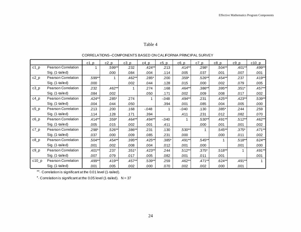
principals in the 37 schools. Table 4 shows the correlation coefficients among the Ten
Components themselves (and in this case all 10 are in fact present), while Table 5 again
shows how each of them are correlated with the three performance measures.
The intercorrelations among the Ten Components, based on the principals’ data, are
at least as great as those based on the teachers’ data, with the exception of C5 (Increased
and Effective Use of Instructional Time) (which was not present for teachers)12
. The
correlation between the components and the student performance measures are
comparable but slightly different from those presented for teachers in Table 3. Using the
principals’ data, Components 1 (Sound Administrative Practices), 2 (Aligned
Curriculum), 6 (Teacher Knowledge of Mathematics Content), and 7 (Instructional
Materials and Teaching Techniques) are significantly correlated with all of the
performance measures (as seen in Table 5).
A third set of measures for each component was obtained by averaging the separate
component values that were derived from teacher and principal data. This would be, in a
sense, the most complete school measure for each component. The intercorrelation
among this set of correlation coefficients are presented in Table 6, with their correlations
to the student performance measures shown in Table 7. In the case of C5 (Increased and
Effective Use of Instructional Time), the value based on the principal data was used, as
there was no value for C5 based on teacher data with which to average it. Using these
estimates of component values, all except C5 are significantly correlated with at least 8 of
the others, while Components 7, 8 (Differentiated Instruction), 9 (Focused Professional
Development) and 10 (End-of-Year Analysis) are significantly correlated with each of
the remaining 9, including C5.
The correlations of these last estimates of the Ten Components with the student
performance measures are similar to the previous set. As shown in Table 7, Components
1, 2, 7, 9 and 10 are significantly correlated with all four of the measures. C4 (Immediate
Intervention) is significantly correlated with proficiency at the Basic level and C6
(Teacher Knowledge of Mathematics Content) at the Below Basic level.
Effective Mathematics Program Components
24
Table 4
CORRELATIONS--COMPONENTS BASED ON CALIFORNIA PRINCIPAL SURVEY
1 .599** .232 .424** .213 .414** .298* .504** .401** .499**
.000 .084 .004 .114 .005 .037 .001 .007 .001
.599** 1 .462** .285* .200 .359* .526** .454** .237 .419**
.000 .002 .044 .128 .015 .000 .002 .079 .005
.232 .462** 1 .274 .168 .464** .386** .395** .351* .457**
.084 .002 .050 .171 .002 .009 .008 .017 .002
.424** .285* .274 1 -.048 .494** .231 .425** .423** .539**
.004 .044 .050 .394 .001 .085 .004 .005 .000
.213 .200 .168 -.048 1 -.040 .130 .385* .244 .259
.114 .128 .171 .394 .411 .231 .012 .082 .070
.414** .359* .464** .494** -.040 1 .530** .491** .512** .462**
.005 .015 .002 .001 .411 .000 .001 .001 .002
.298* .526** .386** .231 .130 .530** 1 .545** .375* .471**
.037 .000 .009 .085 .231 .000 .000 .011 .002
.504** .454** .395** .425** .385* .491** .545** 1 .518** .624**
.001 .002 .008 .004 .012 .001 .000 .001 .000
.401** .237 .351* .423** .244 .512** .375* .518** 1 .491**
.007 .079 .017 .005 .082 .001 .011 .001 .001
.499** .419** .457** .539** .259 .462** .471** .624** .491** 1
.001 .005 .002 .000 .070 .002 .002 .000 .001
Pearson Correlation
Sig. (1-tai led)
Pearson Correlation
Sig. (1-tai led)
Pearson Correlation
Sig. (1-tai led)
Pearson Correlation
Sig. (1-tai led)
Pearson Correlation
Sig. (1-tai led)
Pearson Correlation
Sig. (1-tai led)
Pearson Correlation
Sig. (1-tai led)
Pearson Correlation
Sig. (1-tai led)
Pearson Correlation
Sig. (1-tai led)
Pearson Correlation
Sig. (1-tai led)
c1_p
c2_p
c3_p
c4_p
c5_p
c6_p
c7_p
c8_p
c9_p
c10_p
c1_p c2_p c3_p c4_p c5_p c6_p c7_p c8_p c9_p c10_p
Correlation is significant at the 0.01 level (1-tai led).**.
Correlation is significant at the 0.05 level (1-tai led). N = 37*.

Effective Mathematics Program Components
25
Table 5
CORRELATIONS--CALIFORNIA PRINCIPAL-BASED COMPONENTS WITH
STUDENT PERFORMANCE MEASURES
.399** .394** .404** .385**
.007 .008 .007 .009
.382** .510** .534** .530**
.010 .001 .000 .000
.040 .092 .075 .072
.407 .294 .329 .336
.049 .047 -.009 .024
.387 .391 .479 .443
.117 .091 .086 .105
.256 .305 .314 .277
.421** .366* .353* .347*
.005 .013 .016 .018
.502** .517** .491** .525**
.001 .001 .001 .000
.157 .168 .183 .146
.177 .160 .139 .194
.262 .242 .227 .223
.059 .075 .088 .092
.212 .208 .172 .193
.104 .109 .154 .126
1 .880** .823** .866**
.000 .000 .000
.880** 1 .968** .988**
.000 .000 .000
.823** .968** 1 .968**
.000 .000 .000
.866** .988** .968** 1
.000 .000 .000
Pearson Correlation
Sig. (1-tailed)
Pearson Correlation
Sig. (1-tailed)
Pearson Correlation
Sig. (1-tailed)
Pearson Correlation
Sig. (1-tailed)
Pearson Correlation
Sig. (1-tailed)
Pearson Correlation
Sig. (1-tailed)
Pearson Correlation
Sig. (1-tailed)
Pearson Correlation
Sig. (1-tailed)
Pearson Correlation
Sig. (1-tailed)
Pearson Correlation
Sig. (1-tailed)
Pearson Correlation
Sig. (1-tailed)
Pearson Correlation
Sig. (1-tailed)
Pearson Correlation
Sig. (1-tailed)
Pearson Correlation
Sig. (1-tailed)
c1_p
c2_p
c3_p
c4_p
c5_p
c6_p
c7_p
c8_p
c9_p
c10_p
ppm_bb
ppm_b
ppm_p
pctl_b
ppm_bb ppm_b ppm_p pctl_b
Correlation is significant at the 0.01 level (1-tailed).**.
Correlation is significant at the 0.05 level (1-tailed).
N = 37 except c5_p = 34
*.

Effective Mathematics Program Components
26
Table 6
CORRELATIONS--COMPONENTS BASED ON CALIFORNIA TEACHER AND PRINCIPAL SURVEYS
1 .715** .419** .587** .280 .425** .504** .526** .465** .510**
.000 .005 .000 .055 .004 .001 .000 .002 .001
.715** 1 .511** .497** .270 .492** .691** .430** .408** .444**
.000 .001 .001 .062 .001 .000 .004 .006 .003
.419** .511** 1 .340* .208 .387** .437** .418** .415** .472**
.005 .001 .020 .118 .009 .003 .005 .005 .002
.587** .497** .340* 1 -.003 .582** .340* .500** .533** .577**
.000 .001 .020 .493 .000 .020 .001 .000 .000
.280 .270 .208 -.003 1 .012 .309* .469** .319* .295*
.055 .062 .118 .493 .473 .038 .003 .033 .045
.425** .492** .387** .582** .012 1 .537** .415** .514** .457**
.004 .001 .009 .000 .473 .000 .005 .001 .002
.504** .691** .437** .340* .309* .537** 1 .505** .372* .605**
.001 .000 .003 .020 .038 .000 .001 .012 .000
.526** .430** .418** .500** .469** .415** .505** 1 .561** .553**
.000 .004 .005 .001 .003 .005 .001 .000 .000
.465** .408** .415** .533** .319* .514** .372* .561** 1 .531**
.002 .006 .005 .000 .033 .001 .012 .000 .000
.510** .444** .472** .577** .295* .457** .605** .553** .531** 1
.001 .003 .002 .000 .045 .002 .000 .000 .000
Pearson Correlation
Sig. (1-tailed)
Pearson Correlation
Sig. (1-tailed)
Pearson Correlation
Sig. (1-tailed)
Pearson Correlation
Sig. (1-tailed)
Pearson Correlation
Sig. (1-tailed)
Pearson Correlation
Sig. (1-tailed)
Pearson Correlation
Sig. (1-tailed)
Pearson Correlation
Sig. (1-tailed)
Pearson Correlation
Sig. (1-tailed)
Pearson Correlation
Sig. (1-tailed)
c1_tp
c2_tp
c3_tp
c4_tp
c5_tp
c6_tp
c7_tp
c8_tp
c9_tp
c10_tp
c1_tp c2_tp c3_tp c4_tp c5_tp c6_tp c7_tp c8_tp c9_tp c10_tp
Correlation is significant at the 0.01 level (1-tai led).**.
Correlation is significant at the 0.05 level (1-tai led). N = 37*.

Effective Mathematics Program Components
27
Table 7
CORRELATIONS--COMPONENTS BASED ON CALIFORNIA TEACHER AND
PRINCIPAL SURVEYS WITH STUDENT PERFORMANCE MEASURES
.497** .596** .628** .589**
.001 .000 .000 .000
.424** .517** .547** .534**
.004 .001 .000 .000
.116 .164 .168 .121
.248 .166 .161 .238
.196 .277* .269 .255
.123 .048 .054 .064
.117 .091 .086 .105
.256 .305 .314 .277
.300* .258 .244 .248
.036 .062 .073 .069
.552** .579** .586** .583**
.000 .000 .000 .000
.131 .165 .201 .135
.221 .164 .116 .212
.289* .302* .302* .283*
.041 .035 .035 .045
.334* .386** .357* .357*
.022 .009 .015 .015
1 .880** .823** .866**
.000 .000 .000
.880** 1 .968** .988**
.000 .000 .000
.823** .968** 1 .968**
.000 .000 .000
.866** .988** .968** 1
.000 .000 .000
Pearson Correlation
Sig. (1-tailed)
Pearson Correlation
Sig. (1-tailed)
Pearson Correlation
Sig. (1-tailed)
Pearson Correlation
Sig. (1-tailed)
Pearson Correlation
Sig. (1-tailed)
Pearson Correlation
Sig. (1-tailed)
Pearson Correlation
Sig. (1-tailed)
Pearson Correlation
Sig. (1-tailed)
Pearson Correlation
Sig. (1-tailed)
Pearson Correlation
Sig. (1-tailed)
Pearson Correlation
Sig. (1-tailed)
Pearson Correlation
Sig. (1-tailed)
Pearson Correlation
Sig. (1-tailed)
Pearson Correlation
Sig. (1-tailed)
c1_tp
c2_tp
c3_tp
c4_tp
c5_tp
c6_tp
c7_tp
c8_tp
c9_tp
c10_tp
ppm_bb
ppm_b
ppm_p
pctl_b
ppm_bb ppm_b ppm_p pctl_b
Correlation is significant at the 0.01 level (1-tailed).**.
Correlation is significant at the 0.05 level (1-tailed).
N = 37, ecept for c5_to B = 34
*.
A summary of some of the correlation coefficients introduced above is contained in
Table 8. Column 1 shows those for each component derived from teachers’ data with
student performance using the Basic criterion. Column 2 shows the corresponding
correlation coefficients based on principals’ data, and column 4 shows the correlation
coefficients corresponding to each component based on the averages of teacher and
principal responses. These numbers appeared separately in Tables 3, 5, and 7 above.

Effective Mathematics Program Components
28
Table 8
Summary, Correlation Coefficients Between Ten Components and Student Performance
Measure and Between Teacher and Principal Component Measures--California
Component
Cor. Coef.
Btwn Teacher
Components
and Student
Performance
(PPM_B)
(Sig.)
(Col 1)
Cor. Coef.
Btwn Principal
Components
and Student
Performance
(PPM_B)
(Sig)
(Col 2)
Cor. Coef.
Btwn Teacher
and Principal
Components
(Sig)
(Col 3)
Cor. Coef.
Btwn Teacher-
Principal
Components
and Student
Performance
(PPM_B)
(Sig)
(Col 4)
1 .576**
.000
.394*
.008
.268
.055
.596**
.000
2 .267
.055
.510**
.001
.312*
.030
.517**
.001
3 .224
.091
.092
.294
.314*
.030
.164
.166
4 .400**
.007
.047
.391
.459**
.002
.277*
.048
5 --
.091
.305 --
.091
.305
6 -.031
.428
.366*
.013
.460**
.002
.258
.062
7 .388**
.009
.517**
.001
.251
.067
.579**
.000
8 .080
.320
.168
.160
.357*
.015
.165
.164
9 .301*
.035
.242
.075
.462**
.002
.302*
.035
10 .452**
.003
.208
.109
.017
.461
.386*
.009 ** Correlation is significant at the .01 level (1-tailed)
* Correlation is significant at the .05 level (1-tailed)
Column 3 contains new information. The numbers in this column are the correlation
coefficients calculated with teachers’ responses (averaged) to each component as one of
the variables, and the responses of principals to each component as the other variable. In
short, high values (close to 1) in column 3 would represent a very high degree of
consistency between teachers’ assessments of the degree of implementation of the Ten
Components and those of the principals at their respective schools. As seen, the

Effective Mathematics Program Components
29
correlations for 6 of the components are statistically significant. For two others—C1
(Sound Administrative Practices) and C7 (Instructional Materials and Teaching
Techniques) -- the significance values are 0.055 and 0.067. C10 (End-of-Year Analysis)
is far from significant with a value of 0.461. Given that the numbers of teachers’
questionnaires averaged just under 10 per school, while there was just a single principal’s
questionnaire for each school, these results seem reasonably indicative of within-school
coherence of attitudes among teachers and principals, although a greater degree of
correlation would have been desirable.
Having established a certain degree of consistency among the various measures for
each component, and having demonstrated that a percentile rank of student performance
can be substituted for the percentage of students tested who achieve the Basic level of
competence, these data will now be used in attempting to explain the variation in school
and school district performance.
Ordinary least-squares regression was used to determine how well the estimated
component values explain variation in student performance at the campus level. The
independent variables used will be the component values described above, calculated as
the simple averages of those based upon teachers’ and principals’ data. In addition, in the
first regression the variable named FRL will also be included as an independent variable.
FRL represents the percentage of economically disadvantaged students at a campus, as
determined by their eligibility for the federal free or reduced-price lunch program. The
dependent variable used was PCTL_B, the percentile rank for each school based on
passing the mathematics portion of the California Standards Test, using the Basic
criterion as the level of performance. The resulting table of coefficients is shown in
Table 9.
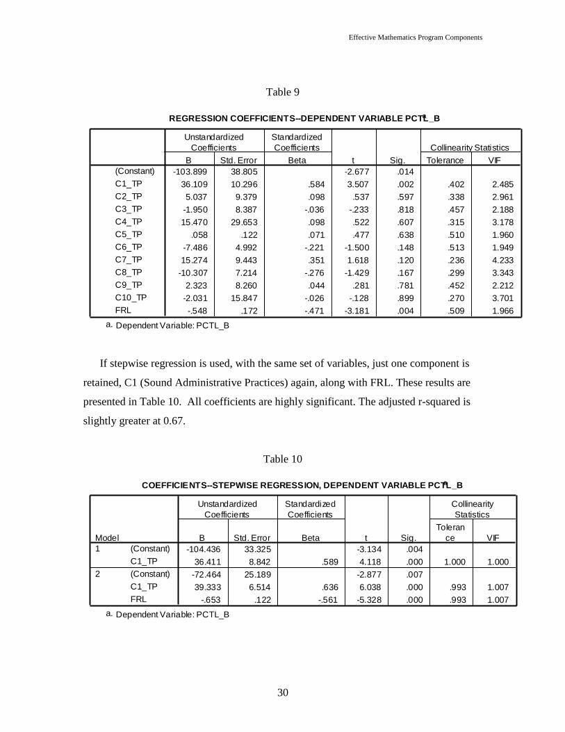
Due to several instances of missing data, the total number of observations was just 33.
Trying to estimate 11 coefficients plus the intercept with 33 observations is a stretch.
Two of the slope coefficients were significant, those for C1 (Sound Administrative
Practices) and FRL. The adjusted R-squared was 0.632. The collinearity statistic—
VIF—never approaches the conservative recommended value of 10. This indicates that
although there is a fair degree of intercorrelation among the Ten Components, as
discussed above, they do not appear to be linearly dependent.
Effective Mathematics Program Components
30
Table 9
REGRESSION COEFFICIENTS--DEPENDENT VARIABLE PCTL_Ba
-103.899 38.805 -2.677 .014
36.109 10.296 .584 3.507 .002 .402 2.485
5.037 9.379 .098 .537 .597 .338 2.961
-1.950 8.387 -.036 -.233 .818 .457 2.188
15.470 29.653 .098 .522 .607 .315 3.178
.058 .122 .071 .477 .638 .510 1.960
-7.486 4.992 -.221 -1.500 .148 .513 1.949
15.274 9.443 .351 1.618 .120 .236 4.233
-10.307 7.214 -.276 -1.429 .167 .299 3.343
2.323 8.260 .044 .281 .781 .452 2.212
-2.031 15.847 -.026 -.128 .899 .270 3.701
-.548 .172 -.471 -3.181 .004 .509 1.966
(Constant)
C1_TP
C2_TP
C3_TP
C4_TP
C5_TP
C6_TP
C7_TP
C8_TP
C9_TP
C10_TP
FRL
B Std. Error
Unstandardized
Coefficients
Beta
Standardized
Coefficients
t Sig. Tolerance VIF
Collinearity Statistics
Dependent Variable: PCTL_Ba.
If stepwise regression is used, with the same set of variables, just one component is
retained, C1 (Sound Administrative Practices) again, along with FRL. These results are
presented in Table 10. All coefficients are highly significant. The adjusted r-squared is
slightly greater at 0.67.
Table 10
COEFFICIENTS--STEPWISE REGRESSION, DEPENDENT VARIABLE PCTL_Ba
-104.436 33.325 -3.134 .004
36.411 8.842 .589 4.118 .000 1.000 1.000
-72.464 25.189 -2.877 .007
39.333 6.514 .636 6.038 .000 .993 1.007
-.653 .122 -.561 -5.328 .000 .993 1.007
(Constant)
C1_TP
(Constant)
C1_TP
FRL
Model
1
2
B Std. Error
Unstandardized
Coefficients
Beta
Standardized
Coefficients
t Sig.
Toleran
ce VIF
Collinearity
Statistics
Dependent Variable: PCTL_Ba.

Effective Mathematics Program Components
31
A third regression was performed, again stepwise, but two additional variables were
put into the pool—NOT_HSG, an estimate of the percentage of parents who are not high
school graduates, and SMOB, a measure of the degree of campus mobility (students who
change schools during the academic year).13
Both of these additional variables were
retained by the stepwise procedure, and FRL as well as C1 (Sound Administrative
Practices) were still included also. The adjusted r-squared increased to 0.72. If C1 is
deliberately removed from the regression, and then reinserted, the adjusted r-squared
improves from 0.30, without it, to the 0.72 with it. It thus appears that the differing
quality of school administration, measured by responses to the items within this
component, account for a remarkable 40 percent of the intercampus variation in student
performance at the school level, as measured by the Basic criterion.
The final stage in the analysis of the California survey data will be to use HLM to
determine how the remaining unexplained variance is split between the campus level and
the district level.
Application of Hierarchical Linear Model (HLM) Analysis to California Data
Although constrained by having just seven school districts for which the survey data
are available, HLM was used to attempt to determine if an appreciable amount of the
observed campus variance in student performance might be due to variations at the
district level, as distinct from the campus level, and, if possible, to explain any such inter-
district variance. In the following discussion, it should be kept in mind that HLM analysis
depends crucially upon the recognition that entities are grouped together. In the present
case, several schools are grouped within each of the school districts. Separate school
level (level 1) and district level (level 2) data sets are constructed which reflect this
feature of the school system, and which are utilized by the HLM computer software in
distinguishing effects at each level.
The steps followed can best be described within the context of a series of equation
sets that represent the models fitted by the HLM analysis at increasing degrees of
complexity, i.e., as additional terms and equations are added. The equations are
distinguished as being either those pertaining to level 1 (schools) or level 2 (school
districts).

Effective Mathematics Program Components
32
Table 11 shows the results for a sequence of 5 different models. The first, Model 1, is
really not a model at all, but can be cast into the HLM equation framework. That is,
equation 1(a) indicates that the dependent variable, PCTL_B, is being ―predicted‖ by B0j
plus an error term, rij. As a reminder, recall that subscript i refers to a school within the
district j. Equation 1(b), the level 2 equation in HLM parlance, merely asserts that B0j of
equation 1(a) is made up only of a constant, namely g00. In effect, then, the HLM
program, in this case, in determining a value for the constant B0j, is calculating the mean
of PCTL_Bij for all schools and all districts in the sample. The variance of the random
term rij is the same as the variance of PCTL_B, and is shown to be 526.6. This, then, is
the total variance of the school-based test scores, which were expressed in percentile
terms (with PCTL_B being used as the dependent variable, rather than PPM itself).
The equations for Model 2 of Table 11 differ from those for Model 1 only by the
addition of a random term, u0j, to equation 2(b). This is a crucial difference, however, for
it is this term that captures the extent to which the intercept of equation 2(a), B0j, differs
among the 7 districts. Note the variance is now divided between schools (level 1) and
school districts (level 2). Note also that all variance is still ―unexplained‖, in that no
independent variables have yet been introduced at either level. The unexplained variance
at the school level is shown to be 418.7, and that at the district level is 123.7, hence, 22.8
percent of the total unexplained variation in passing rates, measured in percentile terms,
is accounted for by district level phenomena.

Effective Mathematics Program Components
33
Table 11
Hierarchical Linear Model Results, California
HLM Equations
Significance
(p-values)
Unexplained
Variance
Level 2
Pct
Variance
Deg. of
Freedom
FRL Cj Lev.
1
Lev.
2
Lev.
1
Lev.
2
Model 1
Level 1
(a) PCTL_B = B0j + rij
Level 2
(b) B0j = g00
526.6
36
Model 2
Level 1
(a) PCTL_B = B0j + rij
Level 2
(b) B0j = g00 + u0j
418.7
123.7
22.8%
36
6
Model 3
Level 1
(a) PCTL_B = B0j +B1FRLij+ rij
Level 2
(b) B0j = g00 + u0j
(c) B1 = g10
.002
309.7
121.7
28.2%
35
6
Model 4
Level 1
(a) PCTL_B = B0j +B1FRLij+ rij
Level 2
(b) B0j = g00 + g01C1_DISTj + u0j
(c) B1 = g10
.002
.596
310.2
146.4
32.1%
34
5
Model 5
Level 1
(a) PCTL_B = B0j +B1FRLij+ rij
Level 2
(b) B0j = g00 + g01C1_TPAj + u0j
(c) B1 = g10
.000
.017
298.4
0.3
0.0%
34
5

Effective Mathematics Program Components
34
The effects of introducing the percentage of students in each school who are
economically disadvantaged (FRL) is shown in Model 3 in Table 11. Note that a term
including FRL has been added to equation 3(a). This results in another level 2 equation,
3(c), showing that B1 is represented by the constant (slope) coefficient, g10. Represented
in this way, this slope coefficient for FRL is assumed to be the same for all schools in all
districts.
The introduction of FRL at level 1 has now accounted for some of the variance of
PCTL_B, with the amount of unexplained variance attributed to level 1 now at 309.7, and
that at level 2 at 121.7. The unexplained variance at level 2 is now 28.2 percent of the
total remaining unexplained variance. The t-value for the slope coefficient of FRL, B1, is
statistically significant, having a p-value of 0.002. Note also that although the
introduction of FRL in the level 1 equation reduced level 1 unexplained variance from
418.7 to 309.7; the level 2 unexplained interdistrict variance decreased only slightly,
from 123.7 to 121.7. When expressed as a percentage of remaining unexplained variance,
however, it increased from 22.8 percent to 28.2 percent.
The next step involves introducing one of the district level components to try to
account for some of the unexplained variation between districts. The results of the first
attempt are presented in Table 11 as Model 4. The new variable in equation 4(b),
designated as C1_DIST, was derived by averaging the responses of the district
administration to the items in C1 (Sound Administrative Practices). As can be seen, the
inclusion of this level 2 variable did not explain any of the interdistrict variance. In fact,
due to the reduction in the degrees of freedom from 6 to 5, the estimated unexplained
variance actually increased, from 121.7 to 146.4. Nor is the estimated coefficient
associated with C1_DIST significant, having a p-value of just 0.596.
These results were disappointing. As an alternative, component values for the district
level were calculated by averaging the component values for schools, by district.
Substituting the values so derived for the first component, designated C1_TPA, into
equation 5(b) (Model 5, Table 11) results in a considerable improvement. The level 1
unexplained variance remains essentially unchanged, as expected, but level 2 unexplained
variance decreased from 121.7 using Model 3 to only 0.3 with Model 5, somewhat
astonishingly.

Effective Mathematics Program Components
35
Figure 5
District Performance Measures v Component 1
This last result obviously suggests a high degree of correlation between the average
values of C1_TPA and the measures of district performance. In the current case, the
measure of each district’s performance is precisely the values established for uoj in Model
3, which we have referred to as ―modified mean residuals‖ (MMRs). A scatterplot of
these MMRs plotted against the values of C1_TPA, as used in Model 5, is shown in
Figure 5. The association between the two variables is inescapable.

Effective Mathematics Program Components
36
Table 12
COMPARISON OF CORRELATIONS BETWEEN CALIFORNIA DISTRICT
PERFORMANCE MEASURE (MMR) AND TWO DIFFERENT SETS OF DISTRICT
LEVEL COMPONENT VALUES
.889** .000
.004 .500
.951** .689*
.000 .044
.675* .147
.048 .377
.744* .206
.028 .329
.259 .215
.288 .322
.732* -.300
.031 .257
.906** -.495
.002 .129
.170 .117
.358 .401
.152 -.651
.373 .057
.914** .071
.002 .440
Sig. (1-tailed)
Sig. (1-tailed)
Sig. (1-tailed)
Sig. (1-tailed)
Sig. (1-tailed)
Sig. (1-tailed)
Sig. (1-tailed)
Sig. (1-tailed)
Sig. (1-tailed)
Sig. (1-tailed)
c1
c2
c3
c4
c5
c6
c7
c8
c9
c10
DISTRICT
COMPONENTS,
BASED ON
TEACHER AND
PRINCIPAL
SURVEYS
(Col 1)
DISTRICT
COMPONENTS,
BASED ON
DISTRICT
LEVEL
SURVEYS
(Col 2)
Correlation is significant at the 0.01 level (1-tailed).**.
Correlation is significant at the 0.05 level (1-tailed). N = 7*.
The differences in alignment between the other district components, when determined
using the two different methods as described above, was explored using their correlations
with the district performance measures, MMRs, for each component. These correlation
components are presented in Table 12. In column 2 the estimates of component values
based only on the district level surveys are presented, while column 1 shows those that
relied upon the district level components which came from averaging the teacher and
principal survey results to the district level. It is obvious why C1_TPA is so much more
effective in explaining variance in PCTL_M than is C1_DIST. The correlation between

Effective Mathematics Program Components
37
MMR and C1_TPA for the 7 districts is 0.889, while that for C1_DIST is exactly 0.0,
signifying absolutely no correlation between MMR and C1_DIST.
The highly significant correlation coefficients in column 1 for C2 (Aligned
Curriculum), is even greater than that for C1 (Sound Administrative Practices), which
was used in Model 5 (see Table 11). And those for C7 (Instructional Materials and
Teaching Techniques) and C10 (End-of-Year Analysis) are also greater. In addition, the
significance levels for C3 (Ongoing Assessment), C4 (Immediate Intervention) and C6
(Teacher Knowledge of Mathematics Content) are beneath the 0.05 level, at 0.048, 0.028
and 0.031, respectively. In contrast, none of the correlation coefficients in column 2
except C2 are statistically significant. A scatterplot matrix is shown in Figure 6. The
variables MMR_M3, C1, C2, C7, and C10 are all plotted against one another in pairs.
The top row shows MMR_M3 on the vertical axis and the various components on the
horizontal axis in each of the 4 diagrams. The suffix ―M3‖ is added to MMR to indicated
that these are the district performance measures obtained from Model 3, as represented in
Table 11. As a reminder, this model estimated how much unexplained variance could be
attributed to level 1 (schools) and how much to level 2 (districts) after adjusting for the
proportions of economically disadvantaged students in each school.
The patterns of association between MMR_M3 and each of the four components
shown in Figure 6 are compelling and consistent. This suggests that all of the district
practices represented by these components are likely candidates for policies to improve
school performance through district influences. Districts with the highest marks on these
components are those whose schools, on average, do better than predicted, in comparison
with schools in the districts with the lowest marks for these four components, as recorded
by teachers and principals included in the survey.

Effective Mathematics Program Components
38
Figure 6
District Performance Measure (MMR_M3) Plotted
Against Four District Level Components
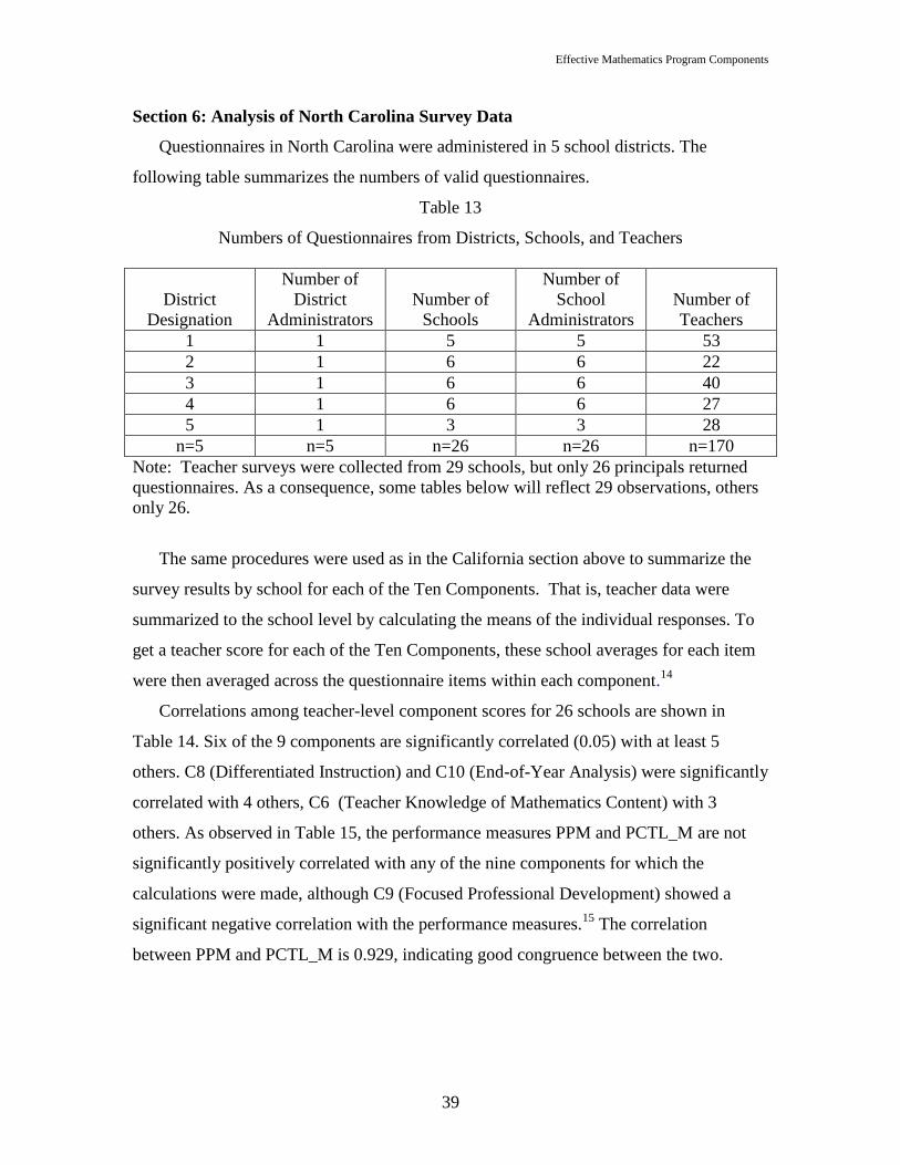
Effective Mathematics Program Components
39
Section 6: Analysis of North Carolina Survey Data
Questionnaires in North Carolina were administered in 5 school districts. The
following table summarizes the numbers of valid questionnaires.
Table 13
Numbers of Questionnaires from Districts, Schools, and Teachers
District
Designation
Number of
District
Administrators
Number of
Schools
Number of
School
Administrators
Number of
Teachers
1 1 5 5 53
2 1 6 6 22
3 1 6 6 40
4 1 6 6 27
5 1 3 3 28
n=5 n=5 n=26 n=26 n=170
Note: Teacher surveys were collected from 29 schools, but only 26 principals returned
questionnaires. As a consequence, some tables below will reflect 29 observations, others
only 26.
The same procedures were used as in the California section above to summarize the
survey results by school for each of the Ten Components. That is, teacher data were
summarized to the school level by calculating the means of the individual responses. To
get a teacher score for each of the Ten Components, these school averages for each item
were then averaged across the questionnaire items within each component.14
Correlations among teacher-level component scores for 26 schools are shown in
Table 14. Six of the 9 components are significantly correlated (0.05) with at least 5
others. C8 (Differentiated Instruction) and C10 (End-of-Year Analysis) were significantly
correlated with 4 others, C6 (Teacher Knowledge of Mathematics Content) with 3
others. As observed in Table 15, the performance measures PPM and PCTL_M are not
significantly positively correlated with any of the nine components for which the
calculations were made, although C9 (Focused Professional Development) showed a
significant negative correlation with the performance measures.15
The correlation
between PPM and PCTL_M is 0.929, indicating good congruence between the two.

Effective Mathematics Program Components
40
Table 14
CORRELATIONS-- COMPONENTS BASED ON NORTH CAROLINA TEACHER SURVEYS
1 .480** .295 .414* .461** .435** .043 .654** .083
.004 .060 .013 .006 .009 .412 .000 .334
.480** 1 .628** .625** .368* .425* .456** .396* .299
.004 .000 .000 .025 .011 .006 .017 .058
.295 .628** 1 .811** .149 .429* .687** .358* .474**
.060 .000 .000 .220 .010 .000 .028 .005
.414* .625** .811** 1 .221 .476** .685** .445** .345*
.013 .000 .000 .125 .005 .000 .008 .033
.461** .368* .149 .221 1 .290 -.013 .581** .144
.006 .025 .220 .125 .063 .474 .000 .229
.435** .425* .429* .476** .290 1 .039 .534** .236
.009 .011 .010 .005 .063 .420 .001 .108
.043 .456** .687** .685** -.013 .039 1 .175 .331*
.412 .006 .000 .000 .474 .420 .182 .040
.654** .396* .358* .445** .581** .534** .175 1 .349*
.000 .017 .028 .008 .000 .001 .182 .032
.083 .299 .474** .345* .144 .236 .331* .349* 1
.334 .058 .005 .033 .229 .108 .040 .032
Pearson Correlation
Sig. (1-tailed)
Pearson Correlation
Sig. (1-tailed)
Pearson Correlation
Sig. (1-tailed)
Pearson Correlation
Sig. (1-tailed)
Pearson Correlation
Sig. (1-tailed)
Pearson Correlation
Sig. (1-tailed)
Pearson Correlation
Sig. (1-tailed)
Pearson Correlation
Sig. (1-tailed)
Pearson Correlation
Sig. (1-tailed)
c1_t
c2_t
c3_t
c4_t
c6_t
c7_t
c8_t
c9_t
c10_t
c1_t c2_t c3_t c4_t c6_t c7_t c8_t c9_t c10_t
Correlation is significant at the 0.01 level (1-tailed).**.
Correlation is significant at the 0.05 level (1-tailed). N = 29*.

Effective Mathematics Program Components
41
Table 15
CORRELATIONS--TEACHER-BASED COMPONENTS WITH
STUDENT PERFORMANCE MEASURES, NORTH CAROLINA
.052 .126
.394 .257
.221 .186
.125 .166
.020 .083
.458 .335
.005 .092
.490 .317
-.030 -.035
.438 .429
.069 .152
.362 .215
-.050 -.054
.399 .391
-.355* -.345*
.029 .033
-.160 -.273
.204 .076
1 .929**
.000
.929** 1
.000
Pearson Correlation
Sig. (1-tailed)
Pearson Correlation
Sig. (1-tailed)
Pearson Correlation
Sig. (1-tailed)
Pearson Correlation
Sig. (1-tailed)
Pearson Correlation
Sig. (1-tailed)
Pearson Correlation
Sig. (1-tailed)
Pearson Correlation
Sig. (1-tailed)
Pearson Correlation
Sig. (1-tailed)
Pearson Correlation
Sig. (1-tailed)
Pearson Correlation
Sig. (1-tailed)
Pearson Correlation
Sig. (1-tailed)
c1_t
c2_t
c3_t
c4_t
c6_t
c7_t
c8_t
c9_t
c10_t
ppm
pctl_m
ppm pctl_m
Correlation is significant at the 0.01 level (1-tailed).**.
Correlation is significant at the 0.05 level (1-tailed).
N = 29
*.
Similar correlation coefficients were calculated based upon data collected from the
principals in 26 schools. Table 16 shows the correlation coefficients among the Ten
Components themselves (and in this case all 10 are in fact present), while Table 17 again
shows how each of them is correlated with the performance measures.

Effective Mathematics Program Components
42
Table 16
CORRELATIONS--COMPONENTS BASED ON PRINCIPAL SURVEY, NORTH CAROLINA
1 .068 .215 .331* -.012 .067 .308 .235 -.051 -.092
.371 .145 .049 .476 .372 .063 .124 .403 .328
.068 1 .082 -.268 -.088 -.145 .036 -.067 .148 -.033
.371 .346 .093 .335 .240 .430 .373 .235 .437
.215 .082 1 .202 .067 .312 .374* .230 .455** .244
.145 .346 .161 .372 .060 .030 .129 .010 .115
.331* -.268 .202 1 .375* .141 -.041 .346* .107 .319
.049 .093 .161 .030 .247 .421 .042 .302 .056
-.012 -.088 .067 .375* 1 -.021 .141 -.041 -.115 .170
.476 .335 .372 .030 .459 .246 .420 .287 .203
.067 -.145 .312 .141 -.021 1 .547** .523** .593** .648**
.372 .240 .060 .247 .459 .002 .003 .001 .000
.308 .036 .374* -.041 .141 .547** 1 .207 .237 .161
.063 .430 .030 .421 .246 .002 .155 .122 .217
.235 -.067 .230 .346* -.041 .523** .207 1 .288 .472**
.124 .373 .129 .042 .420 .003 .155 .077 .007
-.051 .148 .455** .107 -.115 .593** .237 .288 1 .607**
.403 .235 .010 .302 .287 .001 .122 .077 .000
-.092 -.033 .244 .319 .170 .648** .161 .472** .607** 1
.328 .437 .115 .056 .203 .000 .217 .007 .000
Pearson Correlation
Sig. (1-tailed)
Pearson Correlation
Sig. (1-tailed)
Pearson Correlation
Sig. (1-tailed)
Pearson Correlation
Sig. (1-tailed)
Pearson Correlation
Sig. (1-tailed)
Pearson Correlation
Sig. (1-tailed)
Pearson Correlation
Sig. (1-tailed)
Pearson Correlation
Sig. (1-tailed)
Pearson Correlation
Sig. (1-tailed)
Pearson Correlation
Sig. (1-tailed)
c1_p
c2_p
c3_p
c4_p
c5_p
c6_p
c7_p
c8_p
c9_p
c10_p
c1_p c2_p c3_p c4_p c5_p c6_p c7_p c8_p c9_p c10_p
Correlation is significant at the 0.05 level (1-tai led).*.
Correlation is significant at the 0.01 level (1-tai led). N = 26**.

Effective Mathematics Program Components
43
Table 17
CORRELATIONS--PRINCIPAL-BASED COMPONENTS WITH
STUDENT PERFORMANCE MEASURES, NORTH CAROLINA
-.161 -.264
.216 .096
-.052 -.093
.401 .326
-.070 -.036
.366 .431
-.227 -.164
.133 .211
-.029 -.120
.444 .279
.103 .040
.308 .423
.141 .083
.246 .343
-.376* -.492**
.029 .005
.037 .060
.429 .386
.161 .111
.215 .294
1 .929**
.000
.929** 1
.000
Pearson Correlation
Sig. (1-tailed)
Pearson Correlation
Sig. (1-tailed)
Pearson Correlation
Sig. (1-tailed)
Pearson Correlation
Sig. (1-tailed)
Pearson Correlation
Sig. (1-tailed)
Pearson Correlation
Sig. (1-tailed)
Pearson Correlation
Sig. (1-tailed)
Pearson Correlation
Sig. (1-tailed)
Pearson Correlation
Sig. (1-tailed)
Pearson Correlation
Sig. (1-tailed)
Pearson Correlation
Sig. (1-tailed)
Pearson Correlation
Sig. (1-tailed)
c1_p
c2_p
c3_p
c4_p
c5_p
c6_p
c7_p
c8_p
c9_p
c10_p
ppm
pctl_m
ppm pctl_m
Correlation is significant at the 0.05 level (1-tailed).*.
Correlation is significant at the 0.01 level
(1-tailed). N = 26
**.

Effective Mathematics Program Components
44
Table 18
CORRELATIONS--TEACHER/PRINCIPAL AVERAGES OF COMPONENT VALUES, NORTH CAROLINA
1 .316* .437** .288 -.104 .294 .214 .379* .504** .219
.048 .009 .065 .306 .061 .133 .021 .003 .127
.316* 1 .165 .518** -.236 -.200 .132 .361* .051 .050
.048 .195 .002 .123 .149 .248 .027 .397 .398
.437** .165 1 .349* -.011 .181 .501** .434** .400* .209
.009 .195 .032 .480 .174 .003 .009 .016 .139
.288 .518** .349* 1 -.106 -.175 .233 .526** .168 .373*
.065 .002 .032 .304 .182 .112 .002 .191 .023
-.104 -.236 -.011 -.106 1 .027 .144 -.150 .059 .236
.306 .123 .480 .304 .448 .241 .233 .388 .123
.294 -.200 .181 -.175 .027 1 .414* .160 .545** .479**
.061 .149 .174 .182 .448 .013 .204 .001 .004
.214 .132 .501** .233 .144 .414* 1 .261 .321* .472**
.133 .248 .003 .112 .241 .013 .086 .045 .005
.379* .361* .434** .526** -.150 .160 .261 1 .230 .541**
.021 .027 .009 .002 .233 .204 .086 .115 .001
.504** .051 .400* .168 .059 .545** .321* .230 1 .441**
.003 .397 .016 .191 .388 .001 .045 .115 .008
.219 .050 .209 .373* .236 .479** .472** .541** .441** 1
.127 .398 .139 .023 .123 .004 .005 .001 .008
Pearson Correlation
Sig. (1-tailed)
Pearson Correlation
Sig. (1-tailed)
Pearson Correlation
Sig. (1-tailed)
Pearson Correlation
Sig. (1-tailed)
Pearson Correlation
Sig. (1-tailed)
Pearson Correlation
Sig. (1-tailed)
Pearson Correlation
Sig. (1-tailed)
Pearson Correlation
Sig. (1-tailed)
Pearson Correlation
Sig. (1-tailed)
Pearson Correlation
Sig. (1-tailed)
c1_ptavg
c2_ptavg
c3_ptavg
c4_ptavg
c5_ptavg
c6_ptavg
c7_ptavg
c8_ptavg
c9_ptavg
c10_
ptavg
c1_ptavg c2_ptavg c3_ptavg c4_ptavg c5_ptavg c6_ptavg c7_ptavg c8_ptavg c9_ptavg
c10_
ptavg
Correlation is significant at the 0.05 level (1-tailed).*.
Correlation is significant at the 0.01 level (1-tailed). N = 29**.

Effective Mathematics Program Components
45
Table 19
CORRELATIONS--COMPONENTS BASED ON TEACHER AND
PRINCIPAL SURVEYS WITH STUDENT PERFORMANCE
MEASURES, NORTH CAROLINA
-.035 -.070
.428 .359
.188 .102
.165 .300
-.026 .030
.447 .439
.181 .156
.173 .209
-.029 -.120
.444 .279
-.009 -.042
.481 .414
.176 .180
.180 .175
-.214 -.308
.132 .052
-.221 -.219
.124 .127
.093 -.013
.316 .473
1 .929**
.000
.929** 1
.000
Pearson Correlation
Sig. (1-tailed)
Pearson Correlation
Sig. (1-tailed)
Pearson Correlation
Sig. (1-tailed)
Pearson Correlation
Sig. (1-tailed)
Pearson Correlation
Sig. (1-tailed)
Pearson Correlation
Sig. (1-tailed)
Pearson Correlation
Sig. (1-tailed)
Pearson Correlation
Sig. (1-tailed)
Pearson Correlation
Sig. (1-tailed)
Pearson Correlation
Sig. (1-tailed)
Pearson Correlation
Sig. (1-tailed)
Pearson Correlation
Sig. (1-tailed)
c1_pt
c2_pt
c3_pt
c4_pt
c5_pt
c6_pt
c7_pt
c8_pt
c9_pt
c10_pt
ppm
pctl_m
ppm pctl_m
Correlation is significant at the 0.01 level (1-tailed).
N = 29
**.
There is considerably less interrcorrelaton among the Ten Components based on
principals’ responses to the survey than there was among teachers. For the principals,
(Table 16) only C6 (Teacher Knowledge of Mathematics Content) was significantly
correlated with as many as 4 other components, whereas in the case of teachers (Table
14) 6 of the components were correlated with at least 5 of the others. One of the
components in Table 16, C2, was not significantly correlated with any other component,
and C1 and C5 were significantly correlated with only one other.

Effective Mathematics Program Components
46
Referring to Table 17, there is only one instance of significant correlation between the
values for one of the components and the student performance measures, and this for C8
(Differentiated Instruction). Unfortunately, the correlation coefficients are negative (as
large as -0.492 when associated with the percentile-based measure), indicating that higher
ratings on Grouping for Instruction by principals is somewhat associated with lower
average student performance.
A third set of measures for each component was obtained by averaging the separate
component values which were derived from teacher and principal data. The results based
upon component values obtained by averaging those for teachers and principals are
presented in Tables 18 and 19. Using these estimates of component values, Table 18
shows that 4 of the components are significantly correlated with at least 5 others, 3 are
significantly correlated with 4 others, and C5 (Increased and Effective Use of
Instructional Time) is not significantly correlated with any of the other components. In
Table 19 it is observed that in no case is one of the components derived by averaging
those based on both teacher and principal survey data significantly correlated with a
measure of student performance.
The results presented in Tables 14 – 19 lead to the conclusion that teacher and
principals’ responses to the survey items are considerably less regular than were those
from the California surveys (Tables 2 – 7 above).16
Following the earlier discussion for California’s survey results, ordinary least-squares
regression was used to determine how well the estimated component values explain
variation in student performance at the campus level. The independent variables used
will be the component values described above, calculated as the simple averages of those
based upon teachers’ data and principals’ data. In addition, in the first regression the
variable named FRL was included as an independent variable. FRL represents the
percentage of economically disadvantaged students at a campus, as determined by their
eligibility for the federal free or reduced-price lunch program. The dependent variable
used was PCTL_M, the percentile rank for each school based on achieving Level III on
North Carolina’s end-of-course math test, in the elementary and middle-school grade
levels.

Effective Mathematics Program Components
47
When all 10 components plus FRL were used in a regression equation none of the
coefficients was significant. When the stepwise procedure was used only FRL was
retained, with a coefficient value of –0.553 (t-value = –3.247, p = 0.003). The adjusted r-
square was 0.276.
All-in-all, the results of the campus level analysis, using the survey data as described,
appears unimpressive. It remains to be seen if these data help explain any of the
interdistrict variation that might be present. For that analysis, the HLM framework will
again be used.
Hierarchical Linear Model (HLM) Analysis of North Carolina Data
Data from just 5 school districts were obtained in North Carolina. Consequently, the
analysis is even more tenuous than was that for California earlier (above), where there
were data for 7 school districts. The same sequence of HLM models was fitted for the
North Carolina data as was carried out earlier for California. The results for California
were summarized in Table 11. Those for North Carolina are presented in Table 20. Once
again, Model 1 is forced into the HLM framework, but is in actuality merely the ordinary
calculation of the variance of the dependent variable, PCTL_M. This variance, expressed
as the variance of the random term rij about the mean of PCTL_M, is 381.3. The
equations for Model 2 of Table 20 differ from those for Model 1 only by the addition of a
random term, u0j, to equation 2(b). As explained earlier, however, this is a crucial
difference, for it is this term that captures the extent to which the intercept of equation
2(a), B0j, differs among the 5 districts. The variance is now divided between schools
(level 1) and school districts (level 2). All variance is still ―unexplained‖, in that no
independent variables have yet been introduced at either level. The unexplained variance
at the school level is shown to be 325.9, and that at the district level is 65.8. Therefore,
16.8 percent of the total unexplained variation in passing rates, measured in percentile
terms, is accounted for by district level phenomena.

Effective Mathematics Program Components
48
Table 20
Hierarchical Linear Model Results, North Carolina
HLM Equations
Significance
(p-values)
Unexplained
Variance
Level 2
Pct
Variance
Deg. of
Freedom
FRL Cj Lev.
1
Lev.
2
Lev.
1
Lev.
2
Model 1
Level 1
(a) PCTL_M = B0j + rij
Level 2
(b) B0j = g00
381.3
28
Model 2
Level 1
(a) PCTL_M = B0j + rij
Level 2
(b) B0j = g00 + u0j
325.9
65.8
16.8%
28
4
Model 3
Level 1
(a) PCTL_M = B0j +B1FRLij+ rij
Level 2
(b) B0j = g00 + u0j
(c) B1 = g10
.002
243.3
23.6
8.8%
27
4
Model 4
Level 1
(a) PCTL_M = B0j +B1FRLij+ rij
Level 2
(b) B0j = g00 + g01C1_TPDj + u0j
(c) B1 = g10
.000
.067
238.6
0.7
0.3%
26
3
Model 5
Level 1
(a) PCTL_M = B0j +B1FRLij+ rij
Level 2
(b) B0j = g00 + g01C6_TPDj + u0j
(c) B1 = g10
.002
.140
236.1
0.1
0.0%
26
3

Effective Mathematics Program Components
49
The effects of introducing the percentage of students in each school who are
economically disadvantaged (FRL) is shown in Model 3 in Table 20. Note that a term
including FRL has been added to equation 3(a). This results in another level 2 equation,
3(c), showing that B1 is represented by the constant (slope) coefficient, g10. Represented
in this way, this slope coefficient for FRL is assumed to be the same for all schools in all
districts.
The introduction of FRL in the level 1 equation reduced level 1 unexplained variance
from 325.9 to 243.3. The level 2 unexplained interdistrict variance decreased from 65.8
to 23.6. Expressed as a percentage of remaining unexplained variance, it decreased from
16.8 percent to only 8.8 percent. The t-values for the slope coefficient of FRL, B1, is
statistically significant, having a p-value of 0.002.
The next step involves introducing one of the district level components to try to
account for some of the unexplained variation between districts. Models 4 and 5 attempt
this. The results of the first attempt are presented in Table 20 as Model 4. The new
variable in equation 4(b), designation C1_TPD (Sound Administrative Practices), was
calculated by averaging teacher and principal component values, as described earlier, for
component 1. As can be seen, the inclusion of this level 2 variable virtually eliminates
the remaining level 2 variance, dropping it from Model 3’s 23.6 to Model 4’s 0.7. Level
1 variance decreased only marginally, to 238.6, which is not surprising in that no
additional level 2 variables were introduced. The p-value for the coefficient associated
with the level 2 explanatory variable, g01, was 0.067. Note that there remained only 3
degrees of freedom associated with level 2. These results are tenuous, but are certainly
consistent with the hypothesis that more proficient administrative practices in schools and
school districts are associated with higher student performance in mathematics.
To investigate the possibility that additional teacher-principal components might be
positively associated with district performance the correlation coefficients between each
of them and MMR_M3 were calculated. These results are presented in Table 21. It
appears that C6_TPD (Teacher Knowledge of Mathematics Content) might also be able
to explain some of the level 2 variance in inter-district performance.

Effective Mathematics Program Components
50
Table 21
CORRELATIONS--DISTRICT PERFORMANCE (MMR) WITH
DISTRICT LEVEL COMPONENTS, NORTH CAROLINA
.701
.094
.106
.433
.664
.111
-.051
.467
.139
.412
.793
.055
-.152
.404
.253
.341
-.588
.148
-.375
.267
Pearson Correlation
Sig. (1-tailed)
Pearson Correlation
Sig. (1-tailed)
Pearson Correlation
Sig. (1-tailed)
Pearson Correlation
Sig. (1-tailed)
Pearson Correlation
Sig. (1-tailed)
Pearson Correlation
Sig. (1-tailed)
Pearson Correlation
Sig. (1-tailed)
Pearson Correlation
Sig. (1-tailed)
Pearson Correlation
Sig. (1-tailed)
Pearson Correlation
Sig. (1-tailed)
c1_tpd
c2_tpd
c3_tpd
c4_tpd
c5_tpd
c6_tpd
c7_tpd
c8_tpd
c9_tpd
c10_tpd
Corr. Coeffs.
N = 5
In the final section in Table 20, for Model 5, C6_TPD is substituted into equation
5(b). While the p-value associated with this coefficient is only 0.140, certainly not
meeting the customary threshold of 0.05, the level 2 unexplained variance is even more
fully accounted for, with only 0.1 remaining.
Scatterplots showing the relationship between the measure of district performance,
MMR_M3 and each of the components C1_TPD and C6_TPD are presented in Figures 7
and 8. While acknowledging again the precariousness of any conclusions based upon
observations on only 5 school districts in North Carolina, the positive relationship
between the measure of district performance on the vertical axes in these graphs with
these two estimates of the quality of district administrative practices (horizontal axes) is
certainly encouraging.

Effective Mathematics Program Components
51
Figure 7
District Performance v Administrative Procedures
In viewing these graphs the reader should take note of the horizontal scales. They
differ from Figure 7 to Figure 8, and in both cases encompass a relatively short scale.
Only small differences in the value of one or two of the components, in either case, might
change the character of the perceived relationship. However, the reader is reminded that
the values for each of the components used in these graphs, as in the calculations for
Models 4 and 5, resulted from averaging the survey responses for 6 to 7 teachers in each
school, averaging the teachers’ averages with those of the principals in each school,
followed by averaging 5 or 6 schools within each district, to arrive at C1_TPD and
C6_TPD. It is unlikely that different responses by a very small number of respondents
would change these results very much. For some reason, as mentioned above, there was
less variation in most component values for North Carolina than for the other two states
in the study (see Table 36 below).

Effective Mathematics Program Components
52
Figure 8
District Performance v Teacher Knowledge of Mathematics Content
4.104.003.903.803.703.60
TEACHER KNOWLEDGE OF MATHEMATICS CONTENT (C6_TPD)
5
4
3
2
1
0
-1
-2
-3
-4
-5
DIS
TR
ICT
PE
RF
OR
MA
NC
E (
MM
R_
M3
)
5
43
2
1

Effective Mathematics Program Components
53
Section 7: Analysis of Texas Survey Data
Survey questionnaires in Texas were administered in 6 school districts. The following
table summarizes the numbers of valid questionnaires.
Table 22
Numbers of Questionnaires from Districts, Schools, and Teachers
State of Texas
District
Designation
Number of
District
Administrators
Number of
Schools
Number of
School
Administrators
Number of
Teachers
1 3 3 3 70
2 3 4 3 37
3 2 6 6 68
4 4 5 5 37
5 3 11 11 82
6 5 7 7 48
n=6 n=20 n=36 n=35 n=342
The correlation coefficients between the components for the teachers’ survey results
are presented in Table 23. As mentioned previously, results for C5 (Increased and
Effective Use of Instructional Time) at the teacher level were discarded. As can be
observed in Table 23, there is indeed a high degree of intercorrelation among these nine
component means. Of the 36 possible different correlation coefficients, 31 are significant
at the 0.05 level or better, with 29 being significant at the 0.01 level.

Effective Mathematics Program Components
54
Table 23
CORRELATIONS--COMPONENTS BASED ON TEACHER SURVEY, TEXAS
1 .707** .661** .650** .605** .651** .246 .437** .082
.000 .000 .000 .000 .000 .061 .002 .306
.707** 1 .592** .600** .499** .624** .257 .509** -.076
.000 .000 .000 .000 .000 .053 .000 .319
.661** .592** 1 .708** .643** .647** .396** .372** .200
.000 .000 .000 .000 .000 .005 .008 .105
.650** .600** .708** 1 .734** .785** .477** .785** .492**
.000 .000 .000 .000 .000 .001 .000 .001
.605** .499** .643** .734** 1 .881** .445** .579** .498**
.000 .000 .000 .000 .000 .002 .000 .000
.651** .624** .647** .785** .881** 1 .489** .545** .285*
.000 .000 .000 .000 .000 .001 .000 .036
.246 .257 .396** .477** .445** .489** 1 .420** .347*
.061 .053 .005 .001 .002 .001 .003 .013
.437** .509** .372** .785** .579** .545** .420** 1 .585**
.002 .000 .008 .000 .000 .000 .003 .000
.082 -.076 .200 .492** .498** .285* .347* .585** 1
.306 .319 .105 .001 .000 .036 .013 .000
Pearson Correlation
Sig. (1-tailed)
Pearson Correlation
Sig. (1-tailed)
Pearson Correlation
Sig. (1-tailed)
Pearson Correlation
Sig. (1-tailed)
Pearson Correlation
Sig. (1-tailed)
Pearson Correlation
Sig. (1-tailed)
Pearson Correlation
Sig. (1-tailed)
Pearson Correlation
Sig. (1-tailed)
Pearson Correlation
Sig. (1-tailed)
c1_t
c2_t
c3_t
c4_t
c6_t
c7_t
c8_t
c9_t
c10_t
c1_t c2_t c3_t c4_t c6_t c7_t c8_t c9_t c10_t
Correlation is significant at the 0.01 level (1-tailed).**.
Correlation is significant at the 0.05 level (1-tailed). N = 41*.

Effective Mathematics Program Components
55
Table 24
CORRELATIONS--TEXAS TEACHER-BASED COMPONENTS WITH
STUDENT PERFORMANCE MEASURES (PPM AND PPMPCTL)
.248 .253
.061 .058
.017 .047
.458 .388
.073 .150
.328 .178
.069 .180
.335 .133
-.031 .026
.424 .437
-.080 -.014
.312 .466
-.241 -.159
.067 .164
.085 .164
.301 .155
.005 .070
.487 .333
1 .934**
.000
.934** 1
.000
Pearson Correlation
Sig. (1-tailed)
Pearson Correlation
Sig. (1-tailed)
Pearson Correlation
Sig. (1-tailed)
Pearson Correlation
Sig. (1-tailed)
Pearson Correlation
Sig. (1-tailed)
Pearson Correlation
Sig. (1-tailed)
Pearson Correlation
Sig. (1-tailed)
Pearson Correlation
Sig. (1-tailed)
Pearson Correlation
Sig. (1-tailed)
Pearson Correlation
Sig. (1-tailed)
Pearson Correlation
Sig. (1-tailed)
c1_t
c2_t
c3_t
c4_t
c6_t
c7_t
c8_t
c9_t
c10_t
PPM
PPMPCTL
PPM PPMPCTL
Correlation is significant at the 0.01 level (1-tailed). N = 40**.
When the school-level teacher-based component values are correlated with the
student performance measure PPM (percent of students passing the TAAS17
mathematics
test), none are significant, as shown in Table 24.
The same exercise was carried out for the component values based on the principals’
survey results. The correlation coefficients among the principals’ responses, summarized
to the Ten Components, are also substantial, and are presented in Table 25. As can be
seen there, 32 of the 45 correlation coefficients are significant at the 0.05 level or better,
with 22 at the 0.01 level.

Effective Mathematics Program Components
56
Table 25
CORRELATIONS--COMPONENTS BASED ON PRINCIPAL SURVEY, TEXAS
1 .198 .535** .434** .305* .248 .443** .470** .409** .390*
.131 .001 .005 .045 .078 .004 .003 .008 .014
.198 1 .386* .266 .124 .066 .298* .081 .479** -.032
.131 .012 .064 .250 .355 .044 .325 .002 .431
.535** .386* 1 .405** .331* .347* .635** .524** .677** .559**
.001 .012 .009 .032 .022 .000 .001 .000 .000
.434** .266 .405** 1 .342* .202 .310* .294* .580** .247
.005 .064 .009 .028 .126 .037 .046 .000 .087
.305* .124 .331* .342* 1 .240 .382* .256 .289 .293
.045 .250 .032 .028 .093 .015 .079 .055 .058
.248 .066 .347* .202 .240 1 .672** .697** .479** .573**
.078 .355 .022 .126 .093 .000 .000 .002 .000
.443** .298* .635** .310* .382* .672** 1 .715** .682** .599**
.004 .044 .000 .037 .015 .000 .000 .000 .000
.470** .081 .524** .294* .256 .697** .715** 1 .557** .560**
.003 .325 .001 .046 .079 .000 .000 .000 .000
.409** .479** .677** .580** .289 .479** .682** .557** 1 .458**
.008 .002 .000 .000 .055 .002 .000 .000 .004
.390* -.032 .559** .247 .293 .573** .599** .560** .458** 1
.014 .431 .000 .087 .058 .000 .000 .000 .004
Pearson Correlation
Sig. (1-tailed)
Pearson Correlation
Sig. (1-tailed)
Pearson Correlation
Sig. (1-tailed)
Pearson Correlation
Sig. (1-tailed)
Pearson Correlation
Sig. (1-tailed)
Pearson Correlation
Sig. (1-tailed)
Pearson Correlation
Sig. (1-tailed)
Pearson Correlation
Sig. (1-tailed)
Pearson Correlation
Sig. (1-tailed)
Pearson Correlation
Sig. (1-tailed)
c1_p
c2_p
c3_p
c4_p
c5_p
c6_p
c7_p
c8_p
c9_p
c10_p
c1_p c2_p c3_p c4_p c5_p c6_p c7_p c8_p c9_p
c10_
p
Correlation is significant at the 0.01 level (1-tailed).**.
Correlation is significant at the 0.05 level (1-tailed). N = 30 - 34*.

Effective Mathematics Program Components
57
The correlation between the principal-based component values and the measures of
student performance are shown in Table 26. In this instance four of the components—C6
(Teacher Knowledge of Mathematics Content), C7 (Instructional Materials and Teaching
Techniques), C8 (Differentiated Instruction), and C9 (Focused Professional
Development)—are significantly correlated with both of these performance measures at
the 0.05 level or better.
Table 26
CORRELATIONS--TEXAS PRINCIPAL-BASED COMPONENTS WITH
STUDENT PERFORMANCE MEASURES (PPM AND PPMPCTL)
.240 .165
.090 .180
.277 .207
.060 .123
.209 .252
.122 .079
.229 .143
.100 .214
.270 .190
.071 .153
.526** .585**
.001 .000
.417** .497**
.008 .002
.374* .477**
.016 .003
.354* .393*
.022 .012
.296 .300
.053 .051
1 .934**
.000
.934** 1
.000
Pearson Correlation
Sig. (1-tailed)
Pearson Correlation
Sig. (1-tailed)
Pearson Correlation
Sig. (1-tailed)
Pearson Correlation
Sig. (1-tailed)
Pearson Correlation
Sig. (1-tailed)
Pearson Correlation
Sig. (1-tailed)
Pearson Correlation
Sig. (1-tailed)
Pearson Correlation
Sig. (1-tailed)
Pearson Correlation
Sig. (1-tailed)
Pearson Correlation
Sig. (1-tailed)
Pearson Correlation
Sig. (1-tailed)
Pearson Correlation
Sig. (1-tailed)
c1_p
c2_p
c3_p
c4_p
c5_p
c6_p
c7_p
c8_p
c9_p
c10_p
PPM
PPMPCTL
PPM PPMPCTL
Correlation is significant at the 0.01 level (1-tailed).**.
Correlation is significant at the 0.05 level (1-tailed). N = 31 - 33*.

Effective Mathematics Program Components
58
Table 27
CORRELATIONS--COMPONENTS BASED ON TEXAS TEACHER AND PRINCIPAL SURVEYS
1 .451** .518** .256 .431** .352* .448** .408** .441** .237
.002 .000 .053 .007 .012 .002 .004 .002 .068
.451** 1 .543** .333* .242 .249 .408** .176 .500** -.033
.002 .000 .017 .091 .058 .004 .136 .000 .418
.518** .543** 1 .125 .329* .492** .630** .511** .587** .457**
.000 .000 .217 .033 .001 .000 .000 .000 .001
.256 .333* .125 1 .389* .205 .363** .200 .213 .214
.053 .017 .217 .014 .099 .010 .105 .091 .089
.431** .242 .329* .389* 1 .265 .412** .259 .420** .263
.007 .091 .033 .014 .071 .010 .077 .008 .073
.352* .249 .492** .205 .265 1 .727** .659** .474** .469**
.012 .058 .001 .099 .071 .000 .000 .001 .001
.448** .408** .630** .363** .412** .727** 1 .689** .633** .549**
.002 .004 .000 .010 .010 .000 .000 .000 .000
.408** .176 .511** .200 .259 .659** .689** 1 .500** .503**
.004 .136 .000 .105 .077 .000 .000 .000 .000
.441** .500** .587** .213 .420** .474** .633** .500** 1 .442**
.002 .000 .000 .091 .008 .001 .000 .000 .002
.237 -.033 .457** .214 .263 .469** .549** .503** .442** 1
.068 .418 .001 .089 .073 .001 .000 .000 .002
Pearson Correlation
Sig. (1-tai led)
Pearson Correlation
Sig. (1-tai led)
Pearson Correlation
Sig. (1-tai led)
Pearson Correlation
Sig. (1-tai led)
Pearson Correlation
Sig. (1-tai led)
Pearson Correlation
Sig. (1-tai led)
Pearson Correlation
Sig. (1-tai led)
Pearson Correlation
Sig. (1-tai led)
Pearson Correlation
Sig. (1-tai led)
Pearson Correlation
Sig. (1-tai led)
c1_tp
c2_tp
c3_tp
c4_tp
c5_tp
c6_tp
c7_tp
c8_tp
c9_tp
c10_tp
c1_tp c2_tp c3_tp c4_tp c5_tp c6_tp c7_tp c8_tp c9_tp c10_tp
Correlation is significant at the 0.01 level (1-tai led).**.
Correlation is significant at the 0.05 level (1-tai led). N = 41 (Except c5_tp, N = 32)*.

Effective Mathematics Program Components
59
As mentioned earlier, the final measure for each component at the school level was
obtained by averaging those for teachers and principals. The correlation results based on
the teacher-principal averages are presented in Table 27. In this case, 31 of the 45
correlation coefficients are significant at 0.05 or better, with 27 being significant at the
0.01 level. In addition, 3 components are significantly correlated with PPM, and 6 with
PPMPCTL (Table 28).
Table 28
CORRELATIONS--COMPONENTS BASED ON TEXAS TEACHER AND
PRINCIPAL SURVEYS, WITH STUDENT PERFORMANCE MEASURES
(PPM AND PPMPCTL)
.405** .358*
.005 .012
.249 .225
.061 .081
.194 .279*
.115 .041
.226 .218
.080 .088
.270 .190
.071 .153
.417** .482**
.004 .001
.294* .379**
.033 .008
.186 .301*
.125 .029
.257 .325*
.055 .020
.181 .204
.131 .103
1 .934**
.000
.934** 1
.000
Pearson Correlation
Sig. (1-tailed)
Pearson Correlation
Sig. (1-tailed)
Pearson Correlation
Sig. (1-tailed)
Pearson Correlation
Sig. (1-tailed)
Pearson Correlation
Sig. (1-tailed)
Pearson Correlation
Sig. (1-tailed)
Pearson Correlation
Sig. (1-tailed)
Pearson Correlation
Sig. (1-tailed)
Pearson Correlation
Sig. (1-tailed)
Pearson Correlation
Sig. (1-tailed)
Pearson Correlation
Sig. (1-tailed)
Pearson Correlation
Sig. (1-tailed)
c1_tp
c2_tp
c3_tp
c4_tp
c5_tp
c6_tp
c7_tp
c8_tp
c9_tp
c10_tp
PPM
PPMPCTL
PPM PPMPCTL
Correlation is significant at the 0.01 level (1-tailed).**.
Correlation is significant at the 0.05 level (1-tailed).
N = 40 (for c5_tp, N = 31)
*.

Effective Mathematics Program Components
60
An additional way to view the survey results is to calculate the correlation
coefficients between average teacher responses and principal responses, component by
component. Consistency would seem to argue that there is some correlation between the
responses of these two groups of individuals. The results are presented in Table 29.
Table 29
Correlation Coefficients between Teacher and Principal Component Values--Texas
Component
Degrees of Freedom
Correlation
Coefficients
Significance
(1-tailed)
C1 34 -0.205 0.123
C2 34 0.257 0.071
C3 34 -0.020 0.456
C4 34 0.018 0.459
C6 34 0.028 0.438
C7 34 0.163 0.179
C8 34 0.110 0.268
C9 34 0.383* 0.013
C10 32 0.119 0.258
* Correlation is significant at the 0.05 level (1-tailed).
As can be observed, only C9 (Focused Professional Development) shows a significant
degree of correlation between responses for teachers and principals. This generally low
degree of correlation between the teacher and principal responses on the questionnaires is
reason for caution in subsequent analyses using these data. Recall that values for
components at the school level which will be used in the analyses will be comprised of
the average of teachers’ and principals’ values, which Table 29 shows are poorly
correlated.
School Level Regression Results
The values for the Ten Components derived from the surveys, averaged across
teachers and principals as described above, were used as independent variables in

Effective Mathematics Program Components
61
equations that attempted to predict campus level PPM. Most of the components were not
significant, but two were. In an equation with the values of C1 (Sound Administrative
Practices), C6 (Teacher Knowledge of Mathematics Content), and the measure of
economic disadvantage, FRL (proportion of students receiving free or reduced-price
lunches), the following results were obtained (see Table 30).
Table 30
Regression Coefficient Table
Model Unstandardized
Coefficients Standardized Coefficients t Sig.
B Std. Error Beta
1 (Constant) 60.731 11.903 5.102 .000
FRL -.110 .052 -.290 -2.120 .041
C1_TP 5.005 2.392 .307 2.093 .044
C6_TP 4.192 2.180 .283 1.923 .062
Dependent Variable: PPM Adj. R-squared: 0.276
C6 (Teacher Knowledge of Mathematics Content) is marginally significant, with a
significance value of 0.062. These results indicate that C1 (Sound Administrative
Practices) and C6 explain at least part of the inter-school differences in student
performance.
Hierarchical Linear Models (HLM) Analysis of the Texas data
Although severely constrained by having only six school districts for which the
survey data are available, HLM was used to attempt to determine if an appreciable
amount of the observed campus variance in student performance might be due to
variations at the district level, as distinct from the campus level, and, if possible, to
explain any such inter-district variance.
A significant amount of district level variance did appear to exist, but the initial
attempts to account for any of it by using the values of the Ten Components derived from
the district-level surveys were not successful. It was then decided to average, by district,
the teacher-principal component values, used above in the regression analysis, and to
substitute these averages for the district-level component values. These alternative

Effective Mathematics Program Components
62
estimates of district-level components proved to be considerably more fruitful. Those
results are discussed next.
Once again, the steps followed can best be described within the context of a series of
equation sets that represent the models fitted by the HLM analysis at increasing degrees
of complexity, i.e., as additional terms and equations are added. As stated before, the
equations are distinguished as being either those pertaining to level 1 (schools) or level 2
(school districts).
Table 31
Hierarchical Linear Model Results
State of Texas
HLM Equations
Significance
(p-values)
Unexplained
Variance
Level 2
Pct
Variance
Deg. of
Freedom
FRL Cj Lev.
1
Lev.
2
Lev.
1
Lev.
2
Model 1
Level 1
(a) PPMPTL = B0j + rij
Level 2
(b) B0j = g00
824.5
39
Model 2
Level 1
(a) PPMPTL = B0j + rij
Level 2
(b) B0j = g00 + u0j
616.3
269.0
30.4%
39
5
Model 3
Level 1
(a) PPMPTL = B0j +B1FRLij+ rij
Level 2
(b) B0j = g00 + u0j
(c) B1 = g10
.090
594.6
222.9
27.3%
38
5
Model 4
Level 1
(a) PPMPTL = B0j +B1FRLij+ rij
Level 2
(b) B0j = g00 + g01C1j + u0j
(c) B1 = g10
.092
.022
540.6
0.1
0.0%
37
4
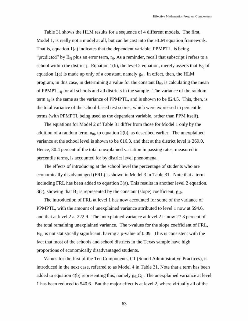
Effective Mathematics Program Components
63
Table 31 shows the HLM results for a sequence of 4 different models. The first,
Model 1, is really not a model at all, but can be cast into the HLM equation framework.
That is, equation 1(a) indicates that the dependent variable, PPMPTL, is being
―predicted‖ by B0j plus an error term, rij. As a reminder, recall that subscript i refers to a
school within the district j. Equation 1(b), the level 2 equation, merely asserts that B0j of
equation 1(a) is made up only of a constant, namely g00. In effect, then, the HLM
program, in this case, in determining a value for the constant B0j, is calculating the mean
of PPMPTLij for all schools and all districts in the sample. The variance of the random
term rij is the same as the variance of PPMPTL, and is shown to be 824.5. This, then, is
the total variance of the school-based test scores, which were expressed in percentile
terms (with PPMPTL being used as the dependent variable, rather than PPM itself).
The equations for Model 2 of Table 31 differ from those for Model 1 only by the
addition of a random term, u0j, to equation 2(b), as described earlier. The unexplained
variance at the school level is shown to be 616.3, and that at the district level is 269.0,
Hence, 30.4 percent of the total unexplained variation in passing rates, measured in
percentile terms, is accounted for by district level phenomena.
The effects of introducing at the school level the percentage of students who are
economically disadvantaged (FRL) is shown in Model 3 in Table 31. Note that a term
including FRL has been added to equation 3(a). This results in another level 2 equation,
3(c), showing that B1 is represented by the constant (slope) coefficient, g10.
The introduction of FRL at level 1 has now accounted for some of the variance of
PPMPTL, with the amount of unexplained variance attributed to level 1 now at 594.6,
and that at level 2 at 222.9. The unexplained variance at level 2 is now 27.3 percent of
the total remaining unexplained variance. The t-values for the slope coefficient of FRL,
B1j, is not statistically significant, having a p-value of 0.09. This is consistent with the
fact that most of the schools and school districts in the Texas sample have high
proportions of economically disadvantaged students.
Values for the first of the Ten Components, C1 (Sound Administrative Practices), is
introduced in the next case, referred to as Model 4 in Table 31. Note that a term has been
added to equation 4(b) representing this, namely g01C1j. The unexplained variance at level
1 has been reduced to 540.6. But the major effect is at level 2, where virtually all of the

Effective Mathematics Program Components
64
remaining level 2 variance has been eliminated. Note that although the p-value for the
level 1 slope coefficient associated with FRL is still 0.092, that for the level 2 coefficient
g00, associated with C1, is 0.022, which is quite significant.
Each of the other components were substituted for C1 (Sound Administrative
Practices) in level 2 (equation 4(b) in Model 4 of Table 31), and the same calculations
carried out. These results, as well as those already shown in Table 31, are summarized in
Table 32. It appears that several of the other Ten Components would also account for
most of the level 2 variance, most notably C2 (Aligned Curriculum), C3 (Ongoing
Assessment), C7 (Instructional Materials and Teaching Techniques), and C8
(Differentiated Instruction), with C6 (Teacher Knowledge of Mathematics Content) and
C9 (Focused Professional Development) also statistically significant.
The component which fares least well is C10 (End-of-Year Analysis). Since all
districts in Texas, by statute, perform end of year testing in math, this component should
not be expected to explain differences among school districts.

Effective Mathematics Program Components
65
Table 32
Summary of HLM Calculations with Each of the Ten Components
Used Separately as District Level Independent Variable
FRL
Component
Used
p-values Unexplained
Variance
Degrees
of Freedom
FRL Cj Lev 1 Lev 2 Lev 1 Lev 2
1 824.5 39
2 616.3 269.0 39 5
3 x .090 594.6 222.9 38 5
4 x C1 .092 .022 540.6 0.1 37 4
5 x C2 .155 .034 577.7 0.5 37 4
6 x C3 .378 .034 580.7 0.3 37 4
7 x C4 .022 .065 602.4 51.3 37 4
8 x C5 .203 .160 593.0 135.5 37 4
9 x C6 .028 .044 590.7 26.9 37 4
10 x C7 .079 .032 570.1 0.4 37 4
11 x C8 .019 .032 570.6 0.6 37 4
12 x C9 .173 .039 594.6 5.2 37 4
13 x C10 .107 .574 594.4 270.6 37 4
Note: In row 2 the stochastic level 2 intercept, u0j, was added. Results in the first 4 rows also shown in Table 31.
The value of these results can be illustrated visually, using the framework established
when discussing the methods used to select districts for inclusion in the study (Section 4
above). The MMRs for the districts included in this study are plotted in Figure 9, with
FRL on the horizontal axis. While there seems to be some stratification to the pattern, the
correlation coefficient between the variables is just –0.13, and is quite insignificant, with
a significance value of 0.806. However, when those original MMRs (obtained using
elementary and middle school campuses in most districts in the state) are plotted against
the C1 (Sound Administrative Practices) values obtained from the survey results they fall
into a pronounced linear pattern, as can be observed in Figure 10. The correlation

Effective Mathematics Program Components
66
coefficient between the original MMRs and the survey-derived C1 (Sound Administrative
Practices) is 0.949, with a significance value of 0.004.
Figure 9
District Performance Measures v Percent Low Income Students
Figure 10
District Performance Measures v Values for Component 1

Effective Mathematics Program Components
67
The results of plotting the MMRs which were derived by using data only from the
schools and school districts in the sample against the C1 values are even more striking, as
shown in Figure 11. Even though only 6 school districts were included in this study, the
relationship between C1 (Sound Administrative Practices) and the school district
performance measures (MMRs) appears very strong. Similar patterns are obtained using
the values associated with C2 (Aligned Curriculum), C3 (Ongoing Assessment), C6
(Teacher Knowledge of Mathematics Content), C7 (Instructional Materials and Teaching
Techniques), and C8 (Differentiated Instruction) as well.
Figure 11
District Performance Measures v Component 1

Effective Mathematics Program Components
68
Section 8: Relationship between student performance, proportion of
economically disadvantaged students, and test difficulty—three states
The discussion in Section 4 built upon observations made with respect to the scatter
plot of school performance versus percent economically disadvantaged students, as
shown in Figure 1 for North Carolina. Before proceeding with the statistical analysis
based on data from all 3 states, diagrams similar to Figure 1, but for California and
Texas, will be compared to that for North Carolina. The diagrams for all three states are
shown in Figures 12, 13, and 14. North Carolina data are plotted again in Figure 12.
Similar plots are shown for Texas (Figure 13) and California (Figure 14).
As stated earlier, the campus performance measure used for North Carolina, and used
in the scatterplot in Figure 12, was the percentage of students in all grades of each school
whose math scaled score was above the cutoff value for Level III. This is the measure
used in North Carolina to determine whether students are performing adequately or not.
The performance measure used in plotting the Texas schools shown in Figure 13 was
based on the percentage of students who achieved the passing score or better on the 2002
TAAS. The regression line shown in the scatterplot for Texas is noticeably higher and
less steep than the one shown for North Carolina. This suggests that, on average, a
higher proportion of students in Texas schools achieve the TAAS passing level than is the
case in North Carolina for the proportion of students who achieved Level III or higher.
In both states it appears that schools with extremely low proportions of economically
disadvantaged students were hitting the ceiling. The net result is a much weaker apparent
relationship between poverty and academic performance in Texas than in North Carolina.

Effective Mathematics Program Components
69
Figure 12
North Carolina Elementary and Middle Schools, 2002
Figure 13
Texas Elementary and Middle Schools, 2002
Figure 14
California Elementary and Middle Schools, 2002

Effective Mathematics Program Components
70
Turning to California, as represented in Figure 14, the inverse relationship between
poverty and school performance is at least as strong as in North Carolina. In addition,
there appears to be even greater remaining variance around the regression line in the
California data than in the North Carolina data. It is important to note that the criterion
for ―passing‖ applied to the campus performance measures used in creating the
scatterplot in Figure 14 was that students get a score on the CCS math test at or above a
level labeled ―Basic‖. California divides performance domains into the four classes:
Advanced, Proficient, Basic, Below Basic.
It is interesting and instructive to create scatterplots for California schools using each
of two additional criteria, namely student performance at or above Proficient, and also at
or above Below Basic. The scatterplots for California schools based on all three criteria
are shown in Figure 15, graphs A, B, and C. Figure 15-A used the performance criterion
of ―equal to or greater than Below Basic‖, Figure 15-B reflects performance ―equal to or
greater than Basic‖, and Figure 15-C is based on performance ―equal to or greater than
Proficient‖. The ordinary least-squares slopes of these three relationships are presented
in Table 33.
The implication of these slopes can be stated as follows. Compared to a typical
school with no ED students, a school with 100 percent ED students would have a pass
rate 11 percent lower (graph A), 36 percent lower (graph B), or 42 percent lower (graph
C). Two of these comparisons represent very large differences in school performance
and major differences in the achievement gap between high-poverty and low-poverty
schools. Using the Below Basic criterion, it appears that most California elementary and
middle schools are doing quite well, and that most of the achievement gap between low
income and high income schools has been eliminated. But if the same tests, administered
to the same students in each of the schools, are scored using either the Basic or the
Proficient criterion, the remaining gap between extreme low income and extreme high
income schools would be several times greater—36 or 42 percentage point differences, as
opposed to only an 11 point difference using the Below Basic criterion.

Effective Mathematics Program Components
71
Figure 15
California Elementary and Middle Schools, 2002
Three Different Assessment Criteria
Graph A: Percent at or above ―Below Basic‖
Graph B: Percent at or above ―Basic‖
Graph C: Percent at or above ―Proficient‖

Effective Mathematics Program Components
72
Table 33
Slopes of Regression Lines, Figures 8-A, 8-B, 8-C
Relationship shown in Slope Coefficient t-value
Figure 8-A -0.107 -59.5
Figure 8-B -0.359 -82.4
Figure 8-C -0.420 -81.6
Another aspect of the effects of using different criteria on the same test to declare
―proficiency‖ is that the total variance to be explained decreases with a less demanding
criterion, and the variance remaining after taking into consideration ED is divided
differently between the campus level and the district level. This is illustrated for the three
California cases, presented in Table 34.
Table 34
California Elementary and Middle Schools, Grades 2 through 7
Allocation of Variance between Campus and District
Using Three Different Performance Criteria
Variance
Equal or exceed
Proficient
Equal or exceed
Basic
Equal or exceed
Below Basic
Campus 100.2 76.3 14.3
District 63.7 33.9 3.3
Pct. District 38.9% 30.6% 19.8%
This observation is relevant to the analysis above (Sections 5 – 7) where it was
attempted to assess which district operational practices explain why schools in some
districts perform better than those in other districts. If a low cutoff score is used to
determine the percentage of students who achieve the target level of competency then it
will be less likely that effective policies, at either the district or school level, can be
identified. For example, in an extreme case, all schools would be assessed as performing
equally well. In such an instance, it would not matter that different schools used different
teaching practices or had other program differences. If it does matter which programs are

Effective Mathematics Program Components
73
used and how they are implemented, the effects of variations in programs cannot be
determined. This situation would result if the assessment test is so easy, or scored so
leniently, that all schools appear to be performing equally well.
Another manifestation of the effects of applying different threshold levels in
evaluating student success is the impact on the frequency distribution of schools with
various percentages of pass rates. The histograms based on the same data used in
constructing the scatterplots of Figure 15 are shown in Figure 16. Note the overall
average school passing rates associated with each histogram (Mean scores). The average
passing rate using the Below Basic criterion was 94 percent. Using the Basic criterion
the average passing rate was just 71 percent. And using the toughest criterion, the
Proficient measure, the average passing rate was just 41 percent.18
The comparable histogram for the North Carolina and Texas pass rates that were
used in constructing Figures 12 and 13 are shown in Figure 17. Note the similarity in the
shapes of the histogram for Texas (Figure 17-B) and California, when the Below Basic
criterion of students success is used in the latter state (Figure 16-A).
Unlike the California Department of Education the Texas Education Agency does not
post Texas TAAS results with alternate passing criteria. Therefore, in Section 9 below,
where Texas’ data are combined with those for North Carolina and California, the Texas
school performance measures based on the Percent Passing the TAAS Math test will
necessarily be used. All analyses involving the California data will utilize the school
success measure based on the Basic level of competence, and for North Carolina the
school success measure will be based on achieving Level III.

Effective Mathematics Program Components
74
Figure 16
Distributions of Passing Rates among California Elementary and
Middle Schools under Three Different Assessment Standards—2002
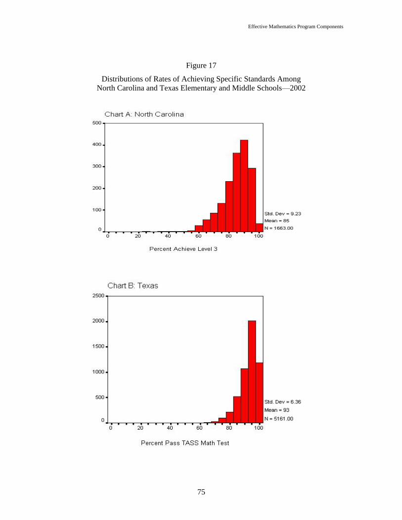
Effective Mathematics Program Components
75
Figure 17
Distributions of Rates of Achieving Specific Standards Among
North Carolina and Texas Elementary and Middle Schools—2002

Effective Mathematics Program Components
76
Section 9: Multi-State Analysis—California, North Carolina, and Texas
Following from the previous discussion, even with the potential problems inherent in
any attempt to combine data from three different systems, we may be able to accomplish
a more powerful analysis through the grouping of the merged data from California, North
Carolina and Texas. There are obvious differences in the data for the three states. The
schools in Texas tended to have higher passing rates and greater proportions of students
classified as economically disadvantaged than the schools in North Carolina and
California. Those differences can be seen in Figure 18, where percent pass rates and
percent economically disadvantaged for each school in the sample are plotted.
Figure 18
10080604020
PERCENT ECONOMICALLY DISADVANTAGED
100
90
80
70
60
50
40
30
PC
T P
AS
S M
AT
H
CA
TX
NC
STATE
EACH STATE CRITERION FOR MATH PASS RATE

Effective Mathematics Program Components
77
Because the average pass rates differ by state (see Figures 16-B, 17-A, and 17-B)
some adjustment was required. The pass rates were converted to z-scores (and multiplied
by 100) for the schools, on a state-by-state basis. This gave a mean of zero and a
standard deviation of 100 for the performance measures of schools in each state. Figure
19 shows the relation between the original pass rates (horizontal axis) and the resulting z-
scores (vertical axis).
Figure 19
Plotting the z-scores for performance against the percent of economically
disadvantaged students (Figure 20) shows a somewhat more homogenous picture, but the
higher rate of poor students in Texas is clearly evident. The simple means of the campus
percentages of economically disadvantaged students, by state, are: Texas 79%;
California 65%; North Carolina 60%.

Effective Mathematics Program Components
78
Figure 20
10080604020
PERCENT ECONOMICALLY DISADVANTAGED
300
200
100
0
-100
-200
-300
PE
RC
EN
T P
AS
S M
AT
H, S
TA
TE
Z-S
CO
RE
S
CA
TX
NC
STATE
PASS MATH (Z-SCORES) v PERCENT ECONOMICALLYDISADVANTAGED
HLM was used to determine the modified mean residuals (MMRs) for each of the 18
districts represented in the combined data set. Recall the MMRs are measures of district
academic performance. The correlation coefficients between the MMRs and the average
value for each component, by school, are presented in Table 35. As can be seen there, 9
of the 10 correlation coefficients are significant, with 6 of them significant at the 0.01
level. The greatest correlation was associated with C1 (Sound Administrative Practices),
again suggesting its importance as perhaps a necessary condition for implementing the
other practices associated with higher student performance.

Effective Mathematics Program Components
79
Table 35
CORRELATIONS--DISTRICT PERFORMANCE AND TEN
COMPONENTS, THREE STATES MERGED DATA
.794**
.000
.761**
.000
.734**
.000
.335
.087
.402*
.049
.590**
.005
.661**
.001
.443*
.033
.530*
.012
.557**
.008
Pearson Correlation
Sig. (1-tailed)
Pearson Correlation
Sig. (1-tailed)
Pearson Correlation
Sig. (1-tailed)
Pearson Correlation
Sig. (1-tailed)
Pearson Correlation
Sig. (1-tailed)
Pearson Correlation
Sig. (1-tailed)
Pearson Correlation
Sig. (1-tailed)
Pearson Correlation
Sig. (1-tailed)
Pearson Correlation
Sig. (1-tailed)
Pearson Correlation
Sig. (1-tailed)
c1_tpa
c2_tpa
c3_tpa
c4_tpa
c5_tpa
c6_tpa
c7_tpa
c8_tpa
c9_tpa
c10_tpa
MMR
(SCHOOL
Z-SCORES)
Correlation is significant at the 0.01 level (1-tailed).**.
Correlation is significant at the 0.05 level (1-tailed). N = 18*.
To further illustrate the pattern of association between individual components and
district performance (MMR), a series of figures that chart several of the Ten Components
whose values were derived from the merged data, plotted against the modified mean
residuals (MMR), are presented. For comparison purposes, the data points are also
distinguished by state.
Figure 21 highlights the strong relationship between the district performance measure
and Component 1 (Sound Administrative Practices). Note the extremely small range for
the average school values for Component 1 for North Carolina’s schools. Smaller charts
showing similar information for Components 1, 2, 3, and 7 are displayed in Figure 22.

Effective Mathematics Program Components
80
Figure 21
4.64.44.24.03.83.63.43.2
COMPONENT 1 (C1_TPA)
80
60
40
20
0
-20
-40
-60
-80
DIS
TR
ICT
PE
RF
OR
MA
NC
E (
MM
R_M
3)
CA
TX
NC
STATE
DISTRICT PERFORMANCE v ADMINISTRATIVE PRACTICES
CALIF, TEXAS, N. CAROLINA
The responses to most questions in the survey required responses on a 1 to 5 scale,
but there were some systematic differences among the 3 states when the responses were
averaged, by component, to the district level. First, there was a smaller variance by
respondents in North Carolina for most of the Ten Components. Ignoring C5 (Increased
and Effective Use of Instructional Time) (which was not based on a 1 to 5 scale) districts
in North Carolina showed a smaller standard deviation for 7 of the 9 components. This is
reflected clearly in Figure 21, for component 1. The other noticeable feature of the
district level averages of these 9 components is that the mean values for the Texas
districts are higher than those for North Carolina and California in eight of the nine cases,
with North Carolina and Texas tied in the case of component 7. These means and
standard deviations, by state by component, are displayed in Table 36.

Effective Mathematics Program Components
81
Figure 22
c7_tpac3_tpac2_tpac1_tpammr_m3
mm
r_m
3c1_
tpa
c2_
tpa
c3_
tpa
c7_
tpa
CA
TX
NC
STATE
CALIF, TEXAS, NORTH CAROLINA
COMPONENTS 1, 2, 3, AND 7 PLOTTED AGAINST DISTRICT PERFORMANCE
The strong associations reported in Table 35 and shown in Figures 21 and 22,
based on the merged data from the 3 states, should be viewed with some caution. The
higher average poverty rates and higher test passing rates would tend to cause the district
performance measures (MMRs) to be greater for Texas districts. In addition, the average
of the district-level component scores was higher for eight components in the Texas
districts than those in the other two states (see Table 36). These two factors might bias
the distributions seen in Figures 21 and 22 and the correlation coefficients in Table 35. It
is not known why the average responses to the survey questions were higher in Texas for
8 of the 9 components which used the 1 – 5 response scale (and tied for one more). One
possibility is that the higher pass rates in Texas are related to real higher student
achievement which in turn is related to more intensive implementation of the Ten
Components. In this case the higher average component scores in Texas would accurately
reflect teacher and principal responses regarding implementation of them. Another
possibility is that the higher pass rates in Texas might be due to a less difficult test or a

Effective Mathematics Program Components
82
lower cut-off score for passing and the higher judgments on the survey instruments
spurious. In short, why would the responses in different states be systematically
different? This question needs to be addressed in designing any future interstate studies
of this type where multi-state pooling of such information would occur.
Table 36
MEANS AND STANDARD DEVIATIONS OF DISTRICT AVERAGE COMPONENT VALUES
State Component Mean Max
Mean Std. Deviation Min. Std. Deviation
NC C1 3.93 0.052 **
NC C2 4.09 0.105 **
NC C3 3.84 0.074 **
NC C4 2.26 0.294
NC C6 3.81 0.135 **
NC C7 4.43 ** 0.082 **
NC C8 3.74 0.219 **
NC C9 3.20 0.120 **
NC C10 3.97 0.151
TX C1 4.18 ** 0.251
TX C2 4.17 ** 0.295
TX C3 4.22 ** 0.225
TX C4 2.58 ** 0.408 **
TX C6 4.40 ** 0.233
TX C7 4.43 ** 0.276
TX C8 4.06 ** 0.238
TX C9 3.78 ** 0.306
TX C10 4.12 ** 0.151
CA C1 3.78 0.297
CA C2 4.13 0.364
CA C3 3.85 0.265
CA C4 1.10 0.078
CA C6 3.41 0.500
CA C7 4.13 0.362
CA C8 3.38 0.320
CA C9 3.14 0.149
CA C10 4.08 0.157 **

Effective Mathematics Program Components
83
Table 37
Hierarchical Linear Model Results, Three States
HLM Equations
Significance
(p-values)
Unexplained
Variance
Level 2
Pct
Variance
Deg. of
Freedom
FRL Cj Lev.
1
Lev.
2
Lev.
1
Lev.
2
Model 1
Level 1
(a) ZPPM = B0j + rij
Level 2
(b) B0j = g00
9810
105
Model 2
Level 1
(a) ZPPM = B0j + rij
Level 2
(b) B0j = g00 + u0j
8101
1860
18.7%
105
17
Model 3
Level 1
(a) ZPPM = B0j +B1FRLij+ rij
Level 2
(b) B0j = g00 + u0j
(c) B1 = g10
.000
6589
1876
22.2%
104
17
Model 4
Level 1
(a) ZPPM = B0j +B1FRLij+ rij
Level 2
(b) B0j = g00 + g01C1_TPAj + u0j
(c) B1 = g10
.000
.000
6574
16
0.2%
103
16
Model 5
Level 1
(a) ZPPM = B0j +B1FRLij+ rij
Level 2
(b) B0j = g00 + g01C1_TPAj
+ g02C2_TPAj
+ u0j
(c) B1 = g10
.000
.001
.008
6465
14
0.2%
102
15

Effective Mathematics Program Components
84
The HLM results for the combined data are presented in Table 37. The analysis is
analogous to that of the individual state analyses presented previously (Tables 11, 20, and
31). Model 1(Table 37) indicates that the total variance is 9,810, and Model 2 shows that
18.7 percent of this variance is attributable to differences among districts. In Model 3
FRL (percent of students eligible for federally-subsidized free or reduced-price lunches)
is used as an explanatory variable at the school level (level 1). This reduces the Level 1
variance from 8,101 to 6,589, leaving 22.2 percent of the remaining variance at the
district level.
In Model 4 Component 1 (Sound Administrative Practices) is used to explain level 2
variance. Inclusion of this variable almost completely eliminates the remaining level 2
variance (from 1,876 to 16). In Model 5, a second variable was added to explain level 2
variance, namely Component 2 (Aligned Curriculum). Both C1 and C2 were statistically
significant. It is likely that C3 (Ongoing Assessment) and C7 (Instructional Materials
and Teaching Techniques) would have similar ability to account for the district-level
variance, based upon their correlations with student performance (see Table 36). The
same caution expressed earlier regarding possible biases inherent in the merging of the
data from all three states, however, should be heeded in interpreting these results.
Section 10: Summary and Conclusions
The Ten Components of Effective Schools has been honed by Dr. Douglas Carnine
and others into a working definition of what behaviors good schools and school systems
should exhibit. The main purpose of this study was to see if a questionnaire-based data
gathering process could capture information adequate to help assess the efficacy of the
Ten Components. In that regard these pilot results seem quite promising. Districts and
schools were selected which had large proportions of economically disadvantaged
students, as these are the students who tend to be most at risk and which provide the
greatest challenges to our public schools.
Initially we presented the findings for each state separately. First, correlation and
linear regression analyses were used to see which of the Ten Components were
associated with the more successful schools, leaving aside district influence. Second,
using HLM, the district-level aggregates derived from the survey data were used to

Effective Mathematics Program Components
85
determine which of the components were most strongly associated with higher than
predicted performance among the school districts in the sample. Finally, we combined the
data across the states to get a better picture of the predictive value of the ten components
on a larger scale.
For North Carolina, the results were not too promising. The lack of variance between
schools and a smaller sample perhaps hampered our exploration efforts. For example, in
Table 20, Model 3 (which allows for effects of various proportions of economically
disadvantaged students) only 9 percent of the remaining variance was at the interdistrict
level. This made it quite difficult to detect the effects of variations in district policies
upon school performance. In addition, there may also have been some differences in the
methods employed to collect the data in North Carolina, which would account for the
lesser amount of variation in response to the survey questions.
A final factor at play in the case of North Carolina is that none of the five districts
that ultimately agreed to participate in the study was a high-performing district. As
shown in Figure 7 above, two of the five North Carolina districts appear to be high-
performing. But using data for all districts in North Carolina, none of those that
participated were high-performing, in relation to other North Carolina districts. Although
there was a good spread—two were average, two low, and one very low—the lack of one
or more truly high-performing districts meant that the survey data were without the
presumably higher ratings that would have been given by the personnel at such a district.
This may account for the diminished spread in the average Ten Component scores found
for North Carolina (See Table 36) and for at least part of the less definitive results found
there.
In California, the association between the components as measured by the teacher and
principal surveys and performance on the mathematics portion of the California
Standards Test showed a strong pattern of positive relationships. For teachers, six
components –C1 (Sound Administrative Practices), C2 (Aligned Curriculum), C4
(Immediate Intervention), C7 (Instructional Materials and Teaching Techniques), C9
(Focused Professional Development), C10 (End of Year Analysis of Student
Performance) – were significantly linked to basic and proficient performance levels on
the test. In addition, the linkage was stronger for proficient than for the basic level.

Effective Mathematics Program Components
86
Results gathered from principals reinforced the teachers’ perceptions as C1 (Sound
Administrative Practices), C2 (Aligned Curriculum), C6 (Teacher Knowledge of
Mathematics Content), and C7 (Instructional Materials and Teaching Techniques) were
correlated with assessment outcomes. When teacher and administrator views were
combined to create a school-level view, five components -- C1 (Sound Administrative
Practices), C2 (Aligned Curriculum), C7 (Instructional Materials and Teaching
Techniques), C9 (Focused Professional Development), and C10 (End of Year Analysis of
Student Performance)-- yielded significant correlations with test performance, and two
additional components -- C4 (Immediate Intervention), C6 (Teacher Knowledge of
Mathematics Content) -- showed a trend towards a significant relationship with
performance outcomes. The Ten Components were also strongly associated with
mathematics proficiency at the district level. Seven of the Ten Components — C1 (Sound
Administrative Practices), C2 (Aligned Curriculum), C3 (Ongoing Assessment), C4
(Immediate Intervention), C6 (Teacher Knowledge), C7 (Instructional Materials and
Teaching Techniques), C10 (End of Year Analysis of Student Performance)
demonstrated moderate to strong correlations with performance on California’s
Mathematics Test.
At the school level, all of the components are positively related, with nine
significantly correlated to the majority of the other components. In other words, if a
school scores high on one component, scores on the other components are likely to be
high as well.
For Texas, we also found some interesting patterns in the data. At the school level,
when we used teachers’ data we saw a fairly consistent pattern of relationships between
the components but little relation to outcome variables. While the estimated values of the
Ten Components themselves were fairly highly correlated with each other, none were
significantly correlated with student performance as measured by the percentage of
students tested who passed the state mandated TAAS Mathematics Test (PPM) in 2002.
Based upon the data obtained from the principals at the same schools, the intercorrelation
among estimates for the extent of implementation of the Ten Components was also fairly
high—32 of the 45 possible pairs of correlation coefficients were significant at the 0.05
level or better. In addition, four of the components were significantly correlated with
Effective Mathematics Program Components
87
PPM, namely C6 (Teacher Knowledge of Mathematics Content), C7 (Instructional
Materials and Teaching Techniques), C8 (Differentiated Instruction), and C9 (Focused
Professional Development).
When estimated values of the extent of implementation of the Ten Components were
calculated by combining those derived from teachers and principals into single measures,
the resulting measures were more highly correlated with one another than were those
derived from teacher and principal data taken separately. In addition, six of the
components were significantly correlated with student performance—C1 (Sound
Administrative Practices), C3 (Ongoing Assessment), C6 (Teacher Knowledge of
Mathematics Content), C7 (Instructional Materials and Teaching Techniques), C8
(Differentiated Instruction) and C9 (Focused Professional Development)—using the
percentile rank measure of the percentage of students passing the mathematics test. The
teacher-principal combined versions of the estimated values for the Ten Components
were used as explanatory variables in a regression equation. The results were that C1
(Sound Administrative Practices) and C6 (Teacher Knowledge of Mathematics Content),
along with economic disadvantage, were statistically significant, although C6 was only
marginally so with a p-value of 0.062. The suggestion here is that C1 tends to trump the
others. Indeed, it may be likely that effective administrative practices are necessary
before the Ten Components can be effectively implemented, even at the school level.
At the school district level, taken singly, seven of the Ten Components each
accounted for the vast majority of the unexplained interdistrict variation remaining after
taking into account the proportion of economically disadvantaged students at the school
level (Table 32). These consisted of C1 (Sound Administrative Practices), C2 (Aligned
Curriculum), C3 (Ongoing Assessment), C6 (Teacher Knowledge of Mathematics
Content), C7 (Instructional Materials and Teaching Techniques), C8 (Differentiated
Instruction), and C9 (Focused Professional Development). With only 4 degrees of
freedom remaining for district level variables with one of them included, it was not
considered possible to introduce more than one at a time. The high degree of consistency
between estimated values for C1 and the estimates of district performance was
remarkable (as illustrated in Figure 11). The two school districts in the upper-right-hand
portion of Figure 11 should feel proud of their accomplishments. These districts are

Effective Mathematics Program Components
88
commonly recognized as being outstanding with regard to student performance and
administrative energy and zeal. It speaks well for the survey used herein that these
districts ranked high in terms of implementation of the Ten Components, particularly C1,
which reflects over-all effective administrative practices.
Analyses utilizing data for all 3 states were somewhat more robust than the individual
state analyses. For example, 9 of the 10 components were significantly correlated with
the district measure of student performance. Only C4 (Immediate Intervention) failed to
qualify, but its significance level was still a fairly respectable 0.087. The high degree of
correlation between most of the Ten Components and the district performance measure
ensured that those components would be effective in accounting for interdistrict variance
using HLM.
In Section 8 it was suggested that tougher tests or higher passing thresholds might
make it more likely that meaningful relationships will be found between average campus
pass rates and various potential causal factors. Excessively demanding tests, with
extremely low pass rates would also prohibit identifying characteristics of the local
education program that enhance learning. It may be that California’s approach to
reporting school-level results is superior, in terms of facilitating analysis. Researchers
can choose whichever criterion for ―passing‖ is most useful, but a less severe standard
can be used for public recognition purposes. Ideally, the test results should not only
provide motivation for staff and students without being demoralizing, but they should
also provide critical data to researchers, including teachers and administrators, to help
identify those practices and programs that are most effective, and to discontinue those
that are ineffective. Also, in Section 9 we reviewed some of the problems that will be
encountered when trying to combine data collected in multiple states. While it might be
impossible to overcome some of these problems, the responses gathered here demonstrate
what might be gained if we compare across results states.
It is concluded that the data gathered from teachers and principals, reflecting their
opinion as to the degree of consistency of practices in their schools and school districts
with those described by the Ten Components of Effective Schools, lends strong support
to the importance of the Ten Components in improving student achievement. The survey
results seem most promising in explaining variations in the effectiveness of entire school

Effective Mathematics Program Components
89
districts. It is felt that the procedures described in this paper for measuring the
effectiveness of school districts are indeed useful in characterizing their differences. It
also appears that the survey instrument and methods employed in its use as described
herein are effective in measuring the extent of alignment of actual district and school
practices with the Ten Components.
The findings in this report are largely focused on school district performance. Yet
common sense suggests that learning actually occurs in the classroom under the tutelage
of the teacher. Critics frequently contend that funds not directed to the classroom are
generally wasted. Some states even have special restrictions on the proportion of total
funds which can be spent for district or school administration.
Recognition of the positive role of the school district in bringing about better student
performance in all schools in a district also means that proposals for hard upper limits to
the proportion of district funds that can be used for administrative purposes may not be
warranted, at least in the absence of an examination of the various administration
functions in promoting learning itself. Different districts may have different strategies as
to the relative size of the district educational activities as opposed to those at the school
level.
The school district, under the guidance of the board of supervisors and the
superintendent, makes the decisions that affect all schools, teachers, and pupils
throughout the district. In their book The Teaching Gap, Stigler and Hiebert (1999)
focused on mathematics teaching practices as recorded on videotape among 231 eighth
grade teachers in Germany, Japan, and the United States. They closely analyzed and
compared teachers’ practices in the 3 countries. They pointed out, for example, certain
characteristics of teaching found in Japan that might usefully be adopted in the U.S. But
in considering how U.S. teachers might be encouraged to adopt those practices, Stigler
and Hiebert proposed that such major change would probably have to be designed and
implemented by the school district administration. Only the district itself, they argued,
would have the authority and resources to carry out the planning and reallocation of
resources, especially teachers’ time, that would be necessary to implement and sustain
major improvements.19

Effective Mathematics Program Components
90
It is argued here that school district administrations in the more successful districts
included in this study have taken the lead in implementing district-wide adaptation of
their schools and teachers to respond successfully to the state-mandated accountability
systems. The Ten Components of Successful Schools appear to be beneficial if adopted,
and it seems that the school district has great influence over the degree to which these
practices are implemented. The findings reported above suggest that the school district is
critical in ensuring that whatever best practices are identified will be adopted and
supported throughout the district. These findings also suggest that the district influence
goes well beyond merely providing facilities, transportation, and other infrastructure. The
district is an active agent in the educational process itself.
Finally, the authors wish to express their gratitude to the many public school teachers
and administrators who volunteered some of their valuable time to participate in this
study. Without their help this would not be possible, and we hope that it can help us all
better understand practices and their relations to important outcomes.

Effective Mathematics Program Components
91
Bibliography
Aitkin, M., & Longford, N. (1986). ―Statistical modeling issues in school effectiveness
studies.‖ Journal of the Royal Statistical Society, Series A, 149(4), 1-43.
Bryk, A. & Raudenbush, S. W. (1992). Hierarchical Linear Models: Applications and
Data Analysis Methods. Newbury Park, CA: Sage.
Kane, T., Staiger, D. O., & Geppert, J. (2002). ―Randomly Accountable.‖ Hoover
Institution: Stanford. Available at http://www.educationnext.org/20021/56.html
Ma, L. (1999). Knowing and Teaching Elementary Mathematics. Mahwah, New Jersey:
Lawrence Erlbaum Associates.
National Research Council (2001). Adding it up: Helping Children Learn Mathematics.
Washington, DC: National Academy Press.
Raudenbush, S. W., & Bryk, A. (2002), Hierarchical Linear Models: Applications and
Data Analysis Methods (2nd
ed.). Newbury Park, CA: Sage.
Stigler, J. W., & Hiebert, J. (1999). The Teaching Gap: Best Ideas from the World’s
Teachers for Improving Education in the Classroom. New York: The Free Press.
Toenjes, L. A., &Garst, J. E. (2000). Identifying High Performing Texas Schools and
School Districts and Their Methods of Success. Report prepared for the Texas
Education Agency.
Toenjes, L. A., & Garst, J. E. (2002). Survey of Texas Reading Programs Based on the
Ten Components of Best Practice, Grades K – 8. Report prepared for the Texas
Education Agency.
Toenjes, L.A. Lewis, J. C. & Walne, M.B. (2003). Identifying Components of Effective
Mathematics Programs in Texas. Report prepared for the Texas Education Agency.
Thomas, Warren + Associates (2003). An Examination of School-Based Factors Affecting
the Grade 8 Mathematics MCAS Performance. Northampton, MA.
What Works Clearinghouse (2004). Topic report - Curriculum-based interventions for
increasing K-12 math achievement—middle school. Retrieved December 5, 2004
from http://whatworks.ed.gov/PDF/Topic/math_topic_report.html

Effective Mathematics Program Components
92
Appendix 1: State Questionnaires – California and Texas
DISTRICT OFFICE QUESTIONNAIRE OF
MATH PRACTICE, POLICY & INSTRUCTION
FOR GRADES 4-8
Please complete this questionnaire by using the below scale where appropriate and circling your response.
SD = Strongly Disagree; D = Disagree; U = Uncertain; A = Agree; SA = Strongly Agree
1. District Office Administrative Practices a) Our district provides written policies or guidelines for the
mathematics program.
SD D U A SA
b) Our district has written procedures for helping struggling
mathematics students reach grade level performance.
SD D U A SA
c) District instructional personnel visit each school regularly to
provide support for mathematics instruction
SD D U A SA
d) Administrative personnel provide feedback to each principal
about their school’s mathematics instruction.
SD D U A SA
e) When mathematics scores are not acceptable, a district
administrator visits that school to monitor improvement efforts.
SD D U A SA
2. Curriculum Alignment
a) Our district mathematics program has a written set of curriculum
guidelines for grades 4-8 based on the state mathematics standards.
SD D U A SA
District District Student Population
Name of Superintendent (or Director of Curriculum &
Instruction) completing this survey:
______________________________________
Position/Title___________________________________
Years Experience in This Position _______
Number of Teachers
District Economically Disadvantaged Percent District Mobility Rate

Effective Mathematics Program Components
93
3. Assessment
a) Our schools conduct mathematics assessments in grades 4-8
when the school year begins.
SD D U A SA
b) Our principals prepare regular student progress reports for
grades 4 through 8 in mathematics.
SD D U A SA
c) Periodic math assessment scores for every campus are made
available to all principals. SD D U A SA
d) Our principals meet with individual teachers regarding
their students’ performance scores in mathematics. SD D U A SA
SD = Strongly Disagree; D = Disagree; U = Uncertain; A = Agree; SA = Strongly Agree
4. Interventions for At-Risk Students a) Our district provides a continuum of services to meet the
individual needs of struggling mathematics students in grades 4-8.
SD D U A SA
b) Our district has a written list of services for students
needing additional support in math.
SD D U A SA
c) Our principals have available a written instructional plan for
each at-risk mathematics student in grades 4-8.
SD D U A SA
5. Instructional Time a) Our district requires a minimum number of minutes in
mathematics instruction per day that each child should receive.
If so, list the number of minutes by grade ________________
SD D U A SA
b) Our district prescribes the amount of extra mathematics
instruction a struggling mathematics student should receive during
each school day?
If so, list the number of minutes _____________
SD D U A SA
6. Teacher Knowledge of Mathematics Pedagogy a) All of our district grade 4 – 8 mathematics teachers must obtain
professional development in math annually.
SD D U A SA
b) The district monitors the professional development hours or
courses that each teacher attends annually.
SD D U A SA

Effective Mathematics Program Components
94
7. Instructional Materials and Teaching Techniques a) The mathematics program (for grades 4-8) in this district is
structured to emphasize depth of coverage. SD D U A SA
b) The mathematics program (for grades 4-8) in this district is
structured to emphasize breadth of coverage.
SD D U A SA
8. Grouping for Instruction
a) District math teachers (for grades 4-8) use flexible grouping (a
process for grouping and regrouping students based upon
performance).
SD D U A SA
9. Professional Development a) How often does your district provide training to principals in
effective mathematics program implementation? (please circle
response.)
Rarely,
if ever
Only with text
book adoption
Every
3-4
years
Every
1-2
years
b) Our principals provide time for mathematics teachers to plan
together by grade level during the school day.
SD D U A SA
SD = Strongly Disagree; D = Disagree; U = Uncertain; A = Agree; SA = Strongly Agree
9. Professional development (continued)
c) Mathematics specialists are available in our district to give
demonstration lessons and in-classroom assistance to math teachers
in grade 4-8.
SD D U A SA
d) Our principals provide mentoring and mathematics instructional
support for all teachers.
SD D U A SA
e) Our principals provide instructional support for teachers who are
not producing satisfactory gains in student performance.
SD D U A SA
10. End of Year Analysis of Student Performance (Grades 4-8) a) Our students take an annual assessment in mathematics that is a
national norm-referenced test.
SD D U A SA
b) Our students take an annual assessment in mathematics that is a
criterion-referenced test.
SD D U A SA
c) Our district makes annual data driven modifications to the
mathematics program for all schools.
SD D U A SA

Effective Mathematics Program Components
95
11. Open Ended Questions a) What is your district’s most serious problem in mathematics and how did you identify it?
b) What areas have you identified as needing improvement in the district mathematics program?
c) What is your district’s greatest success or discovery in math instruction?
Thank you for taking the time to complete this questionnaire.

Effective Mathematics Program Components
96
PRINCIPAL QUESTIONNAIRE OF
MATH PRACTICE, POLICY & INSTRUCTION
FOR GRADES 4-8
District School Name
Principal Name
Position/Title ____________________________
Years Experience as a Principal ______________
Grades Student Population
Economically Disadvantaged % Number of Teachers
Student Racial Composition:
Please complete this questionnaire by using the below scale where appropriate and circling your response.
SD = Strongly Disagree; D = Disagree; U = Uncertain; A = Agree; SA =
Strongly Agree
1. Administrative and Instructional Practices
a) Our district office provides written policies or guidelines for
the mathematics program.
SD D U A SA
b) How often do you observe in classrooms during
mathematics instruction?
Seldom
Once a
semester
Once a
month
Once a
week
Daily
c) How often does an assistant principal observe in classrooms
during mathematics instruction? Seldom Once a
semester
Once a
month
Once a
week
Daily
d) How often does a math skill specialist observe in classrooms
during mathematics instruction?
Seldom Once a
semester
Once a
month
Once a
week
Daily
e) Our math teachers receive individual feedback based on
observations of their teaching and their students’ performance
scores.
SD D U A SA
f) I meet regularly with the superintendent or our district
specialist to examine my school’s math scores.
SD D U A SA
g) Our teachers follow the state guidelines for math instruction
very closely.
SD D U A SA
h) I know who the at-risk math students are on our campus.
SD D U A SA
2. Curriculum Alignment
a) Our mathematics program has written curriculum guidelines
for each grade based on the state standards for mathematics. SD D U A SA

Effective Mathematics Program Components
97
b) If yes to (a) above, who writes the curriculum guidelines for
each grade?
District
Math
Coordinator
Textbook
Publishers
Teachers District
hired
experts
Other:_________________________________
____
SD = Strongly Disagree; D = Disagree; U = Uncertain; A = Agree; SA = Strongly Agree
Please circle your response.
2. Curriculum Alignment (Continued)
c) Our elementary and middle school math curricula are
coordinated so students are prepared for success in the
following grade.
SD D U A SA
3. Assessment a) A mathematics assessment is given to all students in grades
4-8 at the start of the year.
SD D U A SA
If yes to 3 (a) above, which assessment tools do you use at the start of each year for grades 4 through 8?
b) Our teachers use assessment data from the start of each
school year to identify students who may have difficulty
reaching grade level math standards.
SD D U A SA
c) Our grade level teachers give the same interim assessments
to determine student progress during the year.
SD D U A SA
d) Our teachers disaggregate performance data to determine
the areas students have and have not mastered.
SD D U A SA
e) Our grade level teachers meet regularly to discuss teaching
strategies.
SD D U A SA
f) Our grade level teachers meet regularly to discuss student
scores.
SD D U A SA
g) I receive mathematics assessment data throughout the year
from all teachers.
SD D U A SA

Effective Mathematics Program Components
98
h) I report interim student assessment data to the central
administrative office at least twice per year.
SD D U A SA
If yes to 3 (h) above, how does the district office use your math assessment scores?
i) Interim math test results for the other elementary (or middle)
schools in our district are made public. SD D U A SA
4. Interventions for At-Risk Mathematics Students
Extra instructional services for struggling math students at our school include (please check any that apply by grade):
a) Extra math instruction during the school day
a) Extra small group time in a pull-out program.
b) Tutoring.
c) An elective math class for students who need
remedial instruction
d) A required math class for students who need
remedial instruction
e) Other (please specify):_________________
_____________________________________
Grade: 4 ____ 5 _____ 6 _____ 7 _____ 8 _____
Grade: 4 ____ 5 _____ 6 _____ 7 _____ 8 _____
Grade: 4 ____ 5 _____ 6 _____ 7 _____ 8 _____
Grade: 4 ____ 5 _____ 6 _____ 7 _____ 8 _____
Grade: 4 ____ 5 _____ 6 _____ 7 _____ 8 _____

Effective Mathematics Program Components
99
b) Extra math instruction outside of the school day
a) Tutoring.
b) An extended day program.
c) An extended week program
d) Summer school.
e) Other (please specify):_________________
_____________________________________
Grade: 4 ____ 5 _____ 6 _____ 7 _____ 8 _____
Grade: 4 ____ 5 _____ 6 _____ 7 _____ 8 _____
Grade: 4 ____ 5 _____ 6 _____ 7 _____ 8 _____
Grade: 4 ____ 5 _____ 6 _____ 7 _____ 8 _____
Grade: 4 ____ 5 _____ 6 _____ 7 _____ 8 _____
c) Extra mathematics instruction is generally provided by (please check any that apply by grade):
a) Regular classroom teacher.
b) Teacher’s aid.
c) Skills specialist (certified teacher).
d) Certified teacher/tutor.
e) High school student.
f) Other (please specify):_________________
_____________________________________
Grade: 4 ____ 5 _____ 6 _____ 7 _____ 8 _____
Grade: 4 ____ 5 _____ 6 _____ 7 _____ 8 _____
Grade: 4 ____ 5 _____ 6 _____ 7 _____ 8 _____
Grade: 4 ____ 5 _____ 6 _____ 7 _____ 8 _____
Grade: 4 ____ 5 _____ 6 _____ 7 _____ 8 _____
Grade: 4 ____ 5 _____ 6 _____ 7 _____ 8 _____
d) Please list extra instructional services provided for special education students by grade. Who
generally provides the instruction?

Effective Mathematics Program Components
100
SD = Strongly Disagree; D = Disagree; U = Uncertain; A = Agree; SA = Strongly Agree
Please circle your response.
5. Instructional Time
a) How many minutes of mathematics instruction are provided during each school day for (Please fill-in number
of minutes for each grade that you are familiar.):
Grade: 4____ 5_____ 6_____ 7_____ 8_____
b) How much extra instructional time is provided to struggling math students during the school day for:
Grade: 4____ 5_____ 6_____ 7_____ 8_____
6. Teacher Knowledge of Mathematics Pedagogy
a) All of our mathematics teachers have been well trained to
teach math.
SD D U A SA
b) All of our mathematics teachers complete professional
development in math annually.
SD D U A SA
7. Instructional Materials and Teaching Techniques
a) Our instructional materials are based on the state standards
for mathematics.
SD D U A SA
b) Our math program covers (high-priority) state standards in
depth.
SD D U A SA
c) Our math instruction is paced so at least 90% of the students
have an opportunity to master prerequisite skills before moving
to more advanced concepts.
SD D U A SA
d) Our teachers provide practice time so at least 90% of the
students can develop proficiency in operations.
SD D U A SA
8. Grouping for Instruction
a) Our school provides sufficient math groups (or courses) to
meet all student abilities.
SD D U A SA
b) Most of our mathematics teachers provide instruction in
small groups based on student achievement results.
SD D U A SA
c) Most of our teachers use flexible grouping (a process for
grouping and regrouping students based on performance).
SD D U A SA

Effective Mathematics Program Components
101
SD = Strongly Disagree; D = Disagree; U = Uncertain; A = Agree; SA = Strongly Agree
Please circle your response.
9. Professional Development
a) Our mathematics teachers meet regularly within grades
during school hours.
SD D U A SA
b) Instructional resource personnel are available to give
demonstration lessons and in-class assistance to all
mathematics teachers.
SD D U A SA
c) The district office provides mathematics specialist(s) for the
schools in our district.
SD D U A SA
d) Our teachers attend workshops and visit other classrooms
during school time.
SD D U A SA
e) The instructional support that we provide to teachers having
difficulty is effective.
SD D U A SA
f) We have a mathematics specialist on our campus.
SD D U A SA
g) If yes to (f) above, on average how many hours does the
specialist(s) spend at your site weekly? (Please circle one or
specify other.)
Less than
10 hours
10-19
hours
20-29
hours
30-40
hours
Other:_________________________________
h) What type of mentoring do you provide new mathematics
teachers? (Please circle one or specify other.)
New teachers
work closely
with other
teachers
Each new
math teacher
is assigned a
mentor
The on-sight
skills specialist
mentors new
math teachers
Other:__________________________________
10. End of Year Analysis of Student Performance a) Our students take an end-of-year assessment in mathematics
that is a national norm-referenced test.
SD D U A SA
b) Annual data driven modifications are made to the
mathematics program on our campus.
SD D U A SA
c) Our campus has site based decision-making teams that study
the mathematics data to identify areas for improvement.
SD D U A SA

Effective Mathematics Program Components
102
d) Each teacher is expected to analyze student performance and
adjust their instruction accordingly.
SD D U A SA
e) Modifications to the mathematics program are primarily the
responsibility of the district office.
SD D U A SA
11. Open-ended Questions
a) Please identify what you consider to be your school’s most serious problem(s) in mathematics? How was this problem
identified?
b) What has been your school’s greatest discovery or success in math instruction?
Thank you for taking the time to complete this questionnaire.

Effective Mathematics Program Components
103
TEACHER QUESTIONNAIRE OF
MATH PRACTICE, POLICY & INSTRUCTION
FOR GRADES 4-8
Please complete this questionnaire by using the below scale where appropriate and circling your response.
SD = Strongly Disagree; D = Disagree; U = Uncertain; A = Agree; SA = Strongly Agree
1. Administrative Practices
a) Our district provides written policies or guidelines for the
mathematics program. SD D U A SA
b) My principal is knowledgeable about math instruction.
SD D U A SA
c) My principal closely monitors math performance at our
school. SD D U A SA
d) I feel valued as a math teacher at this school.
SD D U A SA
2. Curriculum Alignment a) Our math program is consistent with the state standards.
SD D U A SA
b) The mathematics teachers in our district make sure the
curriculum is coordinated so students are prepared for success
in the following grade. SD D U A SA
3. Assessment a) I assess all of my students at the beginning of the school
year in mathematics. SD D U A SA
b) I identify at-risk mathematics students from the assessment
results I collect at the beginning of the year.
SD D U A SA
c) I chart each at-risk student’s deficiencies in math.
SD D U A SA
d) I give ongoing assessments to track my students’ progress in
mathematics. SD D U A SA
e) I record each at-risk math student’s progress. SD D U A SA
f) I assess students’ mathematics computation skills twice a
week or more. SD D U A SA
g) My principal regularly receives a copy of my students’
assessment results.
SD D U A SA
h) Our grade level mathematics teachers give the same interim
assessments during the year.
SD D U A SA
i) Our grade level mathematics teachers meet regularly to
discuss assessment results.
SD D U A SA

Effective Mathematics Program Components
104
j) Our grade level mathematics teachers agree on what students
should be able to do to meet the state standards.
SD D U A SA
SD = Strongly Disagree; D = Disagree; U = Uncertain; A = Agree; SA = Strongly Agree
4. Interventions
a) Our school provides a continuum of services for at-risk
mathematics students.
SD D U A SA
b) Our programs for at-risk math students meet individual
student needs.
SD D U A SA
c) Which of the following services does your school provide for at-risk math students? (Please check services offered
and list others.)
_____ Extra small group time in a pull-out program
_____Before school tutoring
_____After school tutoring
_____Tutoring during the school day
_____Peer tutoring
_____An elective math class for students who need remedial instruction.
_____A required math class for students who need remedial instruction.
_____After-school classes.
_____Saturday classes.
_____Summer school
Other:________________________________________________________
d) Extra instruction for struggling math students is provided by
certified teachers.
SD
D
U
A
SA
e) Tutors (or others) that work with a struggling math student
are aware of that student’s specific learning needs.
SD D U A SA
f) I refer students who do not make progress in math for special
education testing.
SD D U A SA
g) I try different materials when a student is not making
progress in math.
SD D U A SA
h) When a student is not making progress in math, I conduct an
assessment to identify the problem. SD D U A SA

Effective Mathematics Program Components
105
i) I get help from a resource teacher when a student is not
making progress in math.
SD
D
U
A
SA
SD = Strongly Disagree; D = Disagree; U = Uncertain; A = Agree; SA = Strongly Agree
5. Instructional Time a) How many minutes of mathematics instruction are provided to students in your grade(s) during each school day?
Please list grade level(s) and minutes:_________
b) How many minutes of extra mathematics instruction are provided to your struggling mathematics students during
each school day?
Please list grade level(s) and minutes:_________
c) How many minutes of extra mathematics instruction are provided to your struggling mathematics students outside
the school day?
Please list grade level(s) and minutes:_________
6. Teacher Knowledge of Mathematics Pedagogy a) I attend professional development seminars on teaching
mathematics at least once per year.
SD D U A SA
b) My district provides substitutes so I can attend training held
during school hours.
SD D U A SA
7. Instructional Materials & Teaching Techniques a) I have curriculum guidelines in math from my district that
are keyed to the state standards.
SD D U A SA
b) I have instructional materials that are consistent with the
state mathematics standards.
Please list textbooks:______________________________
SD D U A SA
c) I use supplemental mathematics materials or programs.
Please list materials:______________________________
SD D U A SA
8. Grouping for Math Instruction a) I work with students in small groups.
SD D U A SA
b) I regularly use flexible grouping, where I group and regroup
students based upon performance.
SD D U A SA
9. Professional Development a) Professional development that improves my teaching of
math is available to me.
SD D U A SA

Effective Mathematics Program Components
106
b) The principal uses classroom observation to provide me with
feedback in teaching math.
SD D U A SA
c) The principal uses student math performance to provide me
with feedback in teaching math.
SD D U A SA
d) Mathematics teachers for my grade level have time to plan
together during the school day. SD D U A SA
SD = Strongly Disagree; D = Disagree; U = Uncertain; A = Agree; SA = Strongly Agree
e) Instructional resource personnel provide math demonstration
lessons and in-class assistance at our school. SD D U A
SA
f) Instructional resource personnel help me improve student
performance.
SD D U A SA
g) There is someone available to help me when I have
questions about teaching math.
SD D U A SA
10. End of Year Analysis a) In addition to the state test, I give an end-of-year assessment
in mathematics.
SD D U A SA
b) I make regular modifications to my teaching based on
student performance. SD D U A SA
c) I use annual test results to modify my instruction. SD D U A SA
1) District Name _______________________________
2) School Name ________________________________
3) Number of years teaching experience_____
10) Undergraduate degree(s)
a) Major(s)_______________________________
b) Minor(s)_______________________________
4) Type of certification(s) _________________________
___________________________________________
11) Graduate Degree(s)
a) Masters________________________________
5) Total Number of Math Classes You Teach _________
6) Total Number of Students You Teach _____________
b) Ed.D, Ph.D._____________________________

Effective Mathematics Program Components
107
7) Number of Math Classes of Each Type:
___ ESL ___ Bilingual
___ Low-Performing ___ GT or Honors
___ Special Ed ___ Regular (All student
levels)
Other_____________________________________
8) Grade(s) you are presently teaching: ____________
9) Type of instruction:
a) ___ Self-Contained
b) ___ Departmentalized
c) ___Team Teacher
d) ___Resource Teacher
e) Other ___________________________________
12) Mathematics Courses Taken in College (Check
those that apply)
a) ___ College Algebra
b) ___ Geometry
c) ___ Finite Math
d) ___ Trigonometry
e) ___ Calculus
f ) ___ Probability and Statistics
g) ___ Logic
h) Were the above math classes taken in a
department of mathematics?
___ yes ___ no ___ mixed
Thank you for taking the time to complete this survey.

Effective Mathematics Program Components
108
Appendix 1 (continued) – North Carolina Questionnaires
DISTRICT OFFICE QUESTIONNAIRE OF
MATH PRACTICE, POLICY & INSTRUCTION
FOR GRADES 4-8
Please complete this questionnaire by using the below scale where appropriate and circling your response.
SD = Strongly Disagree; D = Disagree; U = Uncertain; A = Agree; SA = Strongly Agree
1. District Office Administrative Practices a) Our district provides written policies or guidelines for the
mathematics program.
SD D U A SA
b) Our district has written procedures for helping struggling
mathematics students reach grade level performance.
SD D U A SA
c) District instructional personnel visit each school regularly to
provide support for mathematics instruction
SD D U A SA
d) Administrative personnel provide feedback to each principal
about their school’s mathematics instruction.
SD D U A SA
e) When mathematics scores are not acceptable, a district
administrator visits that school to monitor improvement efforts.
SD D U A SA
2. Curriculum Alignment
a) Our district mathematics program has a written set of curriculum
guidelines for grades 4-8 based on the state mathematics standards.
SD D U A SA
3. Assessment
ai) Our schools conduct mathematics assessments in grades 4-8
when the school year begins. SD D U A SA
aii) Our schools conduct mathematics assessments in grades 4-8
when the school year ends. SD D U A SA
b) Our principals prepare regular student progress reports for
grades 4 through 8 in mathematics.
SD D U A SA
District District Student Population
Name of Superintendent (or Director of Curriculum &
Instruction) completing this survey:
Position/Title:
Number of Teachers Years Experience in This Position :
District Economically Disadvantaged Percent District Mobility Rate

Effective Mathematics Program Components
109
c) Periodic math assessment scores for every campus are made
available to all principals. SD D U A SA
d) Our principals meet with individual teachers regarding
their students’ performance scores in mathematics.
SD D U A SA
SD = Strongly Disagree; D = Disagree; U = Uncertain; A = Agree; SA = Strongly Agree
4. Interventions for At-Risk Students a) Our district provides a continuum of services to meet the
individual needs of struggling mathematics students in grades 4-8.
SD D U A SA
b) Our district has a written list of services for students
needing additional support in math.
SD D U A SA
c) Our principals have available a written instructional plan for
each at-risk mathematics student in grades 4-8.
SD D U A SA
5. Instructional Time a) Our district requires a minimum number of minutes in
mathematics instruction per day that each child should receive.
If so, list the number of minutes by grade ________________
SD D U A SA
b) Our district prescribes the amount of extra mathematics
instruction a struggling mathematics student should receive during
each school day?
If so, list the number of minutes _____________
SD D U A SA
6. Teacher Knowledge of Mathematics Pedagogy a) All of our district grade 4 – 8 mathematics teachers must obtain
professional development in math annually.
SD D U A SA
b) The district monitors the professional development hours or
courses that each teacher attends annually.
SD D U A SA
7. Instructional Materials and Teaching Techniques a) The mathematics program (for grades 4-8) in this district is
structured to emphasize depth of coverage. SD D U A SA
b) The mathematics program (for grades 4-8) in this district is
structured to emphasize breadth of coverage.
SD D U A SA
9. Grouping for Instruction
a) District math teachers (for grades 4-8) use flexible grouping (a
process for grouping and regrouping students based upon
performance).
SD D U A SA

Effective Mathematics Program Components
110
9. Professional Development a) How often does your district provide training to principals in
effective mathematics program implementation? (please circle
response.)
Rarely,
if ever
Only with text
book adoption
Every
3-4
years
Every
1-2
years
b) Our principals provide time for mathematics teachers to plan
together by grade level during the school day.
SD D U A SA
SD = Strongly Disagree; D = Disagree; U = Uncertain; A = Agree; SA = Strongly Agree
9. Professional development (continued)
c) Mathematics specialists are available in our district to give
demonstration lessons and in-classroom assistance to math teachers
in grade 4-8.
SD D U A SA
d) Our principals provide mentoring and mathematics instructional
support for all teachers.
SD D U A SA
e) Our principals provide instructional support for teachers who are
not producing satisfactory gains in student performance.
SD D U A SA
10. End of Year Analysis of Student Performance (Grades 4-8) ai) Our students take an annual assessment in mathematics that is a
national norm-referenced test.
SD D U A SA
aii) Our students take an end-of-grade test in mathematics that is a
state norm-referenced test.
SD D U A SA
b) Our students take an annual assessment in mathematics that is a
criterion-referenced test.
SD D U A SA
c) Our district makes annual data driven modifications to the
mathematics program for all schools.
SD D U A SA

Effective Mathematics Program Components
111
11. Open Ended Questions b) What is your district’s most serious problem in mathematics and how did you identify it?
11. Open Ended Questions (continued) b) What areas have you identified as needing improvement in the district mathematics program?

Effective Mathematics Program Components
112
c) What is your district’s greatest success or discovery in math instruction?
Thank you for taking the time to complete this questionnaire.

Effective Mathematics Program Components
113
PRINCIPAL QUESTIONNAIRE OF
MATH PRACTICE, POLICY & INSTRUCTION
FOR GRADES 4-8
District School Name
Principal Name
Position/Title ____________________________
Years Experience as a Principal ______________
Grades Student Population
Economically Disadvantaged % Number of Teachers
Student Racial Composition:
Please complete this questionnaire by using the below scale where appropriate and circling your response.
SD = Strongly Disagree; D = Disagree; U = Uncertain; A = Agree; SA =
Strongly Agree
1. Administrative and Instructional Practices
a) Our district office provides written policies or guidelines for
the mathematics program.
SD D U A SA
b) How often do you observe in classrooms during
mathematics instruction?
Seldom
Once a
semester
Once a
month
Once a
week
Daily
c) How often does an assistant principal observe in classrooms
during mathematics instruction? Seldom Once a
semester
Once a
month
Once a
week
Daily
d) How often does a math skill specialist observe in classrooms
during mathematics instruction?
Seldom Once a
semester
Once a
month
Once a
week
Daily
e) Our math teachers receive individual feedback based on
observations of their teaching and their students’ performance
scores.
SD D U A SA
f) I meet regularly with the superintendent or our district
specialist to examine my school’s math scores.
SD D U A SA
g) Our teachers follow the state guidelines for math instruction
very closely.
SD D U A SA
h) I know who the at-risk math students are on our campus.
SD D U A SA

Effective Mathematics Program Components
114
2. Curriculum Alignment
a) Our mathematics program has written curriculum guidelines
for each grade based on the state standards for mathematics.
SD D U A SA
b) If yes to (a) above, who writes the curriculum guidelines for
each grade?
District
Math
Coordinator
Textbook
Publishers
Teachers District
hired
experts
Other:_________________________________
____
SD = Strongly Disagree; D = Disagree; U = Uncertain; A = Agree; SA = Strongly Agree
Please circle your response.
2. Curriculum Alignment (Continued)
c) Our elementary and middle school math curricula are
coordinated so students are prepared for success in the
following grade.
SD D U A SA
3. Assessment ai) A mathematics assessment is given to all students in grades
4-8 at the start of the year.
SD D U A SA
aii) A mathematics assessment is given to all students in grades
4-8 at the end of the year.
SD D U A SA
If yes to 3 (a) or 3 (b) above, which assessment tools do you use at the start and/or end of each year for grades 4
through 8?
b) Our teachers use assessment data to identify students
who may have difficulty reaching grade level math
standards.
SD D U A SA
c) Our grade level teachers give the same interim assessments
to determine student progress during the year.
SD D U A SA
d) Our teachers disaggregate performance data to determine
the areas students have and have not mastered.
SD D U A SA
e) Our grade level teachers meet regularly to discuss teaching
strategies. SD D U A SA

Effective Mathematics Program Components
115
f) Our grade level teachers meet regularly to discuss student
scores.
SD D U A SA
g) I receive mathematics assessment data throughout the year
from all teachers.
SD D U A SA
h) I report interim student assessment data to the central
administrative office at least twice per year.
SD D U A SA
If yes to 3 (h) above, how does the district office use your math assessment scores?
i) Interim math test results for the other elementary (or middle)
schools in our district are made public. SD D U A SA
4. Interventions for At-Risk Mathematics Students
Extra instructional services for struggling math students at our school include (please check any that apply by
grade):
a) Extra math instruction during the school day
a) Extra small group time in a pull-out program.
b) Tutoring.
c) An elective math class for students who need
remedial instruction
d) A required math class for students who need
remedial instruction
e) Other (please specify):_________________
_____________________________________
Grade: 4 ____ 5 _____ 6 _____ 7 _____ 8 _____
Grade: 4 ____ 5 _____ 6 _____ 7 _____ 8 _____
Grade: 4 ____ 5 _____ 6 _____ 7 _____ 8 _____
Grade: 4 ____ 5 _____ 6 _____ 7 _____ 8 _____
Grade: 4 ____ 5 _____ 6 _____ 7 _____ 8 _____
b) Extra math instruction outside of the school day
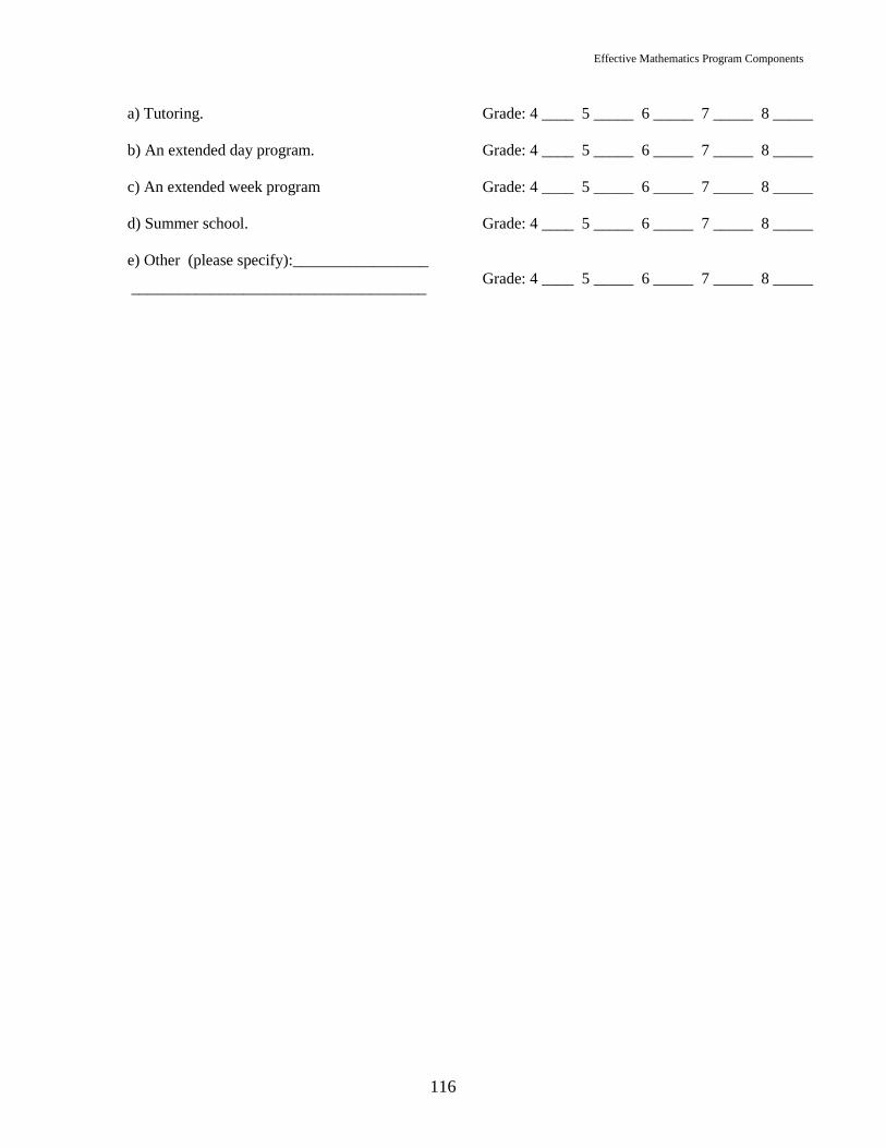
Effective Mathematics Program Components
116
a) Tutoring.
b) An extended day program.
c) An extended week program
d) Summer school.
e) Other (please specify):_________________
_____________________________________
Grade: 4 ____ 5 _____ 6 _____ 7 _____ 8 _____
Grade: 4 ____ 5 _____ 6 _____ 7 _____ 8 _____
Grade: 4 ____ 5 _____ 6 _____ 7 _____ 8 _____
Grade: 4 ____ 5 _____ 6 _____ 7 _____ 8 _____
Grade: 4 ____ 5 _____ 6 _____ 7 _____ 8 _____

Effective Mathematics Program Components
117
c) Extra mathematics instruction is generally provided by (please check any that apply by grade):
a) Regular classroom teacher.
b) Teacher’s aid.
c) Skills specialist (certified teacher).
d) Certified teacher/tutor.
e) High school student.
f) Other (please specify):_________________
_____________________________________
Grade: 4 ____ 5 _____ 6 _____ 7 _____ 8 _____
Grade: 4 ____ 5 _____ 6 _____ 7 _____ 8 _____
Grade: 4 ____ 5 _____ 6 _____ 7 _____ 8 _____
Grade: 4 ____ 5 _____ 6 _____ 7 _____ 8 _____
Grade: 4 ____ 5 _____ 6 _____ 7 _____ 8 _____
Grade: 4 ____ 5 _____ 6 _____ 7 _____ 8 _____
d) Please list extra instructional services provided for special education students by grade.
Who generally provides the instruction?
SD = Strongly Disagree; D = Disagree; U = Uncertain; A = Agree; SA = Strongly Agree
Please circle your response.
5. Instructional Time
a) How many minutes of mathematics instruction are provided during each school day for (Please fill-in number
of minutes for each grade that you are familiar.):
Grade: 4____ 5_____ 6_____ 7_____ 8_____
b) How much extra instructional time is provided to struggling math students during the school day for:
Grade: 4____ 5_____ 6_____ 7_____ 8_____
6. Teacher Knowledge of Mathematics Pedagogy
a) All of our mathematics teachers have been well trained to
teach math.
SD D U A SA
b) All of our mathematics teachers complete professional
development in math annually.
SD D U A SA
7. Instructional Materials and Teaching Techniques
a) Our instructional materials are based on the state standards
for mathematics.
SD D U A SA
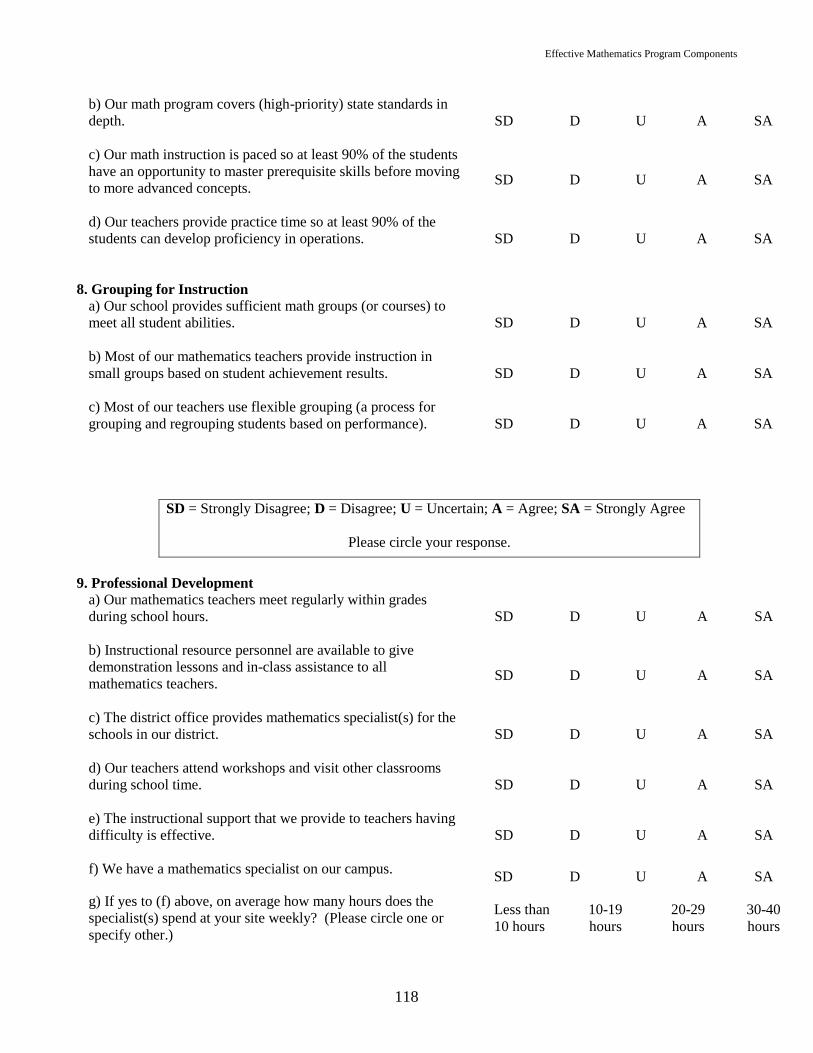
Effective Mathematics Program Components
118
b) Our math program covers (high-priority) state standards in
depth.
SD D U A SA
c) Our math instruction is paced so at least 90% of the students
have an opportunity to master prerequisite skills before moving
to more advanced concepts.
SD D U A SA
d) Our teachers provide practice time so at least 90% of the
students can develop proficiency in operations.
SD D U A SA
8. Grouping for Instruction
a) Our school provides sufficient math groups (or courses) to
meet all student abilities.
SD D U A SA
b) Most of our mathematics teachers provide instruction in
small groups based on student achievement results.
SD D U A SA
c) Most of our teachers use flexible grouping (a process for
grouping and regrouping students based on performance).
SD D U A SA
SD = Strongly Disagree; D = Disagree; U = Uncertain; A = Agree; SA = Strongly Agree
Please circle your response.
9. Professional Development
a) Our mathematics teachers meet regularly within grades
during school hours.
SD D U A SA
b) Instructional resource personnel are available to give
demonstration lessons and in-class assistance to all
mathematics teachers.
SD D U A SA
c) The district office provides mathematics specialist(s) for the
schools in our district.
SD D U A SA
d) Our teachers attend workshops and visit other classrooms
during school time.
SD D U A SA
e) The instructional support that we provide to teachers having
difficulty is effective.
SD D U A SA
f) We have a mathematics specialist on our campus. SD D U A SA
g) If yes to (f) above, on average how many hours does the
specialist(s) spend at your site weekly? (Please circle one or
specify other.)
Less than
10 hours
10-19
hours
20-29
hours
30-40
hours

Effective Mathematics Program Components
119
Other:_________________________________
h) What type of mentoring do you provide new mathematics
teachers? (Please circle one or specify other.)
New teachers
work closely
with other
teachers
Each new
math teacher
is assigned a
mentor
The on-sight
skills specialist
mentors new
math teachers
Other:___________________________________
10. End of Year Analysis of Student Performance ai) Our students take an end-of-year assessment in mathematics
that is a national norm-referenced test.
SD D U A SA
aii) Our students take an end-of-grade test in mathematics that
is a state norm-referenced test.
SD D U A SA
b) Annual data driven modifications are made to the
mathematics program on our campus.
SD D U A SA
c) Our campus has site based decision-making teams that study
the mathematics data to identify areas for improvement.
SD D U A SA
d) Each teacher is expected to analyze student performance and
adjust their instruction accordingly. SD D U A SA
e) Modifications to the mathematics program are primarily the
responsibility of the district office.
SD D U A SA
11. Open-ended Questions
a) Please identify what you consider to be your school’s most serious problem(s) in mathematics? How was this problem
identified?
b) What has been your school’s greatest discovery or success in math instruction?

Effective Mathematics Program Components
120
Thank you for taking the time to complete this questionnaire.

Effective Mathematics Program Components
121
TEACHER QUESTIONNAIRE OF
MATH PRACTICE, POLICY & INSTRUCTION
FOR GRADES 4-8
Please complete this questionnaire by using the below scale where appropriate and circling your response.
SD = Strongly Disagree; D = Disagree; U = Uncertain; A = Agree; SA = Strongly Agree
1. Administrative Practices
a) Our district provides written policies or guidelines for the
mathematics program. SD D U A SA
b) My principal is knowledgeable about math instruction.
SD D U A SA
c) My principal closely monitors math performance at our
school. SD D U A SA
d) I feel valued as a math teacher at this school.
SD D U A SA
2. Curriculum Alignment a) Our math program is consistent with the state standards.
SD D U A SA
b) The mathematics teachers in our district make sure the
curriculum is coordinated so students are prepared for success
in the following grade. SD D U A SA
3. Assessment ai) I assess all of my students at the beginning of the school
year in mathematics. SD D U A SA
aii) I assess all of my students at the end of the school year in
mathematics. SD D U A SA
bi) I identify at-risk mathematics students from the assessment
results I collect at the beginning of the year.
SD D U A SA
bii) I identify at-risk mathematics students from the
assessment results I receive from the previous school
year.
SD D U A SA
c) I chart each at-risk student’s deficiencies in math.
SD D U A SA
d) I give ongoing assessments to track my students’ progress in
mathematics. SD D U A SA
e) I record each at-risk math student’s progress. SD D U A SA

Effective Mathematics Program Components
122
f) I assess students’ mathematics computation skills twice a
week or more. SD D U A SA
g) My principal regularly receives a copy of my students’
assessment results.
SD D U A SA
h) Our grade level mathematics teachers give the same interim
assessments during the year.
SD D U A SA
SD = Strongly Disagree; D = Disagree; U = Uncertain; A = Agree; SA = Strongly Agree
3. Assessment (continued) i) Our grade level mathematics teachers meet regularly to
discuss assessment results.
SD D U A SA
j) Our grade level mathematics teachers agree on what students
should be able to do to meet the state standards.
SD D U A SA
4. Interventions a) Our school provides a continuum of services for at-risk
mathematics students.
SD D U A SA
b) Our programs for at-risk math students meet individual
student needs. SD D U A SA
c) Which of the following services does your school provide for at-risk math students? (Please check services offered
and list others.)

Effective Mathematics Program Components
123
_____ Extra small group time in a pull-out program
_____Before school tutoring
_____After school tutoring
_____Tutoring during the school day
_____Peer tutoring
_____An elective math class for students who need remedial instruction.
_____A required math class for students who need remedial instruction.
_____After-school classes.
_____Saturday classes.
_____Summer school
Other:________________________________________________________
d) Extra instruction for struggling math students is provided by
certified teachers.
SD
D
U
A
SA
e) Tutors (or others) that work with a struggling math student
are aware of that student’s specific learning needs.
SD D U A SA
f) I refer students who do not make progress in math for special
education testing.
SD D U A SA
g) I try different materials when a student is not making
progress in math.
SD D U A SA
h) When a student is not making progress in math, I conduct an
assessment to identify the problem. SD D U A SA
i) I get help from a instructional specialist when a student is not
making progress in math.
SD
D
U
A
SA
SD = Strongly Disagree; D = Disagree; U = Uncertain; A = Agree; SA = Strongly Agree
5. Instructional Time a) How many minutes of mathematics instruction are provided to students in your grade(s) during each school day?
Please list grade level(s) and minutes:_________
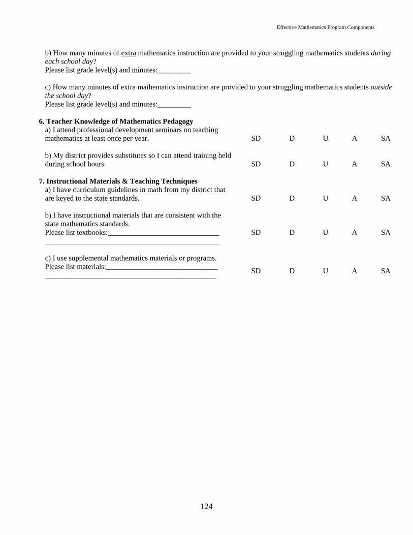
Effective Mathematics Program Components
124
b) How many minutes of extra mathematics instruction are provided to your struggling mathematics students during
each school day?
Please list grade level(s) and minutes:_________
c) How many minutes of extra mathematics instruction are provided to your struggling mathematics students outside
the school day?
Please list grade level(s) and minutes:_________
6. Teacher Knowledge of Mathematics Pedagogy a) I attend professional development seminars on teaching
mathematics at least once per year.
SD D U A SA
b) My district provides substitutes so I can attend training held
during school hours.
SD D U A SA
7. Instructional Materials & Teaching Techniques a) I have curriculum guidelines in math from my district that
are keyed to the state standards.
SD D U A SA
b) I have instructional materials that are consistent with the
state mathematics standards.
Please list textbooks:______________________________
_______________________________________________
SD D U A SA
c) I use supplemental mathematics materials or programs.
Please list materials:______________________________
______________________________________________
SD D U A SA

Effective Mathematics Program Components
125
8. Grouping for Math Instruction a) I work with students in small groups.
SD D U A SA
b) I regularly use flexible grouping, where I group and regroup
students based upon performance.
SD D U A SA
9. Professional Development a) Professional development that improves my teaching of
math is available to me.
SD D U A SA
b) The principal uses classroom observation to provide me with
feedback in teaching math.
SD D U A SA
c) The principal uses student math performance to provide me
with feedback in teaching math.
SD D U A SA
d) Mathematics teachers for my grade level have time to plan
together during the school day. SD D U A SA
SD = Strongly Disagree; D = Disagree; U = Uncertain; A = Agree; SA = Strongly Agree
9. Professional Development (continued) e) Instructional resource personnel provide math demonstration
lessons and in-class assistance at our school. SD D U A
SA
f) Instructional resource personnel help me improve student
performance.
SD D U A SA
g) There is someone available to help me when I have
questions about teaching math.
SD D U A SA
10. End of Year Analysis a) In addition to the state test, I give an end-of-year assessment
in mathematics.
SD D U A SA
b) I make regular modifications to my teaching based on
student performance. SD D U A SA
c) I use annual test results to modify my instruction. SD D U A SA
1) District Name _______________________________
2) School Name ________________________________
3) Number of years teaching experience_____
10) Undergraduate degree(s)
a) Major(s)_______________________________
b) Minor(s)_______________________________
4) Type of certification(s) _________________________
___________________________________________
11) Graduate Degree(s)
a) Masters________________________________

Effective Mathematics Program Components
126
5) Total Number of Math Classes You Teach _________
6) Total Number of Students You Teach _____________
b) Ed.D., Ph.D._____________________________
7) Number of Math Classes of Each Type:
___ ESL ___ Bilingual
___ Low-Performing ___ GT or Honors
___ Special Ed ___ Regular (All student
levels)
Other_____________________________________
8) Grade(s) you are presently teaching: ____________
9) Type of instruction:
a) ___ Self-Contained
b) ___ Departmentalized
c) ___Team Teacher
d) ___Resource Teacher
e) Other ___________________________________
12) Mathematics Courses Taken in College (Check
those that apply)
a) ___ College Algebra
b) ___ Geometry
c) ___ Finite Math
d) ___ Trigonometry
e) ___ Calculus
f ) ___ Probability and Statistics
g) ___ Logic
h) Were the above math classes taken in a
department of mathematics?
___ yes ___ no ___ mixed
Thank you for taking the time to complete this survey.

Effective Mathematics Program Components
127
Endnotes
1 Douglas Carnine, PhD, is a professor of education at the University of Oregon and director of the National Center to
Improve the Tools of Educators (NCITE).
2 The original version of component 6 was labeled ―Math Pedagogy‖.
3 The TAAS (Texas Assessment of Academic Skills) was the Texas statewide standardized test in place from 1994 to 2002.
It has now been superseded by the TAKS (Texas Assessment of Knowledge and Skills), based on more rigorous standards.
4 Toenjes & Garst (2000), p. ii.
5 Thomas, Warren + Associates (2003), pp. 10 – 15.
6 Under the Texas accountability system the focus was for schools and districts to achieve a minimum pass rate on the
state’s criterion referenced TAAS test. Ratings were based on the percentage of students meeting the minimum requirement
on the reading, writing, and mathematics tests. Under a system based on meeting year-to-year growth goals, the
measurement of growth depends upon the level achieved in each of the two years, current and most recent. Chance
variation in pass rates in each year, say an abnormally high rate followed the next year by an unusually (but not
improbable) low rate would often result in negative growth. This could occur even for schools or districts whose overall,
average achievement level is quite high. This instability in growth rates is more severe for small schools or those whose
sub-group populations are small in number, if sub-groups are independently assessed. See Kane, Staiger, & Geppert (2002)
for a succinct discussion of these effects.
7 The standard reference on hierarchical linear models, especially as applied to education research, is Bryk and
Raudenbush (1992). A paper with particular relevance to the problem of assessing schools, or in the current study of
assessing school districts, is Aitken and Longford (1986).
8 It is the estimate of u0j for each district j that is referred to as the modified mean residual (MMR) in the text herein. The
estimated variance of the uijs is denoted too above. As Bryk and Raudenbush observe, if the level 1 explanatory variable
EDij is removed from Equation I, then estimating Equations I – III is in effect performing a One-Way ANOVA with
Random Effects (Bryk and Raudenbush (1992), p. 17). In doing so, s2 is the estimate of the level 1 variance, too the estimate
of the level 2 variance. With this model, t00/(t00 + s2) represents the proportion of variance that is between the level 2 units.
In the current case, this would represent the proportion of total campus variation in reading scores attributable to inter-
district differences.
9Bryk and Raudenbush (1992), p. 125.
10
The major exception to this scale of 1 – 5 was in Component 5 (Increased and Effective Use of Instructional Time), where
the respondent was asked to indicate numbers of minutes of mathematics instruction provided both during the school day
and outside the school day. On the teachers’ questionnaire the wording for items pertaining to Component 5 elicited
responses that resulted in estimates of instructional time that could not be separated out by grade level. Rather than try to
estimate the grade level breakdown, this component was not used for teachers. As it turned out, the responses by principals
and district-level administrators did not prove to be an effective predictor of student performance either.
11
It was originally thought that it might be easier to combine the results for all three states using the percentile measure of
campus performance. As will be seen below, however, z-score transforms of the campus pass rates later seemed to be a
more straightforward solution to this problem.
12
See note10.
13
Students not having parents with at least a high school education or who must change schools frequently during the
academic year generally are thought to be more difficult to educate than students with more highly educated parents and
those whose living conditions are stable.

Effective Mathematics Program Components
128
14
See note 10.
15
The passing criterion represented by PPM for North Carolina is what that state terms ―Level III‖. Level II is defined as
―Students performing at this level consistently demonstrate mastery of grade level subject matter and skills and are well
prepared for the next grade level.‖
16
Evidence presented in Table 36 shows that there was considerably less variance in the response to the survey in North
Carolina than in California and Texas. Other things equal, this makes it less likely to account for variations in school or
district performance with these variables.
17
The Texas Assessment of Academic Skills (TAAS) was first administered to grades 3-8 and 10 in the spring of 1994. The
TAAS was a criterion referenced test designed to test the material in the statewide curriculum adopted by the State Board of
Education. Mathematics and reading were tested in all of the indicated grade levels each year, with writing tested only in
grades 4,8 and 10. In school year 2002-2003 the TAAS was replaced by a more demanding test, the TAKS. The
mathematics portion will be taken annually by all students in grades 3-11. Algebra will be included in the mandatory exit
exam (grade 11) for the first time. The test results for schools and school districts, by subject matter, for all years
beginning with 1994 are available for downloading from the Texas Education Agency’s Website
(http://www.tea.state.tx.us).
18
There is a real dilemma here. If the passing criterion is set low enough so that most students pass, then the school
average passing rates are less useful from the point of view of performing school-based analysis of the data for purposes of
trying to determine what procedures help improve average student performance. Increasing the passing threshold, though it
might help researchers, would result in school failure rates that might not be acceptable to the public. This would be
especially true if the result of failure is retention in grade or denial of graduation. While only a conjecture, it is also likely
that tougher passing standards would increase the apparent gap between different economic and social groups of students,
and might also affect the rate of improvement in passing rates following the imposition of an accountability system. States
imposing tougher standards might have more difficulty in meeting improvement goals as well as exhibiting high failure
rates.
19
In addition to concluding that the school district was the logical place to undertake reform, Stigler and Hiebert had some
specific reform in mind. Their comparisons of teaching practices in Japan, Germany, and the U.S. led them to conclude
that the reason no improvement has been seen in the effectiveness of U.S. teaching was because there was no mechanism
that allows U.S. teachers to learn from each other or even from their own mistakes. They described an institutionalized
system of teacher improvement among Japanese teachers that has existed for some fifty years. In the case of mathematics,
which was their focus, the teachers in each school undertake a study of one or more particular mathematics topics or
―lessons‖ each year. They spend a great deal of time and effort in meeting together to discus how the topic can be taught
more effectively, observe each other trying out their new approaches in the classroom, and finally write up the results so
teachers in other schools might benefit from their experience.
The observation by Stigler and Hiebert that U.S. teachers did not seem to improve very much with additional experience is
also reflected in the work of Liping Ma (1999). Ma emphasized that the Chinese teachers she interviewed in her study
comparing U.S. and Chinese elementary math teachers are given time and opportunity each day to meet and discuss their
classes. An important difference between U.S. and Chinese elementary teachers interviewed was that the Chinese teachers
specialized in teaching mathematics. The math teachers in each school typically shared a common office space, which
greatly facilitated frequent interaction. Ma found that, unlike their U.S. counterparts, more experienced Chinese teachers
exhibited more effective teaching skills than the less experienced teachers.