identify the i.v. and d.v. variables as you read the story: two researchers were talking shop over...

Identify the I.V. and D.V. variables as you read the story:

Two researchers were talking shop over coffee one morning. The topic was intensive early training in athletics. Both researchers were convinced that such training made the child less sociable as an adult, but one researcher went even further. “I think that really intensive training of young kids is ultimately detrimental to their performance in the sport. Why, I’ll bet that, among the top ten men’s single tennis players, those with intensive early training are not in the highest ranks.”

EDUCATIONAL STATISTICS EDU5950 WEEK14

Continued …“Well, I certainly wouldn’t go that far,” said the second researcher. “I think all that early intensive training is quite helpful.”

“Good. In fact, great. We disagree and we may be able to decide who is right. Let’s get the ground rules straight. For tennis players, how early is early and what is intensive?”

“Oh, I’d say early is starting by age 7 and intensive is playing every day for 2 or more hours.”


“That seem reasonable. Now, let’s see, our proportion is ‘excellent tennis players’ and these top ten will serve as our representative sample.”

Can you identify the I.V. and D.V.?

This is a new category of tests that can be used to analyze experiments in which the dependent variable is ranks.

This category is called nonparametric statistics.


Doing nonparametric statistics are also using the hypothesis-testing steps.

Write a paragraph about:- The null hypothesis- The alternative hypothesis- Gathering data- Using a sampling distribution- Making a decision about the null hypothesis- Telling a story that the data support


The different in the nonparametric statistics are those on sampling distribution of ranks.

How a sampling distribution based on ranks might be constructed?

Suppose you drew two samples of equal size (for example, N1 = N2 = 10) from the same population.

You then arranged all the scores from both samples into one overall ranking, from 1 to 20.


Because the samples are from the same population, the sum of the ranks of one group should be equal to the sum of the ranks of the second group.

After repeated sampling, all the sums could be arranged into a sampling distribution, which would allow you to determine the likelihood of any sum (if both samples come from the same population).

We’ll going to learn four new techniques – Mann-Whitney U, Wilcoxon matched-pairs signed-ranks test, Wilcoxon-Wilcox multiple-comparisons test, and Spearman rs (formely known as Spearman rho (ρ)).


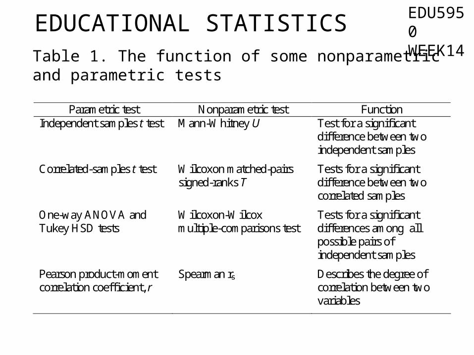
Table 1. The function of some nonparametric and parametric tests

EDUCATIONAL STATISTICS

Parametric test Nonparametric test Function Independent samples t test Mann-Whitney U Test for a significant

difference between two independent samples

Correlated-samples t test Wilcoxon matched-pairs signed-ranks T

Tests for a significant difference between two correlated samples

One-way ANOVA and Tukey HSD tests

Wilcoxon-Wilcox multiple-comparisons test

Tests for a significant differences among all possible pairs of independent samples

Pearson product-moment correlation coefficient, r

Spearman rs Describes the degree of correlation between two variables

EDU5950 WEEK14

The Mann-Whitney U test

Nonparametric test for data from an independent-samples design.

Produces a statistics, U – that is evaluated by consulting the sampling distribution of U.

When sample sizes are relatively small, critical value of U can be found in Table H.


Use Table H if N1 = 20 or less and N2 = 20 or less.

If the number of scores in one of the samples is greater than 20, the statistic U is distributed approximately as a normal.

In this case, a z score is calculated, and the values of ±1.96 and ±2.58 are used as critical values for α = .05 and α = .01

Table 2 illustrate the intensive early training of the top ten male singles tennis players.


Table 2

ΣRyes = 4 + 6 + 8 + 9 = 27

ΣRno = 1 + 2 + 3 + 5 + 7 + 10


Players Rank Intensive early

training Y.O. 1 No

U.E. 2 No

X.P. 3 No

E.C. 3 Yes

T.E. 5 No

D.W. 6 Yes

O.R. 7 No

D.S. 8 Yes

H.E. 9 Yes

R.E. 10 No

EDU5950 WEEK14

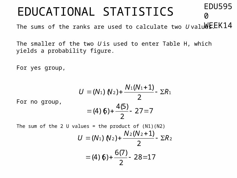
The sums of the ranks are used to calculate two U values.

The smaller of the two U is used to enter Table H, which yields a probability figure.

For yes group,

For no group,

The sum of the 2 U values = the product of (N1)(N2)


7272

)5(4)6)(4(

2

)1())(( 1

1121

RNN

NNU

17282

)7(6)6)(4(

2

)1())(( 2

2221

RNN

NNU

EDU5950 WEEK14

Refer to Table H,

the lightface type gives a critical values for α levels of .01 for a one tailed test and .02 for a two tailed test.

the boldface type are critical values for α = .005 for a one-tailed test and α = .01 for a two-tailed test.

In similar way, the other page gives larger α values for both one- and two-tailed tests.


Back to our problem earlier, test the U = 7 value from the tennis data.

From Table H, by looking for critical value of U for a two-tailed test with α = .05. The critical value is 2.

Because the obtained value of U is 7, you must retain the null hypothesis and concluded that there is no evidence from the sample that the distribution of players trained early and intensively is significantly different from the distribution of those without such training.


The Wilcoxon Matched-Pairs Signed-Ranks T Test

Is appropriate for testing difference between two correlated samples.

The result of a Wilcoxon matched-pairs signed-ranks test is a T value – interpreted using Table J.

Based on data in Table 3, the following steps lead to a T value for a Wilcoxon matched-pairs signed-ranks T:


Find a difference, D, for every pair of scores. The order of subtraction doesn’t matter, but it must be the same for every pair.

Using the absolute value for each difference, rank the differences.

The rank of 1 is given to the smallest difference, 2 goes to the next smallest, and so on.

Attach to each rank the sign of its difference. Thus, if a difference produces a negative value, the rank for that pair is negative.


Sum the positive ranks and sum the negative ranks.

T is the smaller of the absolute values of the two sums.

Table 3

Σ(positive ranks) = 6Σ(negative ranks) = -4 T = 4


Pair Variable1 Variable2 D Rank Signed

rank A 16 24 -8 3 -3

B 14 17 -3 1 -1

C 23 18 5 2 2

D 23 9 14 4 4

EDU5950 WEEK14

Table J shows the critical values for both one- and two-tailed tests for several α levels.

To enter the table, use N, the number of pairs of subjects.

Reject H0 when the obtained T is equal to or less than the critical in the table.

Note: Ties among the D scores – each tied score is assigned the mean of the ranks that would have assigned if there had been no ties


The Wilcoxon-Wilcox Multiple-Comparisons TestAllows to compare all possible pairs of treatments.

This is like running several Mann-Whitney tests on each pair of treatments.

This test requires independent samples.

The following steps walk us through this test:

Ordering the scores from the K treatments into one overall ranking.


Within each sample, add the ranks, which gives a ΣR for each sample.

For each pair of treatments, subtract one ΣR from the other, which gives a difference.

Finally, compare the absolute size of the difference to a critical value in Table K.

This test can be used only when the N’s for all groups are equal.


The data in Table 4 represent the results of an experiment conducted on a solar collector.

Ranks are given to each temperature, ignoring the group the temperature is in.

The ranks of all those in a group are summed, producing ΣR values that range from 20 to 84 for flow rates of 14 to 17 gallons per hour.


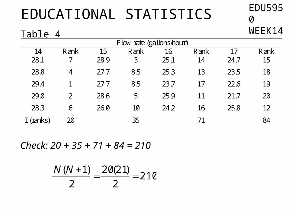
Table 4

Check: 20 + 35 + 71 + 84 = 210


Flow rate (gallons/hour) 14 Rank 15 Rank 16 Rank 17 Rank

28.1 7 28.9 3 25.1 14 24.7 15

28.8 4 27.7 8.5 25.3 13 23.5 18

29.4 1 27.7 8.5 23.7 17 22.6 19

29.0 2 28.6 5 25.9 11 21.7 20

28.3 6 26.0 10 24.2 16 25.8 12

Σ(ranks) 20 35 71 84

2102

)21(20

2

)1(

NN

EDU5950 WEEK14

The next step is to make pairwise comparisons.

With four group, six pairwise comparisons are possible:The rate of 14 gallons per hour can be paired with 15, 16, and 17;The rate of 15 can be paired with 16 and 17; andThe rate of 16 can be paired with 17.

For each pair, a difference in the sum of ranks is found and the absolute value of that difference is compared with the critical value in Table K.


The upper half of Table K has critical value for α = .05; the lower half has values for α = .01.

For the experiment in Table 4, where K = 4 and N = 5, the critical values are 48.1 (α = .05) and 58.2 (α = .01).

To reject H0, a difference in rank sums must be equal to or greater than the critical values.

It is convenient to arrange the differences in rank sums into a matrix summary table as in Table 5.


Table 5


14 15 16

15 15

16 51 36

17 64 49 13

EDU5950 WEEK14

The Spearman rs (formely known as Spearman ρ (Rho))

Spearman rs is a special case of the Pearson product-moment correlation coefficient and is most often used when the number of pairs of scores is small (less than 20).

Spearman’s name is attached to the coefficient that is used to show the degree of correlation between two sets of ranked data.

The formula for rs is,

Where; D = difference in ranks of a pair of scores

N = number of pairs of scores


)1(

6 1

NN

Drs

EDU5950 WEEK14

Let say we have an actual data for female tennis player.

What is the progression in women’s professional tennis?

Do they work their way up through the ranks, advancing their ranking year by year?

Or do the younger player flash to the top and then gradually lose their ranking year by year?

An rs might lend support to one of these hypotheses.


If the rank of 1 is assigned to the oldest player, a positive rs means that the older the player, the higher her rank (support first hypothesis).

A negative rs means that the older the player, the lower her rank (supporting the second hypothesis).

A zero rs means no relationship between age and rank.

How to testing the significance of rs?


Table 6 shows the ten top ranked women tennis players for 1998, their age as a rank score among the ten, and rs of -.20.


Player

Rank in tennis

Rank in age

D

D2

Davenport (USA) 1 7 -6 36 Hingis (Switzerland) 2 10 -8 64 Novotna (Czech Republic) 3 2 1 1 Sanchez-Vicario (Spain) 4 3 1 1 Williams (USA) 5 9 -4 16 Seles (USA) 6 5 1 1 Pierce (France) 7 6 1 1 Tauziat (France) 8 1 7 49 Martinez (Spain) 9 4 5 25 Schnyder (Switzerland) 10 8 2 4 Σ = 198

20.20.11)99(10

)198(61

)1 (

6 1

NN

Drs

EDU5950 WEEK14

For a sample rs, you can test the null hypothesis that the population correlation coefficient is .00.

That is, a sampling distribution of rs values taken from a population in which the true correlation is zero will show you the probability of various rs‘s.

If the probability for your sample rs is small, reject the null hypothesis and conclude that the relationship in the population that rs came from is not zero.

Table L gives critical values for rs for the .05 and .01 levels of significance (when the number of pairs is 16 or fewer).


Reject the hypothesis that the population correlation coefficient is zero if the obtained rs is equal to or greater than the tabled value.

Refer to Table 1, rs = -.20 based on ten pairs. Table L shows that a correlation of .648 (either positive or negative) is required for significance at the .05 level.

Thus, a correlation of -.20 is not statistically significant.
