identification of the lldpe constitutive material model
TRANSCRIPT
polymers
Article
Identification of the LLDPE Constitutive Material Model forEnergy Absorption in Impact Applications
Ludek Hyncík 1,* , Petra Kochová 2 , Jan Špicka 1 , Tomasz Bonkowski 1 , Robert Cimrman 1 ,Sandra Kanáková 2 , Radek Kottner 2 and Miloslav Pašek 3
�����������������
Citation: Hyncík, L.; Kochová, P.;
Špicka, J.; Bonkowski, T.; Cimrman,
R.; Kanáková, S.; Kottner, R.; Pašek,
M. Identification of the LLDPE
Constitutive Material Model for
Energy Absorption in Impact
Applications. Polymers 2021, 13, 1537.
https://doi.org/ 10.3390/
polym13101537
Academic Editor: Mauro Zarrelli
Received: 23 March 2021
Accepted: 6 May 2021
Published: 11 May 2021
Publisher’s Note: MDPI stays neutral
with regard to jurisdictional claims in
published maps and institutional affil-
iations.
Copyright: © 2021 by the authors.
Licensee MDPI, Basel, Switzerland.
This article is an open access article
distributed under the terms and
conditions of the Creative Commons
Attribution (CC BY) license (https://
creativecommons.org/licenses/by/
4.0/).
1 New Technologies—Research Centre, University of West Bohemia, 301 00 Plzen, Czech Republic;[email protected] (J.Š.); [email protected] (T.B.); [email protected] (R.C.)
2 Faculty of Applied Sciences, University of West Bohemia, 301 00 Plzen, Czech Republic;[email protected] (P.K.); [email protected] (S.K.); [email protected] (R.K.)
3 MECAS ESI s.r.o., Brojova 2113, 326 00 Plzen, Czech Republic; [email protected]* Correspondence: [email protected]
Abstract: Current industrial trends bring new challenges in energy absorbing systems. Polymermaterials as the traditional packaging materials seem to be promising due to their low weight,structure, and production price. Based on the review, the linear low-density polyethylene (LLDPE)material was identified as the most promising material for absorbing impact energy. The currentpaper addresses the identification of the material parameters and the development of a constitutivematerial model to be used in future designs by virtual prototyping. The paper deals with theexperimental measurement of the stress-strain relations of linear low-density polyethylene understatic and dynamic loading. The quasi-static measurement was realized in two perpendicularprincipal directions and was supplemented by a test measurement in the 45◦ direction, i.e., exactlybetween the principal directions. The quasi-static stress-strain curves were analyzed as an initialstep for dynamic strain rate-dependent material behavior. The dynamic response was tested in adrop tower using a spherical impactor hitting a flat material multi-layered specimen at two differentenergy levels. The strain rate-dependent material model was identified by optimizing the staticmaterial response obtained in the dynamic experiments. The material model was validated by thevirtual reconstruction of the experiments and by comparing the numerical results to the experimentalones.
Keywords: LLDPE; quasi-static and dynamic experimental tests; impact energy absorption; materialparameter identification; constitutive material model; validation; simulation
1. Introduction
Thin-layered polymer materials are traditionally used for packaging goods to protectthem during transportation. Therefore, the major desired properties relate to thickness,density (which relates to weight), strength, elongation, puncture resistance, and stretchinglevel; see Table 1. On the other hand, preliminary experimental tests also show the goodperformance of such materials in energy absorption.
Current trends in the automotive industry regarding future mobility bring new chal-lenges for energy-absorbing safety systems. Non-traditional seating configurations inautonomous vehicles and complex crash scenarios including multi-directional loadingare to be considered hand-in-hand with advanced materials for energy absorption. Thestudy [1] used a numerical simulation approach to assess the newly patented safety system(see Figure 1) [2]. The system is based on two layers of a multi-layered membrane injectedfrom the roof between the windshieldand the front seats, catching the driver and thepassenger during an accident in a similar manner as an airbag performs. The advantage ofthe approach over the airbag is the simple implementation for multi-directional impactloading and addressing the out-of-position seating issue.
Polymers 2021, 13, 1537. https://doi.org/10.3390/polym13101537 https://www.mdpi.com/journal/polymers
Polymers 2021, 13, 1537 2 of 25
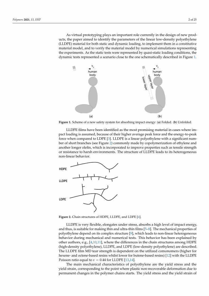
As virtual prototyping plays an important role currently in the design of new prod-ucts, the paper aimed to identify the parameters of the linear low-density polyethylene(LLDPE) material for both static and dynamic loading, to implement them in a constitutivematerial model, and to verify the material model by numerical simulations representingthe experiments. As the static tests were represented by quasi-static loading conditions, thedynamic tests represented a scenario close to the one schematically described in Figure 1.
v0
humanbody
(a)
v0
lower layer
upper layer
humanbody
(b)
Figure 1. Scheme of a new safety system for absorbing impact energy: (a) Folded. (b) Unfolded.
LLDPE films have been identified as the most promising material in cases where im-pact loading is assumed, because of their higher average peak force and the energy-to-peakforce when compared to LDPE [3]. LLDPE is a linear polyethylene with a significant num-ber of short branches (see Figure 2) commonly made by copolymerization of ethylene andanother longer olefin, which is incorporated to improve properties such as tensile strengthor resistance to harsh environments. The structure of LLDPE leads to its heterogeneousnon-linear behavior.
Figure 2. Chain structures of HDPE, LLDPE, and LDPE [4].
LLDPE is very flexible, elongates under stress, absorbs a high level of impact energy,and thus, is suitable for making thin and ultra-thin films [5–8]. The mechanical properties ofpolyethylene depend on its complex structure [9], which leads to non-linear heterogeneousbehavior during mechanical and numerical tests. This behavior has been explained byother authors, e.g., [4,10,11], where the differences in the chain structures among HDPE(high-density polyethylene), LLDPE, and LDPE (low-density polyethylene) are described.The LLDPE film MD tear strength is dependent on the utilized comonomers (higher forhexene- and octene-based resins whilst lower for butene-based resins) [12] with the LLDPEPoisson ratio equal to ν = 0.44 for LLDPE [13,14].
The main mechanical characteristics of polyethylene are the yield stress and theyield strain, corresponding to the point where plastic non-recoverable deformation due topermanent changes in the polymer chains starts. The yield stress and the yield strain of
Polymers 2021, 13, 1537 3 of 25
LLDPE depend on the temperature and the strain rate [5,6,15]. The yield stress increaseswhile the yield strain decreases with rising strain rate [9]. The double yield point is alsomentioned in the literature [16]. The relation between yield stress, temperature, andstrain rate can be described by constitutive laws [5,6,9,17], and the temperature-dependentmechanical properties of thin-layered materials have been addressed [18]. Upon comparingLDPE, LLDPE, and HDPE, LLDPE showed greater rate sensitivity than the other twomaterials under both static and dynamic regions of a compression test [9].
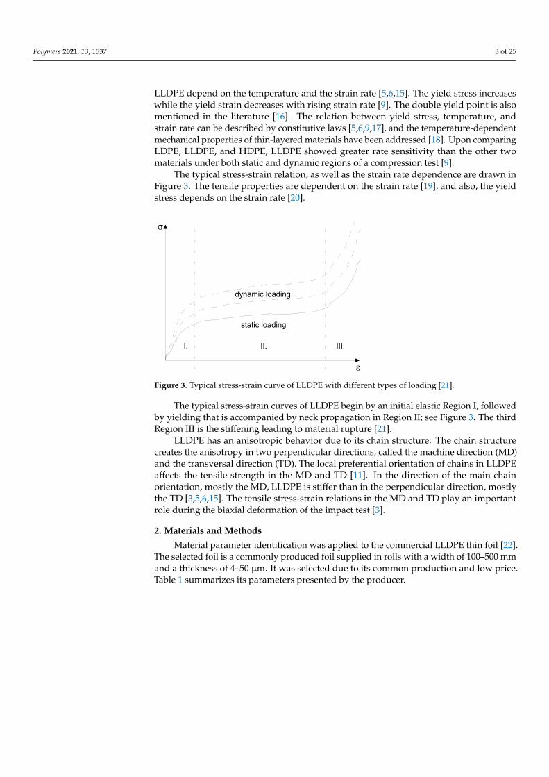
The typical stress-strain relation, as well as the strain rate dependence are drawn inFigure 3. The tensile properties are dependent on the strain rate [19], and also, the yieldstress depends on the strain rate [20].
static loading
ε
I. II. III.
dynamic loading
σ
Figure 3. Typical stress-strain curve of LLDPE with different types of loading [21].
The typical stress-strain curves of LLDPE begin by an initial elastic Region I, followedby yielding that is accompanied by neck propagation in Region II; see Figure 3. The thirdRegion III is the stiffening leading to material rupture [21].
LLDPE has an anisotropic behavior due to its chain structure. The chain structurecreates the anisotropy in two perpendicular directions, called the machine direction (MD)and the transversal direction (TD). The local preferential orientation of chains in LLDPEaffects the tensile strength in the MD and TD [11]. In the direction of the main chainorientation, mostly the MD, LLDPE is stiffer than in the perpendicular direction, mostlythe TD [3,5,6,15]. The tensile stress-strain relations in the MD and TD play an importantrole during the biaxial deformation of the impact test [3].
2. Materials and Methods
Material parameter identification was applied to the commercial LLDPE thin foil [22].The selected foil is a commonly produced foil supplied in rolls with a width of 100–500 mmand a thickness of 4–50 µm. It was selected due to its common production and low price.Table 1 summarizes its parameters presented by the producer.
Polymers 2021, 13, 1537 4 of 25
Table 1. LLDPE properties [22].
Physical Properties Unit Tolerance ± Value Testing Method
Thickness µm 2 12 Thickness gaugeWidth mm 5 500 Measuring tapeLength - 5 High-speed encoderDensity g/cm3 - 0.91–0.92 ASTM D-1505 [23]
Mechanical Properties Unit Tolerance ± Value Testing Method
Tensile strength MD MPa
10
29.2
ASTM D-882 [23]Tensile strength TD 14.1Break elongation MD % 245Break elongation TD 540
Dart drop g 40 ASTM D-1709 [23]Puncture kg 1.7 High-light testerStretching level - - 110
2.1. Quasi-Static Loading
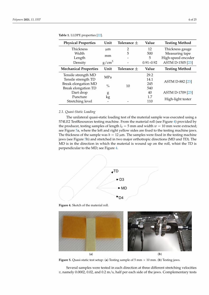
The unilateral quasi-static loading test of the material sample was executed using a574LE2 TestResources testing machine. From the material roll (see Figure 4) provided bythe producer, testing samples of length l0 = 5 mm and width w = 10 mm were extracted;see Figure 5a, where the left and right yellow sides are fixed to the testing machine jaws.The thickness of the sample was h = 12 µm. The samples were fixed in the testing machinejaws (see Figure 5b) and stretched in two major orthotropic directions (MD and TD). TheMD is in the direction in which the material is wound up on the roll, whist the TD isperpendicular to the MD; see Figure 4.
MD
D3
TD
D4
Figure 4. Sketch of the material roll.
(a) (b)
Figure 5. Quasi-static test setup: (a) Testing sample of 5 mm × 10 mm. (b) Testing jaws.
Several samples were tested in each direction at three different stretching velocitiesv, namely 0.0002, 0.02, and 0.2 m/s, half per each side of the jaws. Complementary tests
Polymers 2021, 13, 1537 5 of 25
in the directions between the MD and TD (labeled as D3 and D4; see Figure 4) weredone to check the influence of fiber direction on the material behavior in the skewed (45◦)direction. Table 2 summarizes all the quasi-static tests. N = 6 samples were measured ineach direction for each velocity except v = 0.2 m/s, where D4 did not need to be measured.As the additional measurements in D3 showed a consistent skewed behavior in all threevelocities and the additional measurement in D4 (which is D3 just rotated around 90◦)confirmed the skewed behavior for the first two velocities, the measurement for the lastvelocity was performed only in MD, TD, and D3. The particular test finished when thesample ruptured.
During the sample stretching, force F versus displacement d was recorded. Based onthe sample size with the sample initial length l0 and initial cross-sectional area A0 = hw,the engineering stress σ versus engineering strain ε curves were calculated as:
σ =F
A0, ε =
dl0
. (1)
The constant Young modulus E was also identified as the slope of the initial elasticregion as:
σ =F
A0= E
dl0
⇒ E =Fl0dA0
. (2)
Table 2. Quasi-static tests matrix.
Stretching Velocity v (m/s) Direction Number of Samples N
0.0002
MD 6TD 6D3 6D4 6
0.02
MD 6TD 6D3 6D4 6
0.2MD 6TD 6D3 6
Fulfilling the aim of this study, the quasi-static tests were reproduced by the numericalsimulations. The simulation was realized in Virtual Performance Solution (VPS by ESIGroup), Version 2020. Following the structure of LLDPE in Figure 3 (2 mutually perpen-dicular sets of fibers), the material model 151 Fabric Membrane Element with NonlinearFibers [24] from the ESI constitutive material model database was proposed. Accord-ing to membrane theory, the resultant stress curves were calculated by multiplying theengineering stress by the membrane thickness as:
σh = σh (3)
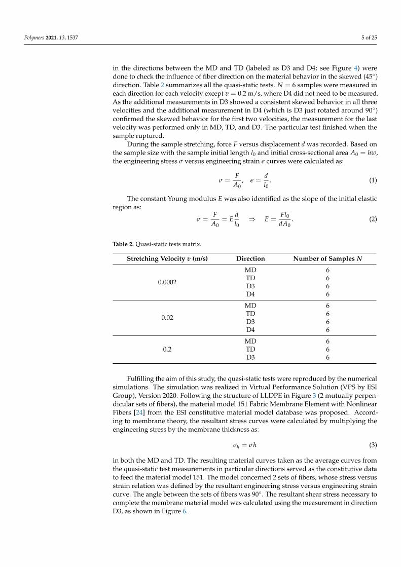
in both the MD and TD. The resulting material curves taken as the average curves fromthe quasi-static test measurements in particular directions served as the constitutive datato feed the material model 151. The model concerned 2 sets of fibers, whose stress versusstrain relation was defined by the resultant engineering stress versus engineering straincurve. The angle between the sets of fibers was 90◦. The resultant shear stress necessary tocomplete the membrane material model was calculated using the measurement in directionD3, as shown in Figure 6.
Polymers 2021, 13, 1537 6 of 25
TD
MD
D3
F3Q
γ
L
Qψ
L
Figure 6. Evaluating the resultant shear stress.
Supposing a square sample, the shear force Q and shear angle γ were calculatedthrough the following formulas.
Q =F3
2 cos ψ2
, (4)
where the shear angle:
γ =π
2− ψ (5)
was calculated based on the deformed sample angle ψ as:
cosψ
2=
√2L + d2L
, (6)
where L is the side of the square sample, d is the displacement in direction D3, and F3 isthe force recorded in direction D3. Therefore, the shear stress can be calculated as:
τ =QLh
(7)
and the resultant shear stress is:τh = τh =
QL
. (8)
The thickness of the material was h = 12 µm, as defined by the producer [22]. Inaddition to the stress-strain constitutive relations, the chosen material model [24] requiresalso the amount of energy absorption. The energy absorption was calculated from thedynamic experimental measurements, and other numerical parameters feeding the materialmodel were used as proposed by the VPS manual [24].
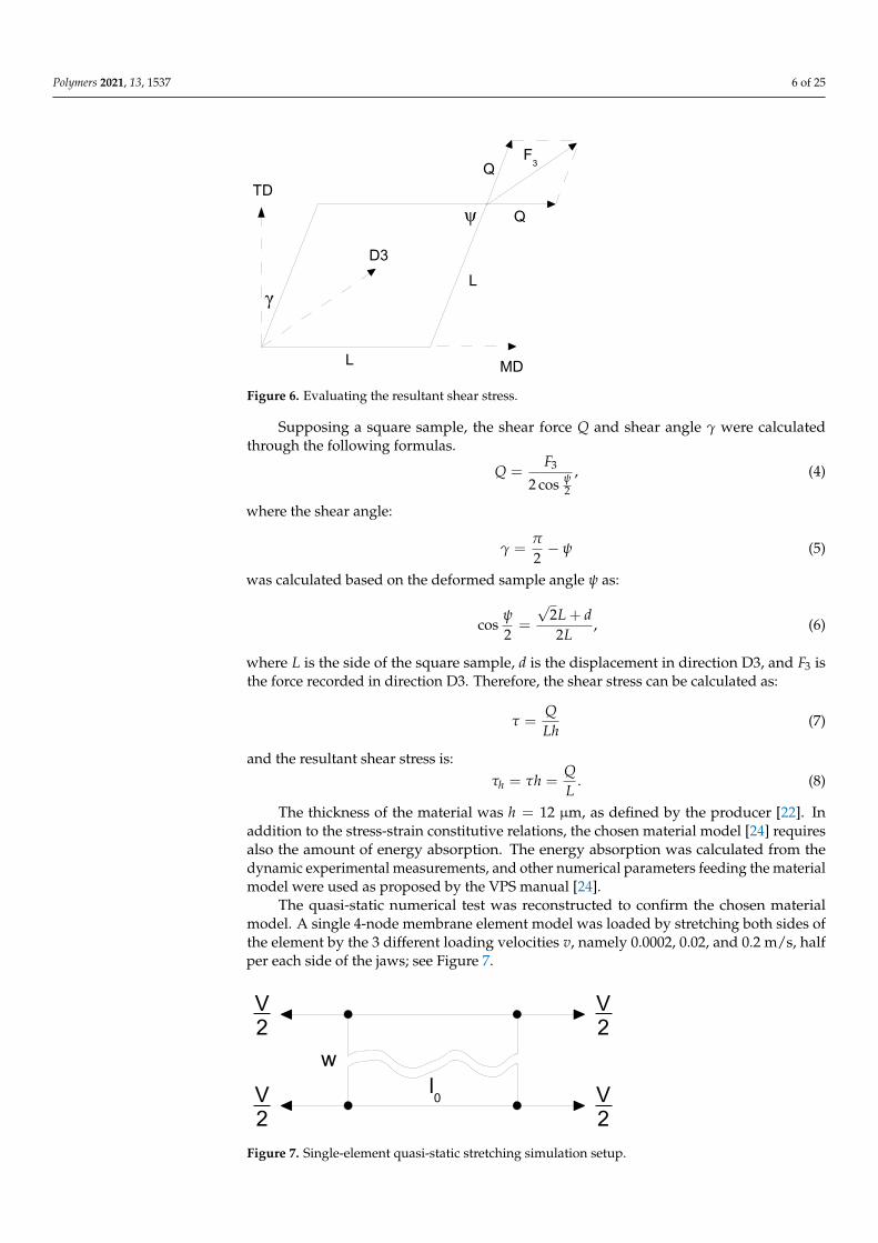
The quasi-static numerical test was reconstructed to confirm the chosen materialmodel. A single 4-node membrane element model was loaded by stretching both sides ofthe element by the 3 different loading velocities v, namely 0.0002, 0.02, and 0.2 m/s, halfper each side of the jaws; see Figure 7.
V2
V2
V2
V2
l0
w
Figure 7. Single-element quasi-static stretching simulation setup.
Polymers 2021, 13, 1537 7 of 25
The element section force leading to the resultant stress was recorded during thesimulation to be compared to the experimental data.
2.2. Dynamic Loading
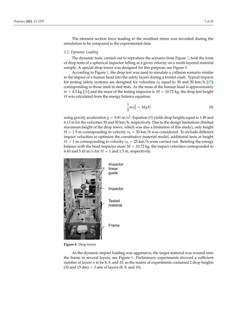
The dynamic tests, carried out to reproduce the scenario from Figure 1, took the formof drop tests of a spherical impactor falling at a given velocity on a multi-layered materialsample. A special drop tower was designed for this purpose; see Figure 8.
According to Figure 1, the drop test was used to simulate a collision scenario similarto the impact of a human head into the safety layers during a frontal crash. Typical impactsfor testing safety systems are designed for velocities v0 equal to 30 and 50 km/h [25],corresponding to those used in sled tests. As the mass of the human head is approximatelym = 4.5 kg [26] and the mass of the testing impactor is M = 10.72 kg, the drop test heightH was calculated from the energy balance equation:
12
mv20 = MgH (9)
using gravity acceleration g = 9.81 m/s2. Equation (9) yields drop heights equal to 1.49 and4.13 m for the velocities 30 and 50 km/h, respectively. Due to the design limitations (limitedmaximum height of the drop tower, which was also a limitation of this study), only heightH = 1.5 m corresponding to velocity v0 = 30 km/h was considered. To include differentimpact velocities to optimize the constitutive material model, additional tests at heightH = 1 m corresponding to velocity v0 = 25 km/h were carried out. Relating the energybalance with the head impactor mass M = 10.72 kg, the impact velocities corresponded to4.43 and 5.43 m/s for H = 1 and 1.5 m, respectively.
Impactorlinearguide
Impactor
Testedmaterial
Frame
MD
TD
Figure 8. Drop tower.
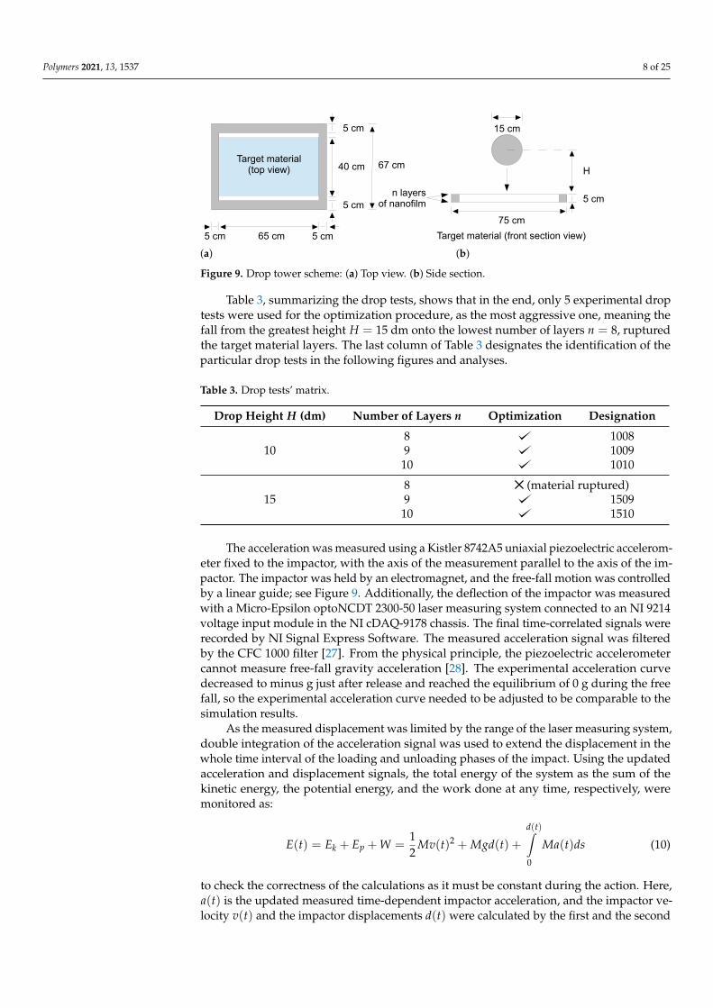
As the dynamic impact loading was aggressive, the target material was wound ontothe frame in several layers; see Figure 9. Preliminary experiments showed a sufficientnumber of layers n to be 8, 9, and 10, so the matrix of experiments contained 2 drop heights(10 and 15 dm) × 3 sets of layers (8, 9, and 10).
Polymers 2021, 13, 1537 8 of 25
40 cm
5 cm
Target material(top view) 67 cm
5 cm
65 cm5 cm 5 cm
n layersof nanofilm 5 cm
75 cm
15 cm
H
Target material (front section view)
(a) (b)
Figure 9. Drop tower scheme: (a) Top view. (b) Side section.
Table 3, summarizing the drop tests, shows that in the end, only 5 experimental droptests were used for the optimization procedure, as the most aggressive one, meaning thefall from the greatest height H = 15 dm onto the lowest number of layers n = 8, rupturedthe target material layers. The last column of Table 3 designates the identification of theparticular drop tests in the following figures and analyses.
Table 3. Drop tests’ matrix.
Drop Height H (dm) Number of Layers n Optimization Designation
108 10089 100910 1010
158 (material ruptured)9 150910 1510
The acceleration was measured using a Kistler 8742A5 uniaxial piezoelectric accelerom-eter fixed to the impactor, with the axis of the measurement parallel to the axis of the im-pactor. The impactor was held by an electromagnet, and the free-fall motion was controlledby a linear guide; see Figure 9. Additionally, the deflection of the impactor was measuredwith a Micro-Epsilon optoNCDT 2300-50 laser measuring system connected to an NI 9214voltage input module in the NI cDAQ-9178 chassis. The final time-correlated signals wererecorded by NI Signal Express Software. The measured acceleration signal was filteredby the CFC 1000 filter [27]. From the physical principle, the piezoelectric accelerometercannot measure free-fall gravity acceleration [28]. The experimental acceleration curvedecreased to minus g just after release and reached the equilibrium of 0 g during the freefall, so the experimental acceleration curve needed to be adjusted to be comparable to thesimulation results.
As the measured displacement was limited by the range of the laser measuring system,double integration of the acceleration signal was used to extend the displacement in thewhole time interval of the loading and unloading phases of the impact. Using the updatedacceleration and displacement signals, the total energy of the system as the sum of thekinetic energy, the potential energy, and the work done at any time, respectively, weremonitored as:
E(t) = Ek + Ep + W =12
Mv(t)2 + Mgd(t) +
d(t)∫0
Ma(t)ds (10)
to check the correctness of the calculations as it must be constant during the action. Here,a(t) is the updated measured time-dependent impactor acceleration, and the impactor ve-locity v(t) and the impactor displacements d(t) were calculated by the first and the second
Polymers 2021, 13, 1537 9 of 25
integration, respectively, of the acceleration signal a(t). The gravity acceleration g wassubtracted from the impactor acceleration to subtract the work done by the potential energy.
Marking Ekp(t) = Ek(t) + Ep(t) as the sum of the kinetic energy and potential energyat any time, the energy absorption was calculated as the energy loss at any time:
D = 1− ∆Eu
∆El, (11)
where ∆El = max Ekp(t) −min Ekp(t)|loading is the difference between the maxima ofthe sum of the kinetic energy and potential energy during the loading phase and ∆Eu =max Ekp(t)−min Ekp(t)|unloading is the energy difference between the maxima of the sumof the kinetic energy and potential energy during the unloading phase, where the restingenergy is absorbed by the material work in order to have the constant total energy E(t)from Equation (10).
2.3. Identification of Dynamic Material Parameters
As the material properties of LLDPE are strain rate dependent [21], the constitutivematerial curves achieved by the quasi-static experimental measurements were used asthe initial optimization step for the optimization of the dynamic material parameters.The optimization was done using the numerical simulation reproducing the drop testexperiment. The strain rate-dependent curves from the first optimization (H = 10 dm andn = 8 layers) were used as the initial curves for the other optimization runs to speed upthe optimization process.
The standard MATLAB function fminsearch was adopted to optimize the valuesfor the stiffness and the yield stress in the two directions MD and TD towards the ex-pected values. According to Figure 3, the stiffness of Region I and the yield stress wereoptimized. For the optimization purposes, Region I was divided into 2 strain intervalsε ∈ [0, εMD
y1 ] ∪ (εMDy1 , εMD
y2 ] for the MD response and ε ∈ [0, εTDy1 ] ∪ (εTD
y1 , εTDy2 ] for the TD
response. The corresponding stress interval was composed as σ ∈ [0, σMDy1 ] ∪ (σMD
y1 , σMDy2 ]
for the MD response and σ ∈ [0, σTDy1 ] ∪ (σTD
y1 , σTDy2 ] for the TD response so that the yield
points [εMDy1 , σMD
y1 ] and [εMDy2 , σMD
y2 ] in the MD response and [εTDy1 , σTD
y1 ] and [εTDy2 , σTD
y2 ] in theTD response were introduced. Addressing the resultant stress in Equation (3), the MD andTD curves in Region I were updated as:
σMDh := σMD
h (ε, k1, ke, ky) = kyσMDh
( ε
k
), k =
{k1ke ∀ε ∈ [0, εMD
y1 ]
ke ∀ε ∈ (εMDy1 , εMD
y2 ](12)
σTDh := σTD
h (ε, k1, ke, ky) = kyσTDh
( ε
k
), k =
{k1ke ∀ε ∈ [0, εTD
y1 ]
ke ∀ε ∈ (εTDy1 , εTD
y2 ](13)
by multiplying by dimensionless coefficients 1k1ke
, 1ke
, and ky during the optimizationprocess. The coefficient k scales with the strain in Region I, in particular k1ke until the firstyield point is reached and ke further between both yield points. The coefficient ky scaleswith the resultant stress. Such a parametric representation of the constitutive curves wasproposed based on the preliminary numerical tests, which also confirmed the use of thesame multipliers k1, ke, and ky for both Equations (12) and (13) to hold the physical meaningof the optimized constitutive curves. For the independent sets of coefficients for the curvesin the MD and TD, the optimizer strengthened the MD, whilst the TD was completelysuppressed. Therefore, both sets of coefficients needed to be constrained together. Theoptimization process was run in a loop controlled by a MATLAB script updating the

Polymers 2021, 13, 1537 10 of 25
constitutive material curves in the MD and TD according to Equations (12) and (13). Thecost function in the optimization measured the relative acceleration error Ea defined as:
Ea =‖as(t)− ae(t)‖‖ae(t)‖
∣∣∣t∈[t1,tm ]
, (14)
where ae(t) is the time-dependent acceleration signal measured from the experiment, as(t)is the time-dependent acceleration response calculated by the numerical simulation, and tis the time in the error calculation interval [t1, tm]. As well as the experimental accelerationsignal, the calculated acceleration signal was also filtered by the CFC 1000 filter [27].Figure 10 shows the simulation setup for the optimization runs. The initial pre-strain of thematerial wound on the frame was estimated based on preliminary numerical simulationsto be 10%, i.e., ε0 = 0.1 in the MD. The displacement error Ed was calculated similarly tothe acceleration error as:
Ed =‖ds(t)− de(t)‖‖de(t)‖
∣∣∣t∈[t1,tm ]
, (15)
where de(t) is the time-dependent displacement signal obtained by the double integrationof the acceleration signal and ds(y) is the time-dependent displacement response calculatedby the numerical simulation.
Figure 10. Drop test simulation setup.
The interval for calculating the acceleration error in Equation (14) was limited to theloading phase for t ∈ [t1, tm] because the constitutive material model was developed forthe energy absorption during the stretching. Moreover, expanding the time interval to theunloading phase negatively influenced the optimized curve fit during the loading phase.The discretization of the time interval as t ∈ {t1, . . . , ti, . . . , tm} led to the cost function:
f =
m∑
i=1[as(ti)− ae(ti)]
m∑
i=1ae(ti)
, i ∈ {1, 2, . . . , m}, (16)
where ae(ti) is the measured acceleration signal sampled at discrete times ti and as(ti) is thecalculated acceleration signal based on the constitutive curves from Equations (12) and (13).Therefore, the cost function had the form:
f = f (k1, ke, ky), (17)
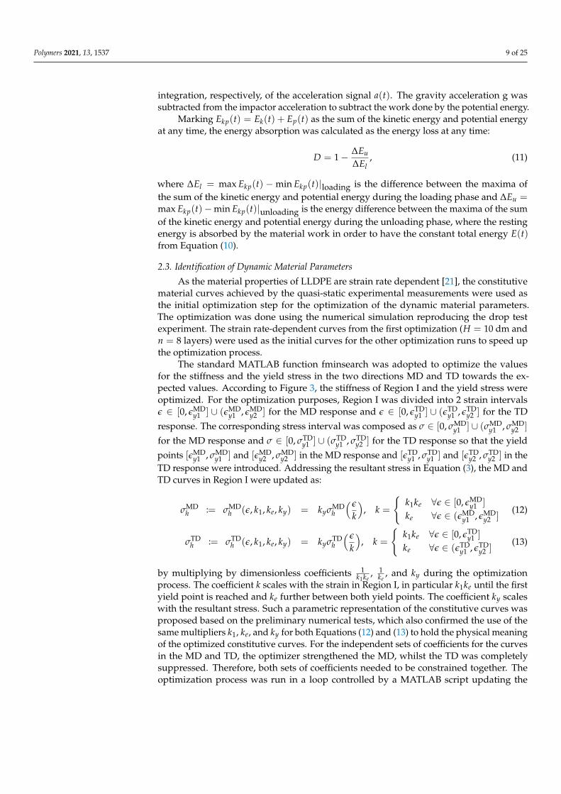
depending on three coefficients, k1, ke, and ky, whose values were updated during theoptimization process by the standard MATLAB function fminsearch. The update of thequasi-static constitutive curves is illustrated in Figure 11. Note that evaluating the three-parameter function f in Equation (17) involved running a finite element simulation of thedrop test to get as(ti). Considering that ε and σh represent the strain and the resultantstress, respectively, the optimization loop was:
Polymers 2021, 13, 1537 11 of 25
1. Update both the MD and TD curves according to Equations (12) and (13):
(a) ∀ε ∈ [0, εy1 ] update the stiffness by changing the slopes of the curves usingε := 1
k1keε;
(b) ∀ε ∈ (εy1 , εy2 ] update the stiffness by changing the slopes of the curves usingε := 1
ke(ε− εy1) + εy1 ;
(c) ∀ε ∈ [0, εy2 ] update the resultant stress as σh := kyσh;(d) ∀ε > εy2 connect the parts of the curves in Regions II and III to the second
yield point using ε := ε + ∆εy2 and σh := σh + ∆σhy2 where [∆εy2 , ∆σhy2] is the
shift of the second yield point;
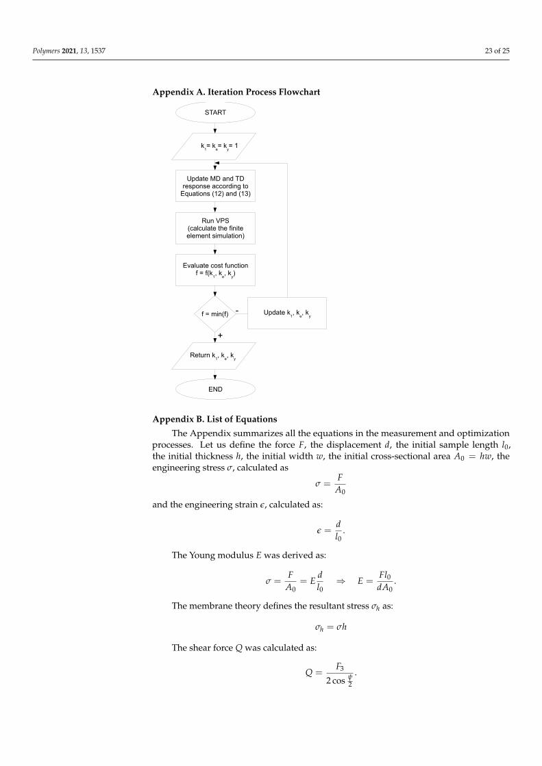
2. Run the VPS simulation to get as(ti) for i ∈ {1, 2, . . . , m};3. Evaluate the cost function f in Equation (16);4. Repeat the loop from 1 until the cost function f reaches its minimum;5. Return both the MD and TD curves according to Equations (12) and (13) for the
optimized coefficients, k1, ke, and ky.
The optimization loop is illustrated in Appendix A as a flowchart.
εεy2
εy1
σy2
σy1
2. Multiplied by 1/ke
3. M
ultip
lied
by k
y
σ1. Multiplied by 1/(k
1k
e)
Figure 11. Optimization coefficients in Region I.
For each testing scenario with n layers, the material was modeled by single-layeredmembrane elements, where the number of upper and lower layers of the model was speci-fied using the membrane material thickness defined by multiplying the single-layer thick-ness h by the number of layers n, meaning that the resultant stress curves in Equations (3)and (8) were also multiplied by n for the particular model. Both sides of the layers werefixed by boundary conditions representing the attachment to the frame. The sphericalimpactor was modeled as a rigid body situated just above the upper layer and loaded bythe initial velocity v corresponding to the particular height. The vertical acceleration andthe vertical displacement were stored and compared to the experimental data.
3. Results
All equations stated in the paper are summarized in Appendix B. The following figuresand tables summarize the results from the quasi-static tests, as well as the identification ofLLDPE parameters under dynamic loading.
3.1. Quasi-Static Loading
The quasi-static experiments proved that the typical stress versus strain curve forLLDPE was composed of three regions [21]; see Figure 3. A summary of all results obtainedby static experimental measurements under different quasi-static loading velocities using a
Polymers 2021, 13, 1537 12 of 25
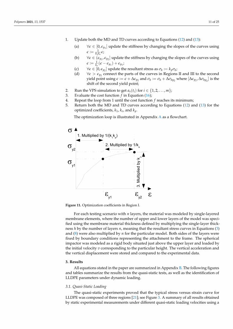
single material layer is displayed in Figure 12. The curves are cut at the positions of thesample ruptures. Table 4 compares the measured experimental properties to those definedby the producer [22].
Table 4. Material properties.
Direction MD TD
Variable Tensile Break Tensile BreakStress (MPa) Elongation (%) Stress (MPa) Elongation (%)
Data sheet [22] 29.2 245 14.1 540Experiment 29.3 139 16.2 701
Error (%) 0.5 −43 15 30
(a) (b)
(c) (d)
Figure 12. Material response in all directions: (a) Force versus displacement in MD. (b) Force versusdisplacement in TD. (c) Force versus displacement in D3. (d) Force versus displacement in D4.
As the quasi-static tests in all three stretching velocities showed similar performance,the curves for each direction were averaged—as shown in Figure 13. It can be seen that thestretching responses in the skewed directions D3 and D4 fit between the MD and TD curves,so no unpredictable behavior during the multi-directional loading should be expected.Therefore, the skewed direction D3 was also used to identify the shear behavior accordingto Equations (4)–(8).
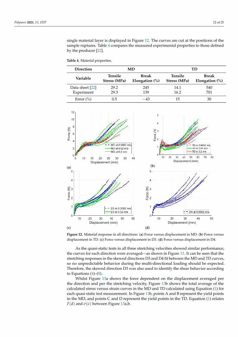
Whilst Figure 13a shows the force dependent on the displacement averaged perthe direction and per the stretching velocity, Figure 13b shows the total average of thecalculated stress versus strain curves in the MD and TD calculated using Equation (1) foreach quasi-static test measurement. In Figure 13b, points A and B represent the yield pointsin the MD, and points C and D represent the yield points in the TD. Equation (1) relatesF(d) and σ(ε) between Figure 13a,b.
Polymers 2021, 13, 1537 13 of 25
(a) (b)
Figure 13. Averaged constitutive material model curves: (a) Force versus displacement averaged perdirection in all stretching velocities. (b) Stress versus strain averaged per direction.
By the detailed analysis of the measured data in Figure 13b, the double yield point [16]from Equations (12) and (13) was observed in both directions. In the MD, the first pointappeared at the stress of σMD
y1 = 8.4 MPa, which corresponded to the strain of εMDy1 =
0.26. The second yield point appeared by reaching the stress of σMDy2 = 20 MPa, which
corresponded to the strain of εMDy2 = 0.84. In TD, the first yield point appeared at the stress
of σTDy1 = 8 MPa, which corresponded to the strain of εTD
y1 = 0.33. The second yield point
appeared before reaching the maximum stress in Region I at the stress of σTDy2 = 10 MPa
corresponding to the strain of εTDy2 = 0.69. Table 5 summarizes the yield points.
Table 5. Yield points (σhy means the resultant yield stress).
Yield PointMD TD
εy (-) σy (MPa) σhy (N/mm) εy (-) σy (MPa) σhy (N/mm)
1 0.26 8.4 0.1 0.33 8 0.12 0.84 20 0.24 0.69 10 0.12
Taking into account the elastic region, the Young modulus E = 50 MPa was identifiedusing Equation (2) by averaging the slopes of the elastic regions of all curves; see Table 6.The average was calculated for the particular directions and stretching velocities firstlyleading to the global average. Both the MD and TD were averaged as they exhibited similarstiffness in the first region.
Table 6. The Young modulus.
Direction MD TD
Stretching0.0002 0.02 0.2 0.0002 0.02 0.2Velocity v (m/s)
Young 44 63 63 67 36 42 54 76 55 41 35 26modulus 57 76 63 47 37 50 39 53 64 47 31 30E (MPa) 63 41 81 70 31 30 55 44 49 58 27 38
Young 57 65 38 53 52 31modulus 53 46
E (MPa) 50
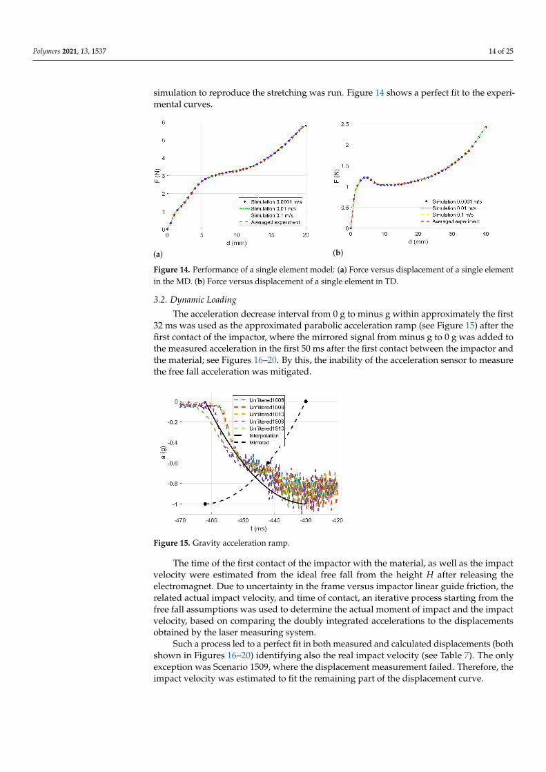
Finally, the resultant constitutive material stress curves developed usingEquations (3) and (8) for a single layer of LLDPE were calculated for the quasi-static load-ing to feed the constitutive material model; see Figure 22. A single-element numerical
Polymers 2021, 13, 1537 14 of 25
simulation to reproduce the stretching was run. Figure 14 shows a perfect fit to the experi-mental curves.
(a) (b)
Figure 14. Performance of a single element model: (a) Force versus displacement of a single elementin the MD. (b) Force versus displacement of a single element in TD.
3.2. Dynamic Loading
The acceleration decrease interval from 0 g to minus g within approximately the first32 ms was used as the approximated parabolic acceleration ramp (see Figure 15) after thefirst contact of the impactor, where the mirrored signal from minus g to 0 g was added tothe measured acceleration in the first 50 ms after the first contact between the impactor andthe material; see Figures 16–20. By this, the inability of the acceleration sensor to measurethe free fall acceleration was mitigated.
Figure 15. Gravity acceleration ramp.
The time of the first contact of the impactor with the material, as well as the impactvelocity were estimated from the ideal free fall from the height H after releasing theelectromagnet. Due to uncertainty in the frame versus impactor linear guide friction, therelated actual impact velocity, and time of contact, an iterative process starting from thefree fall assumptions was used to determine the actual moment of impact and the impactvelocity, based on comparing the doubly integrated accelerations to the displacementsobtained by the laser measuring system.
Such a process led to a perfect fit in both measured and calculated displacements (bothshown in Figures 16–20) identifying also the real impact velocity (see Table 7). The onlyexception was Scenario 1509, where the displacement measurement failed. Therefore, theimpact velocity was estimated to fit the remaining part of the displacement curve.

Polymers 2021, 13, 1537 15 of 25
(a) (b)
Figure 16. Optimization iterations for the drop height H = 10 dm and n = 8 layers: (a) Impactordisplacement. (b) Impactor acceleration.
(a) (b)
Figure 17. Optimization iterations for the drop height H = 10 dm and n = 9 layers: (a) Impactordisplacement. (b) Impactor acceleration.
(a) (b)
Figure 18. Optimization iterations for the drop height H = 10 dm and n = 10 layers: (a) Impactordisplacement. (b) Impactor acceleration.
Polymers 2021, 13, 1537 16 of 25
(a) (b)
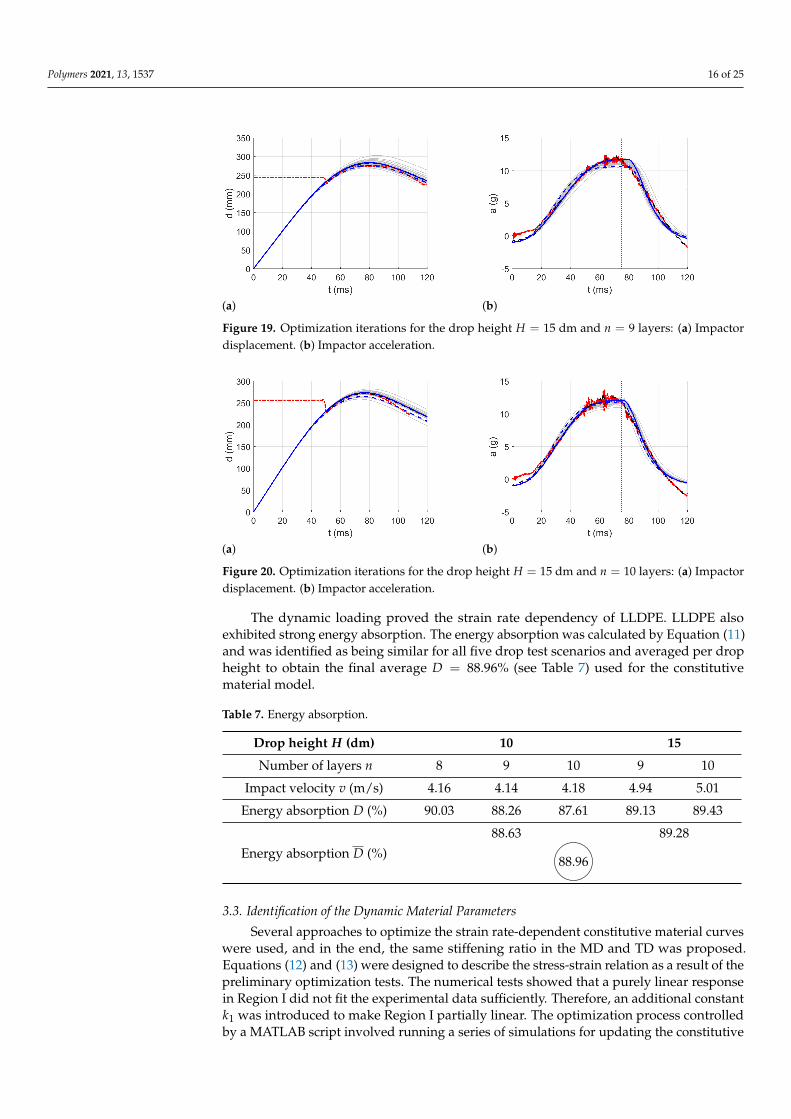
Figure 19. Optimization iterations for the drop height H = 15 dm and n = 9 layers: (a) Impactordisplacement. (b) Impactor acceleration.
(a) (b)
Figure 20. Optimization iterations for the drop height H = 15 dm and n = 10 layers: (a) Impactordisplacement. (b) Impactor acceleration.
The dynamic loading proved the strain rate dependency of LLDPE. LLDPE alsoexhibited strong energy absorption. The energy absorption was calculated by Equation (11)and was identified as being similar for all five drop test scenarios and averaged per dropheight to obtain the final average D = 88.96% (see Table 7) used for the constitutivematerial model.
Table 7. Energy absorption.
Drop height H (dm) 10 15
Number of layers n 8 9 10 9 10
Impact velocity v (m/s) 4.16 4.14 4.18 4.94 5.01
Energy absorption D (%) 90.03 88.26 87.61 89.13 89.43
Energy absorption D (%)88.63 89.28
88.96
3.3. Identification of the Dynamic Material Parameters
Several approaches to optimize the strain rate-dependent constitutive material curveswere used, and in the end, the same stiffening ratio in the MD and TD was proposed.Equations (12) and (13) were designed to describe the stress-strain relation as a result of thepreliminary optimization tests. The numerical tests showed that a purely linear responsein Region I did not fit the experimental data sufficiently. Therefore, an additional constantk1 was introduced to make Region I partially linear. The optimization process controlledby a MATLAB script involved running a series of simulations for updating the constitutive
Polymers 2021, 13, 1537 17 of 25
material model curves. The quasi-static response was taken as the initial guess for theoptimization.
Table 8 shows the coefficients coming from the optimization process. Table 8 alsoshows the number of iterations leading to the optimized constitutive material curves, aswell as the errors from the cost function calculated by Equation (14) and the error in thedisplacement calculated by Equation (15).
Table 8. Optimized coefficients.
Drop height H (dm) 10 15
Number of layers n 8 9 10 9 10
Number of iterations 278 152 205 234 221
First part stiffness multiplier k1 (-) 2.75 2.89 2.99 3.14 3.07Stiffness multiplier ke (-) 3.41 3.47 3.55 1.69 2.29
Yield stress multiplier ky (-) 1.00 0.91 0.88 1.16 1.04
Acceleration error Es (%) 3 3 2 2 3Displacement error Ed (%) 1 1 1 0 1
The intervals for calculating acceleration error are delimited in Figures 16–20 by reddotted vertical lines to consider only the loading, where the iterative processes for theparticular drop heights and the particular number of layers are shown.
The original experimental curves are in red dashed lines. The updated target curves(displacement obtained by integration and acceleration updated by gravity) are shownin dashed black lines. The initial curves (using the static constitutive material model) foroptimization iterations are shown in dashed blue lines. The optimized curves are shown insolid blue lines. The iterative process is shown in solid grey curves.
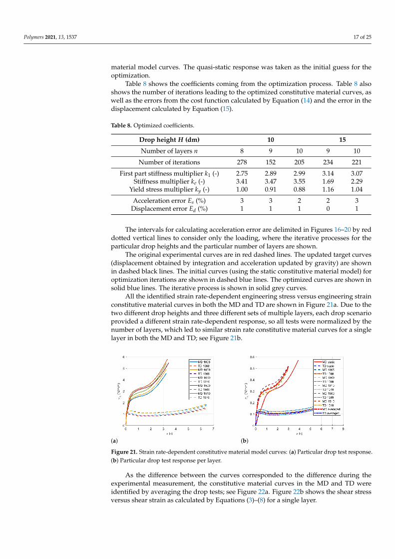
All the identified strain rate-dependent engineering stress versus engineering strainconstitutive material curves in both the MD and TD are shown in Figure 21a. Due to thetwo different drop heights and three different sets of multiple layers, each drop scenarioprovided a different strain rate-dependent response, so all tests were normalized by thenumber of layers, which led to similar strain rate constitutive material curves for a singlelayer in both the MD and TD; see Figure 21b.
(a) (b)
Figure 21. Strain rate-dependent constitutive material model curves: (a) Particular drop test response.(b) Particular drop test response per layer.
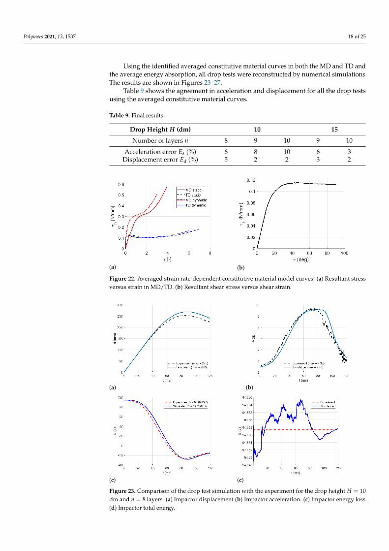
As the difference between the curves corresponded to the difference during theexperimental measurement, the constitutive material curves in the MD and TD wereidentified by averaging the drop tests; see Figure 22a. Figure 22b shows the shear stressversus shear strain as calculated by Equations (3)–(8) for a single layer.
Polymers 2021, 13, 1537 18 of 25
Using the identified averaged constitutive material curves in both the MD and TD andthe average energy absorption, all drop tests were reconstructed by numerical simulations.The results are shown in Figures 23–27.
Table 9 shows the agreement in acceleration and displacement for all the drop testsusing the averaged constitutive material curves.
Table 9. Final results.
Drop Height H (dm) 10 15
Number of layers n 8 9 10 9 10
Acceleration error Es (%) 6 8 10 6 3Displacement error Ed (%) 5 2 2 3 2
(a) (b)
Figure 22. Averaged strain rate-dependent constitutive material model curves: (a) Resultant stressversus strain in MD/TD. (b) Resultant shear stress versus shear strain.
(a) (b)
(c) (c)
Figure 23. Comparison of the drop test simulation with the experiment for the drop height H = 10dm and n = 8 layers: (a) Impactor displacement (b) Impactor acceleration. (c) Impactor energy loss.(d) Impactor total energy.
Polymers 2021, 13, 1537 19 of 25
(a) (b)
(c) (c)
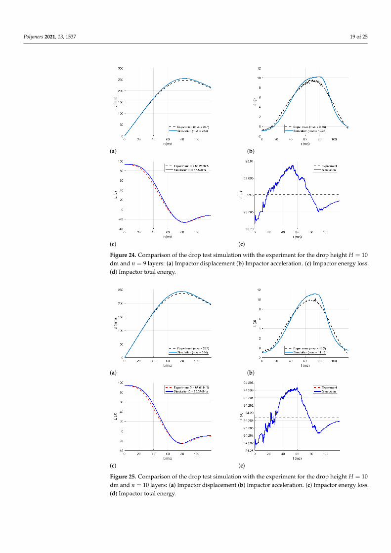
Figure 24. Comparison of the drop test simulation with the experiment for the drop height H = 10dm and n = 9 layers: (a) Impactor displacement (b) Impactor acceleration. (c) Impactor energy loss.(d) Impactor total energy.
(a) (b)
(c) (c)
Figure 25. Comparison of the drop test simulation with the experiment for the drop height H = 10dm and n = 10 layers: (a) Impactor displacement (b) Impactor acceleration. (c) Impactor energy loss.(d) Impactor total energy.
Polymers 2021, 13, 1537 20 of 25
(a) (b)
(c) (c)
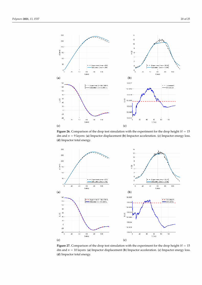
Figure 26. Comparison of the drop test simulation with the experiment for the drop height H = 15dm and n = 9 layers: (a) Impactor displacement (b) Impactor acceleration. (c) Impactor energy loss.(d) Impactor total energy.
(a) (b)
(c) (c)
Figure 27. Comparison of the drop test simulation with the experiment for the drop height H = 15dm and n = 10 layers: (a) Impactor displacement (b) Impactor acceleration. (c) Impactor energy loss.(d) Impactor total energy.
Polymers 2021, 13, 1537 21 of 25
Figure 23 compares the simulation to the experimental drop test for the drop heightH = 10 dm and the number of layers n = 8. Figure 24 compares the simulation tothe experimental drop test for the drop height H = 10 dm and the number of layersn = 9. Figure 25 compares the simulation to the experimental drop test for the drop heightH = 10 dm and the number of layers n = 10. Figure 26 compares the simulation to theexperimental drop test for the drop height H = 15 dm and the number of layers n = 9.Figure 27 compares the simulation to the experimental drop test for the drop height H = 15dm and the number of layers n = 10.
4. Discussion
The quasi-static experiments were performed in two perpendicular directions sup-ported by measurements in two skewed directions. Although the MD and TD exhibiteddifferent loading behavior, the measurements in the skewed directions supported the factthat there was no unexpected behavior during loading in any auxiliary direction.
Table 4 shows a good agreement with the factory data of the quasi-static experimentaltest regarding the tensile stress in both directions. The break elongation was 30% higherin the TD and 43% lower in the MD when compared to the material data sheet in Table 1,which might be caused by the laboratory conditions and influenced by the specimen size.The experimental measurements also confirmed previous studies showing that LLDPE isstiffer in the MD compared to the TD [3,5,6,15].
Table 5 summarizes the yield stresses σMDy = 8.4 MPa and σTD
y = 8 MPa, as well as theyield strains εMD
y = 0.26 and εTDy = 0.33, which were comparable to the values presented
in the literature [21], where the yield stress σy = 9.9 MPa and the yield strain ε = 0.33.However, the elongation at break was measured equal to 1045%, which was higher thanthose measured and stated by the material data sheet. The Young modulus in Table 6 E =50 MPa also showed a comparable value to the published values [21], where the Youngmodulus was experimentally identified as E = 64 MPa.
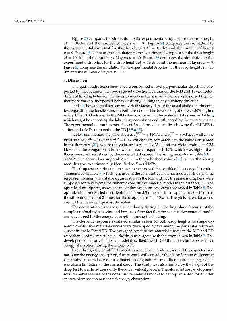
The drop test experimental measurements proved the considerable energy absorptionsummarized in Table 7, which was used in the constitutive material model for the dynamicresponse. To maintain a stable optimization in the MD and TD, the same multipliers weresupposed for developing the dynamic constitutive material model in the MD and TD. Theoptimized multipliers, as well as the optimization process errors are stated in Table 8. Theoptimization process led to stiffening of about 3.5 times for the drop height H =10 dm asthe stiffening is about 2 times for the drop height H =15 dm. The yield stress balancedaround the measured quasi-static value.
The acceleration error was calculated only during the loading phase, because of thecomplex unloading behavior and because of the fact that the constitutive material modelwas developed for the energy absorption during the loading.
The dynamic response exhibited similar values for both drop heights, so single dy-namic constitutive material curves were developed by averaging the particular responsecurves in the MD and TD. The averaged constitutive material curves in the MD and TDwere then used to recalculate all the drop tests again with the error shown in Table 9. Thedeveloped constitutive material model described the LLDPE film behavior to be used forenergy absorption during the impact well.
Even though the identified constitutive material model described the expected sce-nario for the energy absorption, future work will consider the identification of dynamicconstitutive material curves for different loading patterns and different drop energy, whichwas also a limitation of the current study. The study was also limited by the height of thedrop test tower to address only the lower velocity levels. Therefore, future developmentwould enable the use of the constitutive material model to be implemented for a widerspectra of impact scenarios with energy absorption.
Polymers 2021, 13, 1537 22 of 25
5. Conclusions
The paper contributed to the field of virtual testing by developing a material modeland identifying its constitutive parameters. The target material was LLDPE, a materialtraditionally used for packaging goods to protect them during transportation. The paperproved the high energy absorption of the material suitable for impact protection, alsodue to its low weight. Both the quasi-static and dynamic responses of the material wereconsidered in the constitutive material model.
Besides the identification of the constitutive material parameter for both the quasi-static and dynamic responses, the paper provided a complex description of the experimen-tal measurements. While the quasi-static response was measured using a unilateral stretchmeasurement in the MD and TD, the dynamic tests employed a sphere impact using adrop tower.
The quasi-static response was analyzed and evaluated based on the measurement ofseveral samples providing the final curves describing the resultant stress dependent on thestrain in the MD and TD. Those quasi-static curves served as initial values for the dynamicresponse, which was optimized by aligning the experimental and calculated accelerationsof the impactor.
A good agreement of the experimental and model results was achieved and reported,providing the linear low-density polyethylene material model for virtual testing.
Author Contributions: Conceptualization, L.H.; data curation, L.H.; formal analysis, L.H., J.Š., andR.C.; funding acquisition, L.H.; investigation, P.K., T.B., J.Š., S.K., R.K., and L.H.; methodology, L.H. andJ.Š.; project administration, L.H.; resources, P.K.; software, J.Š., L.H., R.C., and M.P.; supervision, L.H.;validation, L.H. and J.Š.; visualization, L.H.; writing—original draft preparation, L.H.; writing—reviewand editing, L.H., P.K., J.Š., T.B., R.K., S.K., R.C., and M.P. All authors read and agreed with the publishedversion of the manuscript.
Funding: This research was funded by the John H. and Amy Bowles Lawrence Foundation, by theEuropean Regional Development Fund-Project Grant Number CZ.02.1.01/0.0/0.0/17_048/0007280and by the University of West Bohemia Grant Number SGS-2019-002.
Data Availability Statement: The data presented in this study are openly available in zenodo athttps://doi.org/10.5281/zenodo.4745000.
Acknowledgments: The authors thank Alojz Hanuliak for donating the testing material roll used forthe experiments.
Conflicts of Interest: The authors declare no conflict of interest. The funders had no role in the designof the study; in the collection, analyses, or interpretation of data; in the writing of the manuscript;nor in the decision to publish the results.
AbbreviationsThe following abbreviations are used in this manuscript:
LLDPE Linear low-density polyethyleneMD Machine directionTD Transverse directionD3 Skewed direction by 45◦
D4 Skewed direction by −45◦
VPS Virtual Performance Solution
Polymers 2021, 13, 1537 23 of 25
Appendix A. Iteration Process Flowchart
START
k1= k
e= k
y= 1
Update MD and TDresponse according to
Equations (12) and (13)
Run VPS(calculate the finiteelement simulation)
Evaluate cost functionf = f(k
1, k
e, k
y)
f = min(f)
END
Return k1, k
e, k
y
+
- Update k1, k
e, k
y
Appendix B. List of Equations
The Appendix summarizes all the equations in the measurement and optimizationprocesses. Let us define the force F, the displacement d, the initial sample length l0,the initial thickness h, the initial width w, the initial cross-sectional area A0 = hw, theengineering stress σ, calculated as
σ =F
A0
and the engineering strain ε, calculated as:
ε =dl0
.
The Young modulus E was derived as:
σ =F
A0= E
dl0
⇒ E =Fl0dA0
.
The membrane theory defines the resultant stress σh as:
σh = σh
The shear force Q was calculated as:
Q =F3
2 cos ψ2
.
Polymers 2021, 13, 1537 24 of 25
The shear angle γ was calculated as:
γ =π
2− ψ
and the deformed sample angle was calculated as:
cosψ
2=
√2L + d2L
.
The shear stress τ was then calculated as:
τ =QLh
and the resultant shear stress was calculated as:
τh = τh =QL
.
Defining the average head mass m, the impactor mass M, the impactor initial velocityv0, the drop height H, and the gravity acceleration g, the energy balance equation wascalculated as:
12
mv20 = MgH.
Defining the impactor displacement d(t) and the impactor acceleration a(t) at anytime, the total energy E(t) was calculated at any time step as:
E(t) = Ek + Ep + W =12
Mv(t)2 + Mgd(t) +
d(t)∫0
Ma(t)ds.
If Eu and El are the energy difference during the loading and unloading phase, respec-tively, the energy loss D was then calculated as:
D = 1− ∆Eu
∆El.
The resultant stress in the MD and TD was calculated as:
σMDh = kyσMD
h (εMD
I.k1ke
), k1 =
{k ∀εMD
I. ∈ [0, εMDy1 ]
1 ∀εMDI. ∈ (εMD
y1 , εMDy2 ]
σTDh = kyσTD
h (εTD
I.k1ke
), k1 =
{k ∀εTD
I. ∈ [0, εTDy1 ]
1 ∀εTDI. ∈ (εTD
y1 , εTDy2 ]
During the optimization process, the acceleration error Ea was calculated as:
Ea =‖as(t)− ae(t)‖‖ae(t)‖
∣∣∣t∈[t1,t2]
and the displacement error Ea was calculated as:
Ed =‖ds(t)− de(t)‖‖de(t)‖
∣∣∣t∈[t1,t2]
.

Polymers 2021, 13, 1537 25 of 25
References1. Špicka, J.; Hyncík, L.; Kovár, L.; Hanuliak, A. Virtual assessment of advanced safety systems for new mobility modes. In
Proceedings of the 16th International Symposium on Computer Methods in Biomechanics and Biomedical Engineering and the4th Conference on Imaging and Visualization, New York, NY, USA, 14–16 August 2019; Columbia University: New York, NY,USA, 2019; p. 263.
2. Hanuliak, A. Safety Restraint System for Motor Vehicles. WO2018/219371, 6 December 2018.3. Mezghani, K.; Furquan, S. Analysis of dart impact resistance of low-density polyethylene and linear low-density polyethylene
blown films via an improved instrumented impact test method. J. Plast. Film. Sheeting 2012, 28, 298–313. [CrossRef]4. Ragaert, K.; Delva, L.; Van Damme, N.; Kuzmanovic, M.; Hubo, S.; Cardon, L. Microstructural foundations of the strength and
resilience of LLDPE artificial turf yarn. Appl. Polym. Sci. 2016, 133, 1–12. [CrossRef]5. Bosi, F.; Pellegrino, S. Molecular based temperature and strain rate dependent yield criterion for anisotropic elastomeric thin
films. Polymer 2017, 125, 144–153. [CrossRef]6. Bosi, F.; Pellegrino, S. Nonlinear thermomechanical response and constitutive modeling of viscoelastic polyethylene membranes.
Mech. Mater. 2018, 117, 9–21. [CrossRef]7. Jeon, K.; Krishnamoorti, R. Morphological behavior of thin linear low-density polyethylene films. Macromolecules 2008,
49, 7131–7140. [CrossRef]8. Morris, B.A. Strength, stifffness, and abuse resistance. In The Science and Technology of Flexible Packaging; Elsevier: Oxford, UK,
2017; pp. 309–350.9. Omar, M.F.; Akil, H.M.; Ahmad, Z.A. Effect of molecular structures on dynamic compression properties of polyethylene. Mater.
Sci. Eng. A 2012, 538, 125–134. [CrossRef]10. Jordan, J.; Casem, D.T.; Bradley, J.M.; Dwivedi, A.K. Mechanical Properties of Low Density Polyethylene. J. Dyn. Behav. Mater.
2016, 2, 411–420. [CrossRef]11. Zhang, X.M.; Elkoun, S.; Ajji, A.; Huneault, M.A. Oriented structure and anisotropy properties of polymer blown films: HDPE,
LLDPE and LDPE. Polymer 2004, 45, 217–229. [CrossRef]12. Ren, Y.; Shi, Y.; Yao, X.; Tang, Y.; Liu, L.-Z. Different Dependence of Tear Strength on Film Orientation of LLDPE Made with
Different Co-Monomer. Polymers 2019, 11, 434. [CrossRef]13. Dogru, S.; Aksoy, B.; Bayraktar, H.; Alaca, B.E. Poisson’s ratio of PDMS thin films. Polym. Test. 2018, 69, 375–384. [CrossRef]14. Dorigato, A.; Pegoretti, A.; Kolarík, J. Nonlinear tensile creep of linear low density polyethylene/fumed silica nanocomposites:
Time-strain superposition and creep prediction. Polym. Compos. 2010, 31, 1947–1955. [CrossRef]15. Krishnaswamy, K.R.; Lamborn, M.J. Tensile Properties of Linear Low Density Polyethylene (LLDPE) Blown Films. Polym. Eng.
Sci. 2000, 40, 2395–2396. [CrossRef]16. Plaza, A.R.; Ramos, E.; Manzur, A.; Olayo, R.; Escobar, A. Double yield points in triblends of LDPE, LLDPE and EPDM. J. Mater.
Sci. 1997, 32, 549–554. [CrossRef]17. Richeton, J.; Ahzi, S.; Daridon, L.; Rémond, Y. Modeling of strain rates and temperature effects on the yield behavior of amorphous
polymers. J. Phys. IV (Proc.) 2003, 110, 39–44. [CrossRef]18. Luyt, A.S.; Gasmi, S.A.; Malik, S.S.; Aljindi, R.M.; Ouederni, M.; Vouyiouka, S.N.; Porfyris, A.D.; Pfaendner, R.; Papaspyrides,
C.D. Artificial weathering and accelerated heat aging studies on low-density polyethylene (LDPE) produced via autoclave andtubular process technologies. eXPRESS Polym. Lett. 2021, 15, 121–136. [CrossRef]
19. Du, W.; Ren, Y.; Tang, Y.; Shi, Y.; Yao, X.; Zheng, C.; Zhang, X.; Guo, M.; Zhang, S.; Liu, L.Z. Different structure transitions andtensile property of LLDPE film deformed at slow and very fast speeds. Eur. Polym. J. 2018, 103, 170–178. [CrossRef]
20. Omar, M.F. Static and Dynamic Mechanical Properties of Thermoplastic Materials; Lap Lambert Academic Publishing: Chisinau,Moldova, 2013.
21. Durmus, A.; Kasgöz, A.; Macoscom, C.W. Mechanical Properties of Linear Low-density Polyethylene (LLDPE)/clay Nanocom-posites: Estimation of Aspect Ratio and Interfacial Strength by Composite Models. Macromol. Sci. Part B Phys. 2008, 47, 608–619.[CrossRef]
22. LLDPE Foils. 2020. Available online: http://www.tichelmann.cz/lldpe-folie (accessed on 21 November 2020).23. ASTM Standards. 2021. Available online: https://www.astm.org (accessed on 17 March 2021).24. ESI Group International. VPS User’s Manual; ESI Group International: Paris, France, 2020.25. Vezin, P.; Bruyère-Garnier, K.; Bermond, F.; Verriest, J.P. Comparison of Hybrid III, Thor-α and PMHS response in frontal sled
tests. Stapp Car Crash J. 2002, 46, 1–26. [PubMed]26. Yoganandan, N.; Pintar, F.A.; Zhang, J.; Baisden, J.L. Physical properties of the human head: Mass, center of gravity and moment
of inertia. J. Biomech. 2009, 42, 1177–1192. [CrossRef] [PubMed]27. Cichos, D.; de Vogel, D.; Otto, M.; Schaar, O.; Zoelsch, S.; Clausnitzer, S.; Vetter, D. Crash Analysis Criteria Description. 2011.
Available online: http://mdvfs.org/crash-analyse (accessed on 9 May 2021).28. Gupalov, V.; Kukaev, A.; Shevchenko, S.; Shalymov, E.; Venediktov, V. Physical principles of a piezo accelerometer sensitive to a
nearly constant signal. Sensors 2018, 18, 3258. [CrossRef] [PubMed]