IOP PUBLISHING MEASUREMENT SCIENCE AND TECHNOLOGY

Meas. Sci. Technol. 22 (2011) 055701 (12pp) doi:10.1088/0957-0233/22/5/055701

Identification of multiple characteristiccomponents with high accuracy andresolution using the zoom interpolateddiscrete Fourier transformQiang Miao1,4, Lin Cong1 and Michael Pecht2,3

1 School of Mechanical, Electronic and Industrial Engineering, University of Electronic Science andTechnology of China, Chengdu, Sichuan 611731, People’s Republic of China2 Center for Advanced Life Cycle Engineering (CALCE), University of Maryland, College Park,MD 20742, USA3 Center for Prognostics and System Health Management, City University of Hong Kong, Hong Kong

E-mail: mqiang@uestc.edu.cn

Received 5 July 2010, in final form 10 January 2011Published 23 March 2011Online at stacks.iop.org/MST/22/055701

AbstractComplex systems can significantly benefit from condition monitoring and diagnosis tooptimize operational availability and safety. However, for most complex systems, multi-faultdiagnosis is a challenging issue, as fault-related components are often too close in thefrequency domain to be easily identified. In this paper, the interpolated discrete Fouriertransform (IpDFT) with maximum sidelobe decay windows is investigated for machinery faultfeature identification. A novel identification method called the zoom IpDFT is proposed,which combines the idea of local frequency band zooming-in with the IpDFT anddemonstrates high accuracy and frequency resolution in signal parameter estimation whendifferent characteristic frequencies are very close. Simulation and a case study on rollingelement bearing vibration data indicate that the proposed zoom IpDFT based on multiplemodulations has better capability to identify characteristic components than do traditionalmethods, including fast Fourier transform (FFT) and zoom FFT.

Keywords: prognostics and health management, interpolated DFT, zoom IpDFT, Fouriertransform, characteristic component identification

(Some figures in this article are in colour only in the electronic version)

1. Introduction

The rapid development of complex systems such as powerplants, high-speed transportation vehicles and high-precisionmachining centers has been emphasizing the need for conditionmonitoring and diagnosis so as to maximize operationalavailability and safety [1]. Therefore, research on prognosticsand health management (PHM) has attracted the interest ofindustry and academia due to its great potential to addressthese needs [2]. In the process of PHM implementation,data preprocessing and feature extraction are the fundamental

4 Author to whom any correspondence should be addressed.

modules, since their outputs are used for system healthassessment and prediction [2, 3]. However, the complicatedstructures and working conditions of complex systems mayresult in multiple faults during their operation that producemulti-frequency signals and lead to a challenging problemcalled multi-fault diagnosis. In these situations, frequencyaliasing arises, and fault-related components may be too closein the frequency domain to be effectively identified for furtherfeature extraction and diagnosis.

The identification of characteristic components isfundamental and important for complex system featureextraction and health assessment [4]. Along with the

0957-0233/11/055701+12$33.00 1 © 2011 IOP Publishing Ltd Printed in the UK & the USA

Meas. Sci. Technol. 22 (2011) 055701 Q Miao et al

development of signal processing, more and more techniqueshave been introduced to diagnose faults in machinery[5]. The methods used for characteristic componentidentification or fault character extraction usually can beclassified into frequency domain and time domain methods.Time domain methods provide high frequency selectivityand high estimation accuracy, but require computation-intensive algorithms to determine the optimal model order[6]. Frequency domain methods use the discrete Fouriertransform (DFT) to calculate the spectrum and estimate thefrequency parameters of a signal. On account of someinherent drawbacks, the traditional DFT-based approacheshave some restrictions in practice. For example, it is hard toobtain accurate frequency, amplitude and phase informationabout synchronous vibration and its harmonic or subharmoniccomponents because of the leakage and the picket-fence effectof the DFT spectrum [7].

In order to enhance the efficiency and accuracy of faultdiagnosis, it is crucial to improve the estimation accuracy ofamplitude, frequency and phase of signal for feature extractionin the frequency domain. The method used to deal withthis problem is called ‘windowing’. One frequency domainmethod often used for estimating multi-frequency signalparameters under noncoherent sampling is the interpolatedDFT (IpDFT) method, which provides very accurate parameterestimates. For example, Ramos and Serra [8] compared thefrequency algorithms of IpDFT, Chirp-Z transform, Hilberttransform, STFT, CWT, MUSIC, Sine-fit and Kalman filtering.They determined that the IpDFT algorithm is the mostprecise, accurate and fastest algorithm. Rife and Vincent[9] proposed a specific approach, called the interpolatedfast Fourier transform (IFFT), to dramatically improve theaccuracy of the FFT spectrum. Moreover, Jain et al [10]proposed an approximate interpolation algorithm to obtainaccurate amplitude, phase and frequency information whena rectangular window is employed. Shi et al [11] proposed thegeneral IFFT for diagnosing faults in large rotating machinery,but the algorithm is very complicated.

The performance of the IpDFT method depends on thewindow used [12], and it should be noted that the formulas forestimating the parameters of a multi-frequency signal are verycomplicated for most windows. Among all these windows, themaximum sidelobe decay windows are frequently employedin the IpDFT method. The IpDFT method with maximumsidelobe decay windows leads to very accurate estimates, sincethe parameters of a multi-frequency signal can be estimated byanalytical formulas [13, 14]. Belega and Dallet [15] proposedaccurate and simple formulas for estimating the variances ofthe estimators of the parameters of a multi-frequency signalobtained by the IpDFT method with maximum sidelobe decaywindows.

The goal of this paper is to investigate the potentialof the IpDFT with maximum sidelobe decay windows inmachinery (e.g., gearbox, bearing) feature extraction andcondition monitoring. An IpDFT-based method combiningthe idea of local frequency band zooming-in (i.e. the zoomIpDFT) is proposed in this research to further improve theidentification capability of multiple adjacent characteristic

components in the frequency domain, which is a challengingissue for complex system condition monitoring and PHM.

The organization of this paper is as follows. Section 2gives a brief description of the IpDFT. A novel method ofzoom IpDFT based on multiple modulations is proposed insection 3 to solve the problem of high frequency resolution infault characteristic frequency identification. Section 4 furtherinvestigates and validates the proposed method with rollingelement bearing vibration data. Conclusions are summarizedin section 5.

2. The interpolated DFT

2.1. The interpolated DFT with maximum sidelobe decaywindows

The maximum sidelobe decay windows are the cosinewindows. An H-term (H > 1) maximum sidelobe decaywindow has the most rapidly decaying sidelobes, equal to6(2H − 1) dB/octave. It can be defined as

w(m) =H−1∑h=0

(−1)hah cos(

2πhm

M

), m = 0, 1, . . . ,M − 1

(1)

where ah are the coefficients of the H-term maximum sidelobedecay window [15] and M is the number of samples. ah canbe expressed as

a0 = CH−12H−2

22H−2, ah = CH−h−1

2H−2

22H−3, h = 1, 2, . . . , H − 1 (2)

where Cpm = m!

(m−p)!p! .

The discrete-time Fourier transform (DTFT) of w(m) isgiven by

W(λ) = sin(πλ)e−jπλej πM

λ

H−1∑h=0

(−1)h0.5ah

×[

e−j πM

λ

sin πM

(λ − h)+

ej πM

λ

sin πM

(λ + h)

], λ ∈ [0,M). (3)

For M � 1, the DTFT of the H-term maximum sidelobe decaywindow can be written as [8]

W(λ) = M sin(πλ)

22H−2πλe−jπλej π

Mλ (2H − 2)!∏H−1

h=1 (h2 − λ2). (4)

Now, let us consider a multi-frequency signal x(t) with asampling frequency fs

x(m) = A0 +K∑

k=1

Ak sin

(2π

fk

fs

m + ϕk

),

m = 0, 1, . . . ,M − 1 (5)

where K is the number of frequency components; Ak , fk andϕk are, respectively, the amplitude, frequency and phase ofthe kth component; A0 is the offset; and M is the numberof samples. In order to reduce the leakage error, x(m) is

2

Meas. Sci. Technol. 22 (2011) 055701 Q Miao et al

multiplied by a suitable window sequence w(m). Thus, theDFT of the resulting signal xw = x(m)w(m) is given by

XW(λ) = A0W(λ)

+K∑

k=1

Ak

2j[W(λ − λk)e

jϕk − W(λ + λk)e−jϕk ], λ ∈ [0,M)

(6)

where λ represents the normalized frequency expressed in bins,W(λ) is the DTFT of w(m) and λk = fk

f0, f0 = fs

M.

If W(λ) exhibits sidelobes at a negligible level and if theminimum distance between spectral lines is larger than themain lobe band width (MLBW) expressed in bins, then forλ ∼= λk , equation (6) becomes

XW(λ) ∼= Ak

2jW(λ − λk)e

jϕk , k = 1, 2, . . . , K. (7)

The relationship between the frequencies fk and fs is given by

fk

fs

= λk

M= lk + δk

M, k = 1, 2, . . . , K (8)

where lk and δk are, respectively, the integer part and thefractional part of λk with δk ∈ [−0.5, 0.5); lk is the index ofthe largest discrete spectrum module corresponding to the kthcomponent. The IpDFT method is used to estimate δk . Forthis purpose, αk is defined as

αk =

⎧⎪⎪⎨⎪⎪⎩

|XW(lk)||XW(lk − 1)| , if − 0.5 � δk < 0

|XW(lk + 1)||XW(lk)| , if 0 � δk < 0.5

. (9)

From the above expression it follows that δk can be estimatedby

δk∼=

⎧⎪⎪⎨⎪⎪⎩

(H − 1)αk − H

αk + 1, if − 0.5 � δk < 0

Hαk − H + 1

αk + 1, if 0 � δk < 0.5

. (10)

From (8) and (10) the frequency of the kth component can beestimated by

f k∼=

⎧⎪⎪⎪⎨⎪⎪⎪⎩

(lk +

(H − 1)αk − H

αk + 1

)f0, if − 0.5 � δk < 0

(lk +

Hαk − H + 1

αk + 1

)f0, if 0 � δk < 0.5.

(11)

Using (4) and (7), the amplitude of the kth component can beestimated by

Ak = 22H−1πδk|XW(lk)|M sin(πδk)(2H − 2)!

H−1∏h=1

(h2 − δ2

k

). (12)

From an accurate estimation of the phase associated with thekth component, equation (7) is used in which the window’sDTFT is computed by (13)

ϕk = phase{XW(lk)} − πδk + πδk

M− π

2sign(δk)

− phase{W0(−δk)} (13)

Table 1. Estimation of the parameters by the IpDFT.

Frequency (Hz) Amplitude Phase

The first f 1 = 20.2869 A1 = 1.5004 ϕ1 = 0.2898componentThe second f 2 = 90.7004 A2 = 2.0000 ϕ2 = 0.4976componentThe third f 3 = 171.7000 A3 = 1.7000 ϕ3 = 0.1002component

where

W0(λ) =H−1∑h=0

(−1)h0.5ah

[e−j π

Mλ

sin πM

(λ − h)+

ej πM

λ

sin πM

(λ + h)

],

λ ∈ [0,M)

sign(·) is the sign function, and

sign(δk) ={−1, if − 0.5 � δk < 0

1, if 0 � δk < 0.5

2.2. Investigation of the IpDFT using a simulation example

In order to explore the accurate parameter estimation of amulti-frequency signal by the IpDFT method with maximumsidelobe decay windows, a simulated time domain signalcontaining three components is analyzed as follows:

x(n) =3∑

k=1

Ak sin

(2πn

fk

fs

+ ϕk

)+ rand(s),

n = 0, 1, . . . , N − 1 (14)

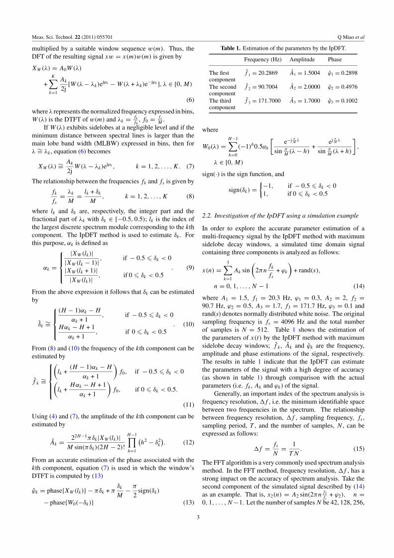
where A1 = 1.5, f1 = 20.3 Hz, ϕ1 = 0.3, A2 = 2, f2 =90.7 Hz, ϕ2 = 0.5, A3 = 1.7, f3 = 171.7 Hz, ϕ3 = 0.1 andrand(s) denotes normally distributed white noise. The originalsampling frequency is fs = 4096 Hz and the total numberof samples is N = 512. Table 1 shows the estimation ofthe parameters of x(t) by the IpDFT method with maximumsidelobe decay windows; f k , Ak and ϕk are the frequency,amplitude and phase estimations of the signal, respectively.The results in table 1 indicate that the IpDFT can estimatethe parameters of the signal with a high degree of accuracy(as shown in table 1) through comparison with the actualparameters (i.e. fk , Ak and ϕk) of the signal.

Generally, an important index of the spectrum analysis isfrequency resolution, �f , i.e. the minimum identifiable spacebetween two frequencies in the spectrum. The relationshipbetween frequency resolution, �f , sampling frequency, fs ,sampling period, T , and the number of samples, N , can beexpressed as follows:

�f = fs

N= 1

T N. (15)

The FFT algorithm is a very commonly used spectrum analysismethod. In the FFT method, frequency resolution, �f , has astrong impact on the accuracy of spectrum analysis. Take thesecond component of the simulated signal described by (14)as an example. That is, x2(n) = A2 sin(2πn

f2

fs+ ϕ2), n =

0, 1, . . . , N −1. Let the number of samples N be 42, 128, 256,

3

Meas. Sci. Technol. 22 (2011) 055701 Q Miao et al

500 1000 1500 2000 2500 3000 3500 4000-2

0

2

4

6

8

10

12

14

Bia

s o

f fr

eque

ncy

est

imat

ion(%

)

Sampling point number

FFT method

IpDFT method

Figure 1. Comparison of bias of the frequency estimation.

512, 1024, 2048 and 4096. Define the bias of the frequencyestimation as

bias =∣∣∣∣∣f2 − f 2

f2

∣∣∣∣∣ × 100%. (16)

Figure 1 shows the bias of the frequency estimation using theFFT method and the IpDFT method under different numbersof samples.

The experimental results indicate that the method ofIpDFT can estimate the parameters of the signal with higheraccuracy (i.e. very small bias) compared with the FFT,especially when the number of samples is limited. Thesame conclusion can be obtained in the estimation of biasof amplitude and phase.

3. The zoom IpDFT

3.1. The problem of frequency resolution

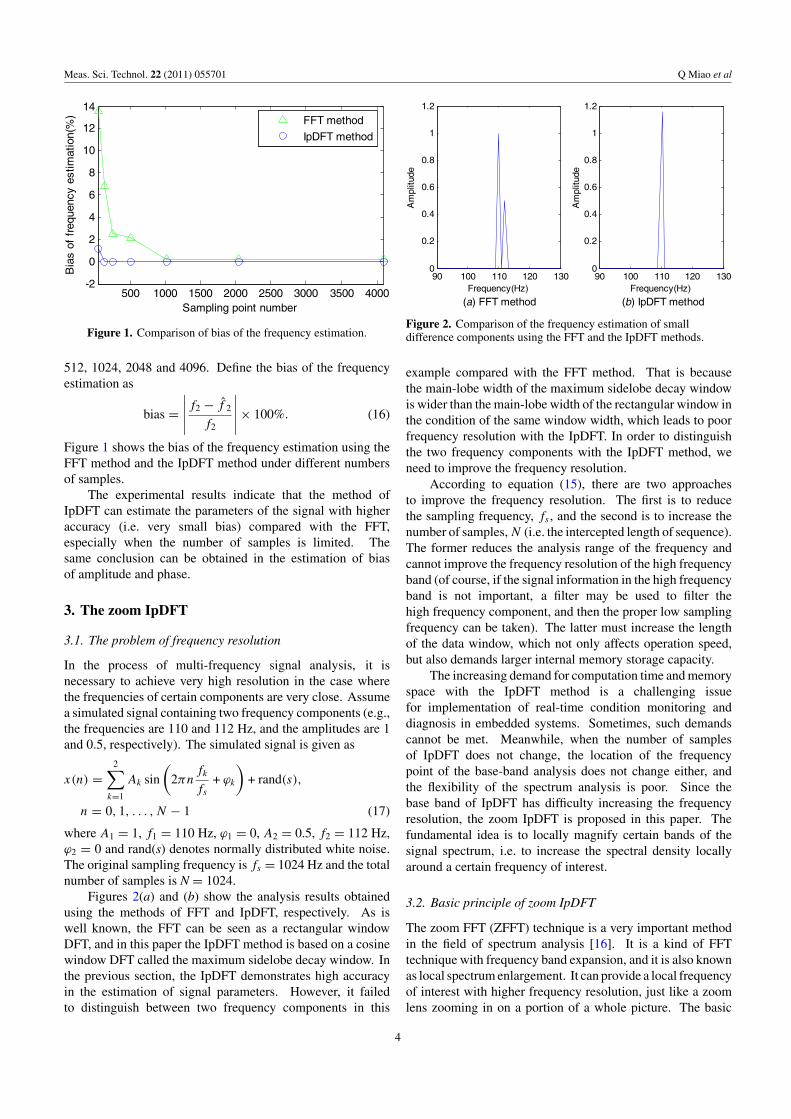
In the process of multi-frequency signal analysis, it isnecessary to achieve very high resolution in the case wherethe frequencies of certain components are very close. Assumea simulated signal containing two frequency components (e.g.,the frequencies are 110 and 112 Hz, and the amplitudes are 1and 0.5, respectively). The simulated signal is given as

x(n) =2∑

k=1

Ak sin

(2πn

fk

fs

+ ϕk

)+ rand(s),

n = 0, 1, . . . , N − 1 (17)

where A1 = 1, f1 = 110 Hz, ϕ1 = 0, A2 = 0.5, f2 = 112 Hz,ϕ2 = 0 and rand(s) denotes normally distributed white noise.The original sampling frequency is fs = 1024 Hz and the totalnumber of samples is N = 1024.

Figures 2(a) and (b) show the analysis results obtainedusing the methods of FFT and IpDFT, respectively. As iswell known, the FFT can be seen as a rectangular windowDFT, and in this paper the IpDFT method is based on a cosinewindow DFT called the maximum sidelobe decay window. Inthe previous section, the IpDFT demonstrates high accuracyin the estimation of signal parameters. However, it failedto distinguish between two frequency components in this

90 100 110 120 1300

0.2

0.4

0.6

0.8

1

1.2

Frequency(Hz)

(a) FFT method

Am

plit

ude

90 100 110 120 1300

0.2

0.4

0.6

0.8

1

1.2

Frequency(Hz)

(b) IpDFT method

Am

plit

ude

Figure 2. Comparison of the frequency estimation of smalldifference components using the FFT and the IpDFT methods.

example compared with the FFT method. That is becausethe main-lobe width of the maximum sidelobe decay windowis wider than the main-lobe width of the rectangular window inthe condition of the same window width, which leads to poorfrequency resolution with the IpDFT. In order to distinguishthe two frequency components with the IpDFT method, weneed to improve the frequency resolution.

According to equation (15), there are two approachesto improve the frequency resolution. The first is to reducethe sampling frequency, fs , and the second is to increase thenumber of samples, N (i.e. the intercepted length of sequence).The former reduces the analysis range of the frequency andcannot improve the frequency resolution of the high frequencyband (of course, if the signal information in the high frequencyband is not important, a filter may be used to filter thehigh frequency component, and then the proper low samplingfrequency can be taken). The latter must increase the lengthof the data window, which not only affects operation speed,but also demands larger internal memory storage capacity.

The increasing demand for computation time and memoryspace with the IpDFT method is a challenging issuefor implementation of real-time condition monitoring anddiagnosis in embedded systems. Sometimes, such demandscannot be met. Meanwhile, when the number of samplesof IpDFT does not change, the location of the frequencypoint of the base-band analysis does not change either, andthe flexibility of the spectrum analysis is poor. Since thebase band of IpDFT has difficulty increasing the frequencyresolution, the zoom IpDFT is proposed in this paper. Thefundamental idea is to locally magnify certain bands of thesignal spectrum, i.e. to increase the spectral density locallyaround a certain frequency of interest.

3.2. Basic principle of zoom IpDFT

The zoom FFT (ZFFT) technique is a very important methodin the field of spectrum analysis [16]. It is a kind of FFTtechnique with frequency band expansion, and it is also knownas local spectrum enlargement. It can provide a local frequencyof interest with higher frequency resolution, just like a zoomlens zooming in on a portion of a whole picture. The basic

4

Meas. Sci. Technol. 22 (2011) 055701 Q Miao et al

Spectrum of sampled signal x(t)

Digital frequency shift

Digital low-pass filtering

Re-sampling

IpDFT transforming

Weighted correction

Figure 3. The implementation of zoom IpDFT based on multiplemodulations.

principle of the zoom IpDFT method is similar to ZFFT, withthe FFT being replaced by the IpDFT. The experimental resultsin figure 1 indicate that the IpDFT is better than the FFT undersatisfactory frequency resolution conditions. Therefore, thezoom IpDFT has the advantages of both higher parameterestimation accuracy (like the IpDFT) and higher frequencyresolution (like ZFFT). This paper mainly discusses the zoomIpDFT method based on multiple modulations.

The implementation of the zoom IpDFT can besummarized by the steps shown in figure 3. The steps includedigital frequency shift, digital low-pass filtering, re-sampling,IpDFT transforming and weighted correction.

Given the original sampling frequency, fs , the frequencycomponents over fs/2 of the continuous signal x(t) are firsteliminated via an anti-superposing low-pass filter, then re-sampled with the frequency fs to get the discrete data x(n)

including N points. Suppose the central frequency of the localband intended to be enlarged is f0 and the frequency bandwidthis B. Then the second step is to carry multiple modulationson the signal x(n), which is realized by multiplying the digitalsignal x(n) by e−j2πnf0/fs . Therefore, the signal after thefrequency shift x0(n) can be expressed as follows:

x0(n) = x(n)e−j2πnf0/fs

= x(n) cos(2πnf0/f ) − jx(n) sin(2πnf0/f ). (18)

According to the frequency shift nature of the discrete Fouriertransform, the discrete spectrum of x0(n) is

X0(k) = X(k + L0) (19)

where L0 = Nf0/fs represents the order number of thespectral line when the frequency is f0; X0(k) is the spectrumafter the frequency shift; and X(k) is the spectrum before thefrequency shift.

179 180 181 182 1830

1

3

5

7

Frequency(Hz)

Am

plit

ude

179 180 181 182 1830

1

3

5

7

Frequency(Hz)

Am

plit

ude

(a) Zoom FFT (b) Zoom IpDFT

Figure 4. Comparison of the frequency and amplitude estimationusing different methods.

Then, all of the frequency components of the signal arefiltered after the frequency shift except for a narrow band Baround f0 via a low-pass filter:

Y0(k) = X0(k)H(k) = X(k + L0)H(k),

k = 0, 1, 2, . . . , N − 1 (20)

where H(k) is the response of the low-pass filter. The outputtime domain signal of the low-pass filter is

y0(n) = 1

N

N−1∑k=0

Y0(k)W−nkN = 1

N

N−1∑k=0

Y0(k)e−j2πnk/N . (21)

Through re-sampling at a new sampling frequency, f ′s =

fs/D, the frequency resolution is enhanced D times whilereducing the sampling frequency and keeping the originallength of record in seconds. That is, the multiple of refining isD, and a new discrete signal xr(n) = y0(Dn) can be obtainedby this process. By applying the complex IpDFT computationto the signal xr(n), the spectral line after refining can bereceived with its central frequency as f0 and bandwidth asB = fs/2D [16].

3.3. Comparison of the zoom FFT and zoom IpDFT using asimulation example

In order to explore the parameter estimation accuracy ofa multi-frequency signal by the zoom IpDFT method withmaximum sidelobe decay windows, a simulated signalcontaining four components is analyzed as follows:

x(t) =4∑

k=1

Ak sin(2πfkt) + rand(s). (22)

Here, A1 = 1, f1 = 180.5 Hz, A2 = 2, f2 = 181 Hz, A3 = 3,f3 = 181.4 Hz, A4 = 7, f4 = 181.9 Hz and rand(s) denotesa normally distributed white noise. The original samplingfrequency is fs = 1024 Hz, the number of samples is N =256 and D = 30. The central frequency of the local band,f0, is 178 Hz. According to the equation B = fs/2D, thebandwidth B is about 17 Hz. Figure 4 shows a comparison of

5

Meas. Sci. Technol. 22 (2011) 055701 Q Miao et al

Figure 5. Test rig for bearings.

frequency and amplitude estimation using the zoom FFT andzoom IpDFT, respectively.

As shown in figure 4, both the zoom FFT method andthe zoom IpDFT method can increase the resolution of thespectrum and obtain good results in frequency estimation.However, for the zoom FFT, the frequency estimation resultis not clear compared with the zoom IpDFT, especially at thefirst signal component frequency of 180.5 Hz. Figure 4 alsodemonstrates that the amplitude estimation with the methodof zoom FFT is not accurate due to the energy leakage ofthe base frequency. Thus, the amplitude error is largercompared with the zoom IpDFT, and it cannot be used forquantitative analysis. Overall, the zoom IpDFT can achievebetter performance in characteristic frequency identification.

4. Case study

In this paper, real motor bearing data picked up with a samplingfrequency of 12k Hz by an accelerometer placed at the driveend of the motor housing were used to validate the proposedmethod. Three kinds of bearing conditions were consideredin this case study, namely the normal condition, the innerrace fault condition and the outer race fault condition. Theaccelerometers under the normal conditions and inner racefault conditions were placed at the 12 o’clock position, whileunder the outer race fault conditions, they were placed at the6 o’clock position. The test rig is shown in figure 5. Singlepoint faults were introduced to normal bearings using electro-discharge machining with a fault diameter of 0.007 inches anda fault depth of 0.011 inches. The specifications of a bearingare shown in table 2. The shaft rotation speed, fr , variedfrom 1730 to 1797 rpm. The characteristic frequencies of thebearing were calculated by the following formulas [17]:

fI = 5.4152 × fr (23)

fO = 3.5848 × fr . (24)

Here, fI and fO are the inner race fault characteristicfrequency and outer race fault characteristic frequency,respectively. There is a total of 12 data sets, including 4 normalbearings, 4 inner race fault bearings, and 4 outer race faultbearings at different rotation speeds and work loads. Table 3shows their corresponding characteristic frequencies.

Table 2. Motor bearing specifications (inches).

Inside diameter 0.9843

Outside diameter 2.0472Thickness 0.5906Ball diameter 0.3126Pitch diameter 1.537

Table 3. Fault characteristic frequencies of bearing at differentrotation speeds and loads.

Motor load Motor speed Inner race Outer race(HP) (rpm) fI (Hz) fO (Hz)

0 1797 162.2 107.41 1772 160.0 105.92 1750 157.9 104.63 1730 156.1 103.4

4.1. Identification of fault characteristic frequencies at amotor speed of 1797 rpm and load HP 0

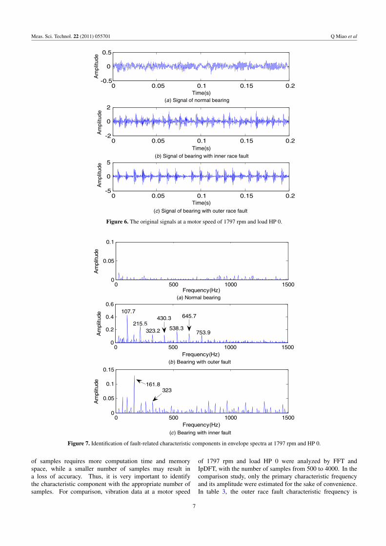
In this section, vibration signals, including normal bearingdata, inner race fault data and outer race fault data at a motorspeed of 1797 rpm and load of HP 0, are used to validatethe proposed method. Figure 6 shows the original vibrationsignals of normal data, inner race fault data and outer race faultdata. In order to enhance the computing efficiency, each pieceof data with 0.2 s is selected for envelope spectrum analysis.Figure 7 shows the identification of fault-related characteristiccomponents at 1797 rpm and HP 0.

Figure 7(a) shows no fault characteristic frequencywhen the bearing was under normal conditions. However,bearings with an inner race fault or an outer race faultcan be identified via their corresponding fault characteristicfrequencies (including harmonics), as shown in figures 7(b)and (c). The estimations of these frequencies are almostconsistent with the corresponding theoretical calculations (seetable 3).

4.2. Identification of fault characteristic frequencies underdifferent working conditions

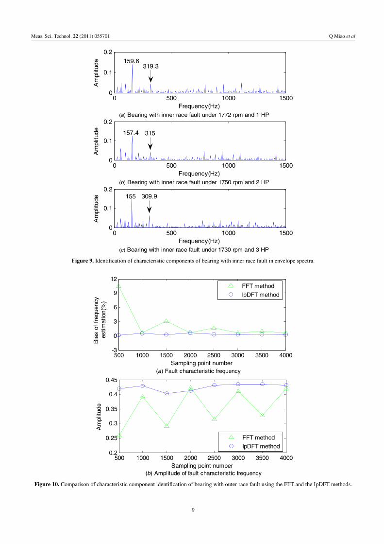
In this section, we consider the influence of different workingconditions, including different rotation speeds and differentloads. Figure 8 shows the analysis results using vibration datafrom a bearing with an outer race fault under different workingconditions. It can be observed that the proposed zoom IpDFTcan identify the outer race fault characteristic frequency, fO ,and its harmonics. In addition, figure 9 gives the analysisresults using a bearing with an inner race fault under differentworking conditions, which also shows good potential for theidentification of a characteristic component, fI .

4.3. Comparison with the traditional FFT in faultcharacteristic identification using the IpDFT

Usually, the number of samples should be chosen accordingto expert experience, working condition or calculation speedwhen utilizing the FFT or the IpDFT. A larger number

6

Meas. Sci. Technol. 22 (2011) 055701 Q Miao et al

0 0.05 0.1 0.15 0.2-0.5

0

0.5

0 0.05 0.1 0.15 0.2-2

0

2

0 0.05 0.1 0.15 0.2-5

0

5

Am

plit

ud

e

Am

plit

ud

eA

mp

litu

de

Time(s)

Time(s)

Time(s)

(a) Signal of normal bearing

(b) Signal of bearing with inner race fault

(c) Signal of bearing with outer race fault

Figure 6. The original signals at a motor speed of 1797 rpm and load HP 0.

0 500 1000 15000

0.05

0.1

Frequency(Hz)

Am

plit

ude

(a) Normal bearing

0 500 1000 15000

0.2

0.4

0.6

Frequency(Hz)

Am

plitu

de

(b) Bearing with outer fault

0 500 1000 15000

0.05

0.1

0.15

Frequency(Hz)

Am

plitu

de

(c) Bearing with inner fault

107.7

215.5323.2

430.3

538.3

645.7

753.9

323161.8

Figure 7. Identification of fault-related characteristic components in envelope spectra at 1797 rpm and HP 0.

of samples requires more computation time and memoryspace, while a smaller number of samples may result ina loss of accuracy. Thus, it is very important to identifythe characteristic component with the appropriate number ofsamples. For comparison, vibration data at a motor speed

of 1797 rpm and load HP 0 were analyzed by FFT andIpDFT, with the number of samples from 500 to 4000. In thecomparison study, only the primary characteristic frequencyand its amplitude were estimated for the sake of convenience.In table 3, the outer race fault characteristic frequency is

7

Meas. Sci. Technol. 22 (2011) 055701 Q Miao et al

0 500 1000 15000

0.25

0.5

Frequency(Hz)

Am

plitu

de

0 500 1000 15000

0.25

0.5

Frequency(Hz)

Am

plit

ude

(a) Bearing with outer race fault under 1772 rpm and 1 HP

0 500 1000 15000

0.25

0.5

Frequency(Hz)

Am

plit

ude

(b) Bearing with outer race fault under 1750 rpm and 2 HP

(c) Bearing with outer race fault under 1730 rpm and 3 HP

106.2

212.5

318.7

425.3

531.4

637.6744.1

104.8

103.5

209.8

206.8

314.8

310.3

419.7

414

524.8

517.1

620.6

629.4

734.2

723.9

Figure 8. Identification of characteristic components of bearing with outer race fault in envelope spectra.

107.4 Hz, and the inner race fault characteristic frequencyis 162.2 Hz. The comparison results are shown in figures 10and 11 for the bearings with an outer race fault and an innerrace fault, respectively.

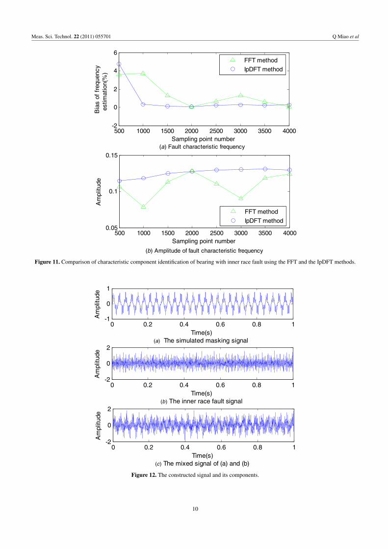
Figure 10(a) shows a comparison of the characteristicfrequency identification of a bearing with an outer race faultusing the FFT and the IpDFT methods, which indicatesthat the IpDFT can accurately identify the outer race faultcharacteristic frequency and provide stable results with smallbias when the number of samples changes from 500 to 4000.However, the FFT method has poor performance comparedwith the IpDFT, and the bias is large for some numbers ofsamples. Figure 10(b) shows a comparison of amplitudeestimation of characteristic frequency, which can representthe severity of an outer race fault. As shown in figure 10(b),the amplitude of the characteristic frequency with the IpDFT issteady, but the amplitude with FFT fluctuates as the number ofsamples changes. Figure 10(b) also shows that the amplitudeof the characteristic component with the IpDFT is larger,which means that the energy leakage of the fault characteristicfrequency is less. Overall, the IpDFT can identify the outerrace fault characteristic frequency and reflect the severity of afault more accurately and steadily than the FFT.

Figure 11 shows a comparison of the characteristiccomponent identification of a bearing with an inner race faultusing the FFT and the IpDFT methods. In figure 11(a), thecharacteristic frequency identification error with the IpDFTat 500 samples is larger than the one with the FFT method,

which is mainly due to the fact that frequency aliasinghappens. However, the IpDFT can identify the inner racefault characteristic frequency accurately and steadily when thenumber of samples changes from 1000 to 4000. Thus, we canget the same conclusion as from figure 10.

4.4. Fault characteristic frequency identification with zoomIpDFT

Most mechanical systems are composed of many elements.The fault characteristic frequency identification we discussedabove is a special case, with the fault in the bearing beingseeded artificially and uniquely (i.e. just one fault at any time).However, multiple faults exist in many mechanical systems,which means that there is a need for multi-fault diagnosis.Furthermore, frequency aliasing arises, and the fault-relatedfrequencies are too close to be effectively distinguished undercertain circumstances. For example, the rotor winding fault isa common failure mode in an induction motor. It is known thatthe rotor winding fault results in an extra current characteristiccomponent with a frequency (1 ± 2 slip ratio) of fundamentalfrequency. Under normal load conditions, the slip ratio is verysmall (a few per cent, even less than one per cent). Therefore,the frequency of the stator fundamental current is very closeto the frequency of the rotor fault current component [18].

If we want to identify two adjacent frequency components,a large number of samples are required to get enough frequencyresolution with the IpDFT or FFT. However, a large numberof points may not always be available due to the restrictions

8

Meas. Sci. Technol. 22 (2011) 055701 Q Miao et al

0 500 1000 15000

0.1

0.2

Frequency(Hz)

Am

plitu

de

0 500 1000 15000

0.1

0.2

Frequency(Hz)

Am

plitu

de

(a) Bearing with inner race fault under 1772 rpm and 1 HP

0 500 1000 15000

0.1

0.2

Frequency(Hz)

Am

plitu

de

(b) Bearing with inner race fault under 1750 rpm and 2 HP

(c) Bearing with inner race fault under 1730 rpm and 3 HP

159.6319.3

157.4 315

309.9155

Figure 9. Identification of characteristic components of bearing with inner race fault in envelope spectra.

500 1000 1500 2000 2500 3000 3500 4000-3

0

3

6

9

12

Bia

s of

frequ

enc

y

estim

atio

n(%

)

Sampling point number

(b) Amplitude of fault characteristic frequency

500 1000 1500 2000 2500 3000 3500 40000.2

0.25

0.3

0.35

0.4

0.45

Am

plitu

de

Sampling point number

(a) Fault characteristic frequency

FFT method

IpDFT method

FFT method

IpDFT method

Figure 10. Comparison of characteristic component identification of bearing with outer race fault using the FFT and the IpDFT methods.

9

Meas. Sci. Technol. 22 (2011) 055701 Q Miao et al

500 1000 1500 2000 2500 3000 3500 4000-2

0

2

4

6

Bia

s of

freq

uen

cy e

stim

atio

n(%

)

Sampling point number

(b) Amplitude of fault characteristic frequency

500 1000 1500 2000 2500 3000 3500 40000.05

0.1

0.15

Am

plitu

de

Sampling point number

(a) Fault characteristic frequency

FFT method

IpDFT method

FFT method

IpDFT method

Figure 11. Comparison of characteristic component identification of bearing with inner race fault using the FFT and the IpDFT methods.

0 0.2 0.4 0.6 0.8 1-1

0

1

Am

plitu

de

Time(s)(a) The simulated masking signal

0 0.2 0.4 0.6 0.8 1-2

0

2

Am

plit

ude

Time(s)(b) The inner race fault signal

0 0.2 0.4 0.6 0.8 1-2

0

2

Am

plitu

de

Time(s)(c) The mixed signal of (a) and (b)

Figure 12. The constructed signal and its components.

10

Meas. Sci. Technol. 22 (2011) 055701 Q Miao et al

150 160 1700

0.05

0.1

0.15

0.2

0.25

Frequency(Hz)

Magnitu

de

150 160 1700

0.05

0.1

0.15

0.2

0.25

Frequency(Hz)

Magnitu

de

150 160 1700

0.05

0.1

0.15

0.2

0.25

Frequency(Hz)

Magnitu

de

158Hz

158.4Hz

162Hz

161.6Hz

(a) FFT (b) Zoom FFT (c) Zoom IpDFT

Figure 13. Comparison of characteristic component identification using the FFT, the zoom FFT and the zoom IpDFT.

of calculation speed and calculation ability for hardware.Theproposed zoom IpDFT in this research is an alternative whendealing with such problems.

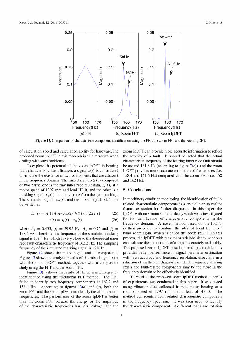
To explore the potential of the zoom IpDFT in bearingfault characteristic identification, a signal x(t) is constructedto simulate the existence of two components that are adjacentin the frequency domain. The mixed signal x(t) is composedof two parts: one is the raw inner race fault data, xi(t), at amotor speed of 1797 rpm and load HP 0, and the other is amasking signal, xm(t), that may come from the gear meshing.The simulated signal, xm(t), and the mixed signal, x(t), canbe written as

xm(t) = A1(1 + A2 cos(2πf2t)) sin(2πf1t) (25)

x(t) = xi(t) + xm(t) (26)

where A1 = 0.435, f1 = 29.95 Hz, A2 = 0.75 and f2 =158.4 Hz. Therefore, the frequency of the simulated maskingsignal is 158.4 Hz, which is very close to the theoretical innerrace fault characteristic frequency of 162.2 Hz. The samplingfrequency of the simulated masking signal is 12 kHz.

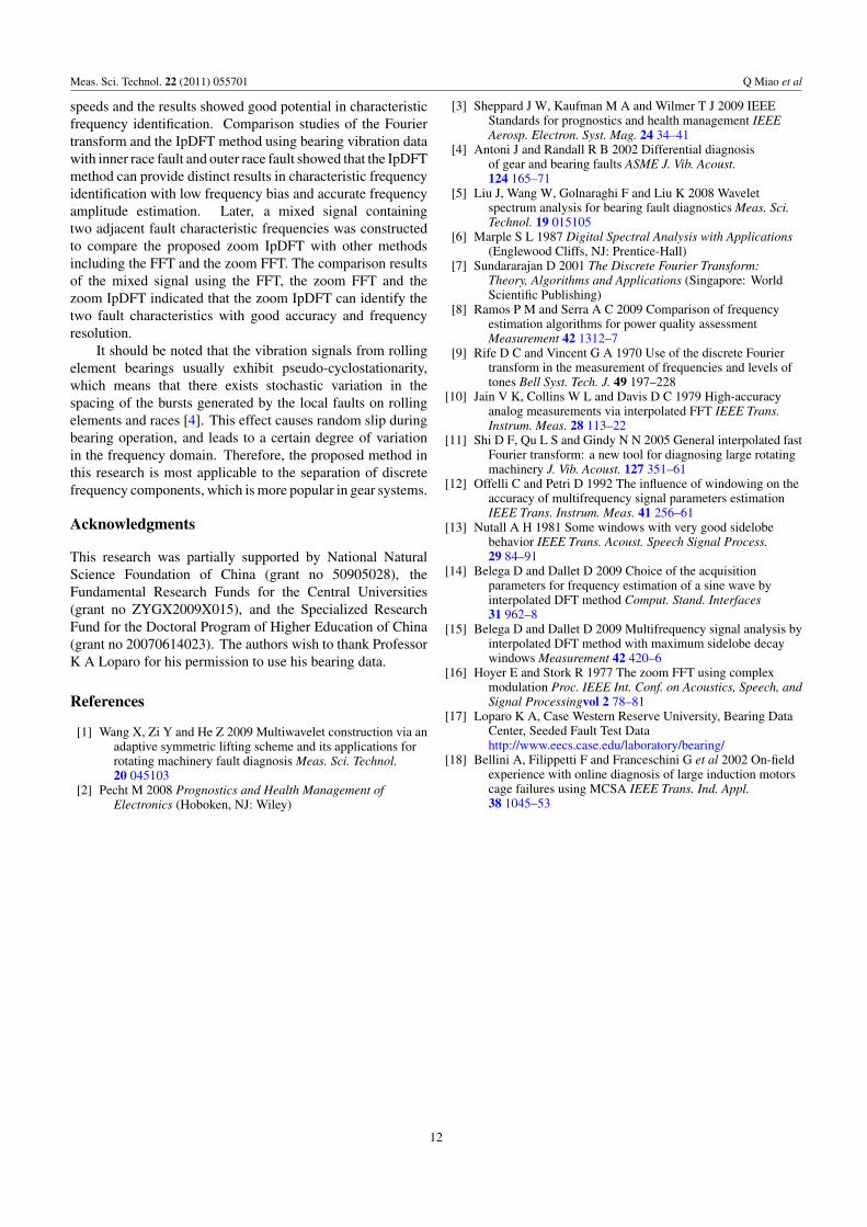
Figure 12 shows the mixed signal and its components.Figure 13 shows the analysis results of the mixed signal x(t)

with the zoom IpDFT method, together with a comparisonstudy using the FFT and the zoom FFT.

Figure 13(a) shows the results of characteristic frequencyidentification using the traditional FFT method. The FFTfailed to identify two frequency components at 162.2 and158.4 Hz. According to figures 13(b) and (c), both thezoom FFT and the zoom IpDFT can identify the characteristicfrequencies. The performance of the zoom IpDFT is betterthan the zoom FFT because the energy or the amplitudeof the characteristic frequencies has less leakage, and the

zoom IpDFT can provide more accurate information to reflectthe severity of a fault. It should be noted that the actualcharacteristic frequency of the bearing inner race fault shouldbe around 161.8 Hz (according to figure 7(c)), and the zoomIpDFT provides more accurate estimation of frequencies (i.e.158.4 and 161.6 Hz) compared with the zoom FFT (i.e. 158and 162 Hz).

5. Conclusions

In machinery condition monitoring, the identification of fault-related characteristic components is a crucial step to realizefeature extraction for further diagnosis. In this paper, theIpDFT with maximum sidelobe decay windows is investigatedfor its identification of characteristic components in thefrequency domain. A novel method based on the IpDFTis then proposed to combine the idea of local frequencyband zooming-in, which is called the zoom IpDFT. In thisprocess, the IpDFT with maximum sidelobe decay windowscan estimate the components of a signal accurately and stably.The proposed zoom IpDFT based on multiple modulationsprovides better performance in signal parameter estimationwith high accuracy and frequency resolution, especially in asituation of multi-fault diagnosis in which frequency aliasingexists and fault-related components may be too close in thefrequency domain to be effectively identified.

To validate the proposed zoom IpDFT method, a seriesof experiments was conducted in this paper. It was testedusing vibration data collected from a motor bearing at arotation speed of 1797 rpm and a load of HP 0. Themethod can identify fault-related characteristic componentsin the frequency spectrum. It was then used to identifythe characteristic components at different loads and rotation

11

Meas. Sci. Technol. 22 (2011) 055701 Q Miao et al

speeds and the results showed good potential in characteristicfrequency identification. Comparison studies of the Fouriertransform and the IpDFT method using bearing vibration datawith inner race fault and outer race fault showed that the IpDFTmethod can provide distinct results in characteristic frequencyidentification with low frequency bias and accurate frequencyamplitude estimation. Later, a mixed signal containingtwo adjacent fault characteristic frequencies was constructedto compare the proposed zoom IpDFT with other methodsincluding the FFT and the zoom FFT. The comparison resultsof the mixed signal using the FFT, the zoom FFT and thezoom IpDFT indicated that the zoom IpDFT can identify thetwo fault characteristics with good accuracy and frequencyresolution.

It should be noted that the vibration signals from rollingelement bearings usually exhibit pseudo-cyclostationarity,which means that there exists stochastic variation in thespacing of the bursts generated by the local faults on rollingelements and races [4]. This effect causes random slip duringbearing operation, and leads to a certain degree of variationin the frequency domain. Therefore, the proposed method inthis research is most applicable to the separation of discretefrequency components, which is more popular in gear systems.

Acknowledgments

This research was partially supported by National NaturalScience Foundation of China (grant no 50905028), theFundamental Research Funds for the Central Universities(grant no ZYGX2009X015), and the Specialized ResearchFund for the Doctoral Program of Higher Education of China(grant no 20070614023). The authors wish to thank ProfessorK A Loparo for his permission to use his bearing data.

References

[1] Wang X, Zi Y and He Z 2009 Multiwavelet construction via anadaptive symmetric lifting scheme and its applications forrotating machinery fault diagnosis Meas. Sci. Technol.20 045103

[2] Pecht M 2008 Prognostics and Health Management ofElectronics (Hoboken, NJ: Wiley)

[3] Sheppard J W, Kaufman M A and Wilmer T J 2009 IEEEStandards for prognostics and health management IEEEAerosp. Electron. Syst. Mag. 24 34–41

[4] Antoni J and Randall R B 2002 Differential diagnosisof gear and bearing faults ASME J. Vib. Acoust.124 165–71

[5] Liu J, Wang W, Golnaraghi F and Liu K 2008 Waveletspectrum analysis for bearing fault diagnostics Meas. Sci.Technol. 19 015105

[6] Marple S L 1987 Digital Spectral Analysis with Applications(Englewood Cliffs, NJ: Prentice-Hall)

[7] Sundararajan D 2001 The Discrete Fourier Transform:Theory, Algorithms and Applications (Singapore: WorldScientific Publishing)

[8] Ramos P M and Serra A C 2009 Comparison of frequencyestimation algorithms for power quality assessmentMeasurement 42 1312–7

[9] Rife D C and Vincent G A 1970 Use of the discrete Fouriertransform in the measurement of frequencies and levels oftones Bell Syst. Tech. J. 49 197–228

[10] Jain V K, Collins W L and Davis D C 1979 High-accuracyanalog measurements via interpolated FFT IEEE Trans.Instrum. Meas. 28 113–22

[11] Shi D F, Qu L S and Gindy N N 2005 General interpolated fastFourier transform: a new tool for diagnosing large rotatingmachinery J. Vib. Acoust. 127 351–61

[12] Offelli C and Petri D 1992 The influence of windowing on theaccuracy of multifrequency signal parameters estimationIEEE Trans. Instrum. Meas. 41 256–61

[13] Nutall A H 1981 Some windows with very good sidelobebehavior IEEE Trans. Acoust. Speech Signal Process.29 84–91

[14] Belega D and Dallet D 2009 Choice of the acquisitionparameters for frequency estimation of a sine wave byinterpolated DFT method Comput. Stand. Interfaces31 962–8

[15] Belega D and Dallet D 2009 Multifrequency signal analysis byinterpolated DFT method with maximum sidelobe decaywindows Measurement 42 420–6

[16] Hoyer E and Stork R 1977 The zoom FFT using complexmodulation Proc. IEEE Int. Conf. on Acoustics, Speech, andSignal Processingvol 2 78–81

[17] Loparo K A, Case Western Reserve University, Bearing DataCenter, Seeded Fault Test Datahttp://www.eecs.case.edu/laboratory/bearing/

[18] Bellini A, Filippetti F and Franceschini G et al 2002 On-fieldexperience with online diagnosis of large induction motorscage failures using MCSA IEEE Trans. Ind. Appl.38 1045–53

12