Dynamic Article LinksC<Journal ofEnvironmentalMonitoringCite this: J. Environ. Monit., 2012, 14, 3037

www.rsc.org/jem PAPER

Publ

ishe

d on

12

Oct

ober

201

2. D

ownl

oade

d by

Hei

nric

h H

eine

Uni

vers

ity o

f D

uess

eldo

rf o

n 20

/11/

2013

14:

58:4

3.

View Article Online / Journal Homepage / Table of Contents for this issue

Identification and modelling the HRT distribution in subsurface constructedwetland

Lijuan Cui,* Yan Zhang, Manyin Zhang, Wei Li, Xinsheng Zhao, Shengnan Li and Yifei Wang

Received 20th February 2012, Accepted 25th September 2012

DOI: 10.1039/c2em30530e

This study focused on the identification of the hydrodynamics of a horizontal subsurface constructed

wetland (HSSF-CW) located in Beijing wildlife rescue and rehabilitation center, Beijing. The effects of

plant growth of iris tectorum on the hydrodynamic behaviours were studied and the distribution of the

hydraulic residence time was simulated by several mathematical models in order to understand the

fluctuations and mixing processes of pollutants in the HSSF-CW. Treatment performance of the HSSF-

CWwas evaluated by comparing the area-based removal rates of different pollutants. According to the

results, water depth has a negative effect on the plant growth and a larger hydraulic loading rate is not

conducive to the growth of wetland plants. Modelling the probability density of the residence time

distribution indicated that the shorter hydraulic residence time of 10.16 hours compared with a

theoretical hydraulic residence time of 12.81 hours was responsible for the lower removal efficiency of

pollutants (T-P: 0.17 � 0.04 g m�2 day�1, T-N: 1.10 � 0.05 g m�2 day�1, PO4–P: 0.08 � 0.04 g m�2

day�1, NH4–N: 0.19 � 0.02 g m�2 day�1, NO3–N: 0.52 � 0.03 g m�2 day�1, Chl_a: 18.26 � 0.09 g m�2

day�1). The results of a superposition simulation of residence time distribution indicated that the

asymmetric double sigmoidal (asym2sig) model is competent at providing a reasonable match between

the measured and the predicted values to some extent. Based on the good fit of the experimental

datasets by the asym2sig probability density function, the mathematical expectation approximated to

the actual hydraulic residence time (10.16 hours) of the HSSF-CW.

Introduction

With the development of the economy, the discharging of

wastewater effluent rich in nitrogen and phosphorus into slow

flowing receiving water bodies such as reservoirs, lakes and

estuaries has led to a number of environmental problems

including eutrophication, which has caused severe impacts on

human health and marine ecology.

Increasingly, wetlands have been recognized as an important

ecosystem with multiple functions such as water storage, flood

Institute of Wetland Research, Chinese Academy of Forestry, HaidianDistrict, Beijing, People’s Republic of China. E-mail: lkyclj@126.com;Fax: +86 010 62824155; Tel: +86 010 62824151

Environmental impact

Research about the characterization of hydrodynamics of CWs he

allow the complicated reaction processes of water flow and deco

operation and quality of discharge water can be accurately calcula

including the hydraulic retention time (HRT) and the flow regime w

and the interaction of plants with water is the main factor to affect t

will contribute to the identification of the optimal HRT and the im

This journal is ª The Royal Society of Chemistry 2012

detention, water purification, nutrient transformation and

ecosystem biodiversity, among which water purification and

pollutant removal have been of great interest to researchers.

Since the treatment processes are efficient, easy to run, ecologi-

cally friendly and low-cost, constructed wetlands (CWs) are

utilized as sustainable alternatives for traditional sewage treat-

ment systems. CW was mainly classified as free water surface

flow constructed wetlands (FWS-CWs) and subsurface flow

constructed wetlands, both of which were widely used for the

purification of wastewater.1

Most of the biological and physicochemical processes in

horizontal subsurface constructed wetlands (HSSF-CWs) are

primarily affected by the comprehensive interactions among

different factors both inside and outside the system such as

lp to reveal the inherent mechanism of sewage treatment, and

mposition of pollutants to be better understood. The design,

ted and evaluated after the characterization of hydrodynamics

as fully understood. Plant growth will change the flow regime

he hydraulic characteristics. Studies on the impact of vegetation

provement of the treatment performance of CWs.

J. Environ. Monit., 2012, 14, 3037–3044 | 3037

Publ

ishe

d on

12

Oct

ober

201

2. D

ownl

oade

d by

Hei

nric

h H

eine

Uni

vers

ity o

f D

uess

eldo

rf o

n 20

/11/

2013

14:

58:4

3.

View Article Online

hydraulic loading rate, distribution of the wetland plants, water

depth and velocity, media matrix, plant species and tempera-

ture.2–5 The hydraulic condition plays an important role in the

maintenance of the function and the construction of HSSF-CWs

and in the determination of species composition. Most of the

synergies largely relying on physical, chemical and biological

processes in the substrates, microorganisms and plant roots

occur within the water flow.6–8

As one of the most important factors influencing the hydraulic

condition of HSSF-CWs, hydraulic retention time is determined

by the mean surface area of the wetland system, water depth and

porosity of the substrate which expresses the space available for

the water to flow through the media, roots and other solids in

CWs.9 Studies revealed that the treatment efficiency of pollutants

in CWs is usually improved by decreasing the hydraulic loading

and the longer the hydraulic retention time, the greater the

nutrient removal.10 The most effective hydraulic retention time is

reported to range from 4 to 15 days,11,12 while research by

Gersberg et al. demonstrated that a short hydraulic retention

time of 3–6 days was effective in removing disease-causing

bacteria and viruses.13

The overall hydrodynamic behaviours of HSSF-CWs are

influenced by the flow variations and the complex internal flow

paths under real operating conditions. Parameters in hydraulic

models addressed the mixing and kinetic characteristics of

HSSF-CWs and tried to explain the complexity of the hydro-

dynamic behaviours combined with many processes involved in

pollution removal.14–16 Research by Werner and Kadlec implied

that internal flows in HSSF-CWs are non-ideal, not fully mixed

and non plug flow, leading to the occurrence of residence time

distribution of a fluid volume.17 Modelling the residence time

distribution of CWs with the assumption of plug flow or

continuously stirred tank reactors (CSTR) was conducted in

previous studies8 and was improved by Kadlec and Wallace.18

However, some specific studies have shown that these ideal

extremes are far from satisfactory. Increasing the complexity of

the simulation model does not correspond to an increase in the

reliability and accuracy.19

Flow patterns of HSSF-CWs are extremely important and the

residence time distribution has been consistently considered as

the key factor affecting the various treatment performances of

HSSF-CWs.17 However, the influence of hydraulic loading rate

on the primary constructed wetland parameters and simulation

of the hydrodynamic behaviors combined with different affecting

factors still require further study. The main objectives of this

study are to show the changes of flow patterns in the HSSF-CW

planted with iris tectorum; to examine the hydrodynamic

behaviors within the HSSF-CW; to evaluate the impact of plant

growth on the hydrodynamic behavior; to evaluate the treatment

performance of the HSSF-CWs during the experimental period.

Materials and method

Description of the study area

This research was conducted in a HSSF-CW located in Beijing

wildlife rescue and rehabilitation center, Shunyi district (Fig. 1).

An artificial lake in this center covered about 1 km2, and was

utilized as the habitat for waterfowl. The artificial lake is half

3038 | J. Environ. Monit., 2012, 14, 3037–3044

enclosed and receives sewage from the cages of wildlife. The open

surface water supplies venues for waterfowl both inside and

outside the center. Underground water is the principal source for

the consistency of the water level. Runoff plays an important

part in the eutrophication of the artificial lake. Frequent activi-

ties and non-interrupted discharge of sewage of different water-

fowl increased the concentration of nutrients in the artificial lake.

Moreover, poor recycle and exchange capacity of the wastewater

combined with nutrients has led to eutrophication problems. The

wetland construction composed of nine FWS-CW units and

three HSSF-CW units was completed in 2008 and was originally

designed to be a comprehensive wetland research and education

facility and was utilized to increase the water quality of the

artificial lake.

Experimental setup

This field experiment was conducted in the middle of September

and in total thirty hours were taken to monitor the hydraulic

behaviors of the HSSF-CW. The total depth of the HSSF-CWs is

0.8 m. Two layers are divided by gravels with different particle

sizes. The bottom layer is filled with 0.3 m depth of gravel, whilst

the upper layer is filled with 0.5 m depth of gravel. Particle sizes

for the bottom and upper layers are 15–30 mm and 5–15 mm

respectively. Ventilation pipes each 10 cm in diameter and 0.10 m

long were embedded to improve the reoxygenation processes in

the HSSF-CW. Density of the ventilation pipes was 1 tube per

m2. The HSSF-CW was dominated by iris tectorum during the

whole experimental period. The applied hydraulic loading rate

was 300 m3 day�1 at the inlet. Plant growth was freely allowed

and the plant density was measured in order to study the inter-

action between plant growth and the hydrodynamic behaviors.

Plant samples were collected from nine plots within the HSSF-

CW (Fig. 2). Each plot was one square metre. Plants in each plot

were harvested at the end of the operating period and charac-

teristics including the plant count, plant density, height, blade

count and diameter, stem and biomass were stated in order to

study the growth of the plants (Table 1). Flow velocity at each

sampling location was measured and triplicate measurements

were recorded.

A tracer study was conducted in order to determine the

hydraulic retention time of the HSSF-CW. The protocol was

based on the rapid injection of 120 L of concentrated sodium

chloride solution at the inlet and the measurement of conduc-

tivity at the outlet (100 mg L�1).

The treatment performance of the HSSF-CW has been

monitored since the operation began. Water samples at the inlet

and outlet have been collected every two hours throughout the

operating period. Triplicate wastewater samples at each

sampling point were analyzed to determine the water quality.

Water samples were kept at 4 �C and later filtered through

millipore membrane filters (0.45 mm) for the subsequent

measurements of nutrients. The YSI 6-series sonde was used to

monitor parameters including temperature, dissolved oxygen,

pH and turbidity at sample locations. Samples were analyzed for

total phosphorus (T-P), orthophosphate (PO4–P), total nitrogen

(T-N), nitrate nitrogen (NO3–N), ammonia (NH4–N), and

chlorophyll a (Chl_a) in accordance with the standard

methods.20

This journal is ª The Royal Society of Chemistry 2012

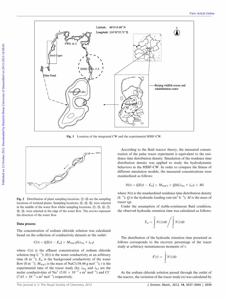
Fig. 1 Location of the integrated CW and the experimental HSSF-CW.

Fig. 2 Distribution of plant sampling locations. ①–⑨ are the sampling

locations of wetland plants. Sampling locations, ②, ⑤, ⑥, were selected

in the middle of the water flow whilst sampling locations, ①, ③, ④, ⑦,

⑧, ⑨, were selected at the edge of the water flow. The arrows represent

the direction of the water flow.

Publ

ishe

d on

12

Oct

ober

201

2. D

ownl

oade

d by

Hei

nric

h H

eine

Uni

vers

ity o

f D

uess

eldo

rf o

n 20

/11/

2013

14:

58:4

3.

View Article Online

Data process

The concentration of sodium chloride solution was calculated

based on the collection of conductivity datasets at the outlet:

C(t) ¼ ([E(t) � Ew] � MNaCl)/(lNa + lCl)

where C(t) is the effluent concentration of sodium chloride

solution (mg L�1); E(t) is the water conductivity at an arbitrary

time (S m�1); Ew is the background conductivity of the water

flow (S m�1); MNaCl is the mass of NaCl (58.44 g mol�1); t is the

experimental time of the tracer study (h); lNa and lCl are the

molar conductivities of Na+ (5.01 � 10�3 s m2 mol�1) and Cl�

(7.63 � 10�3 s m2 mol�1) respectively.

This journal is ª The Royal Society of Chemistry 2012

According to the fluid reactor theory, the measured concen-

tration of the pulse tracer experiment is equivalent to the resi-

dence time distribution density. Simulation of the residence time

distribution density was applied to study the hydrodynamic

behaviors in the HSSF-CW. In order to compare the fitness of

different simulation models, the measured concentrations were

standardized as follows:

N(t) ¼ ([E(t) � Ew] � MNaCl � Q)/((lNa + lCl) � M)

whereN(t) is the standardized residence time distribution density

(h�1); Q is the hydraulic loading rate (m3 h�1); M is the mass of

tracer (g).

Under the assumption of stable-continuous fluid condition,

the observed hydraulic retention time was calculated as follows:

Tm ¼ðN0

NðtÞtdt,ðN

0

NðtÞdt

The distribution of the hydraulic retention time presented as

follows corresponds to the recovery percentage of the tracer

study at arbitrary instantaneous moments of t:

FðtÞ ¼ðt0

NðtÞdt

As the sodium chloride solution passed through the outlet of

the reactor, the variation of the tracer study (s) was calculated by

J. Environ. Monit., 2012, 14, 3037–3044 | 3039

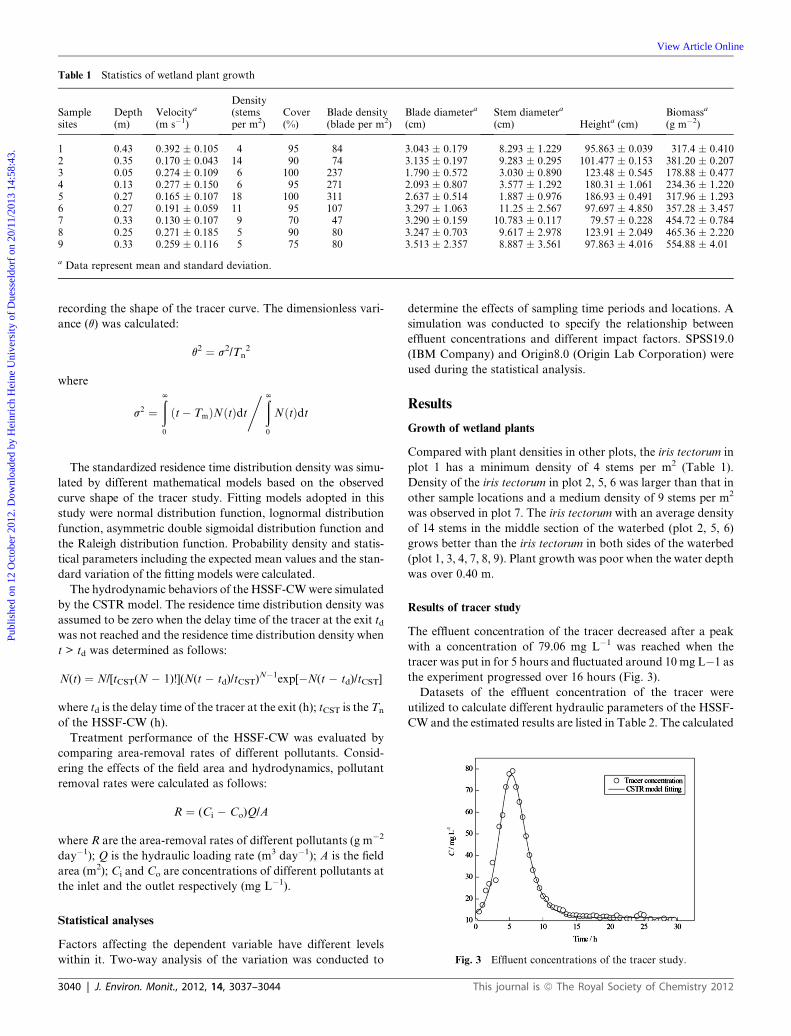
Table 1 Statistics of wetland plant growth

Samplesites

Depth(m)

Velocitya

(m s�1)

Density(stemsper m2)

Cover(%)

Blade density(blade per m2)

Blade diametera

(cm)Stem diametera

(cm) Heighta (cm)Biomassa

(g m�2)

1 0.43 0.392 � 0.105 4 95 84 3.043 � 0.179 8.293 � 1.229 95.863 � 0.039 317.4 � 0.4102 0.35 0.170 � 0.043 14 90 74 3.135 � 0.197 9.283 � 0.295 101.477 � 0.153 381.20 � 0.2073 0.05 0.274 � 0.109 6 100 237 1.790 � 0.572 3.030 � 0.890 123.48 � 0.545 178.88 � 0.4774 0.13 0.277 � 0.150 6 95 271 2.093 � 0.807 3.577 � 1.292 180.31 � 1.061 234.36 � 1.2205 0.27 0.165 � 0.107 18 100 311 2.637 � 0.514 1.887 � 0.976 186.93 � 0.491 317.96 � 1.2936 0.27 0.191 � 0.059 11 95 107 3.297 � 1.063 11.25 � 2.567 97.697 � 4.850 357.28 � 3.4577 0.33 0.130 � 0.107 9 70 47 3.290 � 0.159 10.783 � 0.117 79.57 � 0.228 454.72 � 0.7848 0.25 0.271 � 0.185 5 90 80 3.247 � 0.703 9.617 � 2.978 123.91 � 2.049 465.36 � 2.2209 0.33 0.259 � 0.116 5 75 80 3.513 � 2.357 8.887 � 3.561 97.863 � 4.016 554.88 � 4.01

a Data represent mean and standard deviation.

Publ

ishe

d on

12

Oct

ober

201

2. D

ownl

oade

d by

Hei

nric

h H

eine

Uni

vers

ity o

f D

uess

eldo

rf o

n 20

/11/

2013

14:

58:4

3.

View Article Online

recording the shape of the tracer curve. The dimensionless vari-

ance (q) was calculated:

q2 ¼ s2/Tn2

where

s2 ¼ðN0

ðt� TmÞNðtÞdt,ðN

0

NðtÞdt

The standardized residence time distribution density was simu-

lated by different mathematical models based on the observed

curve shape of the tracer study. Fitting models adopted in this

study were normal distribution function, lognormal distribution

function, asymmetric double sigmoidal distribution function and

the Raleigh distribution function. Probability density and statis-

tical parameters including the expected mean values and the stan-

dard variation of the fitting models were calculated.

The hydrodynamic behaviors of the HSSF-CWwere simulated

by the CSTR model. The residence time distribution density was

assumed to be zero when the delay time of the tracer at the exit tdwas not reached and the residence time distribution density when

t > td was determined as follows:

N(t) ¼ N/[tCST(N � 1)!](N(t � td)/tCST)N�1exp[�N(t � td)/tCST]

where td is the delay time of the tracer at the exit (h); tCST is the Tn

of the HSSF-CW (h).

Treatment performance of the HSSF-CW was evaluated by

comparing area-removal rates of different pollutants. Consid-

ering the effects of the field area and hydrodynamics, pollutant

removal rates were calculated as follows:

R ¼ (Ci � Co)Q/A

where R are the area-removal rates of different pollutants (g m�2

day�1); Q is the hydraulic loading rate (m3 day�1); A is the field

area (m2); Ci and Co are concentrations of different pollutants at

the inlet and the outlet respectively (mg L�1).

Fig. 3 Effluent concentrations of the tracer study.

Statistical analyses

Factors affecting the dependent variable have different levels

within it. Two-way analysis of the variation was conducted to

3040 | J. Environ. Monit., 2012, 14, 3037–3044

determine the effects of sampling time periods and locations. A

simulation was conducted to specify the relationship between

effluent concentrations and different impact factors. SPSS19.0

(IBM Company) and Origin8.0 (Origin Lab Corporation) were

used during the statistical analysis.

Results

Growth of wetland plants

Compared with plant densities in other plots, the iris tectorum in

plot 1 has a minimum density of 4 stems per m2 (Table 1).

Density of the iris tectorum in plot 2, 5, 6 was larger than that in

other sample locations and a medium density of 9 stems per m2

was observed in plot 7. The iris tectorum with an average density

of 14 stems in the middle section of the waterbed (plot 2, 5, 6)

grows better than the iris tectorum in both sides of the waterbed

(plot 1, 3, 4, 7, 8, 9). Plant growth was poor when the water depth

was over 0.40 m.

Results of tracer study

The effluent concentration of the tracer decreased after a peak

with a concentration of 79.06 mg L�1 was reached when the

tracer was put in for 5 hours and fluctuated around 10 mg L�1 as

the experiment progressed over 16 hours (Fig. 3).

Datasets of the effluent concentration of the tracer were

utilized to calculate different hydraulic parameters of the HSSF-

CW and the estimated results are listed in Table 2. The calculated

This journal is ª The Royal Society of Chemistry 2012

Publ

ishe

d on

12

Oct

ober

201

2. D

ownl

oade

d by

Hei

nric

h H

eine

Uni

vers

ity o

f D

uess

eldo

rf o

n 20

/11/

2013

14:

58:4

3.

View Article Online

discharge for the HSSF-CW was 103.04 m3 h�1. Based on the

observation of the answer curve obtained from the tracer study,

the nominal hydraulic retention time was 12.81 hours whilst the

actual hydraulic retention time was 10.16 hours.

The residence time distribution density of the HSSF-CW was

simulated by different distribution functions in this study.

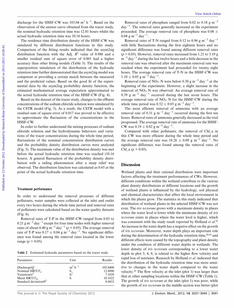
Comparison of the fitting results indicated that the asym2sig

distribution function with the Adj. R2 value of 0.988 and a

smaller residual sum of square error of 0.001 had a higher

accuracy than other fitting models (Table 3). The results of the

superposition simulation of the distribution of the hydraulic

retention time further demonstrated that the asym2sig model was

competent at providing a certain match between the measured

and the predicted values. Based on the good fit of the experi-

mental data by the asym2sig probability density function, the

estimated mathematical average expectation approximated to

the actual hydraulic retention time of the HSSF-CW (Fig. 4).

Based on the dataset of the tracer study, changes to the effluent

concentrations of the sodium chloride solution were simulated by

the CSTR model (Fig. 3). As a result, the CSTR model with a

residual sum of square error of 0.017 was proved to be effective

to approximate the fluctuation of the concentrations in the

HSSF-CW.

In order to further understand the mixing processes of sodium

chloride solution and the hydrodynamic behaviors and varia-

tions of the tracer concentrations during the whole time period,

fluctuations of the nominal concentration distribution curves

and the probability density distribution curves were analyzed

(Fig. 5). The maximum value of the distribution density was met

before the actual hydraulic retention time was reached (10.16

hours). A general fluctuation of the probability density distri-

bution with a tailing phenomenon after a steep relief was

observed. The distribution function was calculated as 0.65 at the

point of the actual hydraulic retention time.

Treatment performance

In order to understand the removal processes of different

pollutants, water samples were collected at the inlet and outlet

every two hours during the whole time period and removal rates

of pollutants were calculated based on the water quality datasets

(Fig. 6).

Removal rates of T-P in the HSSF-CW ranged from 0.03 to

0.21 g m�2 day�1 except for four time nodes with higher removal

rates of about 0.40 g m�2 day�1 (p < 0.05). The average removal

rate of T-P was 0.17 � 0.04 g m�2 day�1. No significant differ-

ence was found among the removal rates located in the lower

range (p > 0.05).

Table 2 Estimated hydraulic parameters based on the tracer study

Parameters Unit Results

Discharge/Q m3 h�1 103.0400Nominal HRT/Tn h 12.8090Variation/s2 h2 7.1039Mean HRT/Tm h 10.1622Standard deviation/q2 0.0433

This journal is ª The Royal Society of Chemistry 2012

Removal rates of phosphate ranged from 0.02 to 0.18 g m�2

day�1. The removal rates generally increased as the experiment

proceeded. The average removal rate of phosphate was 0.08 �0.04 g m�2 day�1.

Removal rates of T-N ranged from 0.12 to 0.96 g m�2 day�1

with little fluctuations during the first eighteen hours and no

significant difference was found among different removal rates

(p > 0.05). However, removal rates increased from 1.21 to 3.19 g

m�2 day�1 during the last twelve hours and a little decrease in the

removal rate was observed after the maximum removal rate was

reached when the experiment had proceeded for twenty eight

hours. The average removal rate of T-N in the HSSF-CW was

1.10 � 0.05 g m�2 day�1.

Removal rates of NO3–N were below 0.30 g m�2 day�1 at the

beginning of the experiment. However, a slight increase in the

removal of NO3–N was observed. An average removal rate of

0.39 g m�2 day�1 occurred during the last seven hours. The

average removal rate of NO3–N for the HSSF-CW during the

whole time period was 0.52 � 0.03 g m�2 day�1.

The most efficient removal of ammonia with an average

removal rate of 0.31 g m�2 day�1 occurred during the first ten

hours. Removal rates of ammonia generally decreased as the trial

progressed. The average removal rate of ammonia for the HSSF-

CW was 0.19 � 0.02 g m�2 day�1.

Compared with other pollutants, the removal of Chl_a in

this CW was more efficient during the whole time period and

the average removal rate was 18.26 � 0.09 g m�2 day�1. No

significant difference was found among the removal rates of

Chl_a (p > 0.05).

Discussion

Wetland plants and their rational distribution were important

factors affecting the treatment performances of CWs. However,

different conditions within the wetland contribute to the various

plant density distributions at different locations and the growth

of wetland plants is influenced by the hydrology, soil physical

and chemical characteristics that affect the local environment in

which the plants grow. The statistics in this study indicated that

distribution of wetland plants in the selected HSSF-CW was not

even. The iris tectorum grows with a maximum density in places

where the water level is lower while the minimum density of iris

tectorum exists in places where the water level is higher, which

was consistent with the study result reported by Holland et al.21

An increase in the water depth has a negative effect on the growth

of iris tectorum. Moreover, water depth plays an important role

during the determination of the hydraulic retention time,22,23 and

different effects were caused by the topography and plant density

under the condition of different water depths in wetlands. The

lower density of iris tectorum corresponding to a lower water

depth in plot 3, 4, 8, is related to the higher flow velocity and

rapid loss of nutrients. Research by Holland et al. indicated that

the distribution of the hydraulic retention time was more sensi-

tive to changes in the water depth compared to the water

velocity.21 The flow velocity at the inlet (plot 1) was larger than

that at other sampling locations within the HSSF-CW (Table 1).

The growth of iris tectorum at the inlet (plot 1) was poor, while

the growth of iris tectorum in the middle section was better (plot

J. Environ. Monit., 2012, 14, 3037–3044 | 3041

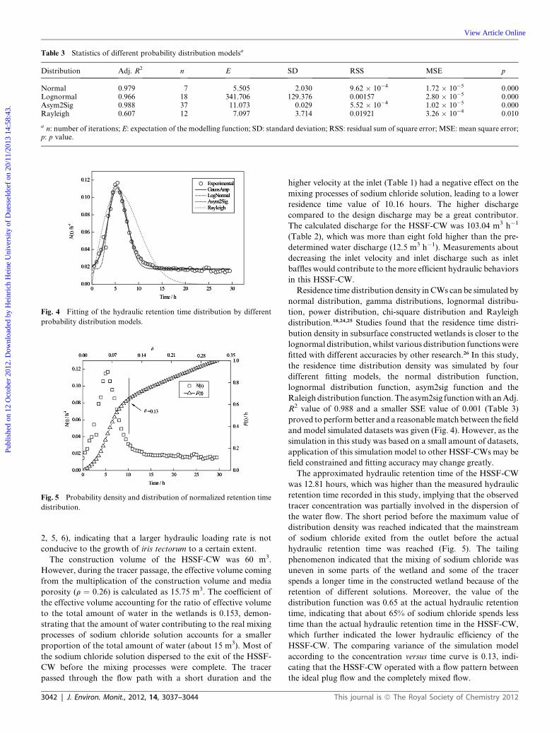
Table 3 Statistics of different probability distribution modelsa

Distribution Adj. R2 n E SD RSS MSE p

Normal 0.979 7 5.505 2.030 9.62 � 10�4 1.72 � 10�5 0.000Lognormal 0.966 18 341.706 129.376 0.00157 2.80 � 10�5 0.000Asym2Sig 0.988 37 11.073 0.029 5.52 � 10�4 1.02 � 10�5 0.000Rayleigh 0.607 12 7.097 3.714 0.01921 3.26 � 10�4 0.010

a n: number of iterations; E: expectation of the modelling function; SD: standard deviation; RSS: residual sum of square error; MSE: mean square error;p: p value.

Fig. 4 Fitting of the hydraulic retention time distribution by different

probability distribution models.

Fig. 5 Probability density and distribution of normalized retention time

distribution.

Publ

ishe

d on

12

Oct

ober

201

2. D

ownl

oade

d by

Hei

nric

h H

eine

Uni

vers

ity o

f D

uess

eldo

rf o

n 20

/11/

2013

14:

58:4

3.

View Article Online

2, 5, 6), indicating that a larger hydraulic loading rate is not

conducive to the growth of iris tectorum to a certain extent.

The construction volume of the HSSF-CW was 60 m3.

However, during the tracer passage, the effective volume coming

from the multiplication of the construction volume and media

porosity (r ¼ 0.26) is calculated as 15.75 m3. The coefficient of

the effective volume accounting for the ratio of effective volume

to the total amount of water in the wetlands is 0.153, demon-

strating that the amount of water contributing to the real mixing

processes of sodium chloride solution accounts for a smaller

proportion of the total amount of water (about 15 m3). Most of

the sodium chloride solution dispersed to the exit of the HSSF-

CW before the mixing processes were complete. The tracer

passed through the flow path with a short duration and the

3042 | J. Environ. Monit., 2012, 14, 3037–3044

higher velocity at the inlet (Table 1) had a negative effect on the

mixing processes of sodium chloride solution, leading to a lower

residence time value of 10.16 hours. The higher discharge

compared to the design discharge may be a great contributor.

The calculated discharge for the HSSF-CW was 103.04 m3 h�1

(Table 2), which was more than eight fold higher than the pre-

determined water discharge (12.5 m3 h�1). Measurements about

decreasing the inlet velocity and inlet discharge such as inlet

baffles would contribute to the more efficient hydraulic behaviors

in this HSSF-CW.

Residence time distribution density inCWs can be simulated by

normal distribution, gamma distributions, lognormal distribu-

tion, power distribution, chi-square distribution and Rayleigh

distribution.18,24,25 Studies found that the residence time distri-

bution density in subsurface constructed wetlands is closer to the

lognormal distribution, whilst various distribution functionswere

fitted with different accuracies by other research.26 In this study,

the residence time distribution density was simulated by four

different fitting models, the normal distribution function,

lognormal distribution function, asym2sig function and the

Raleigh distribution function. The asym2sig functionwith anAdj.

R2 value of 0.988 and a smaller SSE value of 0.001 (Table 3)

proved to performbetter and a reasonablematchbetween the field

and model simulated datasets was given (Fig. 4). However, as the

simulation in this study was based on a small amount of datasets,

application of this simulation model to other HSSF-CWs may be

field constrained and fitting accuracy may change greatly.

The approximated hydraulic retention time of the HSSF-CW

was 12.81 hours, which was higher than the measured hydraulic

retention time recorded in this study, implying that the observed

tracer concentration was partially involved in the dispersion of

the water flow. The short period before the maximum value of

distribution density was reached indicated that the mainstream

of sodium chloride exited from the outlet before the actual

hydraulic retention time was reached (Fig. 5). The tailing

phenomenon indicated that the mixing of sodium chloride was

uneven in some parts of the wetland and some of the tracer

spends a longer time in the constructed wetland because of the

retention of different solutions. Moreover, the value of the

distribution function was 0.65 at the actual hydraulic retention

time, indicating that about 65% of sodium chloride spends less

time than the actual hydraulic retention time in the HSSF-CW,

which further indicated the lower hydraulic efficiency of the

HSSF-CW. The comparing variance of the simulation model

according to the concentration versus time curve is 0.13, indi-

cating that the HSSF-CW operated with a flow pattern between

the ideal plug flow and the completely mixed flow.

This journal is ª The Royal Society of Chemistry 2012

Fig. 6 Removal rates of different pollutants in the HSSF-CW.

Publ

ishe

d on

12

Oct

ober

201

2. D

ownl

oade

d by

Hei

nric

h H

eine

Uni

vers

ity o

f D

uess

eldo

rf o

n 20

/11/

2013

14:

58:4

3.

View Article Online

Phosphate minerals in sediments and assimilation of biomass

were the main phosphorus removal mechanisms in wetland

environments. Degradation by parts of plant tissues probably

improves the phosphorus removal efficiency. Processes such as

mineral precipitation, ion exchange, adsorption that conduct on

the planted bed were also responsible for the removal of phos-

phorus within a certain time. During most of the time periods in

the present study, the lower removal rates of phosphorus indi-

cated that phosphorus removal by the HSSF-CW was not effi-

cient. The amount of phosphorus adsorption by plants was

limited under a high background concentration and removals are

likely to decrease over time due to the saturation of phosphorus

sorption sites in the medium.27–29 Wetland plants play an

important role in the removal of soluble phosphate. The main

stochastic process responsible for the removal of dissolved

and non-dissolved phosphate was biological absorption, while

This journal is ª The Royal Society of Chemistry 2012

phosphate transportation between the sediment pore water and

the surface water through adsorption and desorption processes

balances the amount of phosphates at different compositions of

the HSSF-CW. The increasing absorption and utilization by

wetland plants is also a contributory factor to the increasing

removal rates of soluble phosphate.

The major processes responsible for nitrogen removal in

constructed wetlands were adsorption, assimilation into micro-

bial and plant biomass, ammonia volatilization and coupled

nitrification–denitrification. T-N was assimilated and utilized in

the metabolism processes of emergent and submerged plants with

a high velocity at the growth seasons.30 However, the amount of

T-N removed by plants was not recorded in this study. The

absorption of nitrogen by wetland plants from the water body

and sediments was rapid at growth seasons. Removal of nitrates

by the HSSF-CW generally increased during the whole period

J. Environ. Monit., 2012, 14, 3037–3044 | 3043

Publ

ishe

d on

12

Oct

ober

201

2. D

ownl

oade

d by

Hei

nric

h H

eine

Uni

vers

ity o

f D

uess

eldo

rf o

n 20

/11/

2013

14:

58:4

3.

View Article Online

(Fig. 6). The lower oxygen level and rich carbon reservation

under the water surface covered with wetland plants may be

responsible for the higher velocity of denitrification that trans-

formed nitrates to nitrogen and nitrous oxide. Transformation of

the organic nitrogen into ammonia happened both in aerobic and

anaerobic environments. Reverse conclusions focusing on the

role of oxygen in the transformation processes were found in

previous studies.7,31 The pH and temperature were important

factors which influenced the reactive velocity. The pH value of

7.93 � 1.40 in this study probably contributed to the low vola-

tilization of ammonia in the constructed wetland and the

removal rates generally decreased as the experiment proceeded.

However, the lower concentration of dissolved oxygen in water

around dense plants and the stable carbon supplement from

aging and decaying plant tissues make a suitable condition for

the denitrification process, which was proven to be the most

important removal process for T-N.32

Changes in the patterns of Chl_a are relative to P levels in a

P-limited system with heavy grazing of phytoplankton by inverte-

brates. In this study, a two-tailed test of significance is applied at the

significant level of 0.05 to perform the correlation analysis between

the T-P removal rates and Chl_a removal rates. The Pearson

coefficient value was 0.46 (p ¼ 0.07), indicating a weak positive

relationshipbetween the twovariables.Under the conceptionof the

weak correlations, increased grazing by zooplankton may be

partially responsible for the decrease of total phosphorus recorded

in this study. However, the limiting factors for the treatment

performances of the HSSF-CW need further study.

Conclusions

The higher hydraulic loading rate in this HSSF-CW was not

conducive to the growth of iris tectorum. Simulation of the tracer

study revealed a lower hydraulic efficiency of the HSSF-CW and

fitting of the residence time distribution density indicated that the

asym2sig model was competent at providing a better match

between the experimental and field datasets to a certain extent.

Acknowledgements

This study was funded by the Taihu Lake Wetland Ecosystem

Function Mechanism and Regulation Techniques (200904001)

projects. We thank Gao Changjun and Ma Qiongfang for

assistance with wastewater sampling and collection of field data.

We are also grateful to all members of the research team for their

helpful comments and advice.

3044 | J. Environ. Monit., 2012, 14, 3037–3044

References

1 J. Vymazal, Ecol. Eng., 2009, 35, 1–17.2 R. S. Jadhav and S. G. Buchberger, Ecol. Eng., 1995, 5, 481–496.3 A. D. Karathanasis, C. L. Potter and M. S. Coyne, Ecol. Eng., 2003,20, 157–169.

4 C. S. Akratos and V. A. Tsihrintzis, Ecol. Eng., 2007, 29, 173–191.5 N. T. D. Trang, D. Konnerup, H.-H. Schierup, N. H. Chiem,L. A. Tuan and H. Brix, Ecol. Eng., 2010, 36, 527–535.

6 D. Giraldi, M. de’Michieli Vitturi, M. Zaramella, A. Marion andR. Iannelli, Ecol. Eng., 2009, 35, 265–273.

7 L. Hu, W. Hu, J. Deng, Q. Li, F. Gao, J. Zhu and T. Han, Ecol. Eng.,2010, 36, 1725–1732.

8 F. Chazarenc, G. Merlin and Y. Gonthier, Ecol. Eng., 2003, 21, 165–173.

9 S. C. Reed, R. W. Crites and E. J. Middlebrooks, Natural Systems forWaste Management and Treatment, McGraw-Hill Professional, 1998.

10 K. Sakadevan and H. J. Bavor, Water Sci. Technol., 1999, 40, 121–128.

11 G. Tchobanoglous, F. L. Burton and H. D. Stensel, WastewaterEngineering: Treatment and Reuse, McGraw-Hill Science/Engineering/Math, 2003.

12 J. Watson and J. Hobson, Constructed Wetlands for WastewaterTreatment: Municipal, Industrial and Agricultural, Lewis Publishers,Chelsea Michigan, 1989, pp. 379–391, 9 fig, 12 ref., 1989.

13 R. M. Gersberg, R. A. Gearheart and M. Ives, Constructed Wetlandsfor Wastewater Treatment: Municipal, Industrial and Agricultural,Lewis Publishers, Chelsea Michigan, 1989, pp. 431–445, 5 fig, 4 tab,42 ref., 1989.

14 S. G. Buchberger and G. B. Shaw, Ecol. Eng., 1995, 4, 249–275.15 S. Marsili-Libelli and N. Checchi, Ecol. Eng., 2005, 187, 201–218.16 T. M. Wynn and S. K. Liehr, Ecol. Eng., 2001, 16, 519–536.17 T.M.Werner and R. H. Kadlec, Ecological Engineering, 2000, 15, 77–

90.18 R. H. Kadlec and S. Wallace, Treatment Wetlands, CRC, 2009.19 D. P. L. Rousseau, P. A. Vanrolleghem and N. De Pauw,Water Res.,

2004, 38, 1484–1493.20 M. J. Taras, Standard Methods for the Examination of Water and

Wastewater, American Public Health Association, 1971.21 J. F. Holland, J. F. Martin, T. Granata, V. Bouchard, M. Quigley and

L. Brown, Ecol. Eng., 2004, 23, 189–203.22 B. A. Middleton, Aquat. Bot., 1990, 37, 189–196.23 D. A. Wilcox and Y. Xie, J. Great Lakes Res., 2007, 33, 751–773.24 A. W€orman and V. Kronn€as, J. Hydrol., 2005, 301, 123–138.25 A. W€orman, A. I. Packman, L. Marklund, J. W. Harvey and

S. H. Stone, Geophys. Res. Lett., 2007, 34, L07402.26 Y. You, Y. Ma, W. Bao and J. Hu, China Rural Water and

Hydropower, 2008, 3, 36–43.27 C. A. Arias, M. Del Bubba and H. Brix, WaterRes., 2001, 35, 1159–

1168.28 C. A. Arias and H. Brix, Water Sci. Technol., 2005, 51, 267–274.29 C. Vohla, R. Alas, K. Nurk, S. Baatz and €U. Mander, Sci. Total

Environ., 2007, 380, 66–74.30 D. O. Huett, S. G. Morris, G. Smith and N. Hunt, Water Res., 2005,

39, 3259–3272.31 J. G. Allen, M. W. Beutel, D. R. Call and A. M. Fischer, Bioresour.

Technol., 2010, 101, 1389–1392.32 R. H. Kadlec and R. L. Knight, Treatment Wetlands, CRC, 1996.

This journal is ª The Royal Society of Chemistry 2012