Nonlinear Analysis: Hybrid Systems 5 (2011) 446–456

Contents lists available at ScienceDirect

Nonlinear Analysis: Hybrid Systems

journal homepage: www.elsevier.com/locate/nahs

Identification and estimation of parameters defining a class ofhybrid systemsSandeep Dhar, Swaroop Darbha, K.R. Rajagopal ∗Department of Mechanical Engineering, Texas A&M University, College Station, TX 77843, USA

a r t i c l e i n f o

Article history:Received 13 March 2010Accepted 8 April 2010

Keywords:Sequential hybrid systemsParameter estimationMulti-modal systemsAir brakeDiagnostics

a b s t r a c t

In this paper, we consider the problem of parameter estimation in an air brake system.In an air brake system, the pressure of air in the brake chamber and the displacement ofthe pushrod and their derivatives form a set of states that characterize the system. Theposition of a valve or mass flow rate of air is an input and the pressure is the measuredvariable or the output. The pressure acting on the pushrod of the brake chamber causesmotion, and the mode in which the system operates depends on the displacement of thepushrod. The mode-dependent nature of the system is a result of different sets of springcompliances associated with the piston in different ranges of its displacement. The modetomode transition in the air brake system is governedby aparameterwhich is the clearancebetween the brake pads and the drum. The clearance between the brake pads and thedrum can vary due to a variety of factors — for example, brake pad wear or brake fade. Inthese applications, characterizing the transition from onemode to another requires a lot ofconstitutive assumptions, and it can be difficult to calibrate the parameters associatedwiththe constitutive assumptions. We therefore treat the air brake system as a system in whichthe parameter governing the transition from one mode to another (clearance between thebrake pads and the drum) is not known exactly. Clearly, this parameter dictates the timedelay and lag between the command and delivery of the brake torque at the wheels andaffects the stopping distance of the vehicles considerably. The problem of identificationconsidered in this paper is as follows. Suppose that the pressure of the fluid were to bemeasured and that the motion of the piston is not measured. Is it possible to estimate thefinal displacement of the piston without knowing the parameters that govern the system totransition from one mode to another?

© 2010 Elsevier Ltd. All rights reserved.

1. Introduction

Many phenomena that are observed in nature as well as those that are a consequence of technological developments arehybrid systems. The classic problem of friction is one wherein the equations governing the static state of a body are quitedifferent from those governing its dynamics. The term ‘‘hybrid’’ canmean different things to different researchers. For thosemodeling the response of metals duringmelting and solidification of metals, a phase change can not only induce a change insymmetry of thematerial response but also result in different governing differential equations (including partial differentialequations of different orders) depending on the constitutive assumptions concerning the response of the material; forexample, modeling the problem of fiber spinning given in [1] leads to a hybrid system, wherein the different modes aregoverned by distinct systems of partial differential equations. In this paper, we will consider far more restrictive hybridsystems, such as those that arise in an engineering application such as that governing the dynamics of air brakes in trucks,wherein we have different ordinary differential equations governing the different modes.

∗ Corresponding author. Tel.: +1 979 862 4552.E-mail addresses: sandeep_dhar@tamu.edu (S. Dhar), dswaroop@tamu.edu (S. Darbha), krajagopal@tamu.edu (K.R. Rajagopal).

1751-570X/$ – see front matter© 2010 Elsevier Ltd. All rights reserved.doi:10.1016/j.nahs.2010.04.001

S. Dhar et al. / Nonlinear Analysis: Hybrid Systems 5 (2011) 446–456 447

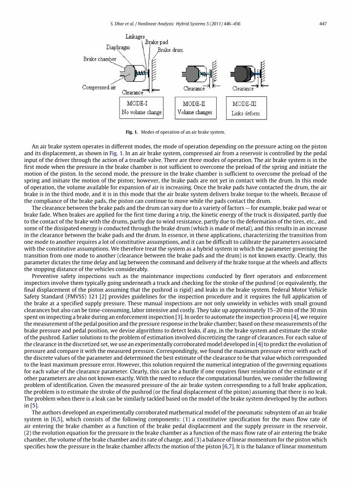
Fig. 1. Modes of operation of an air brake system.

An air brake system operates in different modes, the mode of operation depending on the pressure acting on the pistonand its displacement, as shown in Fig. 1. In an air brake system, compressed air from a reservoir is controlled by the pedalinput of the driver through the action of a treadle valve. There are three modes of operation. The air brake system is in thefirst mode when the pressure in the brake chamber is not sufficient to overcome the preload of the spring and initiate themotion of the piston. In the second mode, the pressure in the brake chamber is sufficient to overcome the preload of thespring and initiate the motion of the piston; however, the brake pads are not yet in contact with the drum. In this modeof operation, the volume available for expansion of air is increasing. Once the brake pads have contacted the drum, the airbrake is in the third mode, and it is in this mode that the air brake system delivers brake torque to the wheels. Because ofthe compliance of the brake pads, the piston can continue to move while the pads contact the drum.

The clearance between the brake pads and the drum can vary due to a variety of factors — for example, brake padwear orbrake fade. When brakes are applied for the first time during a trip, the kinetic energy of the truck is dissipated, partly dueto the contact of the brake with the drums, partly due to wind resistance, partly due to the deformation of the tires, etc., andsome of the dissipated energy is conducted through the brake drum (which is made of metal), and this results in an increasein the clearance between the brake pads and the drum. In essence, in these applications, characterizing the transition fromonemode to another requires a lot of constitutive assumptions, and it can be difficult to calibrate the parameters associatedwith the constitutive assumptions. We therefore treat the system as a hybrid system in which the parameter governing thetransition from one mode to another (clearance between the brake pads and the drum) is not known exactly. Clearly, thisparameter dictates the time delay and lag between the command and delivery of the brake torque at the wheels and affectsthe stopping distance of the vehicles considerably.

Preventive safety inspections such as the maintenance inspections conducted by fleet operators and enforcementinspectors involve them typically going underneath a truck and checking for the stroke of the pushrod (or equivalently, thefinal displacement of the piston assuming that the pushrod is rigid) and leaks in the brake system. Federal Motor VehicleSafety Standard (FMVSS) 121 [2] provides guidelines for the inspection procedure and it requires the full application ofthe brake at a specified supply pressure. These manual inspections are not only unwieldy in vehicles with small groundclearances but also can be time-consuming, labor intensive and costly. They take up approximately 15–20min of the 30minspent on inspecting a brake during an enforcement inspection [3]. In order to automate the inspection process [4], we requirethemeasurement of the pedal position and the pressure response in the brake chamber; based on thesemeasurements of thebrake pressure and pedal position, we devise algorithms to detect leaks, if any, in the brake system and estimate the strokeof the pushrod. Earlier solutions to the problem of estimation involved discretizing the range of clearances. For each value ofthe clearance in the discretized set,we use an experimentally corroboratedmodel developed in [4] to predict the evolution ofpressure and compare it with the measured pressure. Correspondingly, we found the maximum pressure error with each ofthe discrete values of the parameter and determined the best estimate of the clearance to be that value which correspondedto the least maximum pressure error. However, this solution required the numerical integration of the governing equationsfor each value of the clearance parameter. Clearly, this can be a hurdle if one requires finer resolution of the estimate or ifother parameters are also not known exactly. With the need to reduce the computational burden, we consider the followingproblem of identification. Given the measured pressure of the air brake system corresponding to a full brake application,the problem is to estimate the stroke of the pushrod (or the final displacement of the piston) assuming that there is no leak.The problemwhen there is a leak can be similarly tackled based on the model of the brake system developed by the authorsin [5].

The authors developed an experimentally corroborated mathematical model of the pneumatic subsystem of an air brakesystem in [6,5], which consists of the following components: (1) a constitutive specification for the mass flow rate ofair entering the brake chamber as a function of the brake pedal displacement and the supply pressure in the reservoir,(2) the evolution equation for the pressure in the brake chamber as a function of the mass flow rate of air entering the brakechamber, the volume of the brake chamber and its rate of change, and (3) a balance of linearmomentum for the pistonwhichspecifies how the pressure in the brake chamber affects the motion of the piston [6,7]. It is the balance of linear momentum

448 S. Dhar et al. / Nonlinear Analysis: Hybrid Systems 5 (2011) 446–456

that results in the hybrid nature of the air brake system, in the sense that the governing differential equation depends onthe displacement of the piston [4]. In this paper, we develop a procedure, based on the physics of the problem, to estimatethe stroke of the pushrod by circumventing the hybrid nature of the governing differential equations.

The basic idea is as follows. Suppose that onewere tomeasure the pressure in the hybrid system, i.e., the air brake system,corresponding to a full application of the brake pedal for a duration of T seconds. Suppose that one were to now disconnectthe piston from the pushrod and springs to get amodified non-hybrid system. This modified system consists only of a pistonin a cylinder with compressed air from the reservoir entering the cylinder as in a real air brake system. Suppose that wewere to control the motion of piston and springs using force (in place of the force exerted by the pushrod on the piston).What should the controlled force of the piston be so that the evolution of pressure in the modified system is the same as themeasured pressure? Clearly, for a non-smooth state feedback control law which mimics the forces exerted by the springsand the pushrod, the evolution of pressure in themodified system aswell as in the hybrid systemwill be identical. However,such a control scheme will require the knowledge of parameters governing the transitions of the hybrid system. In order tocircumvent this problem, we treat the measured pressure from the hybrid system as the desired pressure to be tracked bythemodified system and seek to determine a smooth nonlinear feedback control scheme that ensures that the error betweenthe pressure in the modified system and the measured pressure goes to zero. The feedback control input will, in general,be a nonlinear function of the states (pressure and its derivatives, and displacement and its derivatives) of the modifiedsystem, the pressure error (difference between the pressure in the modified system and the measured pressure) as well asits derivatives and derivatives of the measured pressure, which may be assumed to be known for this off-line application.Correspondingly, one can obtain a governing differential equation for themotion of the pistonwhich represents the internaldynamics. The motion of the piston (internal dynamics) can be assumed to be stable from physical considerations. Hence,one can estimate the final displacement of the piston by integrating this differential equation, thereby disregarding themode of operation of the piston and circumventing the hybrid nature of the system. One can subsequently estimate theparameters defining the transition of the system from onemode to another through the computation of the net force actingon the piston.

The paper is organized as follows. In Section 2, we formulate the problem of estimation for a class of sequential hybridsystems such as the one in the air brake system.We then provide an estimation scheme in Section 3, and explain the schemethrough illustrative examples in Section 4. In Section 5, we provide concluding remarks.

2. Problem formulation

We consider a class of hybrid systems motivated by an air brake system in which we have two sets of states: oneset describing the accumulation process such as the pressure, y, and its first r − 1 derivatives with respect to time,y(1), y(2), . . . , y(r−1), and another set describing themotionwith the displacement, z, of the piston and its first l−1derivativeswith respect to time, z(1), z(2), . . . , z(l−1). The lth derivative of the displacement variable affects the evolution of the rthderivative of the accumulation variable, and the lth derivative of the motion is affected by the hybrid nature of the system,which depends not only on the displacement, z, butmay also depend on the accumulation variable y and its derivatives. Thisis a very common situation inmultistage devices, where the stage is determined by the displacement of a mass or deflectionof a spring. For the sake of notation, we describe by Y the ordered tuple (y, y(1), . . . , y(r−1)) and by Z the ordered tuple(z, z(1), z(2), . . . , z(l−1)), so that the governing equations may be described through appropriate smooth functions f1(Y , Z),f0(Y , Z) and possibly a non-smooth function φ(Y , Z) as

y(r) = f1(Y , Z)+ f0(Y , Z)z(l), (1)

z(l) = φ(Y , Z). (2)

To describe the sequential nature of the hybrid system, let z∗

1 , z∗

2 , . . . , z∗m denote a set ofm real numbers in ascending order.

Let φi(Y , Z), i = 1, . . . ,m denote m smooth nonlinear functions. For each i = 1, . . . ,m, let ζi(Y , z) denote a smoothfunction which defines a transition for the hybrid system as follows.

(1) The inequality ζ1(Y , z) < z∗

1 implies that and is implied by the system being in the first mode.(2) The inequalities ζi(Y , z) ≥ z∗

i , ζi+1(Y , z) < z∗

i+1 hold if and only if the system is in the (i + 1)th mode for i ≥ 1 andi ≤ m − 2.

(3) ζm(Y , z) ≥ z∗m holds if and only if the system is in themth mode.

We will assume that the response of the nonlinear hybrid system (1) is stable. This is a reasonable assumption for theproblem of air brakes or any other passive mechanical system.

Since this is a problem of fault diagnosis, onemay run the estimation scheme after themeasurement has beenmade overthe interval [0, T ]. For that reason, we may assume that we can process the measurement and rid it of the noise, if there isany. Usually, pressuremeasurement is reasonably clean andwe can filter it so that wemay assume that not only the variabley(t) but also its derivatives are available. From hereon, we will use ym(t) for the measured pressure in the air brake system.

The problem is as follows. Suppose that z∗

1 , . . . , z∗m are not known. Is it possible to estimate z(T ) from the measurement

of ym(t) on the specified interval [0, T ]? One may assume that the initial conditions are known exactly.

S. Dhar et al. / Nonlinear Analysis: Hybrid Systems 5 (2011) 446–456 449

3. Estimation scheme

The problem of estimation can be converted to a problem of nonlinear control design by circumventing the hybrid natureof the system. Essentially, we can ask the following question. Suppose that the output has been measured for T seconds.Further, suppose that the lth time derivative of the displacement variable, z, were to be specified so that the pressure, y,tracks the measured pressure, ym(t), t ∈ [0, T ]. In other words, if were to consider the following nonlinear system

y(r) = f1(Y , Z)+ f0(Y , Z)u, (3)

z(l) = u, (4)

the questionwe ask is whether u can be chosen so as to ensure that y tracks themeasured output ym(t). Clearly, u = φ(Y , Z)accomplishes what we seek; however, such a feedback law has a number of unknown quantities z∗

1 , z∗

2 , . . . , z∗m, and hence

may not be useful for the purpose of estimation.We make the following assumptions for the proposed estimation scheme.

(1) Since there is a feedback law u = φ(Y , Z) that results in the output, y(t), of the nonlinear hybrid system (3) being thesame as the measured output ym(t), one may assume that the ‘‘internal dynamics’’ obtained by constraining y(t) to beidentical to ym(t) is ‘‘stable’’.

(2) The term f0(Y , Z) = 0, so that we may derive a feedback linearizing control law. This can be a potentially limitingassumption. However, for the mechanical systems we have in mind, and as the examples show later in this paper, thisassumption is not an unreasonable one.

Let k1, . . . , kr be real positive numbers such that the polynomial ∆(s) = sr + k1sr−1+ · · · + kr is Hurwitz, i.e., all the

roots of this polynomial have a negative real part. Then, onemay easily see that the following control law ensures the desiredresult for y(t) tracking ym(t) [8,9]:

u =1

f0(Y , Z)[y(r)m (t)− k1(y(r−1)(t)− y(r−1)

m (t))− k2(y(r−2)(t)− y(r−2)m (t))− · · · − kr(y(t)− ym(t))− f1(Y , Z)]. (5)

If the output, y(t), were to track ym(t) exactly, then we have the following evolution equation for z:

z(l) =(y(r)m (t)− f1(Y , Z))

f0(Y , Z). (6)

Our estimation scheme involves numerically integrating (6) on the interval [0, T ] by setting y(t) to be identical to ym(t).Therefore, Y in (6) is known. Since the initial condition for z is assumed known, this equation can be numerically integratedto obtain z(T ).

4. Illustrative examples

We illustrate estimator design for the class of hybrid systems discussed in Section 3 through examples. In the first case,a pneumatic system similar to the pneumatic system found in air brakes has been considered [6] and is given as follows:

Pb =

ApPb

2RT log

PoPb

− AbxbPb

Abxb + Vo1,

mxb =

(Pb − Patm)Ab − C1xb − K1xb, Pb < Pth,(Pb − Patm)Ab − C2xb − K2xb, Pth ≤ Pb < Pct ,(Pb − Patm)Ab − C3xb − K3xb, Pb ≥ Pct ,

(7)

where the nomenclature of the system parameters and variables is given in Table 1.The states of the pneumatic system are pressure (Pb), pushrod stroke (xb) and velocity of the pushrod (xb). Let us denote

Pb by y, xb by z1 and xb by z2. With the change of variables, the above equations may be expressed as

y =

Apy2RT log

Poy

− Abz2y

Abz1 + Vo1,

z1 = z2,

mz2 =

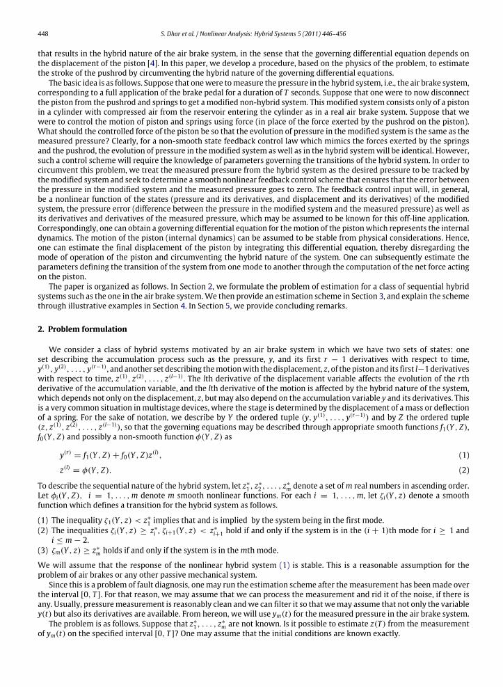
(y − Patm)Ab − C1z2 − K1z1, y < Pth,(y − Patm)Ab − C2z2 − K2z1, y ≥ Pth, z1 < zclearance,(y − Patm)Ab − C3z2 − K3z1, z1 ≥ zclearance,

ym = y (8)

450 S. Dhar et al. / Nonlinear Analysis: Hybrid Systems 5 (2011) 446–456

Table 1Nomenclature of parameters/variables used.

Parameter/Variable Description value

R Gas constant for air 287 J/kg KT Ambient temperature 293 KPb Brake chamber pressure N/m2

Po Supply pressure 7.22 × 105 N/m2

Ap Area of treadle valve opening 3.1669 × 10−5 m2

xb Pushrod stroke mPatm Atmospheric pressure 101325 N/m2

Pth Push-out pressure 1.4273 × 105 N/m2

Pct Contact pressure 2.3926 × 105 N/m2

zclearance Brake pad and brake drum clearance 0.6 mmm Mass of pushrod and diaphragm 5 kgAb Area of brake chamber diaphragm 0.0129 m2

Vo1 Initial volume of brake chamber 0.00032774 m3

K1 Spring constant for Mode I 2.1972 × 103 N/mK2 Spring constant for Mode II 4.3944 × 103 N/mK3 Spring constant for Mode III 6.5916 × 103 N/mC1 Damping coefficient for Mode I 20.96 Ns/mC2 Damping coefficient for Mode II 29.64 Ns/mC3 Damping coefficient for Mode III 36.31 Ns/m

0

2

4

Pb

(N/m

2 )

Xb

(m/s

)

Xb

(m)

6

8× 105

0 10 20

time (s)

30 40 50

0 10 20

time (s)

30 40 50

0 10 20

time (s)

30 40 50

1.5

1

0.5

0

–3

–2

–1

0

1

2

3

.

Fig. 2. Simulated response of the hybrid system.

where ym is the (measured) output of the system during [0, T ]. A typical simulated response of the pneumatic system (7)for the parameter values listed in Table 1 is shown in Fig. 2.

4.1. Estimation of the parameters of the hybrid system

We consider the following nonlinear system for the purpose of steady-state parameter estimation, by first neglectingthe mass m of the piston. As explained earlier, we then construct a modified system in which the pushrod is disconnectedfrom the piston. Since the inertia of the piston is neglected, the velocity of the piston may be thought of as a control inputwhich may be specified arbitrarily. Correspondingly, the governing equations for the hybrid and the modified system maybe expressed as

S. Dhar et al. / Nonlinear Analysis: Hybrid Systems 5 (2011) 446–456 451

y =

Apy2RT log

Poy

− Abz1y

Abz1 + Vo1,

z1 =

1C1

[(y − Patm)Ab − K1z1] , y < Pth,

1C2

[(y − Patm)Ab − K2z1] , y ≥ Pth, z1 < zclearance,

1C3

[(y − Patm)Ab − K3z1] , z1 ≥ zclearance,

ym = y. (9)

The non-hybrid system for estimation of the steady-state parameter z1(T ) of the hybrid system (9) is therefore

y =

Apy2RT log

Poy

− Abuvy

Abz1 + Vo1,

z1 = uv, (10)

where uv is the control input. We follow the procedure mentioned in Section 3, i.e., we design the controller uv for (10) suchthat y(t) exactly matches ym(t) on the interval [0, T ]. The measured output of the hybrid system (9) may be assumed to besufficiently smooth, i.e., ym, ym are available.

From (10), we can see that the control input uv affects the first time derivative of the output. If we were to set the right-hand side of the equation for y in (10) to be equal ym − k1(y− ym) for some k1 > 0, then the error e(t) := y− ym will evolveaccording to the following differential equation:

e + k1e = 0.

In other words, the error will converge to zero exponentially, and the rate of convergence is governed by k1, which maybe chosen so that the error response is fast enough for the identification to be performed in the interval [0, T ]. The controlinput uv that ensures that the right-hand side of the equation for y in (10) is equal to ym − k1(y − ym) is given by

uv =1Aby

[−(ym − k1(y − ym))(Abz1 + Vo1)+ φ(y)] , (11)

where φ(y) = Apy2RT log

Poy

, and since y is strictly positive on the interval [0, T ], Apy = 0. However, for exact tracking,

y(t) = ym(t) for t ∈ [0, T ]. Therefore, replacing ywith ym in (10) and substituting for uv from (11), we get the estimator forz1 as follows:

˙z1 =1

Abym

−ym(Abz1 + Vo1)+ φ(ym)

,

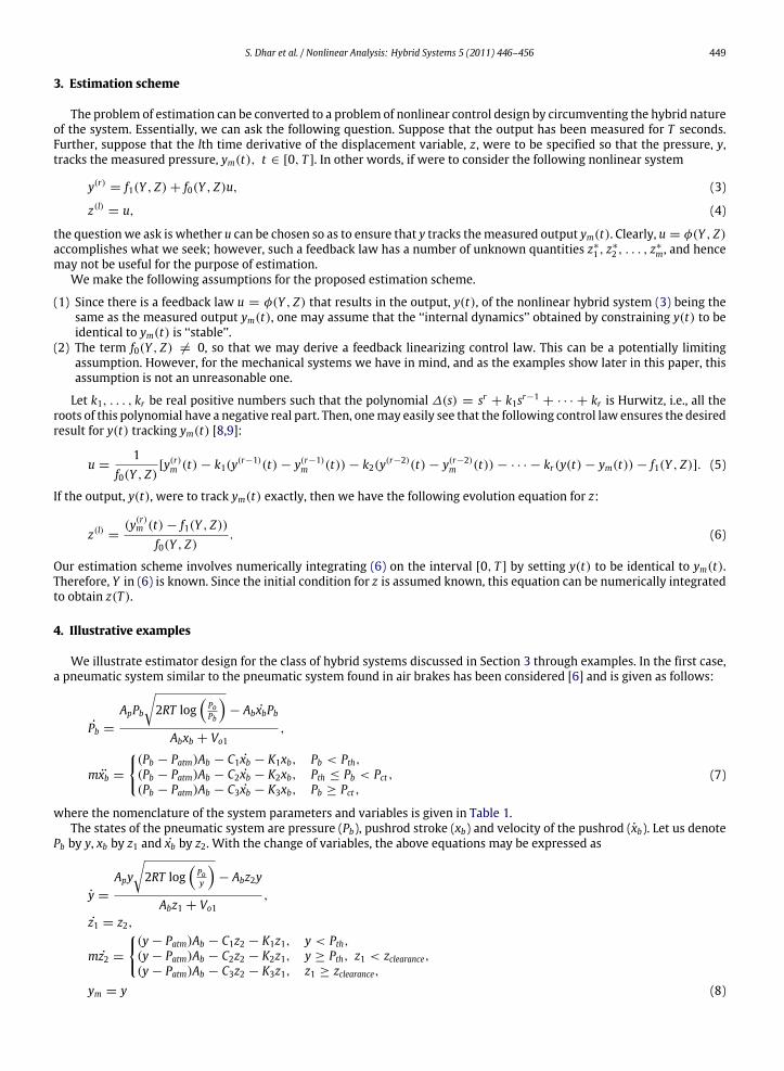
z1(0) = 0. (12)

Simulations, in Fig. 3, show that in the steady state z1 tends to z1 of the hybrid system.In cases where themassm of the piston is significant and cannot be neglected, the derivation of the control input is more

complicated. We consider such a case now:

y =

Apy2RT log

Poy

− Abz2y

Abz1 + Vo1,

z1 = z2,z2 = ua, (13)

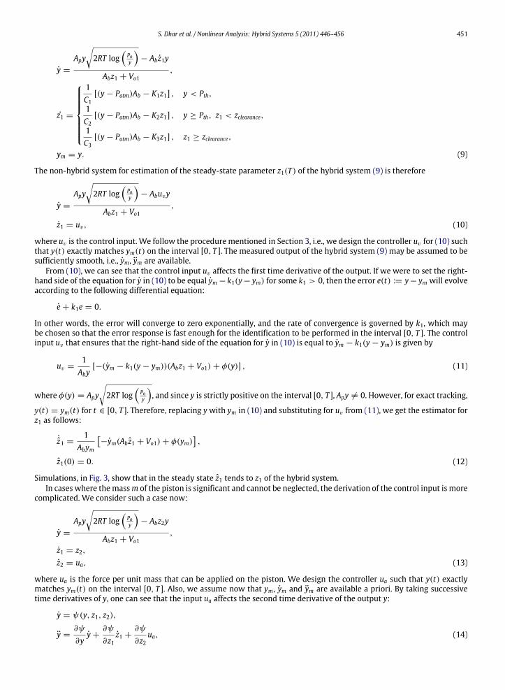
where ua is the force per unit mass that can be applied on the piston. We design the controller ua such that y(t) exactlymatches ym(t) on the interval [0, T ]. Also, we assume now that ym, ym and ym are available a priori. By taking successivetime derivatives of y, one can see that the input ua affects the second time derivative of the output y:

y = ψ(y, z1, z2),

y =∂ψ

∂yy +

∂ψ

∂z1z1 +

∂ψ

∂z2ua, (14)

452 S. Dhar et al. / Nonlinear Analysis: Hybrid Systems 5 (2011) 446–456

1.4

1.2

1

0.8

Z1

(m)

0.6

0.4

0.2

00 5 10 15 20 25 30

time (s)35 40 45 50

Z1

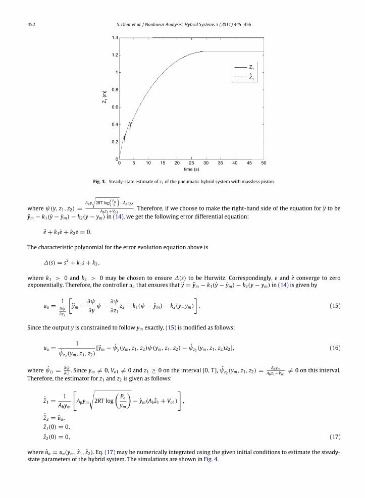
Z1

Fig. 3. Steady-state estimate of z1 of the pneumatic hybrid system with massless piston.

where ψ(y, z1, z2) =

Apy2RT log

Poy

−Abz2y

Abz1+Vo1. Therefore, if we choose to make the right-hand side of the equation for y to be

ym − k1(y − ym)− k2(y − ym) in (14), we get the following error differential equation:

e + k1e + k2e = 0.

The characteristic polynomial for the error evolution equation above is

∆(s) = s2 + k1s + k2,

where k1 > 0 and k2 > 0 may be chosen to ensure ∆(s) to be Hurwitz. Correspondingly, e and e converge to zeroexponentially. Therefore, the controller ua that ensures that y = ym − k1(y − ym)− k2(y − ym) in (14) is given by

ua =1∂ψ

∂z2

[ym −

∂ψ

∂yψ −

∂ψ

∂z1z2 − k1(ψ − ym)− k2(y−ym)

]. (15)

Since the output y is constrained to follow ym exactly, (15) is modified as follows:

ua =1

ψz2(ym, z1, z2)[ym − ψy(ym, z1, z2)ψ(ym, z1, z2)− ψz1(ym, z1, z2)z2], (16)

where ψ() =∂ψ

∂(). Since ym = 0, Vo1 = 0 and z1 ≥ 0 on the interval [0, T ], ψz2(ym, z1, z2) =

AbymAbz1+Vo1

= 0 on this interval.Therefore, the estimator for z1 and z2 is given as follows:

˙z1 =1

Abym

Apym

2RT log

Poym

− ym(Abz1 + Vo1)

,

˙z2 = ua,

z1(0) = 0,

z2(0) = 0, (17)

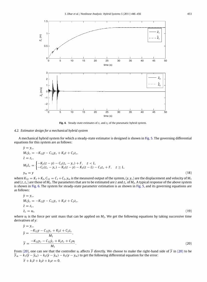
where ua = ua(ym, z1, z2). Eq. (17) may be numerically integrated using the given initial conditions to estimate the steady-state parameters of the hybrid system. The simulations are shown in Fig. 4.

S. Dhar et al. / Nonlinear Analysis: Hybrid Systems 5 (2011) 446–456 453

1.5

1

0.5

Z1

(m)

Z2

(m/s

)

00 5 10 15 20 25

time (s)

30 35 40 45 50

0 5 10 15 20 25

time (s)

30 35 40 45 50

3

2

1

0

–1

–2

–3

Z1

Z1

Z2

Z2

Fig. 4. Steady-state estimates of z1 and z2 of the pneumatic hybrid system.

4.2. Estimator design for a mechanical hybrid system

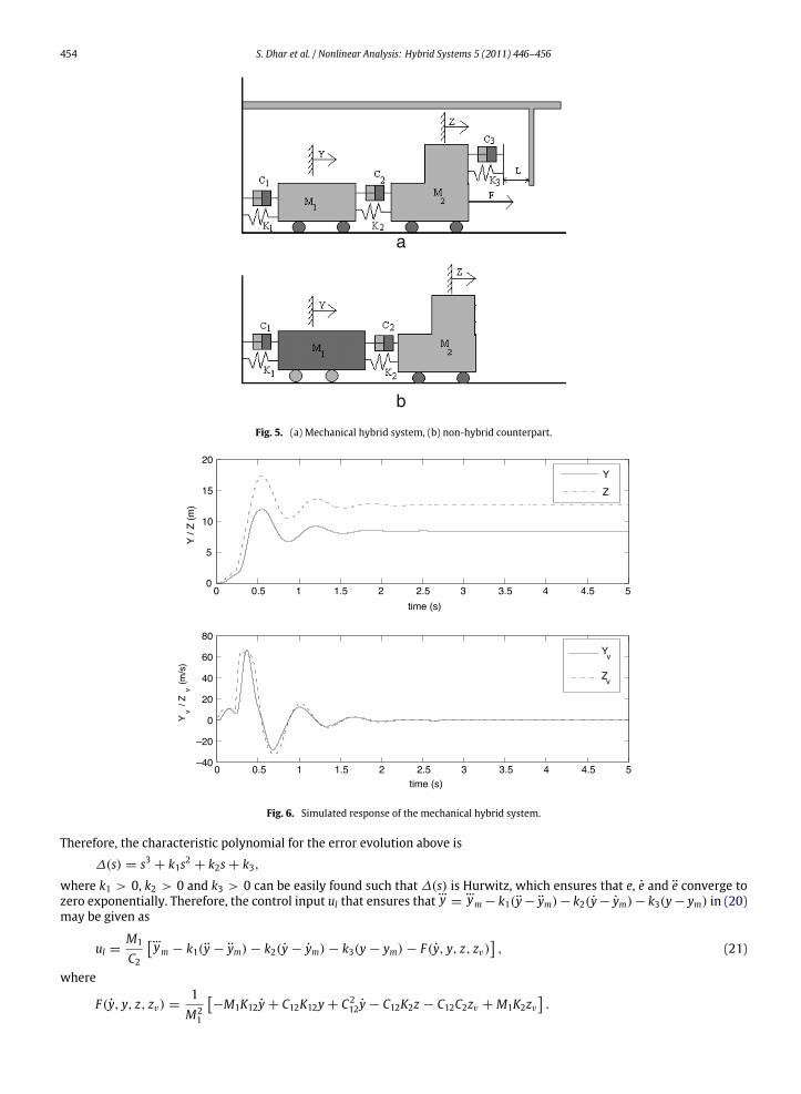
A mechanical hybrid system for which a steady-state estimator is designed is shown in Fig. 5. The governing differentialequations for this system are as follows:

y = yv,M1yv = −K12y − C12yv + K2z + C2zv,z = zv,

M2zv =

−K2(z − y)− C2(zv − yv)+ F , z < L,−C2(zv − yv)− K2(z − y)− K3(z − L)− C3zv + F , z ≥ L,

ym = y (18)

where K12 = K1 +K2, C12 = C1 +C2, ym is themeasured output of the system, (y, yv) are the displacement and velocity ofM1and (z, zv) are those ofM2. The parameters that are to be estimated are z and zv ofM2. A typical response of the above systemis shown in Fig. 6. The system for steady-state parameter estimation is as shown in Fig. 5, and its governing equations areas follows:

y = yv,M1yv = −K12y − C12yv + K2z + C2zv,z = zv,zv = ul, (19)

where ul is the force per unit mass that can be applied on M2. We get the following equations by taking successive timederivatives of y:

y = yv,

y =−K12y − C12yv + K2z + C2zv

M1,

...y =

−K12yv − C12yv + K2zv + C2ul

M1. (20)

From (20), one can see that the controller ul affects...y directly. We choose to make the right-hand side of

...y in (20) to be...

ym − k1(y − ym)− k2(y − ym)− k3(y − ym) to get the following differential equation for the error:...e + k1e + k2e + k3e = 0.

454 S. Dhar et al. / Nonlinear Analysis: Hybrid Systems 5 (2011) 446–456

a

b

Fig. 5. (a) Mechanical hybrid system, (b) non-hybrid counterpart.

0 0.5 1 1.5 2 2.5 3 3.5 4 4.5 50

5

10

15

20

time (s)

Y /

Z (

m)

0 0.5 1 1.5 2 2.5 3 3.5 4 4.5 5time (s)

Yv /

Zv (

m/s

)

Yv

Zv

Y

Z

–40

–20

0

20

40

60

80

Fig. 6. Simulated response of the mechanical hybrid system.

Therefore, the characteristic polynomial for the error evolution above is

∆(s) = s3 + k1s2 + k2s + k3,

where k1 > 0, k2 > 0 and k3 > 0 can be easily found such that ∆(s) is Hurwitz, which ensures that e, e and e converge tozero exponentially. Therefore, the control input ul that ensures that

...y =

...ym − k1(y− ym)− k2(y− ym)− k3(y− ym) in (20)

may be given as

ul =M1

C2

...ym − k1(y − ym)− k2(y − ym)− k3(y − ym)− F(y, y, z, zv)

, (21)

where

F(y, y, z, zv) =1M2

1

−M1K12y + C12K12y + C2

12y − C12K2z − C12C2zv + M1K2zv.

S. Dhar et al. / Nonlinear Analysis: Hybrid Systems 5 (2011) 446–456 455

Z (

m)

Zv

(m/s

)

time (s)

0 0.5 1 1.5 2 2.5 3 3.5 4 4.5 5

time (s)

0 0.5 1 1.5 2 2.5 3 3.5 4 4.5 5

0

5

10

15

20

80

60

40

20

0

–20

–40

Z

Z

Zv

Zv

Fig. 7. Steady-state estimates of z and zv of the mechanical hybrid system.

For exact tracking, we set y(t) to be identical to ym(t), for t ∈ [0, T ], in (21) to get ul as follows:

ul =M1

C2

...ym − F(ym, ym, z, zv)

. (22)

Therefore, the estimator for z and zv is given as follows:

˙z =1C2

[M1ym + K12ym + C12ym − K2z],

˙zv = ul,

z(0) = 0,

zv(0) = 0, (23)

where ul can be obtained by substituting z = z and zv = zv in (22). Fig. 7 portrays the estimates of z and zv that are obtainedby numerically integrating (23) for the given initial conditions.

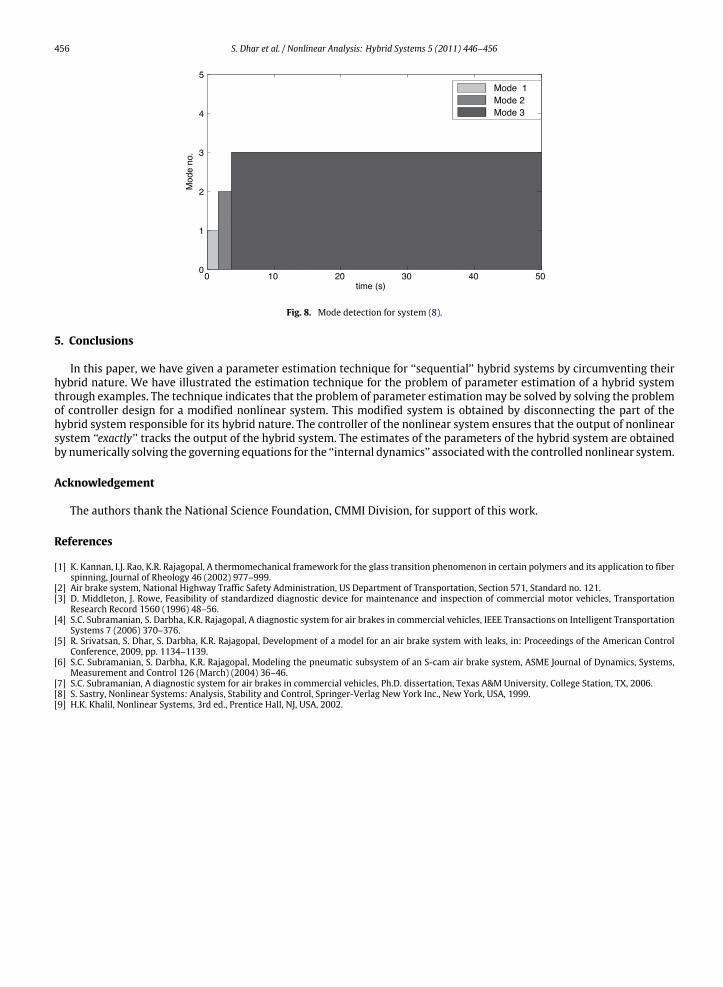
4.3. Mode detection

Weuse the estimates of states Z = (z1, z2) of the hybrid system (8) to determine themode the system is in at any instantof time t ∈ [0, T ]. The mode i (i = 1, 2, 3) and the time duration ∆i for that mode may be obtained by determining thetime instants for which |φi(Ym, Z)− u| is minimum. For the hybrid system (8), φi(Ym, Z) (i = 1, 2, 3) are given as follows:

φ1(Ym, Z) =1m

[(ym − Patm)Ab − C1z2 − K1z1],

φ2(Ym, Z) =1m

[(ym − Patm)Ab − C2z2 − K2z1],

φ3(Ym, Z) =1m

[(ym − Patm)Ab − C3z2 − K3z1],

where Z = (z1, z2) are the system’s estimated states and Ym = ym is its measured output.We define the following residualsfor each φi(Ym, Z), over the time interval [0, T ]:

ϵ1 = |φ1(Ym, Z)− u|,

ϵ2 = |φ2(Ym, Z)− u|,

ϵ3 = |φ3(Ym, Z)− u|,

where u = ua and is given by (16). Therefore, ∆i is the largest set of the continuous sequence of time instants in [0, T ] forwhich the corresponding ϵi is minimum. The system is said to be in mode i, at least, for all t ∈ ∆i. Fig. 8 shows the modessystem (8) is in over the time interval [0, T ] and the likely time duration for the system in each of these modes.

456 S. Dhar et al. / Nonlinear Analysis: Hybrid Systems 5 (2011) 446–456

0 10 20 30 40 500

1

2

3

4

5

time (s)

Mod

e no

.

Mode 1Mode 2Mode 3

Fig. 8. Mode detection for system (8).

5. Conclusions

In this paper, we have given a parameter estimation technique for ‘‘sequential’’ hybrid systems by circumventing theirhybrid nature. We have illustrated the estimation technique for the problem of parameter estimation of a hybrid systemthrough examples. The technique indicates that the problem of parameter estimationmay be solved by solving the problemof controller design for a modified nonlinear system. This modified system is obtained by disconnecting the part of thehybrid system responsible for its hybrid nature. The controller of the nonlinear system ensures that the output of nonlinearsystem ‘‘exactly’’ tracks the output of the hybrid system. The estimates of the parameters of the hybrid system are obtainedby numerically solving the governing equations for the ‘‘internal dynamics’’ associatedwith the controlled nonlinear system.

Acknowledgement

The authors thank the National Science Foundation, CMMI Division, for support of this work.

References

[1] K. Kannan, I.J. Rao, K.R. Rajagopal, A thermomechanical framework for the glass transition phenomenon in certain polymers and its application to fiberspinning, Journal of Rheology 46 (2002) 977–999.

[2] Air brake system, National Highway Traffic Safety Administration, US Department of Transportation, Section 571, Standard no. 121.[3] D. Middleton, J. Rowe, Feasibility of standardized diagnostic device for maintenance and inspection of commercial motor vehicles, Transportation

Research Record 1560 (1996) 48–56.[4] S.C. Subramanian, S. Darbha, K.R. Rajagopal, A diagnostic system for air brakes in commercial vehicles, IEEE Transactions on Intelligent Transportation

Systems 7 (2006) 370–376.[5] R. Srivatsan, S. Dhar, S. Darbha, K.R. Rajagopal, Development of a model for an air brake system with leaks, in: Proceedings of the American Control

Conference, 2009, pp. 1134–1139.[6] S.C. Subramanian, S. Darbha, K.R. Rajagopal, Modeling the pneumatic subsystem of an S-cam air brake system, ASME Journal of Dynamics, Systems,

Measurement and Control 126 (March) (2004) 36–46.[7] S.C. Subramanian, A diagnostic system for air brakes in commercial vehicles, Ph.D. dissertation, Texas A&M University, College Station, TX, 2006.[8] S. Sastry, Nonlinear Systems: Analysis, Stability and Control, Springer-Verlag New York Inc., New York, USA, 1999.[9] H.K. Khalil, Nonlinear Systems, 3rd ed., Prentice Hall, NJ, USA, 2002.