Identification of non-stationary dynamical systems using multivariateARMA models

Mathieu Bertha∗, Jean-Claude GolinvalUniversity of Liege, Department of Aerospace and Mechanical Engineering,

Allee de la Decouverte 9, 4000 Liege, Belgium

AbstractThis paper is concerned by the modal identification of time-varying mechanical systems. Based on previousworks about autoregressive moving average models in vector form (ARMAV) for the modal identificationof linear time invariant systems, and time-varying autoregressive moving average models (TV-ARMA) forthe identification of nonstationary systems, a time-varying ARMAV (TV-ARMAV) model is presented forthe multivariate identification of time-varying systems. It results in the identification of not only the time-varying poles of the system but also of its respective time-varying mode shapes. The method is applied ona time-varying structure composed of a beam on which a mass is moving.

Keywords: Time-varying systems, modal identification, vector auto-regressive moving average modeling,basis functions, moving mass problem

Introduction

In the field of structural engineering, modal analysis represents a significant part. Whether numerical orexperimental, modal analysis is a mature topic when the assumptions of linearity and time-invariance aremet for the structure to be analyzed. Nowadays, the challenges mainly focus on nonlinear modal analysisand time (or any other parameter) dependence of linear systems [1]. In both cases, the response signalsrecorded on the structure exhibit nonstationary behaviors.

The loss of the stationary assumption directly impacts the identification methods. New signal processingtools are then required to take the time variation into account. Time-frequency methods were designed forthis purpose, the simplest one being the Short-Time Fourier Transform (STFT). This method simply appliesthe traditional Fourier transform on short time windows by assuming a piecewise stationarity of the signal.By applying this kind of methods, it is obvious that there is a trade-off between the frequency resolutionand the ability to follow the variation of the signal properties. This kind of approach is also used for themodal analysis of time-varying structures by applying standard modal analysis methods on short slidingtime windows where the response signals are assumed stationary. For example, the Stochastic SubspaceIdentification (SSI) method is applied on a bridge-like structure on short time windows in [2] and in [3] avariant of this method (the Crystal Clear SSI method) is applied on flight data of the Ariane 5 launcher totrack the variation of its modal properties due to its decrease in mass with time.

Other time-frequency methods are also employed for their ability to track variations in the signals. Onecan cite the wavelet decomposition that can be used for the modal analysis of time-varying systems [2, 4, 5, 6].The tracking of instantaneous frequencies may also be performed by signal decomposition methods. TheHilbert-Huang Transform (HHT) [7] based on the Empirical Mode Decomposition (EMD) method and theHilbert Vibration Decomposition (HVD) [8] method are able to decompose multicomponent signal into its

∗Corresponding authorEmail addresses: mathieu.bertha@ulg.ac.be (Mathieu Bertha), jc.golinval@ulg.ac.be (Jean-Claude Golinval)

Preprint submitted to Elsevier November 28, 2016

monocomponent constitutive parts, which are called Intrinsic Mode Functions (IMF). These two methodsdiffer in the way they work but they are both based on the Hilbert transform and they are able to extractinstantaneous amplitude and frequency of each monocomponent. In [9], the EMD method is used for theidentification of a time-varying multiple degrees of freedom (MDOF) system and the HVD method is alsoapplied on a MDOF system in [10, 11].

Another interesting way to proceed to the identification of time-varying systems is to build a parametricmodel in which the parameters to identify are free to vary with time. Such models, if they are properlydesigned, show good performances in terms of accuracy of the identification as well as with respect to theirability to track the dynamics variability of the underlying system. Autoregressive Moving-Average (ARMA)or State-Space (SS) models are often used for that purpose. In [12, 13, 14], the identification of time-varyingsystems is performed through the identification state-space models in which the state transition matrix isfree to vary with time. An eigenvalue decomposition of this series of matrices results in what the authorcalled the pseudo-modal parameters. In [15, 16] the estimation of time-varying ARMA models is performedby the Basis Function (BF) approach. In that method, the time-varying parameters of the model areexpanded in a series of chosen time functions. This kind of models was first used in [17] for the estimationof evolutionary spectral density by a second-order Taylor series expansion of the parameters. In the fieldof structural dynamics, this method is applied in several different ARMA models (time dependent ARMA(TARMA), functional series TARMA (FS-TARMA), ...) by Fassois et al. [18, 19]. Most of the studies abouttime-varying systems deal with univariate time series and in the present paper, we use ARMA models in amultivariate form. Let us note that a similar study was performed in [20] but we focus here on the abilityto well identify the varying mode shapes of the tested structure which are an important modal property instructural engineering. The latter mode shapes are validated by comparison with an analytical model of theproblem. The identified mode shapes are then used for post identification of the position of the mass usingan error localization process between a reference set of mode shapes and the time-varying ones.

The paper is organized as follows. Section 1 presents the method for the multivariate identificationof TV systems. To illustrate the application of the method, an experimental demonstration structurewas built and is firstly presented in Section 2. The time-varying identification is then performed and theobtained results are illustrated in Section 3. For validation purposes, a simple Rayleigh-Ritz model is builtto accurately represent the dynamics of the problem and easily introduce the structural variation. It ispresented in Section 4 together with its correlation with the experimental results. In Section 5, based onthe identified mode shapes an application of localization of the variable part of the system is presented. Thelast section concludes the paper by recalling all the aspects of the work such as the difficulties that this kindof identification faces, the results we obtain and the possible applications of the identification of the modetime-varying shapes.

1. Time-varying multivariate auto-regressive moving average model

In this section, the method of Auto-Regressive Moving Average in Vector form (ARMAV) is first recalledin the field of linear time invariant (LTI) system identification. It leads to the determination of the modalproperties in terms of poles (eigen frequencies ωr and damping ratio’s ζr) as well as mode shapes vr of thestructure. Next, the method is extended to the time-varying behavior using the basis function approachas proposed in the FS-TARMA method but in a multivariate form. Accordingly, the parameters to beestimated become matrices instead of scalar coefficients.

1.1. The ARMAV method for output-only modal identificationThe ARMAV method is able to perform modal identification of a structure based only on response

measurements (output-only identification). A required assumption is that the external excitation generatingthe response of the structure is an uncorrelated white noise. This method is commonly used in the field ofstructural dynamics, see for example [21, 22, 23].

2

Let us note y[t] the d×1 multivariate responses measurement vector of the structure. The ARMAV(p, q)model of the output signal writes:

y[t] +p∑i=1

Ai y[t− i] = e[t] +q∑j=1

Bj e[t− j], (1)

where the innovation e[t] is a zero-mean uncorrelated white noise process. The p Ai matrix coefficientsrepresent the autoregressive part of the model that contains the dynamic information of the system. Theother q Bj matrix coefficients constitute the moving average part of the model.

The relationship between an ARMAV model and a mechanical system is established in [24, 21]. Let usconsider a mechanical system of order n for which the governing equation writes

M y(t) +C y(t) +K y(t) = f(t) (2)

and suppose that we measure all the n degrees of freedom. Transforming the system in its state-spacerepresentation, it may be shown that an ARMAV(2, 1) is able to describe the dynamics of the system (2).Further, it is shown in [21] that in the presence of measurement noise, an ARMAV(2, 2) should rather beused instead of ARMAV(2, 1). But this result is valid if the dimension d of the multivariate response vectormatches exactly the actual dimension n of the mechanical system. When it is not the case, ARMAV(2m,2m− 1) or ARMAV(2m, 2m) are to be used with m equal to the rounded up value of n/d.

1.2. Time-varying ARMAV modelLet us now consider the problem of time-varying mechanical systems where it is assumed that the rate of

variation of the system is slow with respect to the period of vibration (i.e. the term M(t) y(t) is negligible):

M(t) y(t) +C(t) y(t) +K(t)y(t) = f(t) (3)

Because of the time dependence of the system matrices, the dynamic behavior of the system is also time-dependent, i.e. its modal properties (eigen frequencies ωr(t),damping ratio’s ζr(t) and mode shapes vr(t))are not constant anymore.

Regarding to the signal model (1), the time dependence have to be captured by the AR and MA co-efficients. It follows that the ARMAV model in the framework of LTV systems is simply obtained bytime-dependent matrices Ai[t] and Bj [t], i.e.:

y[t] +p∑i=1

Ai[t]y[t− i] = e[t] +q∑j=1

Bj [t] e[t− j]. (4)

The coefficients to be estimated are now the time-varying Ai[t] and Bj [t] matrices. The key idea of thebasis functions approach is to project these matrices on a previously selected set of known time functionsfk[t].

Ai[t] =rA∑k=1

Ai,k fk[t] (5)

Bj [t] =rB∑k=1

Bj,k fk[t] (6)

There are many possible choices for the basis functions and the most commonly used are polynomials(Legendre, Chebyshev, ...) or trigonometric functions, as in the following. Similar results may be obtainedusing each kind of basis but sometimes requiring different sizes of the function bases. Note that if the systemexhibit a known structure in its varying properties, it could be used to provide structured basis functions to

3

the method. In this way, the identification problem becomes a time invariant problem when looking for theprojection coefficients Ai,k and Bj,k. Introducing (5) and (6) into (4) yields to

y[t] +p∑i=1

rA∑k=1

Ai,k fk[t]y[t− i] = e[t] +q∑j=1

rB∑k=1

Bj,k fk[t] e[t− j]. (7)

As previously said, the aim of the method is to identify the AR and MA projection coefficients. To doso, let us first gather all these coefficients in a single matrix Θ:

Θ = [A1,1, A1,2, · · · , A1,rA, A2,1, · · · , Ap,rA

, B1,1, · · · , Bq,rB] . (8)

In the same way, the product of the basis functions and the lagged values of the output and error termare also put in the following vector forms:

φ[t]T =[f1[t]y[t− 1]T , f2[t]y[t− 1]T , · · · , fra [t]y[t− p]T

](9)

ψ[t]T =[−f1[t]e[t− 1]T , −f2[t]e[t− 1]T , · · · , −frb

[t]e[t− q]T]

(10)

The prediction error of the model can now be expressed by subtracting the estimate of the responsey[t,Θ] from the response signal itself y[t]:

e[t,Θ] = y[t]− y[t,Θ] (11)

where the estimate of the output signal is given by

y[t,Θ] = −p∑i=1

rA∑k=1

Ai,k fk[t]y[t− i] +q∑j=1

rB∑k=1

Bj,k fk[t] e[t− j]. (12)

Using the notations (8), (9) and (10), the prediction error becomes

e[t,Θ] = y[t] + Θ[φ[t]ψ[t]

](13)

The matrix regression parameters of the system can be found by minimizing a positive scalar cost functionof the modeling error with respect to the parameters. A commonly used cost function is the Sum of SquaredErrors (SSE) defined as

V (Θ) = 1N

N∑t=1

e[t,Θ]T e[t,Θ], (14)

where N is the number of data samples. A good estimate of Θ is given by the minimum of V (Θ), i.e.

Θ = arg minΘ

1N

N∑t=1

e[t,Θ]T e[t,Θ]. (15)

The latter equation leads to a nonlinear optimization problem because ψ[t] depends on the error termwhich itself depends on the Θ parameter. To solve this problem, the Multi Stage Least Squares (MSLS)method [25] is used here. It consists in building a sequence of linear least squares problems. This methodapplied in the scope of autoregressive moving average estimation is performed in two steps. First, a high-orderautoregressive model is used to fit the data which requires only a least square estimate as the nonlinearityis located in the MA part. Once this model is known, it is used to get an estimate of the innovatione[t, Θhigh order]. In the second step, an ARMAV model is estimated by using the innovation as a knowninput. The process is then iterated by updating the output and the innovation. The drawback of the MSLSmethod compared to other nonlinear optimization scheme (such as Gauss-Newton or Levenberg-Marquardt)is that a decrease in the cost function is not ensured. The latter kind of optimization problems havegood convergence properties but often suffer of high computation costs involved in the computation of thegradient and Hessian matrix of the cost function. Further, they also require a good initial guess for themodel parameters to converge to the global optimum.

4

1.3. Computation of the modal parametersOnce the basis functions coefficients are identified using the above method, the time-varying autoregres-

sive matrix coefficients can be computed at any time instants using (5). These coefficients are representativeof the instantaneous dynamics of the system at time t as if it was fixed at this time t. In this so calledfrozen-time approach, the obtained parameters are a first approximation of those of the actual time-varyingsystem and it is shown in [26, 27] that this approximation by the frozen-time approach converges to the trueparameters as the variation rate between the system properties and its dynamics decreases.

The corresponding modal parameters at time t are obtained through the so called companion matrix ofthe autoregressive part of the model:

C =

−A1[t] I 0 · · · 0−A2[t] 0 I · · · 0

......

... . . . ...

−Ap−1[t]...

... I−Ap[t] 0 0 · · · 0

(16)

It can be shown that this matrix (or some variant of it) are related to the state-space representation ofthe model [25]. The eigenvalues µr of the companion matrix are the discrete-time poles of the system andare related to the poles of the system λr by

µr = eλr ∆t, (17)

where ∆t is the sampling time step of the recorded signals. The d first components of the correspondingeigenvectors give the mode shapes of the system.

2. Modal identification of the experimental system

2.1. Presentation of the test structureThe system to be tested in this paper consist in an aluminum beam supported at its ends on which

a mass is traveling as shown in Figure 1. It is a 2.1-meter long beam with a rectangular cross section of8 × 2 centimeters. Both ends are supported by springs and bearing elements that let the rotation free atthe supports levels. The mass is chosen to be sufficiently heavy to influence the dynamics of the system.The system is randomly excited by a shaker and its response is recorded by twelve accelerometers evenlydistributed on the beam. This kind of excitation is used to always excite all the modes in the frequencyrange of interest but also because it is a usual assumption if we want to study a system using output-onlymeasurements. The traveling mass is a 3.5-kg steel block which is not negligible with respect to the mass ofthe beam (≈ 9 kg).

Figure 1: The supported beam on which the mass is moving.

This type of system is a recurrent structure used to test methods able to study time variant systems[2, 18, 28].

5

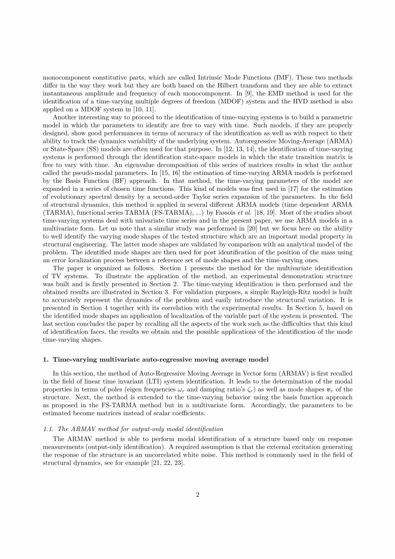
2.2. LTI modal analysis of the beam subsystemA LTI modal analysis of the beam is first performed to serve as reference. Two sensors are placed at

both ends in front of the springs and five pairs of sensors are located on each side of the beam in order tobe able to detect bending as well as torsion modes. A schematic model of the measurement setup is shownin Figure 2. For all the tests, the system is randomly excited using a shaker at coordinate 3.

Figure 2: Scheme of the excitation and recording coordinates.

Data acquisition and excitation control are carried out using the LMS Scadas Mobile system. Signal pro-cessing and modal analysis itself are performed using the PolyMAX method [29] available in LMS Test.Lab.The results of the identification are summarized in Figure 3 and Table 1.

Mode # fr [Hz] ζr [%] Type of mode1 9.86 0.32 First bending2 30.12 0.52 Opposite phase spring motion with

small second bending3 38.6 0.65 In phase spring motion with small first

bending4 53.14 0.27 Second bending5 62.17 1.56 Rotation around the beam axis6 99.70 0.28 Third bending7 168.60 0.99 Fourth bending

Table 1: Experimental modal parameters of the supported beam.

2.3. Time-Varying modal analysis of the beam-mass systemFor this test, the random excitation is turned on and the mass is pulled by hand using a simple wire

while its displacement is recorded by a laser position sensor. The acquisition time is around 50 seconds butonly the part when the mass is moving from the left to the right end is kept. The total amount of data isa record of 42 second sampled at 400 Hz for each channel. The output of the laser sensor corresponds to alinearly increasing voltage from 0 V (when the mass is located at the left end of the beam) to 10 V (whenthe mass reaches the right end). For illustration, Figure 4 shows the displacement of the mass with respectto time during the experiment. This motion has a strong influence on the dynamics of the system. Whenthe mass travels along the beam, it locally increases the inertia force at its instantaneous position.

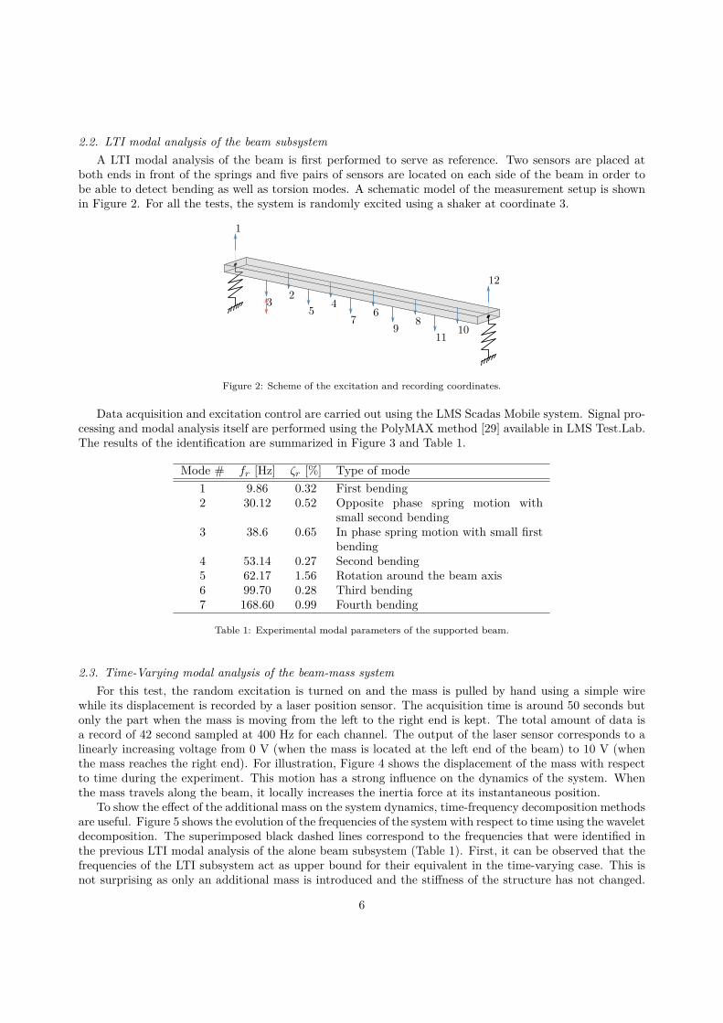
To show the effect of the additional mass on the system dynamics, time-frequency decomposition methodsare useful. Figure 5 shows the evolution of the frequencies of the system with respect to time using the waveletdecomposition. The superimposed black dashed lines correspond to the frequencies that were identified inthe previous LTI modal analysis of the alone beam subsystem (Table 1). First, it can be observed that thefrequencies of the LTI subsystem act as upper bound for their equivalent in the time-varying case. This isnot surprising as only an additional mass is introduced and the stiffness of the structure has not changed.

6

2000 10050 15010 20 30 40 60 70 80 90 110 120 130 140 160 170 180

Frequency [Hz]

CM

IF

s s s ss s s vv s s s vs s s ss v s sv s s s vs s s vv o s sv s s s vv s s vv o s vv s s s vs s s ss s s vv s s sv s s vv s s sv s s s os s s ss s s vv s s s vs s s ss s s vv s s s vs s s ss ss sv s s s vs s s ss ss sv s s s vv s s ss os sv s s s vv o s s vs os vv s s s vv v s s ss ss vv s s s vs v s s ss ss sv s s s vs v s s ss ss sv s s s vv v s s ss vs vv s s s ss v s s ss sv vv s s s vo s v s s ss ss sv s s s vv s v s s ss ss sv s s s vv s v s s ss ss sv s s s vv s s s ss ss sv s s s vv s s s ss ss sv s s s vv s s s ss sv sv s s s vv s o s s ss ss sv s s s vv s v s s ss ss vv s s s vv s v s s ss sv sv s s s vv s v s s ss ss sv s s s vv s v s s ss ss vv s s s v

33343536373839404142434445464748495051525354555657585960

190

εf : 1%, εζ : 1%, εV : 1%

Figure 3: Stabilization diagram of the beam subsystem. The selected poles are appear as bold black s.

0 5 10 15 20 25 30 35 40 45 500

5

10

Time [s]

Voltage [V]

Figure 4: Displacement of the mass with respect to time. The dashed lines represent the selected portion of the data used inthe following identification.

The instantaneous frequencies of the bending modes show a series of minima and maxima. It is easy tounderstand in this example that the maximum frequency drops occur when the mass is located at antinodesof vibration because the added inertia forces are maximum at these positions. Conversely, when the massis located at a node of vibration of a specific mode, the participation of the mass to the response of thatmode completely disappears and the frequency of the mode comes back to its initial value. Finally, theperturbation of the mass on the rotation vibration mode (initially at 62.17 Hz) is more simple. Indeed, itjust corresponds to a decrease in frequency with no great dependence with respect to the position of themass. In this particular example, it happens that the frequency of the rotation mode becomes very closeto the frequency of the fourth mode of vibration initially at 53.14 Hz. Further, because the latter mode isa bending mode, it is more influenced by the position of the mass than the rotation mode. It appears nowthat these two modes show some crossings between their frequencies, what could make the identificationdifficult.

7

Figure 5: Wavelet decomposition of the response of sensor 3. The black dashed lines represent the natural frequencies of thesystem without the moving mass.

The time-varying identification method described earlier is now applied to identify the time-varying ARand MA matrices (5) and (6). The first step is to select the model to be applied to the data. The parametersto tune are the AR order, p, the MA order, q, the type of basis functions and their number (rA and rB ,for the AR and MA parts, respectively). The model orders and the number of basis functions should besufficient to properly fit the data but, according to the principle of parsimony, one should not introduceextra-parameters in the model if not necessary for the identification [30]. This also has an impact on thechoice of the basis functions. Some bases may be more suitable than others depending on the system,especially if it has an a priori known behavior (such as periodically varying system for example). A smartchoice of the type of the basis may require less functions for a similar fitting accuracy, which means lesscoefficients to identify. Usually in traditional modal analysis, a large number of models with increasingorders are used to identify a dynamic system and the results are plotted in a stabilization diagram such asthe one shown in Figure 3. The selection of the poles is then performed manually or automatically usingspecific algorithms (e.g. clustering approach). A direct extension of the concept of stabilization diagram tothe time-varying analysis would not be convenient because of the additional time dimension.

Several indicators exist to measure the fitting quality of the model taking its complexity into account.For example, one can cite among others the Akaike Final Prediction Error (FPE) or the Akaike InformationCriterion (AIC) [22, 25]. These two criteria are given by

FPE = V (Θ)1 + δ

N

1− δN

, (18)

AIC = N log [V (Θ)] + 2 δ, (19)

where δ is the number of parameters to be estimated and N the number of time samples. In our case, thenumber of parameters δ is the number of all the coefficients in all the projection matrices in (8) so that

δ = d2 p rA + d2 q rB , (20)

where d is the dimension of the output response vector y[t].Once the model orders are fixed, the difficulty is to deal with the number of calculated poles and mode

shapes. Indeed, the vector ARMA model leads to a number of poles increasing linearly with both the modelorder p of the AR part and the number of measurement degrees of freedom d (the dimension of the companion

8

matrix (16) is p d× p d). The dimension of the companion matrix may grow rapidly and exceed the actualnumber of modes in the frequency range of interest. Because of that, a huge number of spurious polesare calculated besides the physical ones. A discrimination should then be performed in order to get clearresults. In classical modal analysis this is done using the stabilization diagram. For time-varying systems,the idea followed here retain a number M of modes that looks the more physical among all the modes. In[31] the subset selection containing physical modes is done based on the radial distribution of the poles inthe complex plane and only the M poles closest to the unit circle are retained at any time step. This kind ofdiscrimination is based on the fact that the physical modes are lightly damped with respect to the spuriousones. This method can be easily implemented here but in our case we also have another information thatcan be exploited: the mode shapes. The mode shapes may also serve for discrimination purposes betweenphysical and spurious modes. Indeed, the physical modes of a real mechanical structure usually appear wellaligned in the complex plane conversely to the spurious ones that exhibit a large dispersion. One way toquantify the aligned or scattered behavior of a mode is to compute its mean phase (MP) and mean phasedeviation (MPD) which can be seen as the variance of the phase from the mean phase. Obviously, theideal value of the MPD for a physical mode is close to 0◦. In the Identification process, we will then retainonly the M modes with the lowest time-averaged MPD. Note that if we do not know the actual numberof physical modes, an automatic clustering process could be applied to distinguish the modes with a MPDclose to zero from the others. In Figure 6, an example of a physical mode 6(a) and a spurious mode 6(b)are shown. The mean phase for each mode is drawn together with their mean phase deviation. It is clearlyvisible that the spurious modes exhibit large MPD with respect to physical ones.

0.2

0.3

0.4

30

210

60

240

90

270

120

300

150

330

180 0

0.1

(a) Physical mode (low MPD)

30

210

60

240

90

270

120

300

150

330

180 0

0.10.20.30.40.5

(b) Spurious mode (high MPD)

Figure 6: Illustration of the mode phase dispersion in the complex plane for the mode shapes at t = 15s. (a) is a physicalmode at 28.65 Hz and (b) is classified as a spurious one at 185.14 Hz.

3. Results of the identification

As stated above, in order to estimate the seven modes observed previously in the stationary analysis, theautoregressive order p should be 2. Indeed 7 modes are to be identified in the frequency band and 12 sensorsare used. Using p = 2, 12 complex conjugated pairs of modes may be identified in which we would expectto be able to identify 7 physical and 5 spurious modes. The order being fixed, it remains now to select thesize of the two function bases. To do so, a set of simulation were launched with p = 2 and q = 2 and varyingsizes of the two sets of functions corresponding to the AR and MA parts. For this analysis, a Fourier basisis chosen which is composed of a unit function and a set of pairs of sine and cosine functions. The sizes ofthe two bases of functions are selected using the FPE and AIC criteria. The set of model parameters thatminimize those two criteria in the case p = q = 2 are rA = 9 and rB = 3 basis functions for the AR andMA parts, respectively. Even if the latter couple of sizes for the functions bases gives the minimum values

9

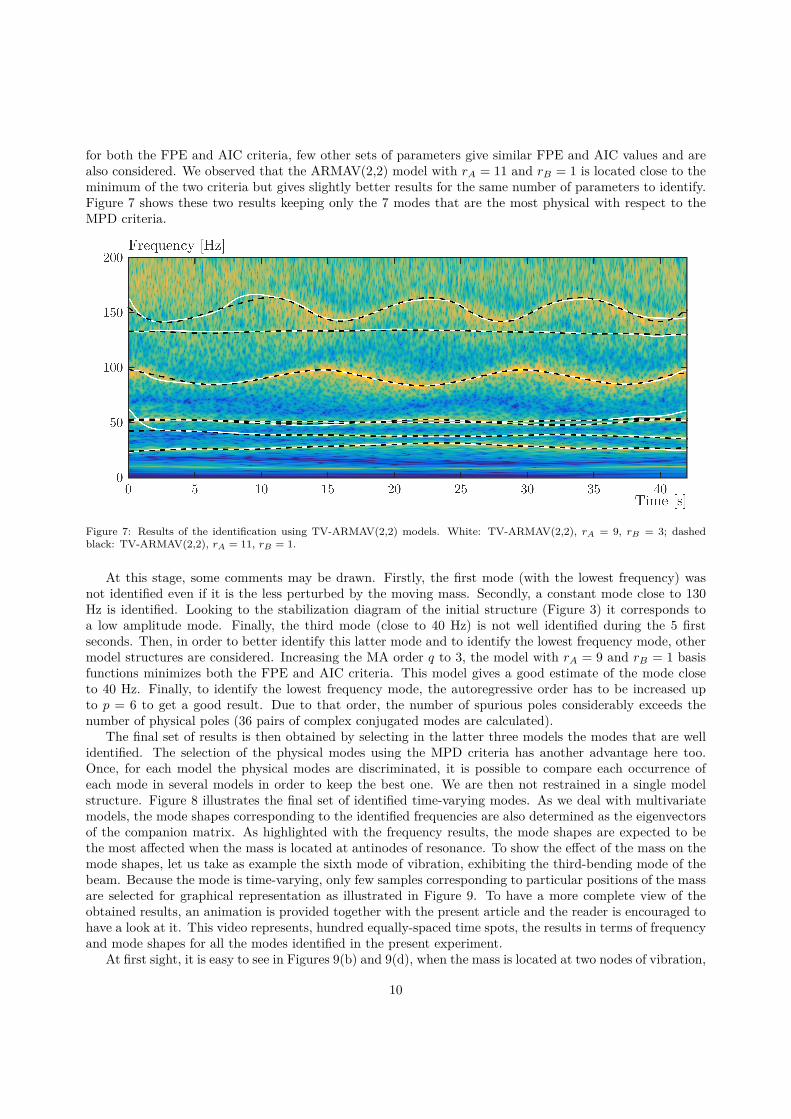
for both the FPE and AIC criteria, few other sets of parameters give similar FPE and AIC values and arealso considered. We observed that the ARMAV(2,2) model with rA = 11 and rB = 1 is located close to theminimum of the two criteria but gives slightly better results for the same number of parameters to identify.Figure 7 shows these two results keeping only the 7 modes that are the most physical with respect to theMPD criteria.

Figure 7: Results of the identification using TV-ARMAV(2,2) models. White: TV-ARMAV(2,2), rA = 9, rB = 3; dashedblack: TV-ARMAV(2,2), rA = 11, rB = 1.

At this stage, some comments may be drawn. Firstly, the first mode (with the lowest frequency) wasnot identified even if it is the less perturbed by the moving mass. Secondly, a constant mode close to 130Hz is identified. Looking to the stabilization diagram of the initial structure (Figure 3) it corresponds toa low amplitude mode. Finally, the third mode (close to 40 Hz) is not well identified during the 5 firstseconds. Then, in order to better identify this latter mode and to identify the lowest frequency mode, othermodel structures are considered. Increasing the MA order q to 3, the model with rA = 9 and rB = 1 basisfunctions minimizes both the FPE and AIC criteria. This model gives a good estimate of the mode closeto 40 Hz. Finally, to identify the lowest frequency mode, the autoregressive order has to be increased upto p = 6 to get a good result. Due to that order, the number of spurious poles considerably exceeds thenumber of physical poles (36 pairs of complex conjugated modes are calculated).

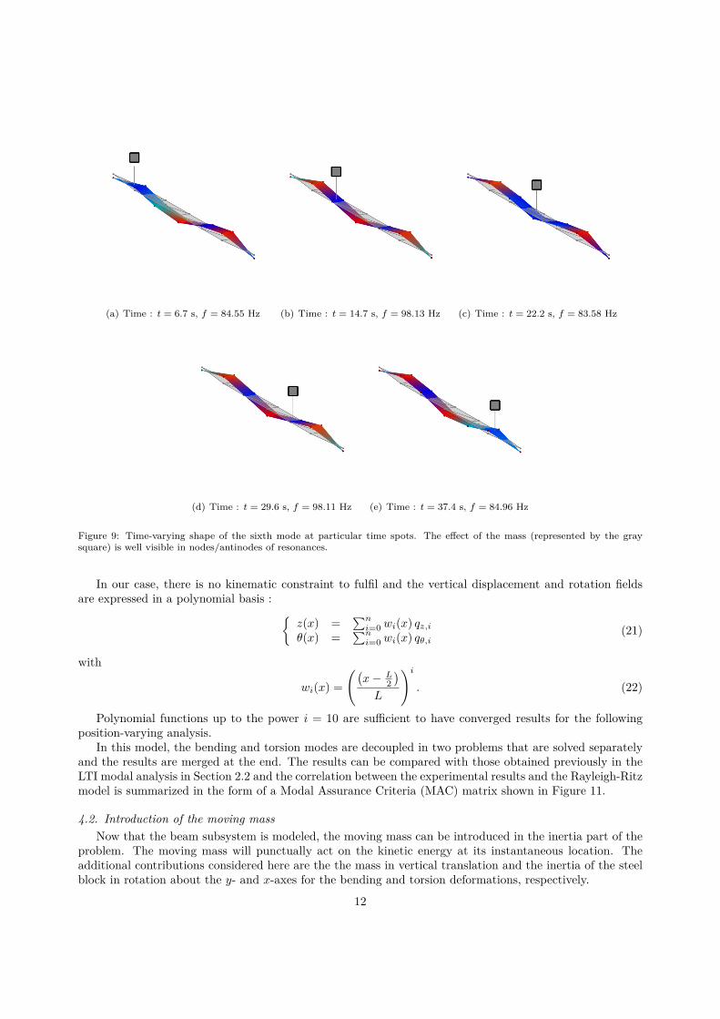
The final set of results is then obtained by selecting in the latter three models the modes that are wellidentified. The selection of the physical modes using the MPD criteria has another advantage here too.Once, for each model the physical modes are discriminated, it is possible to compare each occurrence ofeach mode in several models in order to keep the best one. We are then not restrained in a single modelstructure. Figure 8 illustrates the final set of identified time-varying modes. As we deal with multivariatemodels, the mode shapes corresponding to the identified frequencies are also determined as the eigenvectorsof the companion matrix. As highlighted with the frequency results, the mode shapes are expected to bethe most affected when the mass is located at antinodes of resonance. To show the effect of the mass on themode shapes, let us take as example the sixth mode of vibration, exhibiting the third-bending mode of thebeam. Because the mode is time-varying, only few samples corresponding to particular positions of the massare selected for graphical representation as illustrated in Figure 9. To have a more complete view of theobtained results, an animation is provided together with the present article and the reader is encouraged tohave a look at it. This video represents, hundred equally-spaced time spots, the results in terms of frequencyand mode shapes for all the modes identified in the present experiment.

At first sight, it is easy to see in Figures 9(b) and 9(d), when the mass is located at two nodes of vibration,

10

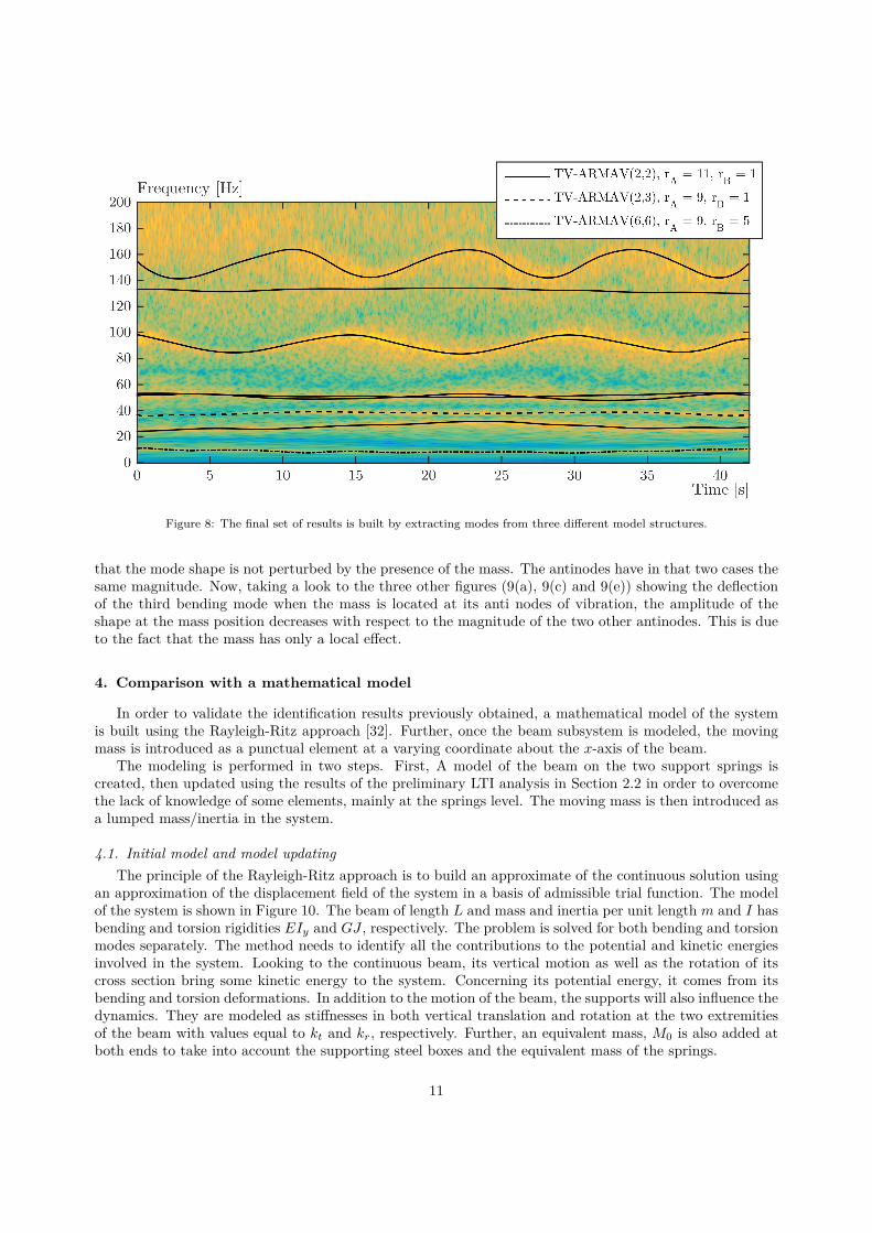
Figure 8: The final set of results is built by extracting modes from three different model structures.

that the mode shape is not perturbed by the presence of the mass. The antinodes have in that two cases thesame magnitude. Now, taking a look to the three other figures (9(a), 9(c) and 9(e)) showing the deflectionof the third bending mode when the mass is located at its anti nodes of vibration, the amplitude of theshape at the mass position decreases with respect to the magnitude of the two other antinodes. This is dueto the fact that the mass has only a local effect.

4. Comparison with a mathematical model

In order to validate the identification results previously obtained, a mathematical model of the systemis built using the Rayleigh-Ritz approach [32]. Further, once the beam subsystem is modeled, the movingmass is introduced as a punctual element at a varying coordinate about the x-axis of the beam.

The modeling is performed in two steps. First, A model of the beam on the two support springs iscreated, then updated using the results of the preliminary LTI analysis in Section 2.2 in order to overcomethe lack of knowledge of some elements, mainly at the springs level. The moving mass is then introduced asa lumped mass/inertia in the system.

4.1. Initial model and model updatingThe principle of the Rayleigh-Ritz approach is to build an approximate of the continuous solution using

an approximation of the displacement field of the system in a basis of admissible trial function. The modelof the system is shown in Figure 10. The beam of length L and mass and inertia per unit length m and I hasbending and torsion rigidities EIy and GJ , respectively. The problem is solved for both bending and torsionmodes separately. The method needs to identify all the contributions to the potential and kinetic energiesinvolved in the system. Looking to the continuous beam, its vertical motion as well as the rotation of itscross section bring some kinetic energy to the system. Concerning its potential energy, it comes from itsbending and torsion deformations. In addition to the motion of the beam, the supports will also influence thedynamics. They are modeled as stiffnesses in both vertical translation and rotation at the two extremitiesof the beam with values equal to kt and kr, respectively. Further, an equivalent mass, M0 is also added atboth ends to take into account the supporting steel boxes and the equivalent mass of the springs.

11

(a) Time : t = 6.7 s, f = 84.55 Hz (b) Time : t = 14.7 s, f = 98.13 Hz (c) Time : t = 22.2 s, f = 83.58 Hz

(d) Time : t = 29.6 s, f = 98.11 Hz (e) Time : t = 37.4 s, f = 84.96 Hz

Figure 9: Time-varying shape of the sixth mode at particular time spots. The effect of the mass (represented by the graysquare) is well visible in nodes/antinodes of resonances.

In our case, there is no kinematic constraint to fulfil and the vertical displacement and rotation fieldsare expressed in a polynomial basis : {

z(x) =∑ni=0 wi(x) qz,i

θ(x) =∑ni=0 wi(x) qθ,i

(21)

with

wi(x) =((

x− L2)

L

)i. (22)

Polynomial functions up to the power i = 10 are sufficient to have converged results for the followingposition-varying analysis.

In this model, the bending and torsion modes are decoupled in two problems that are solved separatelyand the results are merged at the end. The results can be compared with those obtained previously in theLTI modal analysis in Section 2.2 and the correlation between the experimental results and the Rayleigh-Ritzmodel is summarized in the form of a Modal Assurance Criteria (MAC) matrix shown in Figure 11.

4.2. Introduction of the moving massNow that the beam subsystem is modeled, the moving mass can be introduced in the inertia part of the

problem. The moving mass will punctually act on the kinetic energy at its instantaneous location. Theadditional contributions considered here are the the mass in vertical translation and the inertia of the steelblock in rotation about the y- and x-axes for the bending and torsion deformations, respectively.

12

Figure 10: Model of the beam for the Rayleigh-Ritz approach.

1.00

1.00

1.00

0.99

0.99

1.00

1.00

0.34

0.37

0.10

0.10

PolyMax [Hz]

9.86 30.12 38.60 53.14 62.17 99.70 168.60

Ray

leig

h-R

itz

[Hz]

9.68

30.17

38.93

52.78

62.17

98.69

168.89

0

0.2

0.4

0.6

0.8

1

Figure 11: Correlation matrix between the mathematical model of the LTI subsystem.

To compare the results from the Rayleigh-Ritz model with those of the time-varying identification, 50equally spaced time steps are selected in the time span under study and the related position of the mass forthese time steps are interpolated from the recorded location data in Figure 4.

The solution from the mathematical model in its 50 samples is plotted in Figure 12 together with thetime-varying identification. Two remarks can be drawn from that plot. First, the mathematical modelobtained by simply introducing the moving mass in the initial updated model matches globally well theidentified results. The largest discrepancies between the two sets of results lie at the beginning and at theend of the last time-varying mode. Note that the divergence at the end is related to the fast change in thelocation data close to 40 seconds.

Finally, having compared the frequencies, the mode shapes can be analyzed too. Traditionally, themode shape correlation is presented in a 2D MAC matrix representing the correlation between the modesof one set with all the other modes of the other set. Here, because the modes are no more constant, thetraditional layout of the MAC matrix is modified to integrate the time dimension. For each time instantof the Rayleigh-Ritz model, the MAC matrix coefficients are calculated then stacked in a column form. Allthe instantaneous correlations are then put one after each other to create a time-varying MAC matrix asshown in Figure 13. This kind of plot may be not optimal because it rapidly becomes cumbersome as thenumber of modes increases, it has the advantage to make the correlation lines visible. For most of the modes,the correlation between the Rayleigh-Ritz model and the experimental results are pretty good all along thetime line. Only the fifth experimental mode is concerned by a weaker correlation with its mathematicalcounterpart. The reason lies in the fact that experimental modes 4 and 5 are very close and cross themselvesseveral times during the recording process. The third mode is also concerned by a lack of correlation butonly during the first second.

13

Time [s]0 5 10 15 20 25 30 35 40

Frequency [Hz]

0

50

100

150

200 Time-varying identification

Rayleigh-Ritz model

Figure 12: Comparison of the time-varying identification and the Rayleigh-Ritz model.

5. Use of the instantaneous mode shapes to track the variation

The instantaneous mode shapes of the system may be used to track structural changes. To this end,tools initially developed for damage localization can be used. Model updating methods can be used to detectand locate errors or damages between numerical and experimental data [33] but they usually require theknowledge of the structural matrices obtained from a finite element model of the structure. In this paper, wechoose to use the Coordinate Modal Assurance Criterion (COMAC) [34] or its enhanced version (eCOMAC)[35] which are tools able to correlate the coordinates between two sets of modes. In the following, we comparethe set of experimental data of the time invariant system (beam and supports only) presented in Section 2.2and the results of the corresponding Rayleigh-Ritz model presented in Section 4.1.

The eCOMAC criterion is a vector containing as many coefficients as the number of degrees-of-freedomcontained in the mode shapes. It is computed as follows:

eCOMAC(i) =∑Nm

j=1 |Xj(i)−Zj(i)|2Nm

(23)

in which X and Z are two matrices containing two sets of corresponding mode shapes (for example fromnumerical and experimental analyses) and Nm is the number of modes used for the correlation. Let us notethat for the eCOMAC criterion, the two sets of modes have to be unit-normalized and the modes in eachpair have to be in phase.

5.1. Mass tracking using only experimental resultsHaving performed a linear time invariant modal analysis of the system before the introduction of the

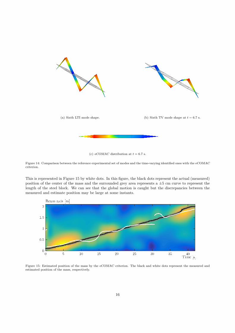
moving mass, its results can be used as a reference for the tracking of the structural modification due tothe presence of the mass. In Figure 14 the sixth mode of the beam in its nonperturbed condition (Figure14(a)), the same mode in the system containing the moving mass identified at t = 6.7 s, (Figure 14(b)) suchas in Figure 9(a) and the eCOMAC values distributed on the experimental mesh are reported. The sixthmode is used here because of the visual effect of the mass for that mode at that particular time instant butall the modes are obviously retained for the criterion calculation.

The eCOMAC criterion is calculated for each time step. Because of the rather rough experimental mesh,a cubic interpolation of the criterion is used between successive nodes along the beam to increase the spatialresolution. The position of its maximum value gives us our approximate identified position of the mass.

14

Experimental | Rayleigh-Ritz mode shapes

Time [s]

0 5 10 15 20 25 30 35 40

MA

C v

alu

e

1 | 11 | 21 | 31 | 41 | 51 | 61 | 72 | 12 | 22 | 32 | 42 | 52 | 62 | 73 | 13 | 23 | 33 | 43 | 53 | 63 | 74 | 14 | 24 | 34 | 44 | 54 | 64 | 75 | 15 | 25 | 35 | 45 | 55 | 65 | 76 | 16 | 26 | 36 | 46 | 56 | 66 | 77 | 17 | 27 | 37 | 47 | 57 | 67 | 78 | 18 | 28 | 38 | 48 | 58 | 68 | 7

0

0.1

0.2

0.3

0.4

0.5

0.6

0.7

0.8

0.9

1

Figure 13: Time-varying mode shape correlation.

15

(a) Sixth LTI mode shape. (b) Sixth TV mode shape at t = 6.7 s.

(c) eCOMAC distribution at t = 6.7 s.

Figure 14: Comparison between the reference experimental set of modes and the time-varying identified ones with the eCOMACcriterion.

This is represented in Figure 15 by white dots. In this figure, the black dots represent the actual (measured)position of the center of the mass and the surrounded grey area represents a ±5 cm curve to represent thelength of the steel block. We can see that the global motion is caught but the discrepancies between themeasured and estimate position may be large at some instants.

Figure 15: Estimated position of the mass by the eCOMAC criterion. The black and white dots represent the measured andestimated position of the mass, respectively.

16

5.2. Mass tracking using experimental results and the first mathematical modelA second approach to track the modification of the system with time is to use our first Rayleigh-Ritz

model. As shown previously in Section 4.1, this model well represents the structure. The advantage of theresults from that model instead of the results of the LTI modal analysis is that the model is a continuousapproximation of the mode shapes. It follows that we can spatially discretize it at any coordinate about thebeam axis and then refined results may be obtained far easily. The problem is then how to compare our roughmeasurement mesh with the refined numerical one. To do so, we use here expansion methods to expand ourmeasurements results to the refined numerical mesh. The System Equivalent Reduction Expansion Process(SEREP) [36] method is used to expand our results. The aim of the method is to use a set of analyticalmodes to expand the experimental ones. First, let us separate the analytical degrees-of-freedom into twosubsets, the m masters corresponding to the measured DoFs, and the s slaves DoFs. If Z represents the setof experimental mode shapes and

X =[Xm

Xs

], (24)

the (smoothed) expanded set of experimental modes is given by

Zexpanded =[ZmZs

]=[Xm TXs T

], (25)

in which the transformation matrix T is computed with the experimental modes and the pseudoinverse (†)of the analytical modes at the master nodes:

T = X†mZ. (26)

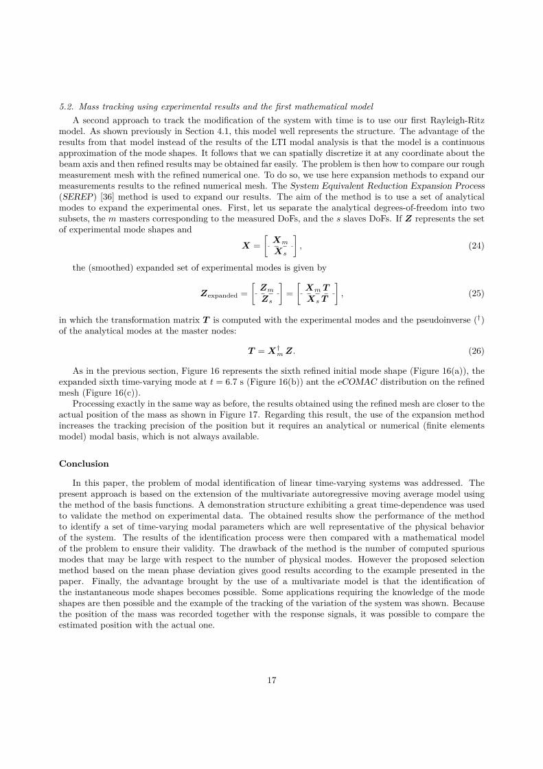
As in the previous section, Figure 16 represents the sixth refined initial mode shape (Figure 16(a)), theexpanded sixth time-varying mode at t = 6.7 s (Figure 16(b)) ant the eCOMAC distribution on the refinedmesh (Figure 16(c)).

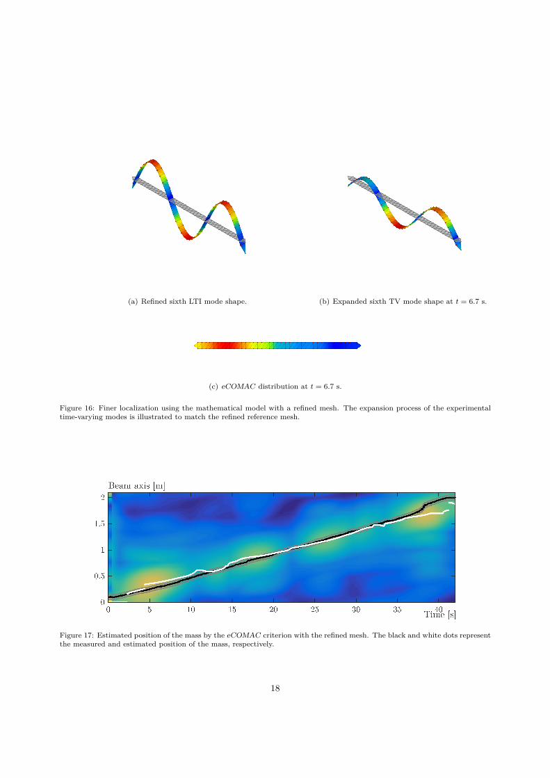
Processing exactly in the same way as before, the results obtained using the refined mesh are closer to theactual position of the mass as shown in Figure 17. Regarding this result, the use of the expansion methodincreases the tracking precision of the position but it requires an analytical or numerical (finite elementsmodel) modal basis, which is not always available.

Conclusion

In this paper, the problem of modal identification of linear time-varying systems was addressed. Thepresent approach is based on the extension of the multivariate autoregressive moving average model usingthe method of the basis functions. A demonstration structure exhibiting a great time-dependence was usedto validate the method on experimental data. The obtained results show the performance of the methodto identify a set of time-varying modal parameters which are well representative of the physical behaviorof the system. The results of the identification process were then compared with a mathematical modelof the problem to ensure their validity. The drawback of the method is the number of computed spuriousmodes that may be large with respect to the number of physical modes. However the proposed selectionmethod based on the mean phase deviation gives good results according to the example presented in thepaper. Finally, the advantage brought by the use of a multivariate model is that the identification ofthe instantaneous mode shapes becomes possible. Some applications requiring the knowledge of the modeshapes are then possible and the example of the tracking of the variation of the system was shown. Becausethe position of the mass was recorded together with the response signals, it was possible to compare theestimated position with the actual one.

17

(a) Refined sixth LTI mode shape. (b) Expanded sixth TV mode shape at t = 6.7 s.

(c) eCOMAC distribution at t = 6.7 s.

Figure 16: Finer localization using the mathematical model with a refined mesh. The expansion process of the experimentaltime-varying modes is illustrated to match the refined reference mesh.

Figure 17: Estimated position of the mass by the eCOMAC criterion with the refined mesh. The black and white dots representthe measured and estimated position of the mass, respectively.

18

References

[1] L. Garibaldi, S. Fassois, MSSP special issue on the identification of time varying structures and systems, MechanicalSystems and Signal Processing 47 (1-2) (2014) 1–2.

[2] S. Marchesiello, S. Bedaoui, L. Garibaldi, P. Argoul, Time-dependent identification of a bridge-like structure with crossingloads, Mechanical Systems and Signal Processing 23 (6) (2009) 2019–2028.

[3] M. Goursat, M. Dohler, L. Mevel, P. Andersen, Crystal Clear SSI for Operational Modal Analysis of Aerospace Vehicles,in: Proceedings of the IMAC-XXVIII, 2010, pp. 1421–1430.

[4] B. Basu, S. Nagarajaiah, A. Chakraborty, Online Identification of Linear Time-varying Stiffness of Structural Systems byWavelet Analysis, Structural Health Monitoring 7 (2008) 21–36.

[5] X. Xu, Z. Shi, Q. You, Identification of linear time-varying systems using a wavelet-based state-space method, MechanicalSystems and Signal Processing 26 (2012) 91–103.

[6] W. J. Staszewski, D. M. Wallace, Wavelet-based Frequency Response Function for time-variant systems - An exploratorystudy, Mechanical Systems and Signal Processing 47 (1-2) (2014) 35–49.

[7] N. E. Huang, S. S. Shen, Hilbert-Huang Transform and its Applications, Vol. 5 of Interdisciplinary Mathematical Sciences,World Scientific Publishing Co. Pte. Ltd., 2005.

[8] M. Feldman, Hilbert Transform Applications in Mechanical Vibration, John Wiley & Sons, Ltd, Chichester, UK, 2011.[9] Z. Shi, S. Law, X. Xu, Identification of linear time-varying MDOF dynamic systems from forced excitation using Hilbert

transform and EMD method, Journal of Sound and Vibration 321 (3-5) (2009) 572–589.[10] M. Bertha, J.-C. Golinval, Experimental modal analysis of a beam travelled by a moving mass using Hilbert Vibration

Decomposition, in: Proceedings of Eurodyn IX, Porto, 2014.[11] M. Bertha, J.-C. Golinval, Modal identification of time-varying systems using Hilbert transform and signal decomposition,

in: Proceedings of the International Conference on Noise and Vibration Engineering, ISMA 2014, Leuven, 2014, pp.2409–2419.

[12] K. Liu, Identification of Linear Time-Varying Systems, Journal of Sound and Vibration 206 (4) (1997) 487–505.[13] K. Liu, Extension of modal analysis to linear time-varying systems, Journal of Sound and Vibration 226 (1) (1999) 149–167.[14] K. Liu, L. Deng, Identification of pseudo-natural frequencies of an axially moving cantilever beam using a subspace-based

algorithm, Mechanical Systems and Signal Processing 20 (1) (2006) 94–113.[15] Y. Grenier, Time-dependent ARMA modeling of nonstationary signals, IEEE Transactions on Acoustics, Speech, and

Signal Processing 31 (4) (1983) 899–911.[16] Y. Grenier, Modeles ARMA a coefficients dependant du temps estimateurs et applications, Traitement du signal 3 (1986)

219–233.[17] T. S. Rao, The Fitting of Non-stationary Time-Series Models with Time-Dependent Parameters, Journal of the Royal

Statistical Society. Series B (Statistical Methodology) 32 (2) (1970) 312–322.[18] M. Spiridonakos, A. Poulimenos, S. Fassois, Output-only identification and dynamic analysis of time-varying mechanical

structures under random excitation: A comparative assessment of parametric methods, Journal of Sound and Vibration329 (7) (2010) 768–785.

[19] M. Spiridonakos, S. Fassois, Non-stationary random vibration modelling and analysis via functional series time-dependentARMA (FS-TARMA) models - A critical survey, Mechanical Systems and Signal Processing 47 (1-2) (2013) 1–50.

[20] M. D. Spiridonakos, S. D. Fassois, Parametric identification of a time-varying structure based on vector vibration responsemeasurements, Mechanical Systems and Signal Processing 23 (6) (2009) 2029–2048.

[21] P. Andersen, Identification of civil engineering structures using vector ARMA models, Ph.D. thesis (1997).[22] J.-B. Bodeux, J.-C. Golinval, Application of ARMAV models to the identification and damage detection of mechanical

and civil engineering structures, Smart Materials and Structures 10 (3) (2001) 479–489.[23] B. Piombo, E. Giorcelli, L. Garibaldi, A. Fasana, Structures Identification Using ARMAV Models, in: Society for Exper-

imental Mechanics (Ed.), IMAC 11, International Modal Analysis Conference, Orlando, 1993, pp. 588–592.[24] P. Andersen, R. Brincker, P. H. Kirkegaard, Theory of covariance equivalent ARMAV models of civil engineering structures,

in: IMAC XIV - 14th International Modal Analysis Conference, Vol. 71, 1995.[25] L. Ljung, System Identification : Theory for the User, 1999.[26] L. A. Zadeh, Frequency analysis of variable networks, Proceedings of the IRE 27 (3) (1950) 170–177.[27] K. Zenger, R. Ylinen, Poles and Zeros of Multivariable Lienar Time-Varying Systems, Proc. of the 15th IFAC World

Congress.[28] S.-D. Zhou, W. Heylen, P. Sas, L. Liu, Parametric modal identification of time-varying structures and the validation

approach of modal parameters, Mechanical Systems and Signal Processing 47 (1-2) (2014) 94–119.[29] B. Peeters, H. Van der Auweraer, PolyMAX: A revolution in operational modal analysis, in: 1st International Operational

Modal Analysis Conference, Copenhagen, 2005.[30] M. Niedzwiecki, Identification of Time-Varying Processes, John Wiley & Sons, Inc., New York, NY, USA, 2000.[31] A. Beex, P. Shan, A time-varying Prony method for instantaneous frequency estimation at low SNR, in: ISCAS’99.

Proceedings of the 1999 IEEE International Symposium on Circuits and Systems VLSI (Cat. No.99CH36349), Vol. 3,1999, pp. 5–8.

[32] D. Rixen, M. Geradin, Mechanical vibrations: theory and application to structural dynamics, 2nd Edition, John Wiley &Sons, Ltd, 1997.

[33] M. Friswell, J. E. Mottershead, Finite Element Model Updating in Structural Dynamics, Springer, 1995.[34] N. A. J. Lieven, D. J. Ewins, Spatial correlation of mode shapes: the coordinate modal assurance criterion (COMAC), in:

Proceedings of the 6th International Modal Analysis Conference (IMAC), 1988, pp. 690–695.

19

[35] D. L. Hunt, Application of an enhanced Coordinate Modal Assurance Criterion, in: 10th International Modal AnalysisConference, San Diego, 1992, pp. 66–71.

[36] J. O’Callahan, P. Avitabile, R. Riemer, System Equivalent Reduction Expansion Process (SEREP), in: Seventh Interna-tional Modal Analysis Conference, Las Vegas, 1989.

20