ideal optimum performance of propellers, lifting rotors

Washington University in St. LouisWashington University Open Scholarship

All Theses and Dissertations (ETDs)

Summer 8-1-2013

Ideal Optimum Performance of Propellers, LiftingRotors and Wind TurbinesRamin ModarresWashington University in St. Louis

Follow this and additional works at: https://openscholarship.wustl.edu/etd

Part of the Mechanical Engineering Commons

This Thesis is brought to you for free and open access by Washington University Open Scholarship. It has been accepted for inclusion in All Theses andDissertations (ETDs) by an authorized administrator of Washington University Open Scholarship. For more information, please [email protected].

Recommended CitationModarres, Ramin, "Ideal Optimum Performance of Propellers, Lifting Rotors and Wind Turbines" (2013). All Theses and Dissertations(ETDs). 1174.https://openscholarship.wustl.edu/etd/1174

https://openscholarship.wustl.edu?utm_source=openscholarship.wustl.edu%2Fetd%2F1174&utm_medium=PDF&utm_campaign=PDFCoverPages

https://openscholarship.wustl.edu/etd?utm_source=openscholarship.wustl.edu%2Fetd%2F1174&utm_medium=PDF&utm_campaign=PDFCoverPages

https://openscholarship.wustl.edu/etd?utm_source=openscholarship.wustl.edu%2Fetd%2F1174&utm_medium=PDF&utm_campaign=PDFCoverPages

http://network.bepress.com/hgg/discipline/293?utm_source=openscholarship.wustl.edu%2Fetd%2F1174&utm_medium=PDF&utm_campaign=PDFCoverPages

https://openscholarship.wustl.edu/etd/1174?utm_source=openscholarship.wustl.edu%2Fetd%2F1174&utm_medium=PDF&utm_campaign=PDFCoverPages

mailto:[email protected]

WASHINGTON UNIVERSITY IN ST. LOUIS

School of Engineering and Applied Science

Department of Mechanical Engineering & Materials Science

Thesis Examination Committee:

David Peters, Chair

Ramesh Agarwal

Swaminathan Karunamoorthy

Ideal Optimum Performance of Propellers, Lifting Rotors

and Wind Turbines

by

Ramin Modarres

A thesis presented to the School of Engineering

of Washington University in partial fulfillment of the

requirements for the degree of

Master of Science

August 2013

Saint Louis, Missouri

ii

CONTENTS

List of Figures ............................................................................................................................... iv

List of Tables ..................................................................................................................................v

Acknowledgments ........................................................................................................................ vi

Dedication .................................................................................................................................... vii

1 Introduction

2 Efficient Solution of Goldstein’s Equations for Propellers with Application to Rotor

Induced Power Efficiency........................................................................................................3

2.1 Abstract .............................................................................................................................3

2.2 Nomenclature ....................................................................................................................4

2.3 Introduction .......................................................................................................................6

2.4 Numerical Computation ....................................................................................................8

2.5 Results ............................................................................................................................14

2.6 Summary and Conclusions .............................................................................................15

2.7 References .......................................................................................................................16

2.8 Figures.............................................................................................................................17

3 A Compact, Closed Form Solution for the Optimum, Ideal Wind Turbine ....................23

3.1 Abstract ...........................................................................................................................23

3.2 Nomenclature ..................................................................................................................24

3.3 Introduction .....................................................................................................................25

3.4 Background .....................................................................................................................25

3.5 Alternative Approach ......................................................................................................27

3.6 Momentum Theory .........................................................................................................28

3.7 Complete Expressions .....................................................................................................29

3.8 Optimum Power Coefficient ..........................................................................................31

3.9 Torque and Thrust Coefficients ......................................................................................32

3.10 Optimal Chord and Pitch ................................................................................................33

3.11 Effect of Profile Drag......................................................................................................34

3.12 Numerical Results ...........................................................................................................37


3.14 References .......................................................................................................................38

3.15 Figures.............................................................................................................................40

iii

4 Optimum Performance of an Actuator Disk by a Compact Momentum Theory

Including Swirl .......................................................................................................................46

4.1 Abstract ...........................................................................................................................46

4.2 Nomenclature ..................................................................................................................47

4.3 Background .....................................................................................................................48

4.4 Geometry of Optimum ....................................................................................................49

4.5 Momentum Theory .........................................................................................................50

4.6 Induced Power and Efficiency ........................................................................................52

4.7 Shape of Optimum Rotor ................................................................................................54

4.8 Effect of Profile Drag......................................................................................................55

4.9 Global Optimum for Rotor..............................................................................................57

4.10 Numerical Results ...........................................................................................................58

4.11 Comparison with Previous Hover Results ......................................................................59

4.12 Optimum Contraction Ratio ............................................................................................61

4.13 Results in Far Wake ........................................................................................................63


4.15 Tables ............................................................................................................................65

4.16 References .......................................................................................................................66

4.17 Figures.............................................................................................................................67

4.18 Appendix A: Summary of Formulas ...............................................................................76

4.19 Appendix B: Loading Integrals .......................................................................................77

4.20 Appendix C: Optimum Circulation .................................................................................79

4.21 Appendix D: Contraction Ratio ......................................................................................80

iv

List of Figures

Figure 2.1: Optimum circulation for 2-blades and 4-blades rotors ................................................17

Figure 2.2: Corrected circulation vs. Galerkin optimum circulation for 2-bladed rotor ..........................17



Figure 2.5: Induced power efficiency for 2, 4 and 6 blades rotor by Goldstein’s Solution ...........19

Figure 2.6: Induced power efficiency, Goldstein’s Exact Solution vs. Other approximations,

2 bladed rotor..................................................................................................................20


4 bladed rotor..................................................................................................................21


6 bladed rotor..................................................................................................................22

Figure 3.1: Rotor inflow geometry at a typical wind turbine blade section ...........................................40

Figure 3.2: Wake induction parameters as a function of local speed ratio .............................................41

Figure 3.3: Optimum inflow angle as a function of local speed ratio....................................................41

Figure 3.4: Optimized inflow angle as a function of of initial inflow ratio ....................................42

Figure 3.5: Optimum chord, theory with wake rotation vs. theory without wake rotation ......................42

Figure 3.6: Power Coefficient as a function of tip speed ratio .............................................................43

Figure 3.7: Torque Coefficient as a function of tip speed ratio ............................................................43

Figure 3.8: Thrust Coefficient as a function of tip speed ratio .............................................................44

Figure 3.9: Power Coefficient as a function of tip speed ratio including the effect of profile drag ..........44

Figure 3.10: Thrust Coefficient as a function of tip speed ratio including the effect of profile drag .......45

Figure 4.1: Geometry of the flow at a typical lifting rotor blade section ...............................................67

Figure 4.2: Optimum inflow distribution ...........................................................................................68

Figure 4.3: Optimum thrust vs. nominal inflow ..................................................................................69

Figure 4.4: Optimum induced power vs. nominal inflow ....................................................................69

Figure 4.5: Induced power efficiency vs. nominal inflow ....................................................................70

Figure 4.6: Induced power efficiency vs. thrust ..................................................................................70

Figure 4.7: Effect of profile drag on induced flow efficiency ..............................................................71

Figure 4.8: Effect of on solidity in hover .......................................................................................71

Figure 4.9: Optimum twist distribution for typical case ( ......................................................72

Figure 4.10: Optimum chord distribution for typical case ..................................................................72

Figure 4.11: Global optimum rotor in hover ......................................................................................73

Figure 4.12: Universal curve for optimum bound circulation .............................................................73

Figure 4.13: Universal curve for wake contraction parameters in hover ..............................................74

Figure 4.14: Velocities in the far wake .............................................................................................74

Figure 4.15: Pressures in the far wake ..............................................................................................75

Figure 4.16: Pressures in the far wake for global optimum rotor in hover, .........................75

v

List of Tables

Table 4.1: Parameters of a locally optimal lifting rotor in hover...................................................65

Table 4.2: Parameters of a globally optimal lifting rotor in hover ................................................65

vi

Acknowledgments

This work was sponsored by the U.S. Army/NASA/Navy Center of Excellence in Rotorcraft

Technology through a subcontract from the Georgia Institute of Technology. Technical monitors

are Dr. Robert A. Ormiston, and Dr. Michael Rutkowski.

vii

Dedicated to my parents.

1

Chapter 1

Introduction

With the present focus on sustainable energy systems and on green aviation, it is interesting

to look at the optimum efficiency of propellers, wind turbines, and helicopters. Although

much work has been done on finding the optimum configurations for each of these devices,

the work has left room for some very interesting and useful developments in terms both of

efficient numerical solutions and compact closed-form solutions for the optimum rotor.

Furthermore, since all three of these devices are governed by a unifying principle of

combined potential flow and momentum theory with swirl, the formulation of all three

problems can be unified in terms of application approach. This Master of Science Thesis is a

compendium of three published papers––one on propellers, one on wind turbines, and one on

helicopters––that apply these unifying principles to optimum rotor design.

The second chapter presents an efficient solution of Goldstein’s equations for propellers with

application to rotor induced power efficiency. Betz and Prandtl (1919) presented the optimum

velocity distribution for a rotor in axial flow having an infinite number of blades. Goldstein

(1929) derived an expression for the circulation that would give the ideal inflow of Betz-

Prandtl. Goldstein offered an elegant, numerical solution to this equation in order to find the

optimum circulation to give Betz induced flow. He presented solutions for two blades at a

number of inflow ratios and for four blades at one particular inflow ratio. The objective of

this work is to develop a more computationally accurate and robust method of finding the

optimum circulation for the ideal propeller. We look for a solution that would be taken to

any desired accuracy and applied for any number of blades and any tip-speed ratio. With such

a solution, one can have benchmarks against which to compare other methodologies. In

addition, an accurate solution will allow computation of induced power efficiency for the

Goldstein optimum such that other blade designs can be measured against it. This work was

presented at the 38th European Rotorcraft Forum, Amsterdam, Netherlands, September 4-7,

2012.

The third chapter derives a compact, closed form solution for the optimum, ideal wind

turbine. The classical momentum solution for the optimum induced-flow distribution of a

wind turbine in the presence of wake swirl can be found in many textbooks. This standard

derivation consists of two momentum balances (one for axial momentum and one for angular

momentum) which are combined into a formula for power coefficient in terms of induction

factors. Numerical procedures then give the proper induction factors for the optimum inflow

distribution at any radial station; and this, in turn, gives the best possible power coefficient

for an ideal wind turbine. The present development offers a more straightforward derivation

of the optimum turbine. The final formulas give the identical conditions for the ideal wind

turbine as do the classical solutions—but with several important differences in the derivation

and in the form of the results. First, only one momentum balance is required (the other being

redundant). Second, the solution is provided in a compact, closed form for both the induction

2

factors and the minimum power—rather than in terms of a numerical process. Third, the

solution eliminates the singularities that are present in current published solutions. Fourth,

this new approach also makes possible a closed-form solution for the optimum chord

distribution in the presence of wake rotation. This work was published in the Wind Energy

Journal, Feb. 6, 2013, DOI: 10.1002/we.1592.

The fourth chapter deals with the optimum performance of an actuator disk by a compact

momentum theory including swirl. In this work a new compact form of momentum theory is

introduced for actuator disks including swirl. The new form unifies both the axial and

angular momentum balances into a single momentum equation, applicable over the entire

range of thrust and power coefficients. While completely consistent with earlier momentum

theories the compact form allows analytic expressions for the parameters of an optimum

actuator disk and reveals additional insight into the limiting efficiency of rotors, propellers,

and wind turbines. Closed-form results presented here include the optimum values of:

induced flow, inflow angle, thrust, induced power, and efficiency. Closed-form expressions

are also given for optimum twist, chord distribution, and solidity in the presence of profile

drag (along with the resulting over-all efficiencies). For the limiting case of the optimum

rotor in hover, the compact form leads to closed-form expressions for both contraction ratio

and pressure distribution in the far wake. This report also gives a formal proof that the Betz

inflow distribution results in the maximum figure of merit, and it further demonstrates that

some approximations used in earlier actuator-disk momentum theories have been

inconsistent. This work was presented at the AHS 69th Annual Forum, Phoenix, Arizona,

May 21–23, 2013.

The numerical and closed-form expressions in these three papers accomplish a number of

important things. First, they give insight into the nature and performance of the respective

rotor systems. Second, they provide benchmark solutions against which numerical codes can

be compared. Third, they provide elegant solutions that correct incorrect or inefficient

derivations presently found in the literature.

Because the standard notations for propellers, wind turbines, and helicopters have each been

historically distinct, each paper maintains its own list of symbols and reference lists. This

should make the reading of the thesis more convenient.

3

Chapter 2

EFFICIENT SOLUTION OF GOLDSTEIN’S EQUATIONS

FOR PROPELLERS WITH APPLICATION TO ROTOR

INDUCED-POWER EFFICIENCY

Ramin Modarres Graduate Research Assistant

[email protected]

David A. Peters McDonnell Douglas Professor of Engineering

[email protected]


Washington University in St. Louis

St. Louis, Missouri 63130

2.1. Abstract

Betz and Prandtl (1919) presented the optimum velocity distribution for a rotor in axial

flow having an infinite number of blades. Goldstein (1929) derived an expression for the

circulation that would give the ideal inflow of Betz-Prandtl. Goldstein offered an elegant,

numerical solution to this equation in order to find the optimum circulation to give Betz

induced flow. He presented solutions for two blades at a number of inflow ratios and for four

blades at one particular inflow ratio. The objective of this work is to develop a more

computationally accurate and robust method of finding the optimum circulation for the ideal

propeller. We look for a solution that would be taken to any desired accuracy and applied for

any number of blades and any tip-speed ratio. With such a solution, one can have benchmarks

against which to compare other methodologies. In addition, an accurate solution will allow

computation of induced power efficiency for the Goldstein optimum such that other blade

designs can be measured against it.

Presented at the 38th European Rotorcraft Forum, Amsterdam, Netherlands, September 4-7, 2012.

4

2.2. Nomenclature

constant part of

Goldstein derivative matrix

part of due to

forcing factor of particular solution

coefficients of particular solution

coefficients of homogenious solution

forcing function of homogenius solution

Prandtl tip-correction function

Galerkin stiffness matrix

velocity potential expansions

homogenius part of

matrix of boundary conditions

correction functions

summation index

modified Bessel function

induced power efficiency

summation index

harmonic number, ⁄ ⁄⁄

modified Bessel function of y

derivative of with respect to ( ⁄

harmonic number,

forcing function for boundary

number of terms

number of the terms in Galerkin function

Legendre polynomials

number of blades

5

radial coordinate,

blade radius,

either sin( ) or cos( )

induced velocity at disk normal to vortex sheet, ⁄

climb rate, ⁄

mapping coordinate, ⁄ ,

axial coordinate, m

nondimensional normalized circulation, ⁄

nondimensional circulation per blade, ⁄

corrected circulation

Galerkin optimum circulation

normalized nominal circulation, uncorrected, ⁄

total circulation per blade, ⁄

correction factor

nondimensional screw coordinate, ⁄

angle of screw surface,

nondimensional induced velocity downstream,

radial coordinate, ⁄

value of at blade tip, ⁄

nondimensional induced velocity at disk, ⁄

inflow angle, ⁄

velocity potential, normalized on ⁄

admissible functions of either

rotor speed,

6

2.3. Introduction

Betz and Prandtl, Ref. [1], found the optimum velocity distribution (i.e., for minimum

power) for a rotor in axial flow. Although they were unable to find an exact solution for the

circulation distribution that would result in such a velocity distribution, they were able to find

this optimum circulation for a rotor with an infinite number of blades and offered an

approximate tip correction that would account for the effect of blade number. Although the

Prandtl correction factor is based on a two-dimensional inflow model, it is quite accurate and

is used extensively in rotorcraft analysis to account for blade number.

It fell to Goldstein, Ref. [2], to find the exact solution for the optimal circulation on a

propeller with a finite number of blades. He treated both two-bladed and four-bladed rotors at

various inflow angles. The results agree nicely with computations based on Prandtl’s

equation, as shown in Fig. (1)––taken from Ref. [2]––where the condition chosen is , so the which is a fairly high climb rate.

For four blades, the two solutions are quite close, although there is a small discrepancy that

occurs near the root of the blade. For the two-bladed rotor, this discrepancy is more pro-

nounced. The behavior of the Prandtl approximation at small is nearly identical for all ,

but the Goldstein solution increasingly differs from the Prandtl solution (at small ) as

decreases.

The objective of this work is to develop a more computationally accurate and robust

method of finding the optimum circulation for the ideal propeller. We look for a solution that

would be taken to any desired accuracy and applied for any number of blades and any tip-

speed ratio.

For formulating the problem, we will follow the general outline of Ref. [2] but proceed

along what we believe is a more direct and compact approach. To begin, note that the

pressure and velocity around a propeller in axial flow are governed by the following velocity

potential:

[

] ∑

where is some nominal circulation, is the nondimensional radial co-ordinate, and is

the number of blades. (Note that is also the cotangent of the inflow angle .)

The first term in Eq. (1) is the nominal velocity potential that is chosen to give a

nondimensional velocity distribution ⁄ The second part of Eq. (1),

involving , is a correction term. (The summation is taken over appropriate ’s as will be

defined later.).

The total velocity potential (nominal plus correction) must satisfy Laplace’s equation in

helical coordinates.

(

)

This implies that the correction functions are related to a set of basic functions

that are governed by a differential equation that follows from Eqs. (1) and

(2)namely:

7

(

)

(

)

(we will demonstrate the relationship between and later.)

The resultant circulation per blade and the resultant velocity distribution in the

wake can be given in terms of the total velocity potential:

⁄ (4)

√

|

Therefore, once and are determined, the circulation and velocity can be

found; and that is the focus of what is to follow.

Now, consider the case in which we are given the velocity distribution , and want to

find the applied circulation that would produce it. In order to preserve the desired

velocity from Eq. (4), we take in the summation of Eq. (1) with

⁄ ⁄ ⁄ This ensures that the derivative of will be zero at the

boundary. It is then convenient to expand ⁄ in cosine terms summed over these

same ’s.

⁄ ∑

The nominal circulation to obtain the desired velocity is:

√

and this becomes the forcing function for the correction terms in Eq.(3). When Eq. (1) and

Eq. (5) are placed into Eq. (2), it is clear that one must define the relation ⁄ in order to obtain the standard form of Eq. (3).

It follows that the total circulation distribution per blade is given from Eq. (4) as:

[ ∑

]

For the above summation over in Eq. (7), ⁄ ⁄ ⁄ ⁄ etc. Notice that the

circulation is increased due to positive

8

2.4. Numerical Computation

Now we need to formulate a numerical solution to the correction function. The general

solution to Eq. (3) would be the sum of the particular solution and the homogenous solution.

To find the particular solution with boundary conditions we take

Eq. (3) and expand the unknown in a Galerkin series of admissible functions .

∑

We then use a change of variable to map the domain onto

This change of variable allows admissible and comparison functions to be chosen on a

more convenient interval, .

For test functions, we chose the combination of Legendre polynomials that have been

applied to the p-version finite element method, Ref. [5],

√

Substituting Eq.(8) into Eq.(3), multiplying by the comparison functions ⁄ and

integrating from zero to , one obtains:

[∫

(

) (

) ∫

] { }

∫

(

)

The first integral in Eq. (11) can be written in the form:

∫

(

) (

) ∫

(

)

∫ [

]

∫

(

) (

)

⏟

|

∫

(

)

9

Similarly the integral on the right hand side of Eq. (11), can be written in the form:

∫

(

)

∫

As a result, Eq. (11) can be rewritten in the form:

[∫

∫

] { } ∫

Taking:

[ ] ∫

[ ] ∫

∫

one can write Eq. (14) in the form:

{ }

and:

{ }

The procedure for finding the homogeneous solution is similar to that used for finding the

particular solution. For the homogenous case, the boundary conditions are and

, and the differential equation that follows from Eq. (3) is:

(

)

For the homogenous boundary conditions we use the change of variable:

10

(19)

So, Eq. (18), can be written in the form:

(

)

We take Eq. (20) and expand in a Galerkin series of admissible functions .

∑

Once again, we map the domain onto , and choose a combination of Legendre

polynomials for our test functions:

√

Substituting Eq.(21) into Eq.(20), multiplying by the comparison functions ⁄ and

integrating from zero to , yields:

{ } ∫

Taking:

∫

Eq. (23) becomes:

{ }

and:

{ }

The total solution for h is then the sum of the particular solution and the homogenous

solution.

11

∑

[∑

]

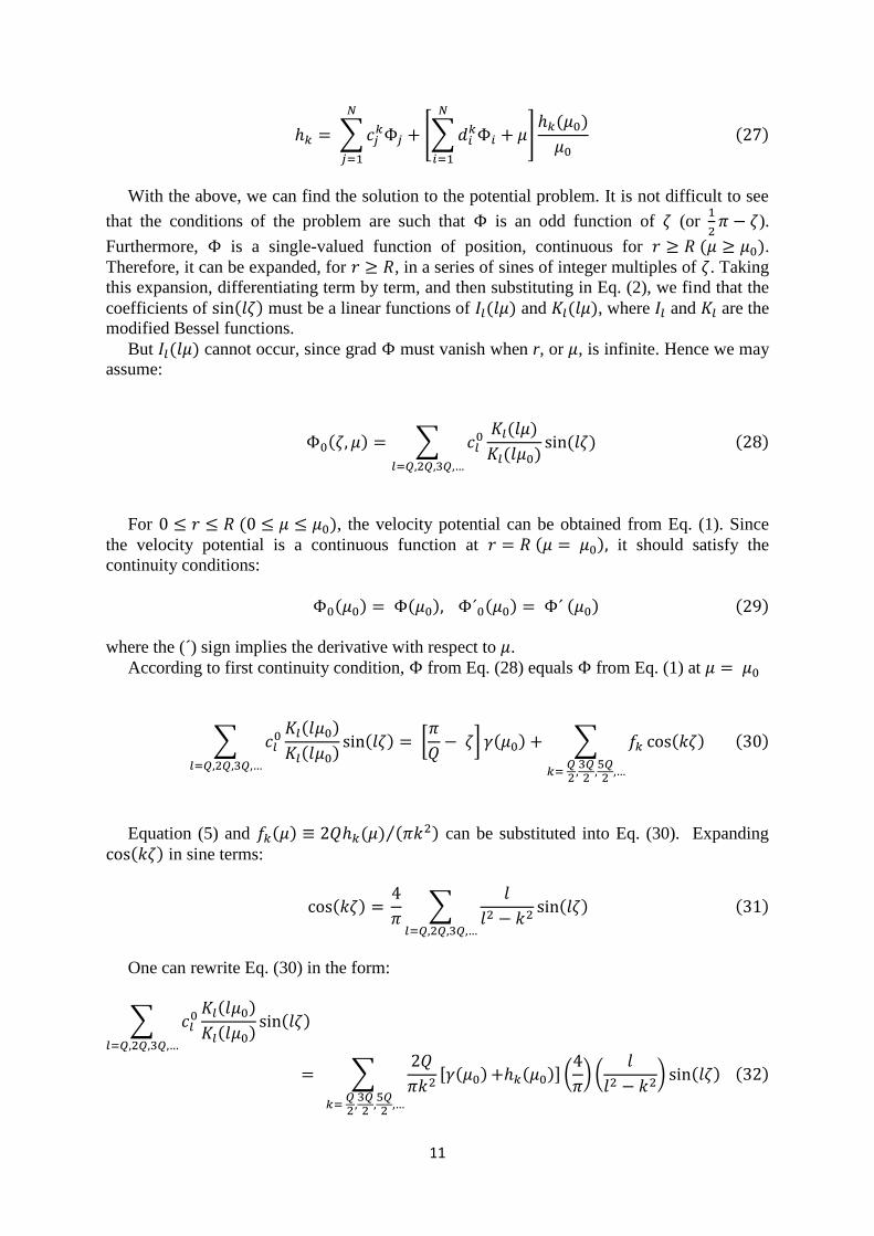
With the above, we can find the solution to the potential problem. It is not difficult to see

that the conditions of the problem are such that is an odd function of (or

).

Furthermore, is a single-valued function of position, continuous for .

Therefore, it can be expanded, for , in a series of sines of integer multiples of . Taking

this expansion, differentiating term by term, and then substituting in Eq. (2), we find that the

coefficients of must be a linear functions of and , where and are the

modified Bessel functions.

But cannot occur, since grad must vanish when r, or , is infinite. Hence we may

assume:

∑

For , the velocity potential can be obtained from Eq. (1). Since

the velocity potential is a continuous function at it should satisfy the

continuity conditions:

where the (´) sign implies the derivative with respect to .

According to first continuity condition, from Eq. (28) equals from Eq. (1) at

∑

[

] ∑

Equation (5) and ⁄ can be substituted into Eq. (30). Expanding

in sine terms:

∑

One can rewrite Eq. (30) in the form:

∑

∑

(

) (

)

12

and, as a result:

∑

(

) (

)

The second continuity condition implies that:

∑

(

) (

)

Substituting Eq. (33) in Eq. (34) and simplifying, we obtain:

∑

On the other hand, from Eq. (27), one obtains an expression for :

∑

[ ∑

] (

)

and at :

∑

|

[ ∑

|

] (

)

Taking:

∑

|

[ ∑

|

] (

)

13

one can rewrite Eq. (37) in the form:

Substituting Eq. (40) in Eq. (35), and dividing the whole equation by (to make the

matrices better conditioned) one obtains:

∑

Taking:

[ ∑

] [

]

∑

one can write Eq. (41) in the form:

and:

Now, that we have (from Eq. (17)), (from Eq. (26)), and (from Eq. (45)),

we can calculate the value of from Eq. (27). One may also calculate the Galerkin

optimum circulation, which is actually the expression inside the square brackets of Eq. (7).

∑

is the non-dimensional circulation for a case with an infinite number of blades, and

can be calculated from Eq. (6); but since the optimum Betz velocity distribution is

√ ⁄ , then would be:

14

With the Galerkin optimum circulation, one obtains the corrected circulation, , from Eq.

(48):

Where is the Prandtl correction factor Ref. [1] used to make the tip correction, and are

the solutions from the Galerkin method. In order to maximize convergence, the Prandtl

factor is used––but designed only to eliminate the residual––not correct the entire function.

We add a acceleration factor, , to account for the fact that the residual dies out more quickly

as more terms are added. The factor is chosen so as to minimize the number of terms

required for convergence in the matrix formulation. The modified Prandtl function is

therefore of the form:

With:

√

the correction factor for optimized convergence has been expressed in the following form:

(

) [

] [

]

[

] [

]

Once the solution for the corrected circulation is found, one can define the induced-power

efficiency (IPE) as the ratio of the Goldstein optimum power (for a given number of blades) to

the Glauert ideal power for an actuator disk:

∫

2.5. Results

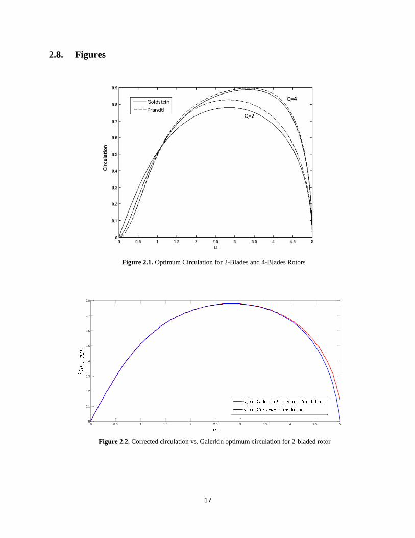
The present methodology is first used to compute cases already found in Goldstein as a

verification of the convergence and accuracy of the method. Next, results, not found in earlier

work are computed. Figures 2-4 compare the corrected circulation (circulation with the tip

correction), and the Galerkin optimum circulation (circulation without the tip correction) for

2, 4 and 6 bladed rotors. The results are for and which we found was

sufficient for convergence in all cases. Figure 2 shows our results in red for =5 and

, for which we have a known solution from Goldstein. One can see that convergence is

slow near the tip in that the zero boundary condition has not converged. Goldstein noted the

same effect with his solution; and he mentions in his paper that he adds a correction to bring

the tip to zero

15

From the singularity at the edges the convergence may be very slow. The corresponding

point in the graph may be displaced this amount if the curve can thereby be smoothed.

Goldstein

We similarly smooth the curves at the tip with our accelerated Prandtl tip-correction

function, and that is shown in the blue curve which is virtually identical to the Goldstein

solution. Figure 3 is for and , another case for which Goldstein gives a

solution. Similarly good convergence is seen. Figure 4 is for a six-bladed rotor, a result

which has not heretofore been published.

We next compute the induced-power efficiency ( ) for these cases. These are plotted

versus the Glauert tip-speed ratio (the ratio of tip speed to free-stream velocity) and also

versus its reciprocal ⁄ in Fig. 5 for rotors with 2, 4 and 6 blades.

The decreases with increasing because the local blade lift is perpendicular to the vortex

sheet and thus tilts––implying energy is lost in wake swirl. Figure 5 also shows how a

decrease in blade number reduces efficiency because there are tip losses associated with

upwash at the tip.

Figures 6, 7 and 8 compare the under various induced-flow assumptions. The curve

labeled "Betz Approximation" is the for the infinite-blade case, which includes only the

effect of lift tilt. The curve noted as "Prandtl Approx-imation" is the result of the Prandtl

blade-number correction applied to the Glauert actuator-disk model. It includes only tip

effects. The curve, "Betz-Prandtl Approximation" is the methodology suggested by Betz and

Prandtl (and implemented by Goldstein in Fig. 1) in which the Prandtl correction is applied to

the Betz solution. The final curve, labeled "Goldstein Exact Solution" is the result of our

analysis which gives the complete solution including root losses as well as tip losses. One

can see the relative effects of the various physical processes on the induced power efficiency.

Figures 6-8 reveal the magnitude of the various contributions: of lift tilt (the Glauert

curves), of tip losses (the Prandtl curves), of combined tilt and tip losses (the Betz-Prandtl

curves), and of root corrections (the exact curves). It is clear that the Betz-Prandtl

approximation gives an almost exact result for the when > 2.0, and a very good

approximation even for < 2.0. This is because the Goldstein correction, clearly seen as a

large effect in Fig. 1, has both positive and negative corrections to the Betz-Prandtl

circulation. Thus, the net effect on efficiency is small. With the new, numerical method for

finding the true Goldstein circulation, it has been possible for the first time to verify the effect

of the Betz-Prandtl approximation on induced power efficiency ( ).

2.6. Summary and Conclusions

With the use of a Galerkin procedure, we have obtained an efficient and accurate method

for solving the Goldstein optimum circulation distribution for propellers with arbitrary blade

number and tip-speed ratio. The numerical procedure is verified against results given by

Goldstein for two specific cases, and it is then used to compute results not given by

Goldstein. The results are used in order to find induced power efficiency of propellers.

These results show that the effect of Goldstein’s root corrections on are quite small such

that the Prandtl-Betz approximation is generally adequate. However, the optimum circulation

is significantly affected by Goldstein’s root effect for large wake spacing (i.e., for small blade

number and small inflow ratio .)

16

2.7. References

1. Betz,A and Prandtl, “L.,Schraubenpropeller mit Geringstem Enegieverlust,”

Goettnger Nachtrichten, March 1919, pp. 193-217.

2. Goldstein, Sydney, “On the vortex Theory of Screw Propellers,” Proceedings of the

Royal Society of London. Series A, Containing Papers of a Mathematical and

Physical Character, Vol. 123 of 792, The Royal Society, April 6, 1929, pp. 440-465.

3. Makinen, Stephen, Applying Dynamic Wake Models to Large Swirl Velocities for

optimal Propellers, Doctor of Science Thesis, Department of Mechanical and

Aerospace Engineering, Washington University in St. Louis, May 2005.

4. David A. Peters, A. Burkett and S. M. Lieb, “Root Corrections for Dynamic Wake

Models”, Presented at the 35th

European Rotorcraft Forum, Hamburg, Germany,

September 2009.

5. Szabó, Barna, and Babuska, Ivo, Finite Element Analysis, John Wiley & Sons, New

York, 1991, pp.37-38.

17

2.8. Figures

Figure 2.1. Optimum Circulation for 2-Blades and 4-Blades Rotors

Figure 2.2. Corrected circulation vs. Galerkin optimum circulation for 2-bladed rotor

0 0.5 1 1.5 2 2.5 3 3.5 4 4.5 50

0.1

0.2

0.3

0.4

0.5

0.6

0.7

0.8

18



0 0.5 1 1.5 2 2.5 3 3.5 4 4.5 50

0.1

0.2

0.3

0.4

0.5

0.6

0.7

0.8

0.9

0 0.5 1 1.5 2 2.5 3 3.5 4 4.5 50

0.1

0.2

0.3

0.4

0.5

0.6

0.7

0.8

0.9

1

19

Figure 2.5. Induced power efficiency for 2, 4 and 6 blades rotor by Goldstein’s Solution

0 2 4 6 8 10 12 14 16 18 200

0.1

0.2

0.3

0.4

0.5

0.6

0.7

0.8

0.9

1

0

Effic

ien

cy

Q=6

Q=4

Q=2

0 0.5 1 1.5 2 2.5 3 3.5 40

0.1

0.2

0.3

0.4

0.5

0.6

0.7

0.8

0.9

1

Effic

ien

cy

Q=6

Q=4

Q=2

20

Figure 2.6. Induced power efficiency, Goldstein’s Exact Solution vs. Other approximations,

2 bladed rotor

0 0.5 1 1.5 2 2.5 3 3.5 40

0.1

0.2

0.3

0.4

0.5

0.6

0.7

0.8

0.9

1

Effic

ien

cy

Betz Approximation

Prandtl Approximation

Betz-Prandtl Approximation

Goldstein's Exact Solution

0 2 4 6 8 10 12 14 16 18 200

0.1

0.2

0.3

0.4

0.5

0.6

0.7

0.8

0.9

1

0

Effic

ien

cy

Betz Approximation




21


4 bladed rotor

0 2 4 6 8 10 12 14 16 18 200

0.1

0.2

0.3

0.4

0.5

0.6

0.7

0.8

0.9

1

0

Effic

ien

cy

Betz Approximation




0 0.5 1 1.5 2 2.5 3 3.5 40

0.1

0.2

0.3

0.4

0.5

0.6

0.7

0.8

0.9

1

Effic

ien

cy

Betz Approximation




22

0 2 4 6 8 10 12 14 16 18 200

0.1

0.2

0.3

0.4

0.5

0.6

0.7

0.8

0.9

1

0

Effic

ien

cy

Betz Approximation




0 0.5 1 1.5 2 2.5 3 3.5 40

0.1

0.2

0.3

0.4

0.5

0.6

0.7

0.8

0.9

1

Effic

ien

cy

Betz Approximation





6 bladed rotor

23

Chapter 3

A COMPACT, CLOSED-FORM SOLUTION

FOR THE OPTIMUM, IDEAL WIND TURBINE

Dr. David A. Peters McDonnell Douglas Professor of Engineering

[email protected]


[email protected]


Campus Box 1185



April 4, 2012

3.1. Abstract

The classical momentum solution for the optimum induced-flow distribution of a wind

turbine in the presence of wake swirl can be found in many textbooks. This standard derivation

consists of two momentum balances (one for axial momentum and one for angular momentum)

which are combined into a formula for power coefficient in terms of induction factors.

Numerical procedures then give the proper induction factors for the optimum inflow distribution

at any radial station; and this, in turn, gives the best possible power coefficient for an ideal wind

turbine.

The present development offers a more straightforward derivation of the optimum turbine.

The final formulas give the identical conditions for the ideal wind turbine as do the classical

solutions—but with several important differences in the derivation and in the form of the results.

First, only one momentum balance is required (the other being redundant). Second, the solution

is provided in a compact, closed form for both the induction factors and the minimum power—

rather than in terms of a numerical process. Third, the solution eliminates the singularities that

are present in current published solutions. Fourth, this new approach also makes possible a

closed-form solution for the optimum chord distribution in the presence of wake rotation.

Published in the Wind Energy Journal, Feb. 6, 2013, DOI: 10.1002/we.1592



24

3.2. Nomenclature

a axial induction factor, u/U

value of a at blade tip

a' classical swirl induction factor, v/Ωr

b total induction factor, w/U

value of b at blade tip

B number of blades

c blade chord, m

blade drag coefficient

blade lift coefficient, L/[cV2/2]

turbine power coefficient, P/[πR2U

3/2]

net power coefficient

turbine torque coefficient, Q/[πR3U

2/2]

turbine thrust coefficient, T/[πR2U

2/2]

total thrust coefficient

f new swirl induction factor, v/U (a' = )

integral of power due to drag

integral of thrust due to drag

dL lift on annular ring of width dr, N

r radial position, m

non-dimensional radial position r/R

R tip radius, m

P power delivered by wind turbine, N-m/sec

Q rotor torque, N-m

u induced velocity in axial direction, m/sec

U wind velocity, m/sec

v induced velocity in swirl direction, m/sec

V total velocity relative to airfoil, m/sec (Ur of Ref. 1)

w total induced velocity (parallel to total thrust), m/sec

x Ref. 1 change of variable, x=1-3a

y present change of variable, y=3b-1

z intermediate variable, z=b2/(1+

)

blade angle of attack, rad

small quantity, << 1

blade inflow angle, rad

nondimensional total flow, V/U

local inflow ratio, Ωr/U

tip speed ratio, ΩR/U

blade pitch angle, rad

air density, kg/m3

local solidity, Bc/(2πr) (' of Ref. 1)

rotor angular velocity, rad/sec

25

3.3. Introduction

The first objective of this paper is to demonstrate that the solution for the induction factors of

an ideal optimum wind turbine (and for the resultant optimum power coefficient) can be derived

in a more direct manner than has been done in earlier derivations. The second objective of this

paper is to show that––as the result of this more direct derivation––one can obtain a set of

compact, closed-form expressions for these optimum induction factors and power coefficient.

This is in contrast to past derivations, which terminate with a numerical procedure to complete

the optimum rotor (rather than ending in compact formulas). Furthermore, because of the more

direct approach of a unified momentum theory, singularities inherent in earlier approaches are

eliminated

The third objective of this paper is the revelation that this new, direct derivation (along with

the more compact expressions) is possible because of the fact that axial momentum theory and

swirl momentum theory are redundant to each other, which implies that only a single, unified

momentum theory is necessary for the development. Finally, the fourth objective of this paper is

to show how the optimum chord and twist distributions for a rotor (including profile drag) can

also be found in closed form without the necessity of the neglect of wake swirl. It is hoped that

these compact, closed-form expressions will yield additional insights into the nature of an

optimum wind turbine.

3.4. Background

It is a well-known fact that the Betz optimum for an actuator disk (acting as a wind turbine

rotor) is that the disk slows the wind at the disk to 2/3 of its incoming value (which implies that it

is slowed to 1/3 of the incoming value far downstream). This theoretically yields 16/27 (or

59.3%) of the incoming kinetic energy converted as useful energy. However, for a disk that

generates lift and torque through lifting blades, the lift is not perpendicular to the disk. The lift

consequently creates a swirl velocity that imparts kinetic energy in the wake due to rotation. As

a result, the distribution of induced flow for optimum power with swirl is more complicated than

is the Betz solution; and the maximum possible power is smaller than 16/27.

The derivation of the optimum induced-flow distribution (including swirl)—and of the

resultant optimum power—can be found in wind turbine texts, such as Refs. [1-4]. These

derivations consist of several standard elements. First, a translational momentum theory is

performed in the axial direction in order to relate rotor thrust to the axial induced flow, u.

Second, an angular momentum theory is used to find the relationship between rotor torque and

swirl velocity, v. These momentum results are expressed in terms of an axial induction factor

and an angular induction factor (a and a', respectively) in the following form:

, (1)u aU v a r

2(1 )= (2)

(1 )r

a a

a a

26

The resulting power per unit radius can be expressed in terms of tip-speed ratio to give:

3

28 (1 ) d (3)r

PdC a a

Equation (2) can then be used to find a' in terms of a, the latter of which can then be placed

into Eq. (3). Noting that the derivative with respect to a of Eq. (3) must equal to zero allows one

(after considerable algebra) to obtain the optimality condition:

22 (1 )(4 1) (1 3 )= , (4)

(1 3 ) (4 1)r

a a aa

a a

The optimality condition in Eq. (4) can be written as a cubic in a:

3 2 2 216 24 (9 3 ) 1 0 (5)r ra a a

Although closed-form solutions exist for cubic equations, Ref. [5], the algebra is not

particularly conducive to finding a closed form for the proper root of Eq. (5). Thus, the solution

to Eq. (5) is traditionally done numerically. The final inflow angle then follows directly once the

induction parameters (a and a') are determined:

1 11tan = tan (6)

(1 )r

r

a a

a a

In order to find the total optimum induced power, Ref. [1] makes two additional changes of

variable in the integral of Eq. (3). First, a change is made from to a; and then a change is

made from a to x = 1-3a. The resultant integral for yields an expression that must be

evaluated at the upper and lower bounds to find ;

0

0.25

5 4 3 2

2

1 3

8 64 472 124 38 63 12 ln( ) (7)

729 5

x

P

x a

C x x x x x xx

where is the value of a at the tip, (i.e., at ). It should be noted that the above has

singularities both in the limit as goes to zero (the blade root) and goes to infinity.

Nevertheless, Eq. (7) gives a numerical method for finding the optimum turbine based on

momentum theory.

27

3.5. Alternative Approach

What we offer here is an alternate derivation of the parameters for an optimum turbine—

along with a resulting closed-form solution both for the optimum induced flow and for the total

power coefficient. The new formulation differs in four ways from earlier expressions: 1.) only a

single momentum balance and single induction factor is required; 2.) the optimum induction

factor is found in a compact, closed form; 3.) the total optimum power is also obtained as a

single, closed-form expression; and 4.) the singularities of earlier methods are removed.

Although the resulting optimum turbine parameters are—of course—the same with the present

method as with the previous method, the more compact results gives additional insight into the

nature of the optimum wind turbine.

The geometry of the flow is crucial to the new approach for finding the optimum induced

flow distribution. Figure 1 shows the various flow velocities as seen at the airfoil. The figure

follows the convention of Glauert, Ref. [6]. It is important to note that both momentum

considerations and vortex-tube theory show that the induced flow w and the lift vector L must be

along the same line (but in opposite directions) and that this line must be perpendicular to the

total flow relative to the blade. This implies that the induced flow completely determines the

local inflow angle . To be more specific, one can note from classical momentum developments

[i.e., Ref. [1], Eqs. (3.21) – (3.28)] that the combined vector of swirl velocity and axial velocity

form an induced-flow vector that is exactly parallel to the local lift vector (but in the opposite

direction). Reference [4] shows that the same result follows when one considers vortex-tube

theory with vorticity that is directed along the wake helix. In fact, Glauert in Ref. [6] assumes

that this must be the case for the optimum rotor. The physical basis for this simple result is that

of Newton’s laws of motion. For every action, there is an equal-and-opposite reaction; and the

force vector must be proportional to the time rate of change of the momentum vector. Thus, it is

not surprising that the induced flow and force must be opposite but parallel.

Once this factor is recognized, one can see from the geometry of Fig. 1 that—because the lift

must be perpendicular to the total flow vector at the blade (the Biot-Savart Law)—it follows that

the induced flow must be perpendicular to the local vortex sheet. Based on this observation, one

can obtain a simple relationship between the original total flow and the total flow with induced

flow based on the Pythagorean theorem.

22 2 2= + (8)V U r w

Note that Fig. 1 includes several different triangles from which one can formulate ,

, and . Based on this trigonometry, many useful identities can be found. For

example, if one draws from the meeting point of and (at the bottom of the figure) a line

that ends perpendicular to the velocity vector, then the length of that line can be expressed as

– . This equation can then be squared and solved for either or

in terms of the flow variables (a very useful result).

22 2

22( ) (9)

U U r w rwsin

U r

28

22 2

22cos( ) (10)

r U r w Uw

U r

The above relationships may also be written in terms of non-dimensional parameters (including

the overall induction factor, b = w/U):

2 2 21 (11)r b

2 2

2

1( ) (12)

1

r r

r

b b vsin

w

2 2

2

1( ) (13)

1

r r

r

b b ucos

w

Therefore, the key parameter for optimum power is the total induction factor of the induced flow,

b.

The above development offers the necessary geometric relationships to allow a derivation of

the optimal wind turbine based on a single, unified momentum balance of loads versus induced

flow, as shown below.

3.6. Momentum Theory

Reference [7] proves that momentum theory can be applied directly to a tilted lift vector to

give the same induced velocity that would be obtained from vortex-tube theory. Reference [8]

proves that an actuator-disk theory also gives the same answer as vortex theory (i.e., the exact

answer) when applied to a tilted lift vector and to a tilted induced flow vector. Therefore, in

contrast to the previous derivations which invoke both axial and angular momentum balances, it

is only necessary to look at one momentum balance for the entire lift and induced flow. That

momentum balance, when written for an annular ring, is:

2 (2 ) cos( ) (14)dL rdr w U w

This single momentum equation is all that is necessary because the swirl and axial components

of w are automatically included in the geometry of Fig. 1. A separate axial or swirl balance is

redundant. To obtain power from Eq. (14), one can write:

2 (2 ) cos( ) sin( ) (15)dP rdr w U w r

The non-dimensional coefficient can then be written in terms of ⁄ :

8 1 cos( ) sin( ) (16)P rdC b b rdr

29

At this point, there are two approaches that can be taken. In the first one, trigonometric

identities can be used to solve for in terms of ––followed by a derivative to find

the maximum power. This gives an equivalent result to Eq. (5) for the optimality condition. A

second approach is to substitute and from Eqs. (12-13) and then take a direct

derivative. After considerable algebra, this results in a different cubic equation than the one in

Eq. (5),

3 2

2

116 24 9 0 (17)

1 r

z z z

where

. This cubic equation yields a closed-form result based on Ref. [5] that

lends itself to a compact form for the optimum value of b.

2 22 1

2

1 12 11 cos cos (18)

2 3 3 1

r r

r

b

21

2

11 11 2cos cos (19)

3 3 1

r

rb

2 21 1

2 2

1 11 1 11 cos cos 3 sin cos (20)

3 1 3 1

r r

r rb

Equations (18-20) are all equivalent expressions for the optimum b. The axial and swirl

inductions are: and .

3.7. Complete Expressions

With the above closed-form expression for b, the entire optimum blade can be reduced to

simple equations. At any given radial position r, one immediately knows the appropriate

. From that , Eq. (20) gives the optimum b. One can also solve for the optimum

given b. In particular, from Eq. (17), one obtains:

1 1 2 (21)

3 1r

b b

b

Based on the optimum b, one can also write relationships between b and the inflow angle.

1 (22)

1 2cos( )b

1 3 1( ) (23)

2

b bsin

b

30

1( ) (24)

2

bcos

b

Since one can relate b to and b to , one can also relate to .

21

2

11cos (25)

3 3 1

r

r

2 2cos ( ) sin ( ) cos( ) 1 = (26)

sin( ) 1 2cos( ) tan 3 2r

Thus, Eqs. (20-26) are a complete, closed-form set of expressions of any of the optimum

parameters in terms of any of the other two. Interestingly, Eq. (26) is derived in Ref. [1]––in the

context of the optimum blade chord distribution––and can be found in their Eq. (3.9.105).

It is also interesting to compare these optimum parameters to the classic induction factors (a

and a') of conventional wind-turbine aerodynamics. This is easily done based on the geometry.

1 cos( )cos( ) = (27)

2 1 2cos( )

ba b

1 2 (28)b a

sin( ) sin( )

(29)1 2cos( )r r r

f ba

Due to in the denominator, a' is singular at r=0. The new induction parameter f, however, is

well-behaved. Based on the above, one can write a compact expression for the total flow at the

blade in terms of b.

2

2 2 21

1 (30)3 1

r

b bb

b

This completes the expressions for the closed-form optimum blade parameters. Note that, at the

root, = 0, we have b = 1/2 and = 60˚. Another interesting point to interrogate is (the

point at which the original inflow angle = 45˚). There, we have b = 1/ (1+√ ) = 0.366 and =

30˚. In the limit as approaches ∞, we have b = 1/3 and = 0˚.

31

3.8. Optimum Power Coefficient

With the optimum blade parameters in compact form, it now remains to compute the optimum

(i.e., maximum) power coefficient that goes with these parameters. Based on Eq. (16), the

incremental optimum power is given by:

22

2

2(1 ) (1 2 ) 2(1 ) (1 2 ) (31)r r

P

b b ddC b b rdr

The task is to integrate this in closed form from = 0 to = 1 (or, alternatively, from to

. Since we have no closed-form expression for b in terms of , our formula for in

terms of b, Eq.(21) makes a b-integration more tractable. A differential of Eq. (21) leads to:

2

2

6 1 2 (32)

3 1r r

b bd db

b

Therefore, we can write a formula for the total in terms of a b integral.

0

2

2

0.5

12 (1 2 )(1 ) (33)

(3 1)P

b

b b bC db

b

where 0.5 is the value of b at the blade root, and is the value of b at the blade tip,

( ⁄ ⁄ ). Because of the singularity in the denominator, it is advisable to make a

change of variable to y = 3b – 1. The term can also be expressed in terms of and,

therefore, in terms of – . The resultant integral for is:

1

0

2

20

2

0 0

4 43 9 2 (34)

27 4 1 2P

y

y

yC y y dy

yy y

where = 1/2 and 0 < < 1/2.

Equation (34) can be integrated in closed form. Because each integral term involves either

ln( ⁄ ) or

, one can factor out ( ) or, equivalently, factor out (1 – ). In fact,

the cube can be factored out, . In addition, the on the outside of the integral cancels

all terms in the denominator. This then creates a term of the form which removes

the singularities from the final expression. The closed-form result for becomes:

32

2

32

3

1ln(2 ) (1 2 ) (1 2 )

1 2 216 457 51 31 (35)

27 1280 640 160 2 (1 2 )1

4

P

y y y yy y

C y yy y

For convenience, we have dropped the subscript on such that y = – 1. Note that, for y

= (1 –)/2, the term [ln(1-) + +2/2]/3

approaches -1/3, such that the formula is well-behaved.

Similarly, at y = (i.e., approaching ), ln() approaches zero such that the formula gives

the Betz limit, 16/27. Since is known in closed form in terms of , Eq.(35) is the first closed-

form expression for optimum that has been published.

3.9. Torque and Thrust Coefficients

The power coefficient in Eq. (35) goes to zero as goes to zero, this reflects the fact that, in

the limit as Ω goes to zero, there can be no power generated. However, there can be a torque in

the limit as Ω approaches zero. Since P = QΩ, the torque coefficient comes immediately from

the power coefficient.

3 3= = (36)

4 1 2

PQ P

yCC C

y y

It follows from Eq.(35) that:

2

32

3 3

1ln(2 ) (1 2 ) (1 2 )

28 3 457 51 31 (37)

9 1280 640 160 2 (1 2 )1

4

Q

y y y yy y

C y yyy

Thus, approaches 0.8653 as approaches zero. On the other hand, as approaches infinity,

goes to zero.

In a similar manner to the computation of power coefficient, one can also compute a closed-

form expression for the thrust coefficient of the optimal rotor. From momentum theory, Eq. (14),

the relationship for thrust is:

2 2 cos( ) cos( ) (38)dT rdr w U w

From this, the elemental thrust coefficient for the optimum rotor is:

2

2

2 18 1 cos( ) cos( ) = (39)

r r

T

b ddC b b rdr

33

With the change of variable into a b integral, we have:

0

2 2

22

0.5

1 2 112= (40)

3 1T

b

b b bC db

b

As with the power integral, a change of variable to y = 3b – 1 yields a closed-form expression

for the thrust of an optimum rotor.

2 3

2

1ln 2 1 2

8 55 17 1 4= 1 (41)768 192 64 1 29 1

4

T

y y y

C y y yy y

Note that, for small , it follows that y = (1 –)/2, where is a small quantity. In the limit as

approaches zero, [ln(1 – ) + ]/2 = -1/2. Also, as approaches , y =, the limit of ln() = 0.

Thus, at = 0 (y=1/2), we have =0.75; and, as approaches infinity, y=0, we have = 8/9.

3.10. Optimal Chord and Pitch

The above derivation gives the induction factor for maximum power output. It is natural to

ask as to the chord distribution and pitch angles that would give this optimum induced flow and

power––under the assumption that each blade section is operating at the angle of attack that

gives the maximum lift-to-drag ratio for that section. Section 3.9, Eq. (3.106), of Ref. [1]

gives without proof the optimum chord distribution (including swirl). In terms of our variables,

the result is.

81 cos( ) Ref.1 (42)

l

rc

BC

The equivalent result can be obtained under the present approach with the use of single

induction factor. In particular, because the lift from momentum theory (as well as the resultant

induced flow) lies along the same axis as does the lift from blade-element theory, we may write:

22 22 cos( ) 2 (43)2

l

BcdL w U w rdr U r w C dr

The balance of momentum and blade-element lift (in terms of nondimensional variables) is:

2 28 1 cos( ) (1 ) (44)l rr b BcC b

34

The parameters in Eq. (44) are known from Eqs. (20 – 30). This allows us to solve for the

optimum chord in terms of known quantities.

2

2

3 14 16 1 (45)

1l l r

br rbc

BC b BC

Equations (21-26) can be used to shown that Eqs. (42) and (45) are identical. A comparison of

Eq. (45) with similar equations that neglect swirl (i.e., Eq. (3.79) of Ref. [1]) shows that the two

expressions for chord agree for large , which is the case for which swirl is negligible.

However, results without swirl give an infinite solidity near the blade root ( = 0); whereas the

formula that includes the effect of swirl is well-behaved in Eq. (45).

There are two interesting aspects of Eq. (45). First, near the blade root, the local solidity that

results from the optimum chord is:

2

8 1 2 2 (46)

2 l l

Bc

r C C

For a typical of 1.0, this implies a solidity of 2 which would seem to be physically impossible

(the area of blades exceeds the area of the annular ring). However, near the root, = 60˚ and

. Therefore, projection of the blade chord onto the rotor disk would exactly

equal the available area; and the rotor would not interfere blade-to-blade. Another interesting

aspect of Eq. (45) is that the ideal blade has a maximum chord that is approximately located

at . For example, for , the maximum would come roughly at 14% distance

from the rotor center and would give a local solidity of around 1.0—still free from blade

interference. This also is the location at which , and the local inflow angle is 30˚.

The optimum pitch angle follows directly from the relationship that the angle of attack is

given by . Since is known in closed form from Eq. (25), and since the angle of

attack for maximum is known for each turbine airfoil, it follows that the optimum pitch

angle is known and is given by . In summary, the use of a single momentum

balance—with all else following from geometry—gives a closed-form solution for the optimum

rotor and allows computation of the optimum chord and pitch angle.

3.11. Effect of Profile Drag

It is quite straightforward to determine the effect of profile drag on the thrust, power, and

efficiency of the optimum wind turbine. This is possible because the above derivation of the

optimum rotor is based on a momentum theory and a blade element theory that both assume lift

perpendicular to the vortex sheet. Since the profile drag is by definition along an axis parallel to

the vortex sheet, it is easily included in the blade loads. What further simplifies the computation

is the fact that profile drag does not affect momentum theory. This is because only the

circulatory lift trails vorticity that creates induced flow. Profile drag may heat the air and

produce a shear layer behind each blade; but these effects are negligible in terms of their

influence on induced flow.

35

Thus, since it is specified that the local drag is perpendicular to the local lift (and has no effect

on the momentum induced flow), we may write the net elemental thrust coefficient (due to both

lift and drag) as a quantity that is proportional to:

cos( ) sin( ) cos( ) 1 tan( ) (47)dl d l

l

CC C C

C

Similarly, the elemental power coefficient is proportional to:

sin( ) cos( ) sin( ) 1 cot( ) (48)dl d l

l

CC C C

C

It follows that the existing integrals for and can be augmented with integrals that multiply

( ) in order to obtain the desired effect of drag on thrust and power.

In order to obtain insight to the effect of profile drag, we consider the case in which all airfoil

sections have the same maximum lift-to-drag-ratio along the blade span. (Of course, this does

not imply that each section has the same lift and drag.) Although a production wind turbine

generally would not have all airfoils operating at the same lift-to-drag ratio, here we are

considering only the ideal turbine. Thus, it is instructive to consider an ideal turbine with the

same airfoil geometry at all sections (and thus the same optimum lift-to-drag ratio). This allows

a closed-form expression for the effect of drag on the ideal optimum. It is not, strictly-speaking,

the optimum for a case with drag. However, since the effect of profile drag is assumed a

correction factor, one would expect the optimum induction factors not to change drastically due

to the presence of drag. Thus, this approach should yield important insight.

According to Eqs. (47) and (48), the integral for thrust or power can be multiplied by either

or , respectively, in order to obtain the integrals that are to go with in

and , respectively. The integral for due to is of the form:

0

32

2

32

2

0.5

1 2 112 (49)

3 1T

b

b b bThrust Integral I db

b

The integral for the effect of drag on is of the form:

0

322

2

52

2

0.5

1 2 1 112 50

3 1P

b

b b b bPower Integral I db

b

These integrals have been worked out in closed form. The thrust integral is:

36

3 2 2

2

4 1 4 8 1 84

6 3 3 3 33 4 1 2T

yI y y y y y

yy y

2

4 3212ln (51)

322 4y y y

The singular term at y = 0.5 ( = 0) can be factored, giving:

2

2

1 2 11 (1 2 )

32 41 994 9 48

46 3 4 1 2

lny

yy y y

y y y y yT y y

I

218 4 45 32 8 ( 4)107 64+ (52)

2 33 3 3 436 113 38 16 9 7 2 ( 4)

y y y y y y y

y yy y y y y y

The power integral becomes:

4 3 2 2

2 2

4 4 17 133 89 104 16 13 4

15 15 45 9 9 99 3 4 1 2P

yI y y y y y y

y yy y

2( 2) 4 1023

8ln (53)4 80

y y y

It turns out that this integral is nearly linear with and can be approximated by:

16 (54)

27PI

Or to make the formula a little more accurate, one can use:

3

2

27 32 (55)

54(1 )PI

The maximum error of Eq. (54) is 0.024 (at = 0.7) and that of Eq. (55) is 0.022 (at = 1.1).

These errors are, respectively, about 6% and 3% of the local integral. For all values of , Eq.

(55) gives lower errors than does Eq. (54). For example, the relative errors at = 5.0 are 0.011

37

and 0.007 respectively (0.37% and 0.24%); and the errors at = 0.2 are 0.016 and 0.004 (12%

and 3%).

From this, the integrals for the total thrust coefficient and the net power coefficient

follow directly:

[ . 41 ] (56)dTT T T

l

CC C Eq I

C

[ . 35 ] (57)dPN P P

l

CC C Eq I

C

3.12. Numerical Results

The present closed-form results are consistent with past results, but it is nonetheless

informative to plot these optimum parameters based on the formulas herein. Figure 2 presents

the three induction factors (b, a, f) versus the local speed ratio, . The total induction factor b

varies from 0.5 at to 0.33 for >> 1. The axial induction factor a varies from 0.25 to

0.33 over the same range. The swirl induction factor f shows a wider range of values, beginning

at √ ⁄ and going to zero. Figure 3 shows the total inflow angle through this same range. The

optimum angle is 60˚ for small , drops to 30˚ at = 1, and approaches 0 as becomes large.

Figure 4 plots the same data against 1/(1 + ) which is the square of the sine of the initial air-

flow angle (before the optimum induced flow is added). Thus, small inflow ratios are at the right

( tending to infinity) and large inflow ratios on the left ( tending to zero). Note that this

curve is antisymmetric about = 1 and = 30˚. This is a consequence of the closed-form result

in Eq. (25). Figure 4, therefore, is a universal curve that shows how the optimum inflow ratio

varies from 0º to 60º over the entire inflow-ratio range. A turbine with a given tip radius and

root cut-out would have optimum values of the inflow angle as found from the appropriate range

of 1/(1 + ) in the figure.

Figure 5 shows a comparison between the approximate optimum chord formula (in which

wake swirl is neglected) and the exact, closed-form result presented here. Results are for = 7,

B=3, and . Note that the root solidity is infinite for the approximate method but is well-

behaved for the true optimum.

Figure 6 presents the from the closed-form result in Eq. (35). We have verified that this

result agrees exactly with the numerical solution in Ref. [1]. This figure gives an understanding

as to why typical, production wind turbines have tip-speed ratios between 5 and 7. Values of

that magnitude are needed to approach ideal efficiency, but larger values do not yield much extra

power. Figure 7 shows the torque coefficient for the same case. Note that, for a stopped rotor,

= 0, there can still be a torque due to the lift on the blades in the free-stream. As rotor tip-speed

becomes large, less and less torque is required to produce the same optimum power; and

approaches to zero. Figure 8 gives the closed-form thrust coefficient for the optimum rotor. It

varies between 3/4 and 8/9 in a monotonic fashion.

Figures 9 and 10 give the optimum power and thrust including the effect of profile drag for

the cases = 0.00, 0.01, 0.02, and 0.04 and = 1.0. Notice that, with profile drag, a given value

of implies an optimum tip-speed ratio for maximum power. The maximum for =

38

0.04, is 0.475 (at = 2.85). For = 0.02, the maximum = 0.514 (at = 3.85). For

= 0.01, the maximum = 0.541 (at = 5.21). From this, one can infer an approximate

formula for the that gives maximum .

2

2 0.128 0.128 0.559 (58)l l l

d d d

C C C

C C C

This sheds further insight as to why typical wind turbines with high have tip speeds of

the order of 5 to 7. Note that the effect of the profile drag becomes more pronounced at high tip-

speed ratios.


An alternate derivation is provided for the parameters of an optimum, ideal wind turbine, Unlike

previous derivations, only a single momentum theory is used (in the direction of the local lift) so

that there are no separate accounts of axial and angular momentum. The results, also unlike

previous results, are found in closed form for all variables—and the singularities of previous

numerical solutions are eliminated explicitly. Although the final parameters for the optimum

turbine are no different from those of conventional approaches, the closed-form nature of the

results yields insight into the properties of the optimum turbine. Finally, because of the single

momentum balance, it is quite straightforward also to write a closed-form expression for the

optimum blade chord distribution. The true optimum does not become singular at the blade root,

but rather approaches a combination of solidity and pitch angle that avoids blade-to-blade

interference.

3.14. References

1. Manwell, J. F., McGowan, J. G., and Rogers, A. L., Wind Energy Explained: Theory,

Design and Application––Second Edition, John Wiley and Sons, West Sussix, 2009, pp. 91-

101, 117-123.

2. Johnson, Gary L., Wind Energy Systems, Prentice-Hall, Englewood Cliffs, NJ, 1985,

pp. 124-136.

3. Eggleston, David M. and Stoddard, Forrest S., Wind Turbine Engineering Design,

Van Nostrand Reinhold Company, New York, 1987, pp. 15-29.

4. Garcia-Sanz, Mario and Houpis, Constantine H., Wind Energy Systems, CRC Press,

Boca Raton, FL, 2012, pp. 81-292.

5. Abramowitz, Milton and Stegun, Irene A., Handbook of Mathematical Functions,

Dover Publications, Inc., New York, NY, 1970, p. 17.

39

6. Glauert, H., Aerodynamic theory: A General Review of Progress, Vol. IV, Chapter

Division L., Airplane Propellers. Dover Publications, Inc. New York, NY, 1963, pp.

169-368.

7. Barocela, Edward, "The Effect of Wake Curvature on Dynamic Inflow for Lifting

Rotors," Master of Science Thesis, Washington University in St. Louis, May 1997.

8. Makinen, Stephen M., Applying Dynamic Wake Models to Large Swirl Velocities for

Optimum Propellers, Doctor of Science Thesis, Washington University in St. Louis,

May 2005.

40

3.15. Figures

Figure 3.1. Rotor Inflow Geometry

41

Figure 3.2. Wake Induction Parameters as a Function of Local Speed Ratio

Figure 3.3. Optimum Inflow Angle as a Function of Local Speed Ratio

0 1 2 3 4 5 6 7 8 9 100

0.05

0.1

0.15

0.2

0.25

0.3

0.35

0.4

0.45

0.5

r

a,b

,fFigure 2. Wake Induction Parameters as a Function of Local Speed Ratio

a (Axial Induction Factor)

f (Swirl Induction Factor)

b (Total Induction Factor)

0 1 2 3 4 5 6 7 8 9 100

10

20

30

40

50

60

r

Figure 3. Optimum Inflow Angle as a Function of Local Speed Ratio

42

Figure 3.4. Optimized Inflow Angle as a Function of of Initial Inflow Ratio

Figure 3.5. Optimum chord, theory with wake rotation vs. theory without wake rotation

(

0 0.1 0.2 0.3 0.4 0.5 0.6 0.7 0.8 0.9 10

0.05

0.1

0.15

0.2

0.25

0.3

0.35

0.4

Nondimensionalized blade radius, r/R

Nondim

ensio

naliz

ed b

lade c

hord

, c/R

Figure 5. Optimium Chord, Theory with Wake Rotation vs Theory without Wake Rotation, = 7, Cl = 1, B = 3

Theory without Wake Rotation

Theory with Wake Rotation

43

Figure 3.6. Power Coefficient as a Function of Tip Speed Ratio

Figure 3.7. Torque Coeficient as a Function of Tip Speed Ratio

0 1 2 3 4 5 6 7 8 9 100

0.1

0.2

0.3

0.4

0.5

Cp

Figure 6. Power Coefficient as a Function of Tip Speed Ratio

0 1 2 3 4 5 6 7 8 9 100

0.1

0.2

0.3

0.4

0.5

0.6

0.7

0.8

0.9

CQ

Figure 7. Torque Coefficient as a Function of Tip Speed Ratio

44

Figure 3.8. Thrust Coefficient as a Function of Tip Speed Ratio

Figure 3.9. Power Coefficient as a Function of Tip Speed Ratio Including the Effect of Profile Drag

0 1 2 3 4 5 6 7 8 9 100.75

0.8

0.85

0.9

CT

Figure 8. Thrust Coefficient as a Function of Tip Speed Ratio

0 1 2 3 4 5 6 7 8 9 100

0.1

0.2

0.3

0.4

0.5

0.6

0.7

CP

N

Figure 9. Power Coefficient as a Function of Tip Speed Ratio Including the Effect of Profile Drag

Cd / C

l = 0.00

Cd / C

l = 0.01

Cd / C

l = 0.02

Cd / C

l = 0.04

45

Figure 3.10. Thrust Coefficient as a Function of Tip Speed Ratio Including the

Effect of Profile Drag

0 1 2 3 4 5 6 7 8 9 100.75

0.8

0.85

0.9

CT

T

Figure 10. Thrust Coefficient as a Function of Tip Speed Ratio Including the Effect of Profile Drag

Cd / C

l = 0.00

Cd / C

l = 0.01

Cd / C

l = 0.02

Cd / C

l = 0.04

46

Chapter 4

OPTIMUM PERFORMANCE OF AN ACTUATOR DISK BY

A COMPACT MOMENTUM THEORY INCLUDING SWIRL


David A. Peters McDonnell Douglas Professor of Engineering




October 13, 2012

4.1. Abstract

A new compact form of momentum theory is introduced for actuator disks including swirl.

The new form unifies both the axial and angular momentum balances into a single momentum

equation, applicable over the entire range of thrust and power coefficients. While completely

consistent with earlier momentum theories, such as that of Glauert in Ref. [1], the compact form

allows analytic expressions for the parameters of an optimum actuator disk and reveals

additional insight into the limiting efficiency of rotors, propellers, and wind turbines. Closed-

form results presented here include the optimum values of: induced flow, inflow angle, thrust,

induced power, and efficiency. Closed-form expressions are also given for optimum twist, chord

distribution, and solidity in the presence of profile drag (along with the resulting over-all

efficiencies). For the limiting case of the optimum rotor in hover, the compact form leads to

closed-form expressions for both contraction ratio and pressure distribution in the far wake. This

report also gives a formal proof that the Betz inflow distribution results in the maximum figure

of merit, and it further demonstrates that some approximations used in earlier actuator-disk

momentum theories have been inconsistent.

Presented at the AHS 69th Annual Forum, Phoenix, Arizona, May 21–23, 2013.

47

4.2. Nomenclature

b blade number

c blade chord, m

Cd local blade drag coefficient

Cl local blade lift coefficient

CP rotor power coefficient, P/(πR2Ω

3R

3)

CPG Glauert minimum power

CPI minimum induced power

CPT total power, induced power plus profile power

CT rotor thrust coefficient, T/(πR2Ω

2R

2)

CTN net thrust coefficient, lifting thrust less drag download

mapping from to :

swirl-loss function, Eq. (A6)

FL reaction force on lower momentum tube, N

FU reaction force on upper momentum tube, N

axial drag integral, Eq. (A11)

inplane drag integral, Eq. (A12)

contraction ratio, ⁄ √ ⁄

L local lift, N

P rotor power, watts

PC normalized pressure required to balance centrifugal force, N/m2

PW normalized pressure in far wake for consistent momentum theory, N/m2

r nondimensional radial coordinate, x/R

nondimensional radial coordinate in far wake, ⁄

normalized radial coordinate, r/( + 0)

R rotor radius, m

radius of wake far downstream, m

T rotor thrust, N

u axial flow at airfoil, m/sec

normalized axial velocity,

axial induced flow in far wake, m/sec

normalized axial velocity, ⁄

U rotor climb rate, m/sec

local air speed relative to airfoil, m/sec

V dynamic-inflow mass-flow parameter, ( + 2 0)

VT dynamic-inflow total-flow parameter, ( + 0)

w local induced flow, parallel to L, m/sec

nominal value of ideal inflow extrapolated to r =

x radial coordinate, m

radial coordinate in far wake, m

local blade angle of attack, – , rad

total circulation on all blades at a radial position, m/sec2

nondimensional circulation, /(2πΩR2)

48

local inflow angle, rad

blade pitch angle, rad

nondimensional local flow,

nondimensional climb rate, U/(ΩR)

nondimensional induced flow, w/(ΩR)

nondimensional nominal induced flow, w0/(ΩR)

air density, kg/m3

blade solidity, (blade area)/πR2

projected (i.e., weighted) solidity, [projected area]/(πR2)

rotation rate of flow just below disk, rad/sec

rotation rate of flow in far wake, rad/sec

normalized wake rotation, /Ω

normalized wake rotation in far wake, 1/Ω

Ω rotor angular speed, rad/sec

IPE induced power efficiency, CPG/CPI

TRE total rotor efficiency, CPG/CPT

4.3. Background

It is well-known that the optimum induced flow distribution for a lifting, actuator disk is a

uniform pressure and (consequently) a uniform induced-flow distribution, Ref. [1]. This is the

loading and inflow that give the minimum power for a specified thrust (or, equivalently, the

maximum thrust for a given power). However, a rotor system is not a true actuator disk (i.e.,

does not have a loading perpendicular to the disk). Rather, the local lift of a rotor is

perpendicular to the vortex sheet coming off of the blades; and the resulting tilt of the lift results

in a swirl velocity with loss of energy.

Betz postulated from vortex considerations that the optimum inflow distribution is one that

causes the vortex sheet to come off of the blades along a prescribed helix, Ref. [2]. He specifies

the circulation distribution necessary to obtain that ideal inflow for the case of a lightly-loaded

rotor with an infinite number of blades. In that same work, Prandtl gives an expression for an

approximate correction for the circulation distribution that would result in this optimum induced

flow for the case of a finite number of blades. Goldstein, Ref. [3], provides an exact solution for

the circulation distribution that results in the optimum Betz inflow for a lightly-loaded rotor with

a finite number of blades. Goldstein also demonstrates that the Prandtl approximation is quite

accurate.

Reference [1] also uses the Betz optimum loading distribution––specialized to the case of

hover with an infinite number of blades––to work out some numerical calculations for the

optimum figure of merit for a lifting rotor. This is done for small thrust coefficients, for which the figure of merit lies between 1.0 and 0.89. The results offer a valid

representation of how figure of merit is affected by wake swirl. However, a general formula for

rotor efficiency as a function of climb rate (and valid for all thrust levels) has not been worked

out. It would be beneficial to have such an expression (at least for an infinite number of blades).

For such a solution to be generally useful, it should be valid throughout the entire range of rotor

loadings from a lightly-loaded propeller to the case of a helicopter in hover. A result such as this

49

would give insight into the nature of optimum rotors and could provide a benchmark against

which to compare optimization routines coupled to comprehensive codes. Presumably, the effect

of a finite number of blades could be accounted for by the Prandtl approximation applied as a

correction.

The purpose of this paper is to describe the optimum lifting rotor in terms of the optimum

inflow distribution (as well as the optimum twist and chord that would result in such a

distribution), and to find the resultant thrust, power, and efficiency of the optimum rotor as

compared to the Glauert ideal for an actuator disk. Results are provided in a compact, closed

form that yields insight into the nature of optimum rotors throughout the range of operating

conditions. In addition, these results are compared with other references who have treated the

problem; and a formula is derived for the optimum contraction ratio. A summary of the main

results is given in Appendix A.

4.4. Geometry of Optimum

Figure 1, taken after Ref. [2], shows the geometry of the flow field at a typical blade section.

In the figure, Ωx is the air velocity from blade rotation, U is the air flow due to the climb rate of

the rotor (positive for a rotor moving through the air in the same direction as the rotor lift), and w

is the induced flow at the blade. This figure is valid for all cases––from a lightly-loaded

propeller to a helicopter in hover or a lifting fan. Notice that the local lift L and the local induced

flow are parallel (but in opposite directions) to each other and that they both are perpendicular

to the local flow velocity, u. This is a direct result of the physics of the situation and follows

either from application of vortex theory or momentum theory. As a consequence of this

geometry, the local velocities and the inflow angle are completely determined in terms of the

rotational speed Ωx, the climb rate U, and the local induced flow magnitude , as shown below.

√

√

The velocity noted in Fig.1 as w/cos() is a construct in the geometry of the figure and is not a

physical velocity in the system. Nonetheless, it is a useful construct in order to express the

geometry. It is important to note that the induced velocity w has a vertical component wcos()

that adds to U and a swirl component wsin() that subtracts from Ωx.

Betz proved that the optimum induced flow distribution w(x) is one that remains along a helix

as it leaves the rotor disk. In other words, the optimum distribution has the form:

50

where is the local inflow angle and w0 is a nominal velocity that equals the inflow velocity

extrapolated to an infinite radius, cos() = 1.0. The use of w0 in this parametric way makes it

very convenient to express the optimum rotor for any condition in terms of this free parameter

w0. It is also convenient to express all quantities as normalized on the tip speed, ΩR. Thus, we

define the normalized velocities:

With these definitions, the optimum induced flow and inflow angle become:

√

(

)

√

√

√

These are the parametric equations define the inflow for an optimum lifting rotor.

4.5. Momentum Theory

To find the resultant thrust and power of the Betz optimum inflow distribution requires an

inflow theory that relates loading to w. For the lightly-loaded theory of Goldstein, Ref. [3], one

can use a potential-flow, vortex model; but, for the case of finite loading, momentum theory is

the model of choice. To include swirl velocity in the analysis, one would normally do both an

axial and an angular momentum balance––as is done for the inflow of wind turbines, Ref. [4].

However, two balances are not necessary because angular momentum theory is redundant to

axial momentum theory due to the fact that the total induced flow must be along the same axis as

the local lift, Fig. 1.

Reference [5] specifically demonstrates that––when one takes the tilted lift that is on the

blade but then applies that lift perpendicular to a notional, actuator disk (computing the axial,

momentum-theory inflow perpendicular to that notional disk)––this computed induced flow is

identical to the skewed inflow at the actual blade due to the tilted lift as determined by either

vortex-tube theory or a combination of axial and angular momentum theory. Similarly, Makinen

Ref. [6] shows that, when applied in this way to a lightly-loaded rotor with wake swirl and a

finite number of blades, actuator-disk theory gives the same optimum induced flow distribution

as found by Goldstein. Thus, it is completely rigorous to apply a single momentum balance

along the lift direction in order to give both axial induced flow and the swirl flow.

51

Reference [7] sets out the general theory of how this might be done and works out some

closed-form results in hover when the effect of drag on lift is neglected. In this work, we follow

the approach of Ref. [7] and apply a single momentum balance in order to determine the

optimum lifting rotor. This balance reflects that the local lift is equal to the mass-flow rate

across the disk multiplied by the change in induced flow which is along the same direction as the

lift (and which doubles downstream). This process results in a general momentum balance for an

annular ring on the disk, as follows:

From this, the incremental thrust (normal to the disk) and the incremental power are:

The nondimensional forms follow from the definitions given earlier.

From the integrals of these expressions, one can find the thrust and power for any induced flow

distribution––including the effect of swirl. Equations (11) - (14) are also applicable to wind

turbines, for which and (and, consequently, thrust and power) would be negative.

When the optimum values of and from Eqs. (6-8) are placed into Eqs. (13-14), one has the

thrust and power for the particular case of the optimum lifting rotor.

Note that each elemental power in Eq. (15) is proportional to a corresponding elemental thrust in

Eq. (16): . Furthermore, since CT is the useful work done by the rotor, it

follows that the incremental induced power is given by:

Equations (15-17) can be integrated to determine the total thrust and power. The integrand of

each of these integrals is identical. This is not simply a coincidence, but it is the natural

consequence of having chosen the Betz optimum induced-flow distribution. The kernel integral

of these coefficients is defined here as the swirl-loss function f(, 0) and is given by:

52

∫

Appendix B works out this integral in closed form, and it is:

[

]

This function is unity for a rotor at high tip speeds (small ) and decreases as tip speed becomes

smaller (large ). It is interesting that this function depends on the same two key parameters as

does dynamic inflow theory, V = ( + 2 0) and VT = ( + 0).

4.6. Induced Power and Efficiency

With the above, one may write the thrust and power integrals in closed form as:

The form is reminiscent of the relationship for the Glauert ideal case of uniform

flow in which However, here is not uniform inflow but is rather the extrapolation of

the optimum flow field off of the disk to where it would approach uniform flow. Thus, is

greater than the induced flow anywhere on the disk; and the required induced power is greater

than the Glauert minimum. Equations (19-22) give closed-form expressions for the thrust,

power, and induced power of an optimum rotor that is loaded. They are written in terms of the

climb rate and the parameter ––which is the nominal flow extrapolated to infinity. A

lightly-loaded rotor is the case of << 1.

It is instructive to look at the induced power efficiency (IPE)––which is the minimum Glauert

power for an actuator disk divided by the true induced power of the lifting rotor. The minimum

Glauert power can be obtained by setting in Eqs. (20) and (22), and then solving for

in terms of . This is, by definition, .

[ ⁄ √ ⁄ ⁄ ]

⁄

⁄ √ ⁄ ⁄

The induced power efficiency follows directly from Eqs. (22) and (24):

53

⁄

√

This can be written in terms of and by use of the formula from Eq. (20).

√

Equation (26) is the closed-form expression for induced power efficiency for lifting rotors at all

operating conditions.

It is interesting to look at some special cases of Eq. (26). The case of a lightly-loaded rotor is

given by setting .

(

)

The case of hover is found by setting = 0.

√

√

⁄

√

√ √

(

)

Equations (27-28) are identical to the formulas derived in Ref. [7]. Eq. (28) is the figure of merit

(due to induced losses) for a hovering rotor.

Another interesting case is the limit as becomes large. In this limit, the angle of the

vortex sheet approaches 90º. The resultant thrust and induced power then become:

[

⁄

]

Equation (29) implies that approaches zero for large . Thus, does not increase

monotonically with but rather reaches a maximum and then tends to zero as increases

further. Induced power ( ), on the other hand, approaches the value of for large and goes

to zero only for the case of hover ( = 0). In hover, thrust reaches the maximum value ( =

0.238) at = 0.78; and, although both and tend to zero with large , the induced power

efficiency (i.e., figure of merit) decreases monotonically as increases––with a limit of zero.

The above formulas thus give a complete description of the optimum rotor in hover.

54

4.7. Shape of Optimum Rotor

While the above formulation gives the induced flow distribution and the resulting thrust and

power coefficients for the optimum rotor, it is interesting to ask what the blade shape would be

for such an optimum rotor. First, consider the form of the optimum twist distribution. It is

assumed that the optimum rotor would be one for which the angle of attack is set at

the fixed point for the maximum ⁄ at each blade section. Based on Eq. (6), it follows that

the optimum blade twist would be given by:

(

)

where is the angle of attack for minimum ⁄ .

The optimum chord for the rotor follows directly from the fact that the at every blade

station is fixed at the optimum . From blade-element theory, this implies that:

(

)

where b is the number of blades and c is the local chord. Blade-element lift––like momentum-

theory lift––must be perpendicular to the vortex sheet. Therefore, Eq. (31) can be set equal to

Eq. (10) in order to solve for the chord that will give the optimum induced flow .

The resultant value for the normalized blade chord is:

(

) [

√ ]

This is the closed-form result for the optimum chord distribution.

It is also useful to present this result in terms of the local projected solidity (blade area

projected on an annular ring divided by the ring area 2πrdr).

(

) (

) (

) [

]

The total projected solidity (analogous to the weighted solidity often used in helicopter

design) can be found directly by integration of ⁄ from Eq. (33).

(

)

[

] (

) [

]

It is instructive to study the nature of the chord distribution (and projected chord distribution)

in hover ( = 0). There, Eqs. (32-33) become, respectively:

55

(

) (

)(

√

)

(

) (

)(

)

The true solidity and the projected solidity in hover are, respectively:

(

) (

√

) (

)

(

)

In illustration of the above, consider = 0, = 0.1 and = 1.2. The various optimum

values for this case are given in Table 1. The resultant solidities for this case are = 0.20 and = 0.15. Despite these reasonable solidities, the chord in this blade becomes large as r approaches

zero. The relationship in Eq. (35) yields a condition at r = 0, of ⁄ ⁄

(or ⁄ ) which would be impractical. However, one cannot truly continue any blade

all the way to r = 0 (since there must be a hub); and the root section for this case (r < 0.1) has

little effect on the total thrust or power. Thus, the chord very near the hub is not of practical

consequence. The projected chord, on the other hand, goes to zero at the blade root; and the

maximum projected chord in this example (near r = = 0.1) is given by ⁄ .

The local projected solidity at the annular ring (i.e., the location r = 0.1) is consequently

⁄ ⁄ , implying some nominal overlap of blades––but no blade-to-

blade interference.

It is also interesting to examine the blade projected chord distribution and solidity for the case

of the maximum possible (noted above at = 0.61,

= 0.78, = 0.238). Although this

configuration would probably not be considered for a lifting rotor (the IPE or figure of merit is

only 0.45), it might be considered for the design of an air-moving fan in which the available fan

area is fixed but one desires the maximum air flow with no constraint on power. (Maximum

implies maximum airflow.) The projected solidity for the fan with maximum air flow ( =

0.78) is = 1.57. Fans used for air handling often have blades with considerable overlap, and

solidity in this range is reasonable.

The shape of the optimum rotor is related to the optimum circulation on that rotor. Appendix

C derives the optimum circulation in terms is the basic inflow parameters.

4.8. Effect of Profile Drag

It is quite straightforward to determine the effect of profile drag on the thrust, power, and

efficiency of the optimum rotor. This is possible because the above derivation of the optimum

rotor is based on a momentum theory and blade element theory each of which assumes lift

perpendicular to the vortex sheet. Since the profile drag is by definition along an axis parallel to

the vortex sheet, it is easily included in the blade loads. What further simplifies the computation

is the fact that profile drag does not alter momentum theory. This is because only the normal lift

sheds vorticity that results in induced flow. Profile drag, on the other hand, heats the air and

56

produces a shear layer behind each blade; but these effects are negligible in terms of their

influence on induced flow. This type of formulation gives the effect of drag on the ideal

optimum. It is not, strictly-speaking, the true optimum for a case with drag. However, since the

effect of profile drag is assumed a correction factor, one would expect the optimum not to

change drastically due to drag. Thus, this approach should yield important insight; and we

follow it.

Since it is specified that the local drag is perpendicular to the local lift (and has no effect on

the momentum induced flow), we may write the net elemental thrust coefficient (due to both lift

and drag) as a quantity that is proportional to:

[ (

) ]

Similarly, the elemental power coefficient is proportional to:

[ (

) ]

It follows that the existing integrals for and can be augmented with integrals that multiply

in order to obtain the desired effect of drag on thrust and power.

Since both and involved the identical integral from Appendix B, the integrals

for the effect of profile drag are directly derivable from that integral. According to Eqs. (38) and

(39), the integral for can be multiplied by either the quantity ⁄ or

the quantity ⁄ in order to obtain the integrals that are to go with

in and , respectively. The integral for is thus augmented by: 1.) multiplying the original

integral by and 2.) using rather than where is worked out in

detail and given in Appendix B as:

(

) (

) (

) [

]

The integral for the effect of drag on is similar to the original integral except that: 1.) it

has the added factor ⁄ ⁄ and 2.) it uses the integral rather than the integral

, where is given in Appendix B. It is:

(

)

(

)

(

) [

]

From these, the formulas for the net thrust coefficient and the total power coefficient

follow directly:

(

)

57

(

) (

)

The total rotor efficiency (TRE) can then be found by comparison with the Glauert minimum

for a specified .

[ √ ]

When the expressions from Eqs. (42-43) are explicitly placed into Eq. (44), the result can be

simplified to:

[ (

) ]

[ ( ) (

) ] [

√

]

For low-inflow rotors, the effect of drag on is negligible as compared to the effect of drag on

. Thus, an accurate approximation for the efficiency of a low-inflow optimum rotor is given

by:

[ ( ) (

) (

) (

)] [ √ ]

Equation (46) is a good approximation for low inflow rotors––with Eq. (45) being applicable to

all lifting rotors.

4.9. Global Optimum for Rotor

From the previous section, one can see that, while the induced power efficiency (IPE) is

highest for low inflow ratios ( + = 0), the total rotor efficiency (TRE) goes to zero at low

inflow ratios. This is because the profile drag assumes an increasingly larger proportion of total

rotor power as the CT becomes smaller. Therefore, for any given lift and drag coefficients, there

is an optimum (i.e., an optimum CT /) that will give the greatest rotor efficiency.

As an example, consider the case of hover ( = 0) for the condition that ⁄ . In that

case, all physically meaningful optimal solutions are inflow ratios less than unity; and the effect

of drag on lift is negligible. Thus, Eq. (46) can be used to find the appropriate TRE (i.e., Figure

of Merit) for a hovering rotor.

√

[ (

) (

)]

58

The numerator in Eq. (47) is identical to that developed in Ref. [7]. The denominator term

multiplying ⁄ is virtually the same as in Ref. [7] except that Ref. [7] is missing a term of the

order . However, for inflows considered in Ref. [7], that term is negligible. Here, on the other

hand, we consider a wider range of loading conditions and look more in detail at the shape of the

optimum blade.

Setting the derivative of TRE with respect to equal to zero gives the condition for the

loading that gives the maximum figure of merit.

(

) [

]

For small ⁄ , is also small; and one may use the Taylor series for and :

The result is a simple approximation for the that results in optimum figure of merit.

(

) (

) (

)

From the solution to Eq. (50) for the optimum with a given ⁄ , one can then find the

thrust, power, TRE, and solidity of the global optimum rotor.

For example, consider the rotor design given in Table 1 for = 1.2 and = 0.012. In that

Table, = 0.10; and the figure of merit (TRE) is 0.8937. According to Eq. (50), the optimum

parametric loading for that lift and drag coefficient would be . Table 2 shows the parameters for this global optimum.

4.10. Numerical Results

Figure 2 shows the optimum induced-flow distribution in hover for several values of the

nominal flow . The flow normalized on is plotted in Fig. 2a; and the absolute inflow is

plotted in Fig. 2b to give additional insight. The helical nature of the flow can be seen in the

figures; and this is what makes for the Glauert optimum. In the limit as becomes large, this

flow becomes linear and equal to the local blade speed. Since the inflow w is defined along the

optimum tilt direction, this implies that––in the limit of large ––the inflow cancels the local

velocity, Ωx. Thus, thrust goes to zero in the limit of large .

Figures 3 and 4 present the optimum thrust and induced power as functions of for various

inflow ratios (including the case of hover, = 0). Note that the optimum thrust in hover peaks at

a value of = 0.238 at = 0.78. Although not practical for a lifting rotor, this would be a

realistic design for a fan to provide maximum air flow (independent of the required power). Based on Eq. (56), given later in this paper, the maximum possible is obtained for a

59

constant value of and is easily shown to be equal to 0.25. Thus, the maximum value of for an optimum-efficiency Betz distribution (0.238) is very close to the optimum for any rotor. Figure 5 gives the induced power efficiency as a function of .

One can also plot the IPE versus , as is done in Figure 6. However, the IPE plotted against

doubles back on itself and heads toward the originsince there are two values of and IPE

for every below 0.238 (and none for larger). Figure 7 compares the induced power

efficiency (IPE) of the ideal rotor with the total rotor efficiency (TRE)––which includes drag.

The result given is for hover ( = 0) and ⁄ = 0.010.

Figure 8 shows the effect of ––both on the total solidity and on the projected solidity (i.e.,

weighted solidity) of the optimum rotor. Note that––at lower values of ––the computed

solidities are typical of lifting rotors, and––at higher values of ––they are typical of lifting

fans. It is interesting to consider the case of a typical lifting rotor in hover, = 0.1, (previously

analyzed in Table 1) but now analyzed in more detail. Figures 9-10 give the twist distribution,

chord distribution, and projected chord distribution for this ideal rotor. The table and figures

show that this would be a realistic design with a total rotor efficiency of 0.894.

Figure 11 provides a plot of , ⁄ , and ⁄ for the global optimum rotor as functions of

the drag-to-lift ratio, ⁄ ,. Note that, as appraoches zero, the thrust-to-solidity ratios

approach constants. This is due to the limiting behavior of Eqs. (20), (37), and (50) and the fact

that a fixed has been chosen for the blades. Finally, Fig. 12 provides a universal plot for the

circulation as a function of normalized radial position .

4.11. Comparison with Previous Hover Results

Our optimum inflow distribution in Eqs. (6) - (8) is identical to the Betz distribution used for

the hover analysis of Glauert in Ref. [1]. As a result, the IPE calculated here in Fig. 6 for the

range of 0 < < 0.06 agrees with the Figure of Merit computed in Ref. [1] as shown in

Appendix D. These same results from Glauert are also cited in Ref. [10] which offers an

alternate expression for optimum inflow that is based on a combination of Bernoulli’s principle

and the concepts of angular momentum. The alternate expression gives a figure of merit lower

than the Glauert result, and Ref. [10] claims that the new result is more accurate than the Glauert

result. (The figure from Ref. [10] is repeated in that Appendix for comparison.]

There are reasons why the result of Ref. [10] seem suspect. First, when specialized to hover

(i.e., ), the formulas for thrust and power given here in Eqs. (11) and (12) are identical to

the formulas presented in Eqs. (13) and (14) of Ref. [10]. Thus, one would expect that the

optimum inflow distribution for either approach would be identical given that they both have the

assumptions of momentum theory. Second, the “optimum” inflow distribution of Ref. [10] has a

finite axial induced velocity at the rotor center in conjunction with a zero angular velocity. From

vortex theory (which we have shown to be consistent with momentum considerations), a finite

inflow at the blade root would imply a finite circulation at the blade root, which would imply a

root vortex that would create an infinite swirl velocity at the rotor center. Thus, the optimum

inflow distribution of Ref. [10] seems to be internally inconsistent.

How is it that our momentum theory and the momentum theory of Ref. [10] yield different

results? Momentum theory is an approximation based on fairly simple assumptions. Although

the assumptions are in some ways ad hoc, they nonetheless should be internally consistent––

which then leads to consistent, useful equations. The consistency of momentum theory is one of

60

the reasons why it has been a staple of rotor analysis through the years. This would lead one to

suspect that Eq. (51) is invalid not because momentum theory is invalid––but because the

particular assumptions used in the momentum theory of Ref. [10] might be inconsistent.

The fact that the momentum theory combined with Bernoulli's equation in Ref. [10] leads to

inconsistencies was pointed out by one of the authors in a later paper, Ref. [11]. There, the

inconsistency is explained by a claim that the general momentum equation (for thrust on the

disk) is invalid. Based on Eq. (18) of Ref. [10], this “invalid” equation is:

[

(

)

]

where is the axial velocity in the far wake, is the angular velocity of the fluid in the far

wake, is the ambient air pressure, is the pressure in the far wake, and is the radial

position in the far wake . The point made in Ref. [11] is that this equation from

momentum theory cannot result in a far-wake pressure that balances centrifugal forces. Thus,

the flow will in reality mix in the far field––which violates one of the assumptions of momentum

theory. We will not treat this issue here, as it is covered in our Appendix D. However, there is a more direct inconsistency in Ref. [10]; and it can be traced to their

assumption about wake contraction. In particular, in the paragraph following Eq. (39) of Ref.

[10], the authors note that––to solve for the optimum rotor––one needs to find a mapping from

at the rotor disk to in the far wake. The mapping takes the form of

. The mapping then defines the contraction ratio, . In the text after Eq.

(39), they write:

The function r(r1) can be obtained as a part of the solution of the complete flow field between the

disk and the ultimate wake. . . Such a complete solution constitutes a major task demanding a

large computational effort. Accordingly, in the present work, an approach which requires

neither the use of Eq. (38) nor the solution for the entire flow field is developed. In this

approach, the local contraction ratio is taken as independent of the radial position r

(or ). It is recognized that in general the local contraction ratio is a function of the radial

position. The results of Ref. 10, however, indicate that for heavily loaded free-running

propellers, the contraction ratio is nearly independent of the radial position, except near the axis

of the propeller. Ref. [10]

They then offer the approximation √ ⁄ ––their Eq. (46)––yielding relation from Eqs. (40-

41):

√

The problem with the above is that it is inconsistent with their own momentum theory and

Bernoulli equation. In particular, in their Eq. (3), they have assumed that there is a negative

pressure in the far wake that is equal to the gradient of the centrifugal force on the rotating flow

and which therefore balances the centrifugal flow to hold the wake together. This implies that

61

the head in the far wake has not expanded to atmospheric pressure (i.e., ) but is instead

smaller than . This implies that and cannot have expanded to and , respectively.

In fact, since the pressure is negative in the far wake, and must be larger than and ,

implying that the contraction ratio must be √ . This inconsistency makes itself known

in their Eq. (16) for thrust given below:

[ ∫

∫

]

The inconsistent assumption impacts this equation in that they use in the first term

(which implies ), but then they apply a that is not equal to zero from their

Eq.(3). It is this that results in an inconsistency in Eq. (18) of Ref. [10]––equivalent to Eq. (51)

above. This inconsistency causes Ref. [10] to double-count the loss in thrust, thus explaining

why they have a lower figure of merit than Glauert.

4.12. Optimum Contraction Ratio

In Appendix D, we show that––despite the pessimism of Ref. [10]––one can indeed find a

consistent solution for the contraction ratio. We also show in Appendix D that, when this

consistent contraction ratio is used, the proper application of Eq. (51)––when mapped to the rotor

disk––results is equations that are in agreement with the equations of this present paper. With

this consistent approach, one can write three equivalent formulas for thrust in hover.

[ (

)

]

[(

) ]

Equation (54) is the consistent thrust that is derived from Eq. (53) with the proper contraction

ratio; Eq. (55) is the traditional equation from axial momentum theory; and Eq. (56) is identical

to either Eq. (12) of Ref. [10] or Eq. (11) of our paper. These three formulas are not

independent, because the first can be written as one-half the sum of the second two. Thus, any

two of them comprise a consistent momentum theory.

It is also possible to formulate a consistent momentum theory with swirl under the classic

contraction assumption √ . Under those assumptions, in order to obtain a consistent

momentum theory, the unbalanced forces on the boundary of the momentum tube must be

included in the thrust balance of Eq. (53).

62

[ ∫ ∫

]

where and are the reaction forces on the momentum tube below the disk and above the

disk, respectively.

Recall that momentum theory is an artificial construct with curved momentum tubes that can

have pressures on the tube walls due to lower pressure above the disk and higher pressure below

the disk. Under a consistent contraction ratio, the vertical component of the inward forces on the

upper contracting tube cancel the vertical forces on the tube below the disk ( ). For

example, in the absence of swirl, the consistent contraction ratio is √ for all annular tubes.

This is what makes the theory consistent. However, when a contraction ratio of √ is used

simultaneously with the addition of wake swirl, the pressure head due to swirl,

, occurs

as a jump across the disk so that there is no comparable upward force on the tube above the disk

to balance the force below the disk.

The unbalanced pressure reactions on gives an unbalanced pressure

.

The integration of this pressure over all of the annular rings gives the unbalanced vertical force

on the momentum tubes, which alters Eq. (57) to become:

[ ∫ (

)

∫

]

Also from Ref. [12]:

(

)

Substitution of Eq. (59) back into Eq. (58) yields:

∫ [

(

)

]

Simplifying Eq. (60), one can obtain:

∫ [

(

)

]

which is the consistent thrust expression. If one then substitutes , , and

√ ⁄ into Eq. (61), one obtains the identical form of the thrust given in Eqs. (54) - (56).

Reference [10] gives a version of Eq. (61) with a on the second term instead of , and

63

this is why their figure of merit is lower than that of Glauert. It should also be noted that,

although the pressures and velocities in the far wake differ depending upon the assumptions of

any given momentum theory, a consistent momentum theory will always result in this same set

of consistent equations for thrust and power at the rotor disk.

The above corrected thrust equation can be carried through the derivation of Ref. [10] to the

optimality criterion given in their Eq. (32). Namely, that for the optimum distribution, it must

hold that––in the following––the parameter n remains a constant:

∫ (

)

The left-hand side of Eq. (62) arises from a variation of thrust with respect to in Eq. (51).

Therefore, when corrected with the consistent formula in Eq. (61), the left-hand side of Eq. (62)

becomes the consistent value, – ⁄ .

We will now show that the optimality criterion under this corrected momentum assumption is

indeed fulfilled by the Betz distribution. For simplicity of algebra, we use the simpler of the

alternate versions ( √ ) which gives √ ⁄ , , and . (Recall that

either consistent assumption yields the same thrust and moment equations and therefore the same

optimum flow.) We divide the corrected Eq. (62) by ; we change to the notation of this

present paper, and we substitute the optimal Betz distribution from Eq. (6). After some algebra,

this yields:

(

) [

] [

]

Since the optimality criterion is the condition that be a constant, Eq. (54) proves that the Betz

distribution is indeed the optimum with the appropriate constant give by .

With this change in assumption of the analysis of Ref. [10], we find that the use of either

momentum theory, vortex theory, or Bernoulli’s equation each results in the identical optimum

hover inflow with the same power and figure of merit as presented here. This optimum has both

components of induced velocity going to zero at the rotor center, and it has a total local lift

vector always parallel and opposite to the local induced-flow vector. The derivation here, in

contrast to the derivations of Glauert or Ref. [10], however, requires only a single momentum

balance and does not need a separate balance of angular momentum.

4.13. Results in Far Wake

Figure 13 gives the universal contraction ratio versus . Both the numerical solution to the

differential equation and the approximate expression are given, and they are virtually the

same. (See Appendix D.) The contraction approaches 0.707 away from the rotor centerline.

Figure 14 shows the normalized axial and swirl velocities in the far wake. They both begin at a

large value of 8 at the center. The axial velocity approaches 2.0 and the circumferential velocity

approaches 0.0 as one moves away from the center. Figure 15 compares the normalized pressure

64

in the far wake with the pressure that would be needed to balance centrifugal forces . As

discussed in Appendix D, a momentum theory cannot give a pressure distribution in the far wake

that exactly balances centrifugal forces, as proven in Ref. [11]. Nonetheless, the momentum

pressure is qualitatively accurate. Figure 16 gives the normalized pressure divided by the

pressure drop at the rotor tip for the case of the globally optimum rotor in Table 2, = 0.115.

The horizontal scale is the radial position divided by . Note that the residual pressure in the

wake due to wake rotation is confined to a small region near the central axis, as verified by

experiments.


A closed-form solution has been given for the optimum induced flow distribution, thrust, and

induced power of a lifting rotor––valid from hover through high-speed climb (i.e., a propeller).

Formulas are also provided for the induced power efficiency, which may be useful in comparison

with rotor optimization from comprehensive codes. In addition, expressions are derived for the

optimum pitch and chord distributions of the ideal rotor and for the effect of profile drag on the

optimum performance. The optimum circulation is also found. It follows the same pattern as the

Betz optimum as being proportional to the square of the cosine of the inflow angel, Appendix C.

Although results are for an infinite number of blades, it is expected that the Prandtl correction

function, shown by Goldstein to be accurate for lightly-loaded rotors, would extend the results to

a finite number of blades.

It was found that the claim of Ref. [10]––that the optimum hovering rotor is different from

that found by Glauert––is inaccurate. The claim arises from an inconsistency in the momentum

theory used in Ref. [10]. When that inconsistency is corrected, one can prove that the optimum

hovering rotor is indeed the one proposed by Betz and analyzed by Glauert. With the corrections

to the assumptions of Ref. [10] we also have been able to find a universal expression for the

correct contraction ratio for a rotor in hover––including wake swirl in the far wake.

65

4.15. Tables

Table 4.1. Parameters of a Locally Optimal Lifting Rotor in Hover

aEffect of drag on thrust is negligible.

Table 4.2. Parameters of a Globally Optimal Lifting Rotor in Hover

Flow = 0 (hover) √ ⁄


Lift/Drag ⁄

Integrals

Thrust

Power

Efficiency

Solidity

Thrust/Solidity ⁄ ⁄



Lift/Drag ⁄

Integrals

Thrust

Power

Efficiency

Solidity

Thrust/Solidity ⁄ ⁄

66

4.16. References

1. Glauert, H., Aerodynamic Theory: A General Review of Progress, Vol. IV, Chapter

Division L, Airplane Propellers. Dover Publications, New York, NY, 1980, pp.

169-368.

2. Betz, A. and Prandtl, L., "Schraubenpropeller mit Geringstem Energieverslust,"

Goettinger Nachrichten, March 1919, pp. 193-217.

3. Goldstein. S., "On the Vortex Theory of Screw Propellers," Proceedings of the

Royal Society of London. Series A, Containing Papers of a Mathematical and

Physical Character, Volume 123. The Royal Society, April 6, 1929, pp. 440-465.

4. Manwell, J. F., McGowan, J. G., and Rogers, A. L., Wind Energy Explained:

Theory, Design and Application––Second Edition, John Wiley and Sons, West

Sussix, 2009, pp. 91-101, 117-123.

5. Barocela, Edward, "The Effect of Wake Curvature on Dynamic Inflow for Lifting

Rotors," Master of Science Thesis, Washington University in St. Louis, May 1997.

6. Makinen, Stephen M., Applying Dynamic Wake Models to Large Swirl Velocities

for Optimum Propellers, Doctor of Science Thesis, Washington University in St.

Louis, May 2005.

7. Peters, David A. and Garcia-Duffy, Cristina, "Theoretical Optimum Rotor

Performance in Hover and Climb," Proceedings of the American Helicopter Society

Aeromechanics Specialists' Conference, San Francisco, CA, January 23-25, 2008.

8. Ormiston, Robert, "An Analytic Formulation for Lifting Rotor Induced Power,"

Proceedings of the AHS International 65th Annual Forum and Technology Display,

Grapevine, TX, May 27-29, 2009.

9. File, Chad, Peters, David A., and Ormiston, Robert A., "Optimum Rotor

Performance with Realistic Constraints by Finite-State Induced Flow Methods,"

Proceedings of the 67th Annual National Forum of the American Helicopter

Society, Virginia Beach, Virginia, May 3-5, 2011.

10. Wu, J. C., Sigman, R. K., and Goorjian, P. M., “Optimum Performance of

Hovering Rotors,” NASA TM X-62, 138, March 1972.

11. Goorjian, Peter M., "An Invalid Equation in the General Momentum Theory of the

Actuator disk," Technical Note, AIAA Journal, Vol. 10, No. 4, April 1972.

12. Durand, W. F., ed., Aerodynamic Theory, Vol. IV, pp. 182-193.

67

4.17. Figures:

Figure 4.1. Geometry of Flow

68

Figure 4.2. Optimum Inflow Distribution

Figure 4.2a. The Normalized Inflow Distribution

Figure 4.2b. The Absolute Inflow Distribution

0 0.1 0.2 0.3 0.4 0.5 0.6 0.7 0.8 0.9 10

0.1

0.2

0.3

0.4

0.5

0.6

0.7

0.8

0.9

1

r

/

0

Figure 2a. The Normalized Inflow Distribution

0 = 0.10

0 = 0.20

0 = 1.00

0 0.1 0.2 0.3 0.4 0.5 0.6 0.7 0.8 0.9 10

0.1

0.2

0.3

0.4

0.5

0.6

0.7

0.8

0.9

1

r

Figure 2b. The Absolute Inflow Distribution

0 = 0.50

0 = 1.00

0 =

69

Figure 4.3. Optimum Thrust vs. Nominal Inflow

Figure 4.4. Optimum Induced Power vs. Nominal Inflow

0 0.1 0.2 0.3 0.4 0.5 0.6 0.7 0.8 0.9 10

0.05

0.1

0.15

0.2

0.25

0

CT

Figure 3. Optimum Thrust versus Nominal Inflow

= 0.40

= 0.20

= 0.00

0 0.1 0.2 0.3 0.4 0.5 0.6 0.7 0.8 0.9 10

0.05

0.1

0.15

0.2

0.25

0.3

0.35

0

CP

Figure 4. Optimum Induced Power versus Nominal Inflow

= 0.40

= 0.20

= 0.00

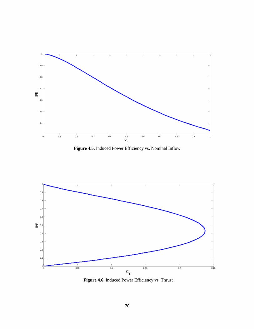
70

Figure 4.5. Induced Power Efficiency vs. Nominal Inflow

Figure 4.6. Induced Power Efficiency vs. Thrust

0 0.1 0.2 0.3 0.4 0.5 0.6 0.7 0.8 0.9 1

0.4

0.5

0.6

0.7

0.8

0.9

1

0

IPE

Figure 5. Induced-Power Efficiency versus Nominal Inflow

0 0.05 0.1 0.15 0.2 0.250

0.1

0.2

0.3

0.4

0.5

0.6

0.7

0.8

0.9

1

CT

IPE

Figure 6. Induced-Power Efficiency versus Thrust

71

Figure 4.7. Effect of Profile Drag on Induced Flow Efficiency

( ⁄

Figure 4.8. Effect of on Solidity in Hover

0 0.1 0.2 0.3 0.4 0.5 0.6 0.7 0.8 0.9 10

0.1

0.2

0.3

0.4

0.5

0.6

0.7

0.8

0.9

1

0

TR

E,

IPE

Figure 7. Effect of Profile Drag on Induced Flow Efficiency (Cd/C

l = 0.01)

IPE: Induced Power Efficiency

TRE: Total Rotor Efficiency Which Includes Drag (Figure of Merit)

0 0.1 0.2 0.3 0.4 0.5 0.6 0.7 0.8 0.9 10

1

2

3

4

5

6

0

,

'

Figure 8. Effect of 0 on Solidity in Hover

: Total Solidity

' : Projected Solidity

72

Figure 4.9. Optimum Twist Distribution for Ttpical Case

Figure 4.10. Optimum Chord Distribution for Typical Case

0 0.1 0.2 0.3 0.4 0.5 0.6 0.7 0.8 0.9 10

10

20

30

40

50

60

70

80

90

r

Figure 9. Optimum Twist Distribution for Typical Case ( 0 = 0.10)

0 0.1 0.2 0.3 0.4 0.5 0.6 0.7 0.8 0.9 10

0.1

0.2

0.3

0.4

0.5

0.6

0.7

r

(bc/

R),

(b

c/

R)

cos()

Figure 10. Optimum Chord Distribution for Typical Case

(bc/R)

(bc/R) cos()

73

Figure 4.11. Global Optimum Rotor in Hover

Figure 4.12. Universal Curve for Optimum Bound Circulation

0 0.002 0.004 0.006 0.008 0.01 0.012 0.014 0.016 0.018 0.020

0.02

0.04

0.06

0.08

0.1

0.12

0.14

Cd/C

l

0, C

T/

, C

T/

'

Figure 11. Global Optimum Rotor in Hover

0

CT/

CT/'

0 1 2 3 4 5 6 7 8 9 100

0.1

0.2

0.3

0.4

0.5

0.6

0.7

0.8

0.9

1

Figure 12. Universal Curve for Optimum Bound Circulation

74

Figure 4.13. Universal Curve for Wake Contraction Parameter in Hover

Figure 4.14. Velocities in the Far Wake

0 2 4 6 8 10 12 14 16 18 200

0.1

0.2

0.3

0.4

0.5

0.6

0.7

0.8

Figure 13. Universial Curve for Wake Contraction Parameter in Hover

0 0.5 1 1.5 2 2.5 3 3.5 40

1

2

3

4

5

6

7

8

Figure 14. Velocities in the Far Wake

75

Figure 4.15. Parameters in the Far Wake

Figure 16. Pressure in Far Wake for Global Optimum Rotor in Hover,

0 0.1 0.2 0.3 0.4 0.5 0.6 0.7 0.8 0.9 10

10

20

30

40

50

60

70

Figure 15. Pressures in the Far Wake

0 0.1 0.2 0.3 0.4 0.5 0.6 0.70

5

10

15

20

25

30

35

40

76

4.18. Appendix A: Summary of Formulas

The optimum induced-flow distribution and inflow angle at the blade are:

√

(

)

The thrust, induced power, and induced power efficiency (IPE) of this optimum rotor are

given by:

√

where is the swirl-loss function:

[

]

The optimum chord distribution for a given is:

(

) [

√ ]

and the total projected (i.e., weighted) solidity based on is:

(

)

[

] (

) [

]

The thrust and power coefficients––including the effect of profile drag are:

(

)

(

) (

)

77

where and are defined as:

(

) (

) (

)

(

)

(

)

(

)

The total rotor efficiency including profile drag is, therefore:

( √ )

4.19. Appendix B: Loading Integrals

The kernel of the loading integrals for thrust and power is given in Eq. (18) as:

∫ [

]

This can be rewritten in a form more conducive to integration

∫ [

]

This integrates directly into

[

]

which is equivalent to Eq. (19).

For the case of the ⁄ integral in the thrust equation, one must multiply the integrand of

Eq. (B1) by ⁄ . The resulting thrust is thus multiplied by with a

new integral defined as lacking one power of r, :

∫ [

]

78

Each term in Eq. (B4) can be integrated directly giving:

(

) (

) [ (

)

]

(

) (

) (

)

For the case of the power equation, one must multiply the integrand of Eq. (B1) by ⁄ . The resulting integral is similar to the power integral but multiplied by

⁄ ⁄ with an integral with an extra power of r, :

∫ [

]

The integrand of Eq. (B7) can also be rearranged for direct integration as follows:

∫ [

]

The integral follows directly as:

(

)

(

)

[ (

)

]

This can then be simplified to:

(

)

(

)

(

)

This completes the momentum integrals.

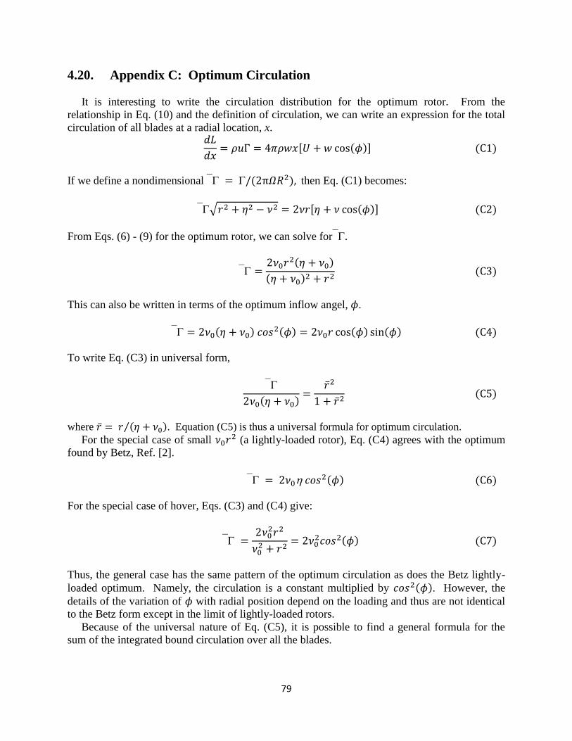
79

4.20. Appendix C: Optimum Circulation

It is interesting to write the circulation distribution for the optimum rotor. From the

relationship in Eq. (10) and the definition of circulation, we can write an expression for the total

circulation of all blades at a radial location, x.

If we define a nondimensional then Eq. (C1) becomes:

√

From Eqs. (6) - (9) for the optimum rotor, we can solve for.

This can also be written in terms of the optimum inflow angel, .

To write Eq. (C3) in universal form,

where ⁄ . Equation (C5) is thus a universal formula for optimum circulation.

For the special case of small (a lightly-loaded rotor), Eq. (C4) agrees with the optimum

found by Betz, Ref. [2].

For the special case of hover, Eqs. (C3) and (C4) give:

Thus, the general case has the same pattern of the optimum circulation as does the Betz lightly-

loaded optimum. Namely, the circulation is a constant multiplied by . However, the

details of the variation of with radial position depend on the loading and thus are not identical

to the Betz form except in the limit of lightly-loaded rotors.

Because of the universal nature of Eq. (C5), it is possible to find a general formula for the

sum of the integrated bound circulation over all the blades.

80

∫ [ (

)]

For large , this approaches ⁄ ⁄ .

4.21. Appendix D. Contraction Ratio

Background

In this Appendix, we derive the appropriate contraction ratio for a consistent momentum

theory. In Ref. [1] it is suggested that the contraction ratio should be such that the pressures in

the far wake balance the centrifugal forces on the rotating wake. However, Glauert is unable to

solve the equation for contraction ratio. A solution for this contraction ratio is attempted in Ref.

10], and a differential equation for the variable contraction ratio is obtained. However, on page

22 of Ref. [10] they write:

"In fact, it is shown in Appendix C that for 1 bounded and r(r1) a one to

one function, no solution of Eq. (38) exists which satisfies the boundary

conditions (39)." Ref. [10]

It is for this reason that they revert to the assumption of a constant contraction ratio that is

√ . The figure of merit from both Glauert and Ref. [10] are shown in the figure at the

end of this appendix, which is reproduced from Ref. [10].

On the other hand, there is a way to define the wake contraction function uniquely such that a

momentum theory remains consistent. In particular, the fundamental assumption for momentum

theory that leads to a consistent contraction ratio is:

The contraction ratio in the far wake for any annular ring must be such that the induced flow

at the rotor would cause a vortex sheet to come off of the rotor in a direction perpendicular to

the local lift with induced flow perpendicular to the sheet.

It is, of course, a premise of vortex theory that the sheet must be convected along the local free-

stream (which is affected by the induced flow) and that the lift on the blade is perpendicular to

the shed vortex sheet. For a momentum theory to be internally consistent, it must produce

induced flow perpendicular to this sheet.

Consistency Criterion

This criterion can be written in terms of the angles formed by the local flow velocities at the

rotor in hover. Namely, the angle of the lift (which is the angle of the induced flow) must be

along the same line as the induced flow.

⁄

81

This same fundamental equation appears in Ref. [1] as Eq. (4.6) on page 197. With this

assumption, one can see that either of Eqs. (54) – (56) immediately implies the other two. We

have shown in the body of the paper that the simplified contraction assumption––that the wake

expands to atmospheric pressure with a contraction ratio constant at √ and that the

unbalanced force from the momentum tube is included in the thrust balancemeets this

criterion; and this is why the unified momentum results derived herein are accurate.

Once Eq. (D1) is accepted, it is unnecessary to find the consistent contraction ratio explicitly.

Equation (D1) is sufficient in itself to derive the consistent thrust equations in Eqs. (54) - (56).

Nonetheless, the optimum contraction can be found––if desired––and it can then be used to study

the flow behavior in the far wake. This will be done in the paragraphs to follow.

For the more rigorous assumption that pressure remains in the wake such that it does not

expand to atmospheric pressure, the consistency criterion of Eq. (D1) can be expressed by

equating Eqs. (53) and (54).

[

(

) ] [

(

)

]

The correct contraction function is the one that makes Eq. (54) balance. If we assume that there

is some unknown mapping that takes a fluid particle from a point on the disk to a point

in the far wake by , we can write from geometry, continuity, and conservation of

angular momentum:

Placing Eq. (D3) into Eq. (D2) gives a determining equation in terms of and :

This can be solved by the quadratic formula for in terms of and .

√

82

Since it must be that maps into , the initial condition completes the

system.

Contraction for Betz Optimum

When the Betz inflow distribution from Eq. (6) is placed into Eq. (D5), the equation for

simplifies greatly. For example, simplifies to . The result is a universal differential

equation for the contraction mapping where ⁄ and .

√

As verification that this equation is the correct one for a consistent momentum theory, if one

takes Eq. (1.13) of Ref. [1], page 193 for the case of hover and substitutes into it the general

contraction mapping of Eq. (D3)––along with the Betz optimum solution––one obtains exactly

Eq. (D6) above. In the text just after Eq. (1.13) of Ref. 1, Glauert writes:

These equations, though rather complex in form, suffice to determine

the relationship between the thrust and torque of the propeller and the

flow in the slipstream. H. Glauert

Thus, one can say that the fundamental premise stated above––as to what constitutes a consistent

momentum theory––is consistent with the results of Glauert. Either approach results in the

identical equation for the optimum contraction ratio.

One can show that the solution to Eq. (D6)––and for the contraction ratio ––are, in the

limiting conditions:

(

)

(

)

[

]

√ [

]

Because the contraction ratio goes to zero near the root, it follows that the equivalent of vertical

vortex lines concentrate near the root. This implies that, in the far wake, both the axial and

circumferential components of normalized velocity converge to a finite value at the rotor center.

In particular, the limiting case is . This further implies that, near the

central axis, the wake rotation varies as ⁄ . In other words, the axial vortex lines near

the center are concentrated into a singularity, but it is not as strong as a pure, concentrated vortex

with ⁄ which would give infinite circumferential velocity. Interestingly, this implies

that the correct contraction ratio gives an unbounded value for 1 which explains why Ref. [10]

could prove that no solution exists for "bounded ." In fact, the correct solution is unbounded

at the root due to the concentration of vorticity.

Equation (D6) can be solved numerically because the solution in Eq. (D7) can be used to

circumvent the singularity at . To be specific, one integrates from a small (for which

83

is known) out to , the latter of which maps the location of the outside of the far

wake. Figure 13 shows the resulting universal contraction ratio as a function of . For

small , the contraction is slightly less than √ except near the root where it goes to 0. This

is in agreement with the statements made about contraction ratio in Ref. [10]. For practical

purposes, a good approximation to the contraction ratio over the entire range of values is:

which can be used in numerical work. matches the first term of the small- expansion and the

first two terms of the large- expansion exactly. Thus, there is only one free parameter used in

obtaining this good fit. Figure 13 shows both and the approximation plotted on the same

curve, and they are virtually identical.

Conditions in the Far Wake

It is interesting to look at the solution for the velocities and pressures in the far wake under

the assumption of a consistent contraction ratio. Figure 14 shows the axial velocity and the

circumferential velocity as functions of the local normalized radius . This is a universal

curve for any rotor radius . Thus, the location of the blade tip is:

√ (

)

Although the velocities at the central axis are zero at the rotor disk, the axial vortex lines

concentrate into a singularity at the rotor center (as the flow travels downstream); and this results

in finite velocities at the center in the far wake.

From these, it is possible to determine the pressure in the downstream wake from Eq. (51):

(

)

Since the wake contraction parameter is written in terms of the normalized radius on the rotor

disk, it is convenient to write both the radius in the far wake––Eq. (D9)––and the pressure in the

far wake––Eq. (D10)––in terms of the generating radius at the rotor disk:

[

] ⁄

where we have used the Betz optimum for the velocities. However, since is given by the

differential equation in Eq. (D6), the above can simplified to:

[

] ⁄

84

This is a negative pressure in the far wake and is shown in Fig. 15 as a function of . Note that

the normalized pressure at the central axis of the far wake is 64. This is consistent with the

velocities at the center, since PW = (82 + 8

2)/2 = 64.

It is interesting to compare this pressure with the pressure that would be required to hold the

centrifugal force of the Betz distribution in equilibrium. We normalize on the quantity

as in Eq. (D10).

∫

∫

⁄ ⁄

where the integrand and limits can be written in terms or by use of Eq. (D3). This integral can

be done numerically and is shown in Fig. 15 as a universal curve. To exactly match the

boundary condition at the tip, simply translate by the value of at the tip, ⁄ ⁄ as indicated by Eq. (D13).

One can see that, although from momentum theory does not exactly match the pressure

necessary to balance centrifugal forces in the far wake ( ), is qualitatively accurate. The

differences between the two are interesting. While goes to infinity at the central axis (a

logarithmic singularity), remains at a finite (although very large) value. Both distributions

decay with and cross at the point . They both continue to decay as radius

increases. Thus, is higher at small radii; while is higher at larger radii. While is to be

translated down by ( ) in order to match the boundary condition outside of the wake,

is independent of rotor radius such that there is always a residual pressure at the wake boundary

that must be reacted by the momentum tube––in keeping with the assumptions of momentum

theory.

The fact that the momentum theory result cannot exactly match the centrifugal pressure was

rigorously proved in Ref. [11]. That paper shows that the equations of momentum theory imply

that the flow in the annular momentum tubes cannot remain in segregated tubes and yet satisfy

all of the dynamic conditions of the flow. The true solution will involve mixing among the

annular tubes. This implies some further losses not predictable by momentum theory. In short,

momentum theory is not an exact solution to the potential flow equations; and, therefore––while

it can balance forces, moments, momentum, and angular momentum––it cannot meet all

equilibrium conditions of the flow. Nonetheless, consistent momentum theory is a good

approximation and represents an important upper bound on lifting rotor efficiency.

85

Figure 9 of Ref. [10] where , , and REF. 5 is Glauert.

ideal optimum performance of propellers, lifting rotors

Documents