icpms standard operating procedures-liquids contents · the argon plasma is capable of breaking...

i

ICPMS Standard Operating Procedures-Liquids

Contents Introduction ................................................................................................................................................. iii

Instrument Hazards and Best Practices: ICP-MS .......................................................................................... iv

1. Concise Operating Procedures .................................................................................................................. 1

2. ICP-MS Theory and Operation .................................................................................................................. 2

2.1. Instrument Operation ........................................................................................................................ 2

2.1.1. Plasma ......................................................................................................................................... 2

2.1.2. Interferences ............................................................................................................................... 2

2.1.1. Cones ........................................................................................................................................... 2

2.1.2. Lenses .......................................................................................................................................... 2

2.1.3. Octopole Reaction System .......................................................................................................... 3

2.2. Sample and Standard Preparation ..................................................................................................... 4

2.2.1. Liquids ......................................................................................................................................... 4

3. Hardware Setup ........................................................................................................................................ 6

3.1. Current Setup ..................................................................................................................................... 6

3.2. Laser Ablation to Liquids .................................................................................................................... 7

4. Igniting the Plasma .................................................................................................................................... 9

4.1. Turn on the Water Chiller .................................................................................................................. 9

4.2. Turn on the Argon .............................................................................................................................. 9

4.2.1. Liquid Argon Tank Operation ....................................................... Error! Bookmark not defined.

4.3. Ignite the Plasma.............................................................................................................................. 10

5. Analyzing a Liquid Sample ....................................................................................................................... 12

5.1. Setting up the Hardware (autosampler and peripump) .................................................................. 12

5.1.1. Peristaltic Pump Setup .............................................................................................................. 12

5.1.2. Autosampler Setup ................................................................................................................... 13

5.1.3. Internal Standard Tubing Setup ................................................................................................ 15

5.2. Analyzing Your Sample with a Sequence ......................................................................................... 16

5.2.1. Throwaway Samples ................................................................................................................. 17

6. General Software Overview .................................................................................................................... 18

6.1. Before Starting the Software ........................................................................................................... 18

6.2. Layout ............................................................................................................................................... 19

AMSEC rev. 01/2019 KTM Back to Concise Procedures ii

6.3. Instrument Control .......................................................................................................................... 20

6.4. Tuning Panel ..................................................................................................................................... 22

7. Creating/Editing a Method ..................................................................................................................... 23

7.1. Method Information ........................................................................................................................ 24

7.2. Select Sample Types ......................................................................................................................... 25

7.3. Interference Equations .................................................................................................................... 26

7.4. Acquisition ....................................................................................................................................... 27

7.4.1. Spectrum ................................................................................................................................... 27

7.4.2. Time Resolved Analysis ............................................................................................................. 31

7.4.3. Spectrum (Multi Tune) .............................................................................................................. 35

7.5. Peristaltic Pump Program (Liquids only) .......................................................................................... 39

7.6. Saving a Method .............................................................................................................................. 40

8. Sequence Files: Creating/Editing for the Autosampler (Liquids only) .................................................... 41

8.1. Method Column ............................................................................................................................... 43

8.2. Type Column .................................................................................................................................... 43

8.3. Vial Column ...................................................................................................................................... 44

8.4. Data File Column .............................................................................................................................. 44

8.5. Sample Column ................................................................................................................................ 45

8.6. Dil/Lvl Column .................................................................................................................................. 45

8.7. ISTD Conc Column ............................................................................................................................ 45

8.8. Helpful Hints .................................................................................................................................... 45

8.9. IMPORTANT: Throwaway Samples .................................................................................................. 46

8.10. Reanalyzing a Sample Midrun ........................................................................................................ 47

9. Data Analysis Window ............................................................................................................................ 48

9.1. Software Overview ........................................................................................................................... 48

9.2. Batch Files (Liquids).......................................................................................................................... 49

9.2.1. Creating a Batch File ................................................................................................................. 49

9.2.1 Looking at Data and Calibration Curves ..................................................................................... 54

9.3. Exporting and Viewing Data (Liquids) .............................................................................................. 56

9.3.1. Average CPS View ..................................................................................................................... 56

9.3.2. Concentration View .................................................................................................................. 56

9.3.3. Total Replicate View.................................................................................................................. 57

9.3.4. Exporting Data........................................................................................................................... 58

AMSEC rev. 01/2019 KTM Back to Concise Procedures iii

9.4. Batch Files (Laser Ablation) .............................................................................................................. 59

9.4.1. Creating a Batch File (Time Resolved Analysis) ......................................................................... 59

9.4.2. Creating a Batch File (Spectrum)............................................................................................... 61

9.5. Exporting and Viewing Data (Laser Ablation) .................................................................................. 63

9.5.1. Time Resolved Analysis ............................................................................................................. 63

9.5.2. Spectrum Analysis ..................................................................................................................... 65

10. Tuning the Instrument .......................................................................................................................... 66

10.1. Selecting a Tune File ...................................................................................................................... 66

10.2. P/A Factor Tuning (Liquids) ............................................................................................................ 67

11. Preferred Isotopes and Interferences ................................................................................................... 68

12. Shutting Down the Instrument ............................................................................................................. 70

12.1. Shutting Down with Liquids ........................................................................................................... 70

12.2. Shutting Down with Laser Ablation ............................................................................................... 70

13. Troubleshooting and Error Help ........................................................................................................... 71

13.1. Plasma Ignition ............................................................................................................................... 71

13.2. Pumping Issues (Liquids Only) ....................................................................................................... 72

13.3. Issues with Batch Files ................................................................................................................... 72

13.4. Data not Displaying at all in the Data Analysis Window ................................................................ 73

13.5. Issues with Noisy Data and High Backgrounds .............................................................................. 73

Introduction This manual is made to be a comprehensive refresher for people who have previously been trained to use the instrument. It is divided into individual sections which are often interrelated and may not be next to each other. Refer to the concise operating procedures for either liquids or laser ablation. In the concise procedures, references will be given to in-depth instructions located in the document in case you need more information. In case there are issues, see Section 14. Troubleshooting and Error Help. Make sure you contact the lab manager with any issues or trouble you are having. Kyle Mikkelsen The local login for the computer is Lab Manager required due to proper instrument [email protected] file permissions. It is as follows: Tel: (360) 650-4280 Login: .\AMSEC Password: AMSEC See the sign outside the office door for Kyle’s current location. ES 130 (down the hall from the lab) Juliet (ES 131) can always contact me if I am in the office. Use the messaging app as well to contact Kyle in case of questions.

AMSEC rev. 01/2019 KTM Back to Concise Procedures iv

Instrument Hazards and Best Practices: ICP-MS This document will cover the inherent hazards when utilizing this piece of equipment as well as the best practices and procedures to avoid danger. These hazards will not include basic things that may be included in the basic safety training document that each user has attested to have reviewed at fom.wwu.edu/documents. Lab coats are to be provided by the user unless special hazards exist in which case they are located at the PPE station. Hazards:

- Chemical exposure - Compressed gases - Ultraviolet light exposure - Ultraviolet laser radiation

1. Required PPE Appropriate laboratory attire is required at all times in the AMSEC laboratories. Whenever chemicals are being used, an additional requirement of a lab coat is required. Lab coats are to be provided by the user.

Whenever a user is in the AMSEC labs, the minimum requirement for eye protection is wrap around impact glasses. Anytime liquid chemicals are present in the same room as the user without a direct barrier, all users in the lab must wear chemical splash goggles. Splash goggles must be approved by State of Washington Administrative Code (WAC 296-24-078).

If chemicals being used are considered toxic, caustic, corrosive, flammable solvents, carcinogenic, mutagenic, or teratogenic, a minimum of disposable nitrile gloves is required. Avoid chemical transfer by taking off gloves when using anything other than the chemical(s). 2. Compressed gases All users must have completed the compressed gas and cryogenic liquid training before accessing this equipment or touching any compressed gas cylinder or cryogenic liquid tank. All prudent practices dictated in that training as well as associated training documents must be strictly adhered to at all times. 3. Ultraviolet light exposure

The argon plasma associated with this instrument emits harmful levels and wavelengths of ultraviolet radiation that is harmful to the eyes. Every effort is taken to reduce the risk of ultraviolet light exposure, however it is impossible to eliminate all possibilities, especially when an accessory item such as the laser ablation is being used which isn’t designed with that in mind.

It is recommended to avoid eye contact with the plasma at all times unless using the properly shielded window located on the front of the instrument. Placing the protective orange plastic over the hole where the sample is introduced is also recommended to reduce the possibility of making eye contact. 4. Ultraviolet laser radiation The ICP-MS is equipped with a laser ablation accessory system. It utilizes a high powered, 213 nm laser to ablate samples. This laser system is designed with many interlocks and safety devices in place to prevent users from ever being exposed to the laser. Under normal operation, the chances of being exposed to the laser are almost zero. If any interlocks are not satisfied and cannot be remedied by the user, the lab manager must be notified and the user should cease use of the system immediately.

At no time should anyone tamper with or attempt to dismantle or repair any part of the instrument. Failure to follow these instructions could lead to serious injury or death.

http://fom.wwu.edu/fom/documents

AMSEC rev. 01/2019 KTM Back to Concise Procedures 1

1. Concise Operating Procedures The concise operating procedures outline the necessary steps and reference relevant sections for more detailed instructions. Steps 2-4 can be done in any order. 1. Check the hardware setup and change to

liquids if necessary. 2. Setup the peristaltic pump and the

autosampler. 3. Open Software and ignite the plasma.

(Check Configuration Beforehand) 4. Load your samples and standards while it

lights. 5. Open the three rinse bottles. 6. If the ICP-MS was run with Laser Ablation

before you, perform a P/A Factor tune. (don’t forget to put the ISTD tube in the nitric and back to the ISTD bottle after the P/A tune)

7. Load your tune file. Rinse the probe. 8. Load your method file. Edit as required.

Choose Method Load 9. Setup your sequence file. 10. Create your batch file. 11. Run your standards and samples.

12. Check your calibration curves. Edit as

necessary. 13. Export your data. 14. Turn off the instrument.

a. Shut off plasma if not already off b. Release the peripump tubing and place

the ISTD in the nitric bottle. c. Send the autosampler probe home. d. Release the autosampler peripump

clamp and shut it off. e. Shut off the argon and water chiller.

16. Take your samples and clean up.

Section 3. Hardware Setup Section 5.1. Setting up the Hardware Section 4. Igniting the Plasma Section 6.1. Before Starting the Software Section 5.1.2. Autosampler Setup and Section 8.3. Vial Column Section 10.2. P/A Factor Tuning Section 10.1. Selecting a Tune File Section 7. Creating/Editing a Method Section 8. Sequence Files: Creating/Editing Section 9.2.1 Creating a Batch File Section 5.2. Analyzing your Sample with a Sequence Section 9.2.1 Looking at Data and Calibration Curves Section 9.3. Exporting and Viewing Data Section 12.2. Shutting Down with Liquids


2. ICP-MS Theory and Operation 2.1. Instrument Operation 2.1.1. Plasma Inductively coupled plasma-mass spectrometry (ICP-MS) is a technique that utilizes an extremely hot argon plasma of ~10,000 K for the purpose of atomizing/ionizing any sample for trace elemental analysis. The sample introduction method for this system is either a liquid autosampler capable of continuously running up to 200 samples or a laser ablation system which utilizes a 213 nm high powered laser to ablate a solid sample which a helium flow then takes to the plasma. Regardless of the sample introduction method, the operation of the instrument itself follows the sample principles.

The argon plasma is capable of breaking apart any molecule into atoms while simultaneously ionizing these atoms. Ionized atoms and molecules interact with magnetic fields due to an induced dipole from the loss of an electron, but we only want to measure atoms and not molecules. Therefore, a series of electromagnetic lenses have been devised to focus the ion beam and remove any polyatomics that may have been formed by the plasma or recombined after going through the plasma. 2.1.2. Interferences The large majority of the ICP-MS system is dedicated to removing interferences. What exactly are interferences? This term refers to anything that can interfere with the analyte mass in question. The masses are measured at the end of the instrument by an ion counter. This counter doesn’t know what is hitting it, it just counts the ions that hit. The quadrupole located directly before the ion counter is what filters out every ion except the one to be measured, and it is here that the effects of interferences are seen, but you don’t know it. The quadrupole filters things by their mass to charge ratio. This means that if you are analyzing an ion of iron such as 56Fe+ then the mass to charge ratio is 56/+1. There are other things that can result in the same mass to charge ratio such as argon oxide, 40Ar16O+. This will have the same mass to charge ratio and every one that makes it to the quadrupole will be detected as if it were 56Fe. 2.1.1. Cones

Upon going through the plasma, a portion of the sample is single, ionized atoms, a portion is ionized molecules, and a portion is neutral atoms and molecules. The first thing the sample stream comes into contact with is a set of nickel cones. The first cone is called the sample cone which is aligned such that only the hottest part of the plasma is sending sample into the lens chamber. This is beneficial since the hottest part has the highest amount of ionized atoms. The second cone known as the skimmer cone, has a smaller orifice which skims off even more of the stream that wasn’t going in a straight line and reduces the sample stream to a smaller, more manageable size. Between the plasma chamber and the lens chamber, the pressure goes from atmospheric to a rough vacuum of ~10-3 torr. This helps suck in the sample stream and allows for less collisions with gas molecules to increase the mean free path of the sample stream. 2.1.2. Lenses

After going through the set of cones, the sample stream is subjected to a set of electromagnetic lenses which focus the ion beam while allowing a large portion of neutrals to be sucked away by the vacuum. The next set of lenses deflects the ion beam by a couple millimeters. This is a key feature of the lens set since any neutral atoms/molecules that have made it this far will continue to fly straight and are ran into a plate and subsequently sucked into vacuum. The other reason for this deflection is to also remove any direct path for photons generated by the plasma to hit the electron multiplier tube at the end of the instrument as this


would damage it. Up to this point so far, we have atomized and ionized a sample and refined and focused the beam into ionized atoms and ionized molecules. 2.1.3. Octopole Reaction System

The rest of the analyzer chamber is at a vacuum of around 10-6 torr and the ion stream is pulled into the octopole reaction system (ORS). This is a specially designed cell with a set of eight small rods arranged in a cylinder shape. The rods have an electromagnetic field applied to keep the ion beam focused and flying straight. Just before entering the cell, the ion beam passes through an entrance pinhole which has a potential applied to it. Any ionized particle that doesn’t have enough momentum cannot make it over this potential barrier is removed from the stream. Once the ion beam enters the ORS, there is one of three configurations that can be used.

The first is known as nogas mode. In this mode the ORS is under vacuum and simply focuses the beam to send it into the quadrupole mass analyzer. The second mode is helium mode. In this mode, also known as collision mode, the ORS is filled with helium gas. Statistically, larger ions, such as polyatomics, will collide with the helium much more frequently than the much smaller atoms that are passing through. This will either cause them to be ejected from the cell and sucked into a vacuum pump, or it will cause them to lose so much momentum that they will be unable to overcome the cell exit potential barrier. This mode is the most effective at removing polyatomic interferences.

The third mode is hydrogen mode, also known as reaction mode. Similar to helium mode, in hydrogen mode the cell is filled with hydrogen gas. Also similar to helium mode, collisions take place that remove polyatomics. The difference lies in the fact that the hydrogen can easily react with any ion and form a neutral molecule or a polyatomic with 1 amu added to the mass. Upon collision and reaction, the now neutral molecule will have changed course since it will not interact with the field generated by the octopole and will be sucked into a vacuum pump instead of heading into the quadrupole. Hydrogen mode and helium mode are often used for only very specific atoms which have specific interferences. Both of these modes severely lower the overall counts of everything due to collisions and reactions taking place with both atomic and polyatomic ions in the stream, but the interferences are reduced much more than the atomic ions.

The sample stream has now been refined to a very uniform ion beam of only single atoms. This beam now enters the quadrupole mass analyzer which is capable of utilizing strong electromagnetic fields to “filter” out every isotope that is not of interest. The quadrupole will scan across the entire range of masses selected by the user to give the mass spectrum of interest. The integration time as selected by the user, dictates how long signal is collected for each isotope. Once the isotope of interest is selectively chosen by the quadrupole, it then makes its way to the end of the instrument to the electron multiplier (EM). In the EM, every atom that hits the detector plate ejects some electrons, which then cascade into another plate, multiplying the signal by several orders of magnitude until they are finally read at the end as a current. This current is proportional to the number of ions detected and results in the counts that are seen on the screen.


2.2. Sample and Standard Preparation Samples for ICP-MS must be kept as clean as possible. Things such as skin oils, dust, contamination from unclean sample holders, and contamination from user error are all things that contribute significantly to the error of the measurements obtained with this instrument. Proper analytical techniques must be applied to ensure the cleanliness and reproducibility of your measurements. 2.2.1. Liquids For liquid samples, many different types of things can be analyzed. Commonly done are water samples, digested plant and soil samples, and dissolved solid samples. An important characteristic of liquid samples is that they must be free from particulates. Any particulate over 0.50 µm can clog the sample line causing potential hours or days of instrument downtime. It is recommended that you filter every sample if this is a concern. The other option is to centrifuge samples directly prior to analyzing to settle any particulates to the bottom of the sample tube. A common term that is used when referring to liquid samples and standards is “matrix”. It is often commented that the sample and standard matrix must be the same. This is referring to the environment of the samples. The matrix is often the acid used to dissolve the samples which is required even in water samples to help dissociate any metal complexes that may have formed naturally. This means that the acid concentration of the samples and the standards must match exactly. When the sample is introduced into the plasma, it must behave the exact same way as the standards do, otherwise the data will not be quantifiable. The ICP-MS tubing we have can only handle up to 5% acid content and cannot be used with hydrofluoric (HF) acid. Commonly used acids are nitric (HNO3) and hydrochloric (HCl). When using hydrochloric acid, interferences are greatly increased and the ORS must be used in either helium or hydrogen mode. Sulfuric acid (H2SO4) can also be used, but is not recommended due to the diprotic nature and addition of excess sulfur. A common concentration of acid is 2% and is highly recommended. When preparing the standards for your samples, match the matrix to that of the samples themselves. The standards must contain any elements that you wish to quantify with the ICP-MS since you are creating calibration curves for each. The standards should encompass the range of suspected sample concentrations you expect. This means that you must have a

9

1) Argon Plasma 2) Sample Cone 3) Skimmer Cone 4) Lens Stack 5) Octopole Rxn Cell 6) Quadrupole Mass Analyzer 7) Electron Multiplier 8) Turbomolecular Pump 9) Roughing Pump

1 2 3 4 5 6 7

8


standard concentration that is higher and lower than your sample’s concentration. A typical set of standards will start at 100 ppm (mg/L) and go down by dilutions of ten to 1 ppt (ng/L), although sometimes they can go slightly higher to 1 ppT (g/L), but usually don’t go lower than 1 ppt. An example is 100 ppm, 10 ppm, 1 ppm, 100 ppb (µg/L), 10 ppb, 1 ppb, 100 ppt, 10 ppt, 1 ppt. The standards should be made with ultrapure water and trace metals acid and should include a blank of the same ultrapure water and acid of the same concentration. The blank is necessary and is used to calculate detection limits. Sample preparation is very important, but is highly specialized to each user and their sample type. Therefore, sample prep should be discussed with your research advisor or the lab manager prior to attempting ICP-MS.


3. Hardware Setup 3.1. Current Setup There are two possible setups for the ICP-MS. One is for laser ablation and the other is for liquids. The following two pictures display: Laser Ablation (left) and Liquids (right)

• The instructions for changing from laser ablation to liquids are on the following pages.


3.2. Laser Ablation to Liquids 1) To change from the laser ablation setup to liquids you must first open the torch-box

cover and disconnect the sample line ball joint by removing the spring clamp as seen:

2) Then disconnect the carrier gas line from the tube going to the laser ablation accessory:

3) 4) Insert the spray chamber making sure the ball joint and the drain connection seat

properly and connect the carrier gas line using the ez-lock fitting. Instructions should be posted on the instrument. Simply push the tubing into the yellow connector.

Ball Joint

Spray Chamber Seat

Carrier Gas Line

EZ-Lock


5) 4Place the spring clamp on the ball joint and then place the insulating cover on the spray chamber and tighten the knurled white knobs. Tighten these so they are snug but do not overtighten as the threads can be easily stripped. Close the cover over the torch box.

• The ICP-MS is now ready for use with liquids!

Knurled Knobs


4. Igniting the Plasma 4.1. Turn on the Water Chiller • The water chiller is located in ES 128B. This is the small room just adjacent to the ICP-MS

room. The chiller should turn on around room temperature and then cool to ~20°C.

• You must turn on the water chiller before lighting the plasma. If you forget, it will not damage

the instrument, but you will receive an insufficient water flow error.

4.2. Turn on the Argon Argon Manifold Operation

To operate:

1. Open both argon tanks. Check pressure in each. 2. If one tank is below 250 psi, change according to procedure below. 3. Check that output pressure is between 50 and 100 psi. Adjust as necessary.

When finished: 1. Change tank(s),

if required. 2. Close both argon

tank valves.

Argon tanks

Purge valves

Tank pressure

Output pressure

Output pressure adjustment

Primary tank selector


To change a tank: 1. If a tank has dropped below 250 psi, it can be changed whether the argon is being used

or not. 2. Turn arrow knob toward the tank with more argon. 3. Close tank valve of empty tank. 4. Disconnect nearly empty tank, cap it, and replace with a full one. 5. Strap full tank in, remove cap, and attach pigtail hose. 6. Open tank valve for the tank you just attached. 7. Slowly open purge valve for the tank you just attached and purge for 5 seconds. You do

not have to purge at a high flow rate, just enough to get any air out of the system. This system is designed to offer continuous, uninterrupted gas delivery. You can change a

tank while the system is being used. The arrow knob indicates the primary tank. The primary tank will be used until it is around 200 psi, this will be considered empty. The system will then switch to the secondary tank.

You must check the pressure in each tank multiple times during a run. If you empty a tank, you must change it. Do not leave it for the next person to change.

4.3. Ignite the Plasma • After the water chiller and argon tank has been turned on. You must make sure that your

sample introduction is set to the desired configuration before lighting the plasma. See Section 3. Hardware Setup for more information.

• Go to the instrument control panel in ICP-MS Top and click Plasma On in the plasma menu or hit the Ignite Plasma icon.

• You will be prompted with two dialogue boxes. The first will ask if the exhaust system is working. Click yes.

• The second will ask to verify that the drain tubing is connected. Since you are using liquids, you must do this before starting the plasma. See Section 3.1. Setting up the Hardware for more information. Once the tubing is connected properly, click yes on the dialogue.

• The plasma should light after a few minutes. The status bar of the instrument control window

will show standby --> analysis until it is ready for operation. Once it is ready for use the

Drain Tube

To Waste


status bar will only say analysis mode. See the Section 6.3. Instrument Control for more information.

Left: Instrument control window in analysis mode without a reaction gas. Right: Instrument control window in analysis mode with a reaction gas.


5. Analyzing a Liquid Sample This section will cover how to analyze a liquid sample. We will only use the autosampler as the manual sampling method incurs too much human error and contaminates the system easily.

5.1. Setting up the Hardware (autosampler and peripump) • First, see Section 3. Hardware Setup to determine if you need to switch from the laser

ablation setup to the liquids setup and change if necessary. 5.1.1. Peristaltic Pump Setup • Stretch the tubing for the peristaltic pump such that the tabs hook into the notches. It is

important to trace the direction the liquids will be pumped based on the arrows on the side of the pump. The order from left to right for the tubes must be: Sample, ISTD, and Drain.

• Note the elasticity of the peristaltic pump tubing along with the cleanliness. If it is stretched

out and doesn’t require any effort to pull over the notches, consider using the secondary segment for pumping (each tube has two sections which can be stretched for pumping).

• Next, close the black clamping mounts by clamping the spring-loaded rod down as seen:

• Double check the flow of the fluids. The sample line should come from the autosampler and

go into the bottom of the pump and from the top go to the ISTD mixer (white tee shaped device on the back of the pump seen in red above right). The ISTD tube should come from one of the poly bottles nearby and go into the bottom of the pump and from the top go to the ISTD mixer. The drain tubing should go from the bottom of the spray chamber into the bottom of the pump and from the top go into a waste bottle nearby. The line from the top of

Drain ISTD Sample

ISTD Mixer

Liquid Flow

Adjustment Knobs


the ISTD mixer should go to the nebulizer. NOTE: Make sure to never turn the adjustment knobs on the clamps. This will change the very delicate pressure applied to the tubing which will mess up all the fluid flow.

5.1.2. Autosampler Setup • Turn on the autosampler and hook up the peripump on the back. This is a view from the

backside with the power button on the left (confirmed by a green light on the front) and the peripump is on the right.

• The peristaltic pump on the back should never have the tension released on the tubing.

Simply fold the clamp over and latch it with the spring-loaded rod (inset photo). • The large bottle in the middle is nanopure water and should be replaced before every run.

Be careful to keep the tube that goes into it clean. Empty the bottle and follow the instructions on the nanopure system by the sink to refill. The kimwipe is to keep dust out. Never set the tubing on the table. Always set it on a clean, large kimwipe.

IMPORTANT: You will need to verify that the pump is actually working. Sometimes it doesn’t pump right away and you have to help it. To do this, make sure the autosampler is set up and you have gotten the software configured properly. Then tell the ALS to rinse from either the tune panel or the instrument control panel. After it starts to rinse, watch the tubes in the back to ensure that water is flowing. If it isn’t flowing, pinch the clamp as shown to the right. The water should start to flow after that.


• Next, load up your standards and samples. Standards should be loaded from least

concentrated to most concentrated. For more information on sample positioning see Section 8.3. Vial Column for more information.

Least Conc.

Most Conc.


5.1.3. Internal Standard Tubing Setup • It is very important to perform the next step as your quantification relies on it. The ISTD tube

must be switched between one of two bottles depending on what operation you are performing. The 2% nitric bottle is for storage and tuning the instrument. The ISTD bottle is for running samples and standards.

• To switch the tube between the bottles, unscrew the cap of the bottle the tube is to be

placed in next and place it face down next to it. Then unscrew the cap of the bottle with the tube in it and pull out the cap and tube together. Take a clean kimwipe and wipe the tube off. Take care to never touch the tube to anything else as it will contaminate it. Place the tube into the new bottle to be used and screw on the cap. Take the leftover cap and place it on the bottle the tube just came out of. (There is only one cap with a hole for the tube)


5.2. Analyzing Your Sample with a Sequence You must have a method created before setting up or running a sequence file. For information on this, see Section 7. Creating/Editing a Method. You should have ignited the plasma and selected your tune file also, but you can set up sequences in advance. See Section 1. Concise Operating Procedures for Liquids for more information. • Set up your sequence file as described in Section

8. Sequence Files. • Once your sequence file is set up and saved, you

are ready to begin a sequence. • From the Sequence dropdown, select Run. • The Start Sequence Dialogue will appear.

• Unless you are confident that you want to, do not check the Overwrite Existing Data Files

box. This will overwrite any file with the same name. • Next, use the Browse button to locate your batch file. For more information on this, see

Section 9.2. Creating a Batch File. Copy the file address just in case. This usually comes in handy.

• Click Run Sequence and the autosampler will begin. • If the Data Analysis window is not already open, it will open and the data will appear there.

For more information see Section 9.2. on Creating a Batch File.


5.2.1. Throwaway Samples IMPORTANT: We have been having troubles with the autosampler communicating properly with the computer, but we have figured out a workaround. Hopefully this can be fixed in the near future. For now, see Section 8.9. Throwaway Samples. Notes: • Make sure that the rinse vials you have selected are open and filled properly. This is

selected in your method. See Section 7.5. Peristaltic Pump Program for more information. • Make sure that the ISTD tube is in the ISTD bottle. • Make sure the autosampler peristaltic pump is clamped for operation and the large

nanopure bottle is filled with fresh water.


6. General Software Overview 6.1. Before Starting the Software • Before the ICP-MS software can be opened, the configuration must be set properly based

on which mode, Liquids or Laser Ablation, the instrument will be run in. • First, click on the Configuration icon on the desktop. This must be done

with the ICP-MS Top window closed along with any other masshunter windows.

• Once the window opens, ensure that it looks as seen below for either Liquids (Top) or Laser

Ablation (Bottom), then click save and proceed to open the ICP-MS Top software:

Liquids

Laser Ablation


6.2. Layout • Upon opening the software by clicking on the desktop, the general layout for the

software will look like this:

• Most of the important menus and information are in the top left:

From left to right across the menu bar:

1) Instrument: enter the instrument control and tune panel 2) Acquire data: perform a measurement manually 3) Data analysis: opens the Masshunter online data analysis window for data handling 4) Methods: load, save, edit, and run a method 5) Sequence: load, save, edit, and run a sequence 6) The rest are not typically used

From left to right across the icon bar: 1) Instrument Control 2) Tune Panel 3) Acquire Data 4) The rest are not typically used

From left to right below the icon bar: 1) Method: Displays the currently selected method. The most recently used 4 are in the

dropdown. 2) Sequence: Displays the currently selected sequence file. (LA users don’t use a

sequence file)


6.3. Instrument Control • To enter instrument control, go through the instrument menu on the menu bar or click the

left-most icon:

• When the plasma is not lit, the control window will look like this:

From the instrument control window, we have the following:

1) The plasma menu where you can ignite or shut off the plasma 2) The plasma ignite icon 3) The plasma shut-off icon 4) The gas flow meters 5) The analyzer (left) and backing (right) pressure gauges 6) The RF generator meters (left) and the water flow meter (right) 7) The spray chamber temperature gauge

Notes: -to view a meter value, click and hold the meter icon on the diagram. -the title bar says that the instrument is currently in standby mode. This will indicate the current status of the instrument. -to light the plasma, see Section 4. Igniting the Plasma.


• When the plasma is lit, the instrument control window will look one of two ways. If there is no reaction or collision gas, it will look as follows:

• If there is a reaction or collision gas being used, then the window will look as follows:

Notes: -On both windows, the title bar says it is in analysis mode. You must wait for it to say this during ignition before you will be able to access the tuning panel. You can also access the tuning panel while in standby mode. -The instrument status may show it is standard or reaction mode upon ignition regardless of what mode the user intends to run in. This is due to the mode the last user ran the instrument in. As long as the correct tuning file is chosen before or after ignition, the instrument will operate in the correct mode. See Section 10.1. Selecting a Tune File for more information.


6.4. Tuning Panel • To enter the tune panel, go through the instrument menu on the menu bar or click the

second from the left-most icon:

• The tuning window is shown below:

The menu bar of the tune window has the following options the user can access:

1) File-load and save a desired tune file 2) Tune-perform autotune and P/A Factor tuning. 3) Acq. Params-change which masses are being monitored in a sensitivity tune 4) ALS-control the autosampler (liquids) 5) The rest are not typically used.

• The Tune File box below the menu icons shows the current tune parameter file. • The white area on the left displays the current instrument parameters. • The area to the right of the tune parameters is the sensitivity tuning section. We generally do not allow student users to tune the instrument. This is for informational purposes only. Notes: - The autune.u file is loaded by default. This file is the one that the instrument reads to run an experiment. The file parameters are equivalent to the parameters the user had loaded when the tune panel was closed last.


7. Creating/Editing a Method The creation of the method file is perhaps the most important part of the analysis using ICP-MS after proper sample preparation. The method file is what tells the mass spectrometer what to measure, and it will only measure what is in the method file. In the case of sparsely available or tough to prepare samples, an error in the method could mean disaster if an isotope wasn’t measured that needed to be. Take care when making a method and always double check everything! • To edit a method, you must choose a method similar to yours to edit, or start with the

DEFAULT.M method. To do this, select “load” from the method dropdown menu. Note: It is not recommended that you edit someone else’s method without their permission as it is easy to overwrite their configuration. • Start by selecting “edit entire method” from the method dropdown menu. See Software

Layout for more information. The following box should appear:

• We will go through all four of the options to see what the dialogue looks like. In the future, if

you are editing your own method, you can select only the options you would like to edit. • Select OK to move on to Method Information


7.1. Method Information

• The comment section of the Method Information dialogue can be read when you are loading

a method and is useful for ensuring you are using the correct method. • The two check boxes selected are optional.

o By saving a copy of the method with the data, you will have a snapshot of your method file in case you change it in the future and don’t remember what configuration was used while collecting past data.

o The option to tabulate chart to CSV is only for users running in timechart mode, also called time resolved analysis. This will automatically tabulate all your data in either CPS (counts per second) or in the raw format. If you are unsure of the difference contact the lab manager for more information.

Note: There have been some issues with checking the “Save Copy of Method With Data” checkbox when sampling with a sequence file. The user receives “sequence error or user terminated” error. This indicates that you should uncheck this option and try again.


7.2. Select Sample Types

• This dialogue allows the user to select which types of samples they will be running on the

instrument. Later in the document, you will see a couple different spots where the sample type must be selected. If you remove a sample type, you will not be able to define a sample as this type.

• The Select Sample Types dialogue is generally ignored. The sample type is set by the user

and, therefore, having all the sample types available is not detrimental to using the instrument. This means that it is easier to have them all selected than to worry about which ones you need.


7.3. Interference Equations Selecting interference equations is an advanced technique that is not typically used except for specific circumstances. This technique allows the user to correct for an interference that may be seen and is used for difficult isotopes such as arsenic, mercury, or lead. It requires extensive knowledge of the sample matrix and the interferences associated with the difficult isotopes of interest.

• The left side is the default interference equation dialogue. There is no equation selected in

this frame. A user can use the edit function to define their own equations and save it as a preselect, or you can select from a premade one using the dropdown box.

• The box on the right shows the preselect of ENVORS. The first line is an internal standard

correction for a sample high in lithium. The second is an internal standard correction for a sample high in tin. Indium (115) is used as an internal standard and indium has an overlap with tin (118) and this equation is correcting for this. The third line is a simple way to add up all the isotopes of lead to simplify the analysis.

• As you can see, the equations used are specific to each user and their samples. You should

consult an experienced ICP-MS user, or the AMSEC lab manager for more help with this topic.


7.4. Acquisition The acquisition portion of the method creation is the most important. This is where the user selects the mode that they will run in: spectrum, time resolved, or spectrum multi tune. The following windows appear after finishing with the interference equations or if acquisition is the only box checked when editing the method. We will cover each section separately. 7.4.1. Spectrum • The spectrum mode takes a single mass spectrum based on which masses are selected.

Simply select spectrum in the acquisition mode dialogue and press OK.

• The acquisition parameters box is displayed next. The first step is to click on the periodic

table and decide which elements and which isotopes of those elements you want to analyze. See the section on Preferred Isotopes and Interferences for help with this.


• You have the option of choosing the periodic table or the mass scale to select isotopes. The mass scale is less intuitive so we will only discuss the periodic table since they do the same thing.

• If you left click on an element, the preferred isotope will be selected. This is not always the isotope that you want to analyze. Which one you choose is based on information you have about your sample matrix. To deselect an isotope or element, right click on it.

• If you want to select a specific isotope, simply double click on the element of interest. All the

possible isotopes are shown. The sample below is for germanium. The natural abundances are displayed below each isotope.


• The next step is to choose what peak pattern you want to analyze. For spectrum mode you will only want to choose from Full Quant (left), Semi Quant (center) and Maximum (right). There are advantages and disadvantages to each.

• Full Quant is the most commonly used due to a good sampling with little spectral overlap and a short sampling time. Semi Quant takes twice as long as Full Quant and is exactly what it sounds like, semi quantitative. If you are looking for quantitative data, do not choose this. The maximum takes much longer and, since it samples the entire peak, is prone to spectral overlap from any nearby peaks in the spectrum. Semi Quant is recommended.

• After selecting the peak pattern, you must set the integration time for the elements. The

minimum time is 10 msec. Typically, 100 msec is chosen as shown below. Since we have chosen Semi Quant, this results in 0.30 seconds per element.

• Under acquisition time, we must now choose how many replicates we want to perform. One

acquisition will take us 4.64 sec with 8 masses chosen. You will want 3-5 repetitions to get a data set appropriate for statistical analysis, although some users do more. Five repetitions are recommended.


• By checking the “Set every Mass” box, the dialogue will extend to the right. This allows you

to set individual masses with different integration times if necessary. This may be useful for difficult masses that have either low or noisy counts.

• For liquid ICPMS using the internal standards you must always acquire 7Li 45Sc 72Ge 103Rh 115In 159Tb 209Bi and 232Th at 0.10 sec integration. If you forget to select these in the periodic table, your data will not be quantifiable.

• Click OK. If performing liquid analyses go to the section Peristaltic Pump Program, if performing solid analyses, go to the section Saving a Method.


7.4.2. Time Resolved Analysis • The Time Resolved Analysis (TRA) monitors selected masses as a function of time. You can

set which masses you want to view on the screen (up to 12) and which masses you want to collect data for overall (any amount).

• The spectrum mode takes a single mass spectrum based on which masses are selected. Simply select time resolved analysis in the acquisition mode dialogue and press OK.




• For the TRA you must make sure to select TRA in the Peak Pattern section of the parameter dialogue box.

• After selecting the peak pattern, you must set the integration time for the elements. The minimum time is 100 µsec. Typically, 100 µsec is chosen as shown below. You can see the current sampling time in the acquisition time section.

• It is important to keep the integration time as small as possible unless you have an element of low signal, in which case you can click on it and set that mass specifically as seen below for germanium. If germanium was giving low and noisy counts, you can increase the integration time to help with this. This is specific to each user’s sample matrix.

• Under acquisition time, we must now choose how long we want to acquire data. This is

specific to each user’s applications. Two minutes has been set as an example.


• We will now click on Real Time Plot to choose what we are monitoring on the screen during acquisition.

• You have two plots to view during a run. You can either view all elements summed together

in one line. Or you can select six elements per plot be checking the “Extract” option and choosing from the drop down (right screenshot) which masses will be monitored.

• Typically, users select one plot with lower masses on it and the other with heavier masses. Regardless of which masses are selected to display, all masses selected in the periodic table will be collected in the data file.

• Once finished, click OK on this window and the Acquisition Parameters window. • If performing liquid analyses go to the section Peristaltic Pump Program, if performing solid

analyses, go to the section Saving a Method.


7.4.3. Spectrum (Multi Tune) • The spectrum (multi tune) mode takes multiple mass spectra based on which masses are

selected as in the standard spectrum mode. The difference and main reason this is very powerful, is that you can have the instrument analyze your samples in up to 6 different tune modes. For example, you could acquire all of your masses in standard nogas mode and Helium and Hydrogen mode. You could also sample certain masses in one mode and others in another. This will all be done automatically by the software and instrument and doesn’t require switching modes in between runs. Simply select spectrum (multi tune) in the acquisition mode dialogue and press OK.




• The next step is to choose what peak pattern you want to analyze. Semi Quant is recommended. For possibly using other modes talk to your research advisor or the lab manager for help.

• Select the tune files you want to use for each step using the drop down menu • After selecting the peak pattern, you must set the integration time for the elements. The

minimum time is 10 msec. Typically, 100 msec is chosen as shown below.

• The important thing here is knowing which elements you want to analyze in which mode, or

you can do all of them in all modes. This can be risky since it will use a lot of sample. To only select certain elements for certain modes, you will want to click on that element in that specific step and alter the integration time.

• To remove an element from a step, click on the element and change the integration time to

“--“ and press enter. Be sure you are entering the integration time where the red box is located on the above image and to the left.

• It is important for each step to select a suitable stabilization time. This is the amount of time

that the instrument is allowed to equilibrate at a new tune mode before acquiring data. A recommended time is 30 seconds for each. Shorter times may be selected after some experimentation.


• Under acquisition time, we must now choose how many replicates we want to perform. You will want 3-5 repetitions to get a data set appropriate for statistical analysis, although some users do more. Five repetitions are recommended. Be sure to pay attention to the total amount of time required for each sample. This will be in addition to rinse times for liquid users.

• For liquid ICPMS using the internal standards you must always acquire 7Li 45Sc 72Ge

103Rh 115In 159Tb 209Bi and 232Th at 0.10 sec integration. If you forget to select these in the periodic table, your data will not be quantifiable. Make sure to have them acquired in all tune modes where a mass depends on that internal standard.

• Click OK. If performing liquid analyses go to the section Peristaltic Pump Program, if performing solid analyses, go to Section 9.6. Saving a Method.


7.5. Peristaltic Pump Program (Liquids only) • If you have the software configuration set to use the peristaltic pump, then the peri pump

program window will follow the acquisition parameters window as follows:

• The important thing is to mentally go through the rinse process while configuring this.

Recommended setting are shown above and will work out well for any liquid sampling. • The uptake time is tailored to be the time it takes the sample to reach the plasma. The

stabilization time is important as it allows the instrument to stabilize with your sample. • The rinse times above are highly recommended. The only thing that might change is if the

user decides to place the rinse vials in different slots than the ones defined above. For more information on this, see Section 5.1.2. Autosampler Setup.

15

15

1 2 3


7.6. Saving a Method • Once you have completed any method edits you should arrive at the following dialogue.

• It is always recommended to check this box to ensure you don’t accidentally overwrite

something you didn’t want to. • Following the previous box is the Save Method As box. You should give your method a

characteristic name such as JohnS.M or JSWater.M. The name must never exceed 8 characters and only numbers and letters can be used.

• There is no reason to change the directory in most cases. If you were editing your own

method, simply click OK without changing the name. If you were editing another method to make your own, enter the new method name and click OK.

• Once you click OK in the save method box, you may be prompted with this dialogue. If you

are confident you want to overwrite, click yes, if not, click no and rename the method or cancel the save.

• You have now created or edited a method successfully!


8. Sequence Files: Creating/Editing for the Autosampler (Liquids only) The large difference between a sequence file and a method file is what they are communicating with. The method file tells the mass spec what isotopes to measure and the sequence file tells the autosampler which sample to inject and allows proper timing for the mass spec to measure said sample. The sequence file is quite easy to create, but there are some nuances related to how each user will create their standards and the number of samples that you must infer for yourself. • To create a sequence, you must start with the

DEFAULT.S sequence. To edit one you already created, simply load it using sequence load and follow the same procedures listed below.

Note: It is not recommended that you edit someone else’s sequence without their permission as it is easy to overwrite their configuration.

• Start by selecting “edit sample log table” from the sequence dropdown menu. The following

box should appear:


• The important features of this window are as follows: 1) Method column 2) Type column 3) Vial column 4) Data file column 5) Sample column 6) Dil/Lvl column 7) ISTD Conc column

• The next pages will discuss the importance and functions of each column type.


8.1. Method Column

• The method column tells the instrument which method to run the sample with. This is

regardless of which method you have loaded already so you must make sure to put your method in here. To learn how to make or edit a method, see Section 7.

• Start by double clicking the first cell under method. A dialogue will appear where you can select your method.

• Proceed to copy and paste this cell into all method cells where a sample or calibration standard will be present. (This may be done after the following steps.)

8.2. Type Column • The type column represents the type of samples that is going to be run through the

instrument. You will want to put your standards first from blank to highest concentration followed by the samples to be analyzed. There is a CalBlk sample type that should be used for the blank.

• To choose a type, simply click on the cell and a dropdown box will appear where you can find and select said option. Once selected, the cell can be copied to other cells.

• The type column is also used to define the keyword option. This can be seen in a later screenshot.


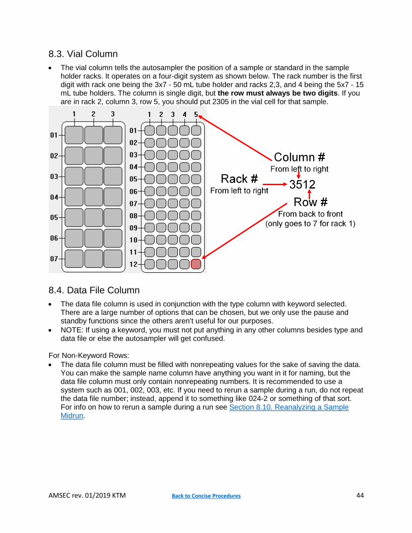
8.3. Vial Column • The vial column tells the autosampler the position of a sample or standard in the sample

holder racks. It operates on a four-digit system as shown below. The rack number is the first digit with rack one being the 3x7 - 50 mL tube holder and racks 2,3, and 4 being the 5x7 - 15 mL tube holders. The column is single digit, but the row must always be two digits. If you are in rack 2, column 3, row 5, you should put 2305 in the vial cell for that sample.

8.4. Data File Column • The data file column is used in conjunction with the type column with keyword selected.

There are a large number of options that can be chosen, but we only use the pause and standby functions since the others aren’t useful for our purposes.

• NOTE: If using a keyword, you must not put anything in any other columns besides type and data file or else the autosampler will get confused.

For Non-Keyword Rows: • The data file column must be filled with nonrepeating values for the sake of saving the data.

You can make the sample name column have anything you want in it for naming, but the data file column must only contain nonrepeating numbers. It is recommended to use a system such as 001, 002, 003, etc. If you need to rerun a sample during a run, do not repeat the data file number; instead, append it to something like 024-2 or something of that sort. For info on how to rerun a sample during a run see Section 8.10. Reanalyzing a Sample Midrun.


8.5. Sample Column • The sample column is for your use to label the standards and sample names. Try to keep

them short with no special characters.

8.6. Dil/Lvl Column • This column is very important. For your standards, the level must start at one and increase

until your most concentrated standard. This will become apparent in Section 9.2. on the DA Method Editor. Your samples must always have a value of 1.000.

8.7. ISTD Conc Column • The ISTD Conc column must always say level one. It is easiest to copy and paste this value

to subsequent cells.

8.8. Helpful Hints • To insert or delete entire lines, simply click on the row number and then right click on the

cell next to it. You can easily insert a copied line this way. • You can have as many samples as the racks will hold. A total of 21 - 50 mL tubes and 180 -

15 mL tubes can be used. • The screenshot above is a good example of how you should set up a sequence. • To learn about running a sequence, see Section 6.2. Analyzing a Sample with a Sequence.


8.9. IMPORTANT: Throwaway Samples There have been recent issues with the autosampler communication to the computer that have resulted in some very unfavorable results. This requires that the autosampler be reset during the very beginning of a run. This also means that if you stop a run in the middle and go to restart it, you will need to add these throwaway samples to run before your second half and for any other time you start a run. This is unavoidable and hopefully can be remedied soon. The steps to take are relatively simple, but must be done precisely. First, you will need to add two throwaway samples to the beginning of your sequence as seen below.

They have been given really high data file names as to avoid interfering with any files related to the samples. Make sure that the vial number is directed to an empty vial slot on the autosampler, this needs to be done to avoid cross contamination. You can have the vial be the same for both throwaway samples if you like. I have put them to the vial slots directly after my standards in this example. Once you begin running your sequence, you will wait until the first throwaway sample gets to the rinse phase and the kill the following tasks in the task manager. You can access the task manager through ctrl+alt+delete and then clicking task manager or, more easily, by pressing ctrl+shift+esc. It is recommended to have the task manager open before your first throwaway gets to the rinse phase. Once it gets to the rinse phase, you must end two tasks in this specific order. First, end “icptune.exe” followed by “icpacq.exe”. This can be done more easily by clicking on the task and pressing the delete key followed by the enter key.


Once this has been done, the acquisition window will disappear from ICPMS Top and you will get a message saying that application 0 has died followed by one that says that application 1 has died. Once you click through these two, the system will resume the sequence and proceed to the second throwaway sample. After this, the sequence will resume its normal function. Notes:

- It can speed up the throwaway samples to click the skip peristaltic pump option. This isn’t necessary as they are just drawing in air. This isn’t required, but can save a few minutes, but shouldn’t ever be done on an actual sample.

- In previous windows there has been a “Rinse Blank” added before the actual calibration blank. This has been shown to improve the initial measurements of the instrument. It may be due to sucking in a lot of air directly before running, but having the blank run twice in a row seems to help. The first time it is ran it is treated as a sample and ignored for actual data analysis.

8.10. Reanalyzing a Sample Midrun There may come a time when a sample has high RSDs all around, or you just want to confirm the data is consistent. In this case, you can add a sample in to run again or add a new sample during a run. This will save time as you don’t have to restart the run and do another set of throwaway samples. Reanalyzing a sample during a run is relatively simple and does not require a lot of detail, simply follow these instructions.

- Click on the button on the right in the analysis window “Edit Sample Log Table”. This is not available when rinsing.

o The sample will not proceed to the next one if you are still editing the sample log table when the current analysis ends, therefore, you should make it a relatively quick change. Usually you have two to three minutes.

- Once in the window you will see the exact same window as your sequence. The greyed out line have already run or it is currently in progress.

- Right click on the line below where you want to insert the new line and choose insert line. You can then copy the method and whatnot from another line.

- Then input the correct method, sample type, vial, data file name (make sure not to use one that has been or will be used, I recommend using the previous data file name with a -2 added), sample name and make sure you have the right Dil/Lvl for the case of a sample or a standard.

- Accept the changes and it will proceed with your run as you have just scheduled.


9. Data Analysis Window This section describes the data analysis window which is new to this version of software. This window communicates with the ICP-MS Top software and displays the data collected from the current run. There are a few slight bugs with this software. It is helpful to see Section 13. Troubleshooting and Error Help.

9.1. Software Overview • The data analysis window can be accessed from the ICP-MS Top window by selecting Main

Panel from the Data Analysis dropdown menu.

• The window that opens should look like the screenshot below. If it doesn’t, click the Default

Layout button on the icon bar. Important features are described below this image.

Important features of the software window include: 1. File Menu: save/create/load/export batches and data 2. Icon Bar:

a. Create a new batch file 3. Data display: displays currently b. Open an existing batch file selected data or ISTD stability c. Save the current batch file plot. d. DA Method Editor 4. Calibration Curve Window: Shows e. Process Batch calibration curves (liquids only). f. Layout bar: choose default layout to return to this layout g. Column bar: choose between display modes-concentration, count, user defined

(1-4 presets) and default columns (default is in conc mode).

1 2

a b c d e f g

3 4


9.2. Batch Files (Liquids) What is a batch file? This is a folder that is read like a file. Yes, you can even open the folder in a file browser and view the contents. This batch file will contain all the data for your standards and samples as well as your calibration curve data. If you back up this file, you will have everything you need to access the data should the file become corrupt. You should save it on the E-drive under the correct folders. 9.2.1. Creating a Batch File Creating the batch file for liquids is extremely important. This is going to determine how well your calibration curves turn out and whether your data is displayed correctly. This is the method for spectrum analysis. If you have already run an analysis with a batch file and want to use the same standards with the same concentrations, select Import DA Method Only under the DA Method Editor and choose the last batch that was ran with those standards. Everything will import for you. • Create a new batch folder and save it in your folder (E:\Data\Research or WWU Classes) • Click on DA Method Editor

• This is how the window should look. Click on Analyte List

The analyst list tells the software what elements you are collecting data for. It will only show data for elements in this list. To populate the list, click Load List From Acquisition Method. Select the method you are using to collect this data and click open. The list should now be populated.


• Once you have your analyte list populated, you must tell the software which elements are internal standards (ISTD). The ISTDs contained within the solution provided by AMSEC are 7Li 45Sc 72Ge 103Rh 115In 159Tb 209Bi and 232Th. Ensure that these elements are selected as ISTD in the analyst list window as shown below. Also ensure that they are selected in your method file. For more information see Section 7.4.1 or 7.4.3 on Acquisition.

• You may only need to select a few of the ISTD elements, this depends on which elements

you are analyzing and this can be clarified in the next step of the DA Method Editor. • Once finished in the Analyte List, select Full Quant under step 4. The window should look

like this.


• In the middle pane there is a lot of information to tell the software about your calibration standards. First, set the units for the concentration under the analyte portion. Commonly used are ppm and mg/L.

• Then add as many levels as you have standards. This includes the blank (with a conc. of 0).

• The default is 5 levels, so add as many as you need. These levels correspond to the levels

in the sequence file and they must match or else the software will label the standards incorrectly. For more information, see Section 8.6 Dil/Lvl Column.

• Next, input the standard concentrations for each element. If you did serial dilutions, there is an easy way to do this. If you did not, then you must manually enter each concentration for each element at each level. Level 1 should be the blank and the highest level should be the most concentrated standard.

• To enter standards via serial dilution. Manually enter the highest standard values for each

element. The software has a concentration multiplier function access by right clicking on the highest level column heading as shown above. Then choose Multiply Conc…

• The level already entered will be multiplied by 1. You can now enter the dilution factor for

each level. The sample shown above is for a ten-fold serial dilution. Click OK.


• The table should now be populated as seen below. It may look different based on how many analytes you have and the concentrations of your standards. Make sure you have set the Units for the standards.

• Now we must select the internal standards for each analyte that will behave similarly in the

ICP-MS. This is almost always the isotope of the closest mass to that of the analyte. Select this for each element you are analyzing. If an internal standard is not used, you may remove it from the analysis and method to reduce acquisition time.

• Next, we will examine the section of this window on ISTDs.

• Select ppm for Units for every ISTD element. Then click the Edit ISTD Conc checkbox and

ensure that every level has a value of 1. Blank levels can cause errors with the software. • Now click Validate on the left of the window. If everything was input correctly, a popup will

appear that says no errors found. Click OK and then click Return to Batch-at-a-Glance. Click Yes to update the Analysis Method.


• You have now created a batch file to collect data with. Be sure to save the file before collecting data as ICP-MS Top won’t collect with an unsaved batch file.


9.2.1 Looking at Data and Calibration Curves An example set of data is shown in this section to give you an idea of what things you can do in this window with your data set. • Assuming you did everything correctly setting up the DA Method, your window may look

similar to this. I have chosen a set with only a few elements of analysis for ease of viewing.

• The data file information is on the left. The elements are listed across the top with an RSD

column. The RSD is the relative standard deviation. It is the st.dev./average x 100. It is a percentage. Any value with an RSD over 5% will be highlighted in pink. You want to minimize this. There was a lot of error in this data set.

• In the bottom left window, the mass spectrum of the highlighted sample is shown. This window isn’t commonly used, but has a useful function if ISTD Stability Plot is selected.

• This shows the counts for the ISTDs over the entire run. This allows for the user to have an

idea of which samples may be suspect for quantification and may need to be ran again. • The bottom right pane of the window shows the calibration curved and ISTD data plots from

the standard data.

ISTD Stability Plot


• The plots with lines are calibration curves for the elements in the title and the plots with just

points show the counts of the ISTD for each standard. A nice grouping is what you want to see. You must investigate each calibration curve to ensure good data. Simply double click on one to expand and investigate. To return to this view, click the grid view button.

• The calibration curve should appear. The table to the right can be brought up by selecting

the button indicated above. You want to try to get an R value as close to 1 as possible. This may be achieved be rejecting a point that isn’t in line with the others. It is possible to reject a few points and maintain the integrity of the data. To do this, click the reject column checkbox or click the point on the sample. To zoom in, use right click to drag a box around the area of interest. To zoom out, right click and select autoscale.

• You need to go through every calibration curve to ensure good data. This can be done after samples have been run, but if the standards didn’t turn out well, then the instrument or the standards may need some fine tuning or to be remade. It is recommended to review them right after they finish as to not waste time and sample.

• If the Process Batch button is ever red, you must click it and then save the batch file. This can be done after a series of calibration curve alterations. This recalculates all quant data.

Grid View

Autoscale Plot Navigate Pages

Navigate Samples

Analyte of this cal curve

Corresponding ISTD


9.3. Exporting and Viewing Data (Liquids) In order to export the data, you need to be able to view the data in different ways. Some people only want the quantified data, some want the average counts per second (CPS), but some users will want all the data for every replicate. 9.3.1. Average CPS View • To view the average CPS for each element, select Default Columns followed by the Count

button.

• The result should look like this:

9.3.2. Concentration View • To view the calculated concentration, select Default Columns followed by the Conc button.

• The result should look like this:

• Note that the ISTD values are blank. Since the Conc values are based off these, no value

can show up here. They are always 1 ppm.


9.3.3. Total Replicate View • To view all the replicates for each element, select User Setting 4 (directly left of Default

Columns). This will show all the replicates along with the calculated average for each element. This may look very different for each user so no screenshot is displayed. There are a couple other user setting that have been programmed in. Try them out to see if this will be good for you. Once you click user setting 4, it will look as seen below.

• During the export, the presence of the checkboxes will cause an error in exporting that

will say something about the limit of Excel’s columns. This can be remedied by right clicking on the column header and unchecking the option for “Reject Column For Replicate Data”. This will remove all the checkboxes and allow you to export the data normally.


9.3.4. Exporting Data • To export data, you must have it displayed as you would like it to be exported into excel.

This means looking at the last three sections and deciding which ones you want to analyze. You may do as many as you like.

• To export, right click on the data table heading or click the File menu. Go to export and

select which option you would like. Most users prefer Export Table. You can also export only selected samples and elements with Export Selected Area.

• Try out as many combinations as you want. They are all separate excel files so there is no downside to experimenting.


9.4. Batch Files (Laser Ablation) What is a batch file? This is a folder that is read like a file. Yes, you can even open the folder in a file browser and view the contents. This batch file will contain all the data for your standards and samples as well as your calibration curve data. If you back up this file, you will have everything you need to access the data should the file become corrupt. You should save it on the E-drive under the correct folders. 9.4.1. Creating a Batch File (Time Resolved Analysis) For time resolved analysis with laser ablation, the Data Analysis window has less of an important function and acts mainly as an organizational tool. It also allows you to come back at any time to export data if you have lost or forgotten your files. • Create a new batch folder and save it in your folder (E:\Data\Research or WWU Classes) • Click on DA Method Editor

• Change the analysis mode from Spectrum to Timechart. Then click on Analyte List on the

left-hand side.


• Next, click on Return to Batch-at-a-Glance. A dialogue will appear asking to update the DA

Method. Click Yes.

• You have now created a batch file to collect data with. Be sure to save the file before

collecting data as ICP-MS Top won’t collect with an unsaved batch file.



9.4.2. Creating a Batch File (Spectrum) For spectrum analysis of laser ablation samples, the Data Analysis window has less of an important function and acts mainly as an organizational tool. It also allows you to come back at any time to export data if you have lost or forgotten your files. • Create a new batch folder and save it in your folder (E:\Data\Research or WWU Classes) • Click on DA Method Editor

• The window will look as shown above. Click on Analyte List on the left-hand side.

• Next, click on Return to Batch-at-a-Glance. A dialogue will appear asking to update the DA

Method. Click Yes.



• You have now created a batch file to collect data with. Be sure to save the file before

collecting data as ICP-MS Top won’t collect with an unsaved batch file.


9.5. Exporting and Viewing Data (Laser Ablation) This may not be necessary if you chose the option to tabulate chart to CSV in your method information. If you did this, simply go to your batch folder in a file browser and search “.csv” and all of your files will show up. 9.5.1. Time Resolved Analysis • To properly view data in time resolve analysis mode. Select Default Columns followed by the

Count option to the left.

• The window should look as seen below:

• The data shows only the first data point in the table. The actual time plot is shown on the bottom left. This window can be expanded and you can even close the bottom right window which has no function for this analysis mode. If this isn’t present, press default layout.

• To export data, highlight an entire sample by clicking on the row number. Then right click on the time chart in the bottom left pane. Choose Tabulate Chart CPS Data to CSV.


• Once selected, an excel sheet will open with the tabulated data. A filepath is shown at the top which shows where this data file is saved.

• You must select each sample individually and tabulate all samples that you run. This can be

done as you go or all at the end if you did not choose the option to tabulate chart to CSV in the method info.

• You can use save as to save each individual file to a location of your choosing. The other option is to extract all these files from the file browser. Simply open a file browser and navigate to your batch folder. Then, open your batch folder and use the search bar in the top right to search “.csv”. All the CSVs in that folder will show up and you can copy paste them to your own save location such as a flash drive.

Search Bar


9.5.2. Spectrum Analysis It may help to read the section on Exporting Data for Liquids. This might show other useful options you may need. • To properly view data in spectrum mode. Select Default Columns followed by the Count

option to the left.

• The window should look as seen below:

• The data is shown for each element and the actual spectrum is in the bottom left pane. The

bottom right pane has no use for this type of analysis.

• To export, right click on the data table heading or click the File menu. Go to export and

select which option you would like. Most users prefer Export Table. You can also export only selected samples and elements with Export Selected Area.

• Try out as many combinations as you want. They are all separate excel files so there is no downside to experimenting.


10. Tuning the Instrument We do not typically allow students to tune the instrument. This is for various reasons and

mainly maintains the integrity of the data you are collecting and allows for the tracking of the tune values over time to monitor changes in instrument parameters. The only exception to this is that when switching from laser to liquids mode you must do a P/A Factor tune.

10.1. Selecting a Tune File • Before running a sample you must select the appropriate tune file for the mode you are

running in. To do this, open the Tune Panel. See Section 6. General Software Overview for more information.

• The Tune Panel will look like this:

• The parameters that are displayed when you open the tune panel are the ones that were

used last and it will always say atune.u. When you select a tune file and close the window, atune.u is populated with those tune values and is used by the instrument. Do not be alarmed if you had loaded a tune file and when the window reopened it said atune.u.

• To load the tune file you need, check if it is in the dropdown box or click File Load Tune File or click the open folder. Select the proper tune file. If you are doing laser ablation, choose LATUNE.U for standard mode or select whatever tune file you need to. For liquids, select either nogas.u, he.u, or h2.u depending on what mode you are running in. For standard mode without the ORS, choose nogas.u. For helium of hydrogen mode with the ORS, select he.u or h2.u, respectively.

• For liquids, you will want to rinse the probe before starting any runs or any tuning. To do this, simply choose rinse from the ALS drop down menu. After about 30 seconds and ensuring that the rinse water has made it through the pump, choose ALSHome.


10.2. P/A Factor Tuning (Liquids) • When switching from laser ablation to liquids, you must perform a P/A Factor tune. To do

this, set up the hardware and uncap the P/A tune solution. For more help on hardware setup, see Section 3. Hardware Setup and Section 5.1. Setting up the Hardware. For the P/A tune, the ISTD tube must be in the 2% nitric bottle. See Section 5.1.3. Internal Standard Tubing Setup for more information.

• Make sure to have rinsed the probe prior to this. To do this, simply choose rinse from the ALS drop down menu. After about 30 seconds and ensuring that the rinse water has made it through the pump, choose ALSHome.

• Load the method file P_A.M by selecting Method Load. Enter the Tune Panel and load nogas.u. For more help see Section 10.1. Selecting a Tune File.

• Select Tune P/A Factor. A dialogue box will appear. Click the following:

o Load masses from acquisition method o Make sure the tune vial is selected with the P/A solution in it. It is usually in 5. Make

sure all the rinse vials are open. o Click ok

• The tune will automatically commence. Once it is done, a dialogue will appear that asks if you want to adopt the new factors. To decide whether they should be adopted or not, look at the report pad that has opened. You should see no more than 6 elements without a number value. If that is the case, select yes to adopt the new factors. If that is not the case, select no and contact the lab manager for more help.

• Be sure to recap the tune solution and load the appropriate tune file you need. Also, remember to load the method you need before continuing to run samples.


11. Preferred Isotopes and Interferences This section will describe a few simple explanations and examples of what isotopes are preferred and some common interferences. The periodic table on the next page is a good starting point for anyone to use, but does not apply to everyone’s samples or matrices. You will need to use your best judgment when choosing what isotopes to choose and how to avoid interferences. If you routinely have problems with interferences, or you aren’t sure, talk to your research advisor or the lab manager for more information. Interference equations may be useful in this case. Things to consider when choosing isotopes:

• What things will add up to the same mass as my sample? Is there a lot of this? o This can help you narrow down if there will even be an issue. For example, if I

am worried about MgO interfering with my phosphorous 30, but there is negligible amounts of magnesium in my sample, then I can probably ignore this and use the helium ORS mode to completely remove this.

• What isotopes have overlap with other elements? Will there be a lot of this overlapping element?

o If I am trying to study 118In, but there also exists a 118Sn, then I don’t have to worry if there is no tin in my sample, but if there is, I may have to consider other options.

• Do I need to use helium or hydrogen in the ORS? Will this completely remove the interference or will I still have to worry about it?

o If the interference masses are heavily prevalent, then you cannot remove them completely. Most of the time it is easier to choose a different isotope. If this is not possible, talk to your research advisor or the lab manager for help.

• What other isotopes can I run for a selected element? Do I have many options and what are the natural abundances of these? If the abundance is extremely small, it will not be a good choice.

o An example of this is iron. 56Fe has a major interference with ArO. As those elements are very prevalent, we cannot remove this interference. We can look at the other isotopes of iron. 58Fe is only 0.282% abundant and therefore is a poor choice when compared to 57Fe which is 2.119% abundant. This means we should choose to analyze 57Fe over 56Fe for interference reasons and 56Fe over 58Fe for abundance reasons.

This type of questioning and reasoning should be applied to every choice of isotope you make. This can often be a lengthy process and this is why method development is crucial to getting good results and understanding what is happening inside the instrument. A good resource for looking at isotopes of each element with a lot of information can be found at PTable.com and then select the isotope tab. Link provided.

http://www.ptable.com/#Isotope


12. Shutting Down the Instrument 12.1. Shutting Down with Liquids To shut down the instrument follow these steps. Most of them are reverse of the setup procedure. 1. Put the ISTD tubing into the 2% Nitric bottle 2. Release the black peripump clamps and relieve the tension on the three tubes by unhooking

them. 3. Send the autosampler probe home from the instrument control or tune panel. ALS Home 4. Turn off the autosampler and release the peripump tube clamp on the back. 5. Close all the rinse bottles. 6. Shut off the plasma if not already done from the instrument control window.

Select Plasma Plasma off 7. Turn of the argon. 8. Turn off the water chiller. Wait at least 10 minutes after turning off the plasma to do this.

(ES 128B) 9. Remove your samples and clean up any mess. 10. Notify the lab manager if anything needs to be repaired or replaced.

12.2. Shutting Down with Laser Ablation To shut down the instrument follow the following steps. Most of them are reverse of the setup procedure. 1. Shut off the plasma from the instrument control window.

Select Plasma Plasma off 2. Remove your sample from the laser ablation accessory. 3. Turn the He flow off in the laser ablation software. 4. Shut off the argon tank. 5. Turn off the water chiller. Wait at least 10 minutes after turning off the plasma to do this.

(ES 128B)


13. Troubleshooting and Error Help If you have an error or something goes wrong. Try to find a solution in the following pages or do some basic troubleshooting to determine the cause. If you can’t find anything helpful and resolve the issue by yourself, contact the lab manager and they will assist with the problem.

13.1. Plasma Ignition If the plasma won’t light or shuts off, check the following: Is the Argon tank on and is there 100 psi output shown on the left gauge of the regulator?

- If not, open the tank and use the knob on the regulator to increase the pressure to 100 psi if necessary.

- Check that the valve on the far left of the regulator is open. - Check that the liquid argon tank has sufficient internal pressure. See the section on

Liquid Argon Tank Operation for more information. Is the Argon tank empty?

- If the tank valve is open and the required pressure cannot be obtained, the tank may be empty.

- Let the lab manager know so they can order a new one. - Change the regulator from the liquid tank to the compressed argon tank located nearby.

It has a sticker on it that says argon and should have a cap on the tank as well. These tanks are normally red.

- If you have trouble with this the lab manager can help. If they are not around, try to find another person who knows how to change a regulator.

Is the water chiller on?

- Typically if the water chiller isn’t on, you will get an error specifying insufficient cooling water flow.

- Simply go into the adjoining room (ES 128B) and turn on the chiller. Is the helium flow too high? (Laser Ablation only)

- If the helium flow is too high to start, the plasma may not light. - Turn the flow to 50 mL/min and try to light again. After the plasma is fully lit, increase the

flow slowly (by using the up arrow on the mass flow control panel) to the desired set point.

Did you hook up the drain tubing correctly?

- If the drain tubing wasn’t hooked up correctly, the plasma chamber may be flooded. - If this is the case, contact the lab manager as this will require cleaning and the

instrument may be offline for a couple days. If the plasma will not light after following these troubleshooting steps, try to write down the error produced when it shuts off or doesn’t light and inform the lab manager.


13.2. Pumping Issues (Liquids Only) If there are issues with your solution pumping. Try the following steps. Are there any kinks in any of the lines?

- Check for any kinks or turns in the line that are too sharp and try to straighten them out. Is the peristaltic pump hooked up correctly?

- The direction of the tubes hookup and the proper hookup are important. See Section 5.1.1 Peristaltic Pump Setup for more information.

Did any of the tubing come undone?

- Occasionally the tubing comes undone and the solution will be pumped out onto the tray. Check if this is the case and then look at the next question before proceeding.

- Using gloves, hook up the tubing as it should be and push the disconnected tubing back together.

Is the nebulizer clogged?

- Look at the nebulizer where the tube goes in and look for anything that looks like a clog. Sometimes they are small and not very noticeable.

- If you find a clog, report it to the lab manager. The instrument is not usable until this is resolved.

13.3. Issues with Batch Files Some users experience issues with batch files saving and communicating with the ICP-MS Top software. Some common issues and resolutions are listed below. For more information see Section 9. Data Analysis Window for more help with your respective analysis type. Is the data not showing up after an acquisition finishes?

- Check to see that your DA Method is set up correctly. See Section 9. Data Analysis Window for more help.

- Is the proper display type selected? Choose from the different options on the right side of the toolbar to get either counts or concentrations to show up. It helps to select “Default Columns” and then count or conc mode.

Is the batch file not communicating with the ICP-MS Top software?

- Most of the time, this is due to a batch file name being too long and containing special characters. Limit the total character count to 8 and only use letters and numbers. Most of the time it is suggested to use the current date. (i.e. 05142015.b)

- If you made a complicated batch file name and tried to run a sample, you may have to restart the computer before you will be able to use the new, shorter named batch file to collect data. The ICP-MS will stay running while the computer restarts.


13.4. Data not Displaying at all in the Data Analysis Window The DA Method editor can be a finicky portion of the DA window. If this is not set up correctly, your data may not show up at all, but fear not! The data is in the file, it just isn’t displaying due to a configuration error. See Section 9. Data Analysis Window for more help with this. Is your data analysis type set correctly for your analysis method?

- If you are running a time resolved analysis you need to change to timechart in the DA Method Editor under Data Analysis Method.

- If you are running a spectrum mode, you must ensure this is selected in the DA Method Editor under Data Analysis Method.

Is the Analyte List correctly populated?

- Check that you have imported your analyte list from your method file. In the DA Method Editor, select Analyte List and at the top choose Load List from Acquisition Method. Select your method.

- (Liquids) Once the analyte list is loaded, be sure to set the internal standards. For a list and instructions on this, see Section 9.2.1 Creating a Batch File.

13.5. Issues with Noisy Data and High Backgrounds Occasionally, the instrument will output really noisy data and the background signals will be very high and unstable or drop out suddenly. Try the following to remedy this. If this doesn’t work, contact the lab manager. The other possibility for noisy signals is sample contamination or dirty tubing. Does the background signal drop out for no reason?

- Try restarting the plasma to see if there is a torch grounding issue. If this does not work, try once more.

- See if the gas flows are consistent. Go to the instrument control panel and monitor the gas flows using the meters.

Is there a high background?

- (Liquids) Try rinsing the tubing with a 5% nitric solution to try to clear out the lines. If this doesn’t work, the lines may need to be changed or your blank is too dirty.

- (Laser Ablation) Try letting the instrument warm up for longer with the helium flowing at the rate at which you wish to capture. Watch for the signals plateau with no slope such that the background is constant.

- (Laser Ablation) Allow more time between sample runs as there may be residual sample in the line that needs to be purged between acquisitions.

icpms standard operating procedures-liquids contents · the argon plasma is capable of breaking...

Documents