iconip’2008 tutorial on computational resources in neural ...sima/tutresnn.pdf · iconip’2008...
TRANSCRIPT
ICONIP’2008 Tutorial on
Computational Resources
in Neural Network Models
Jirı Sıma
Institute of Computer ScienceAcademy of Sciences of the Czech Republic
(Artificial) Neural Networks (NNs):
1. mathematical models of biological neural systems
• constantly refined to reflect current neurophysiologi-cal knowledge
• modeling the cognitive functions of human brain
already first computer designers sought their inspirationin human brain (neurocomputer, Minsky,1951) −→
2. computational tools
• alternative to conventional computers
• learning from training data
• one of the standard tools in machine learning and datamining
• used for solving artificial intelligence tasks: patternrecognition, control, prediction, decision, signal anal-ysis, fault detection, diagnostics, etc.
• professional software implementations (e.g. Matlab,
Statistica modules)
• successful commercial applications
Neural Networks asAbstract (Formal) Computational Models
• mathematically defined computational machines
• idealized models of practical NNs from engineeringapplications, e.g. analog numerical parameters are truereal numbers, the potential number of computationalunits is unbounded, etc.
• investigation of computational potential and limits ofneurocomputing
special-purpose NNs: implementations of neural circuitsfor specific practical problems (e.g. robot control, stockpredictions, etc.)
× general-purpose computation with NNs:
• the study of classes of functions (problems) that canbe computed (solved) with various NN models(e.g. XOR cannot be computed by a single perceptron)
• what is ultimately or efficiently computable byparticular NN models?
analogy to computability and complexity theory of con-ventional computers (PCs) with classical abstract com-putational models such as Turing machines (recursivefunctions), finite automata (regular languages), etc.
−→ Computability and Complexity Theory ofNeural Networks
• methodology: the computational power end efficiencyof NNs is investigated by comparing their variousformal models with each other and with more tradi-tional computational models such as finite automata,grammars, Turing machines, Boolean circuits, etc.
• NNs introduce new sources of efficient computation:energy, analog state, continuous time, temporal cod-ing, etc. (in addition to usual complexity measuressuch as computation time and memory space)
−→ NNs may serve as reference models for analyzingthese non-standard computational resources
• NN models cover basic characteristics of biologicalneural systems: plenty of densely interconnectedsimple computational units
−→ computational principles of mental processes
Three Main Directions of Research:
1. learning and generalization complexity:effective creation and adaptation of NN representation
e.g. how much time is needed for training? how manytraining data is required for successful generalization?
2. descriptive complexity:memory demands of NN representation
e.g. how many bits are needed for weights?
3. computational power:effective response of NNs to their inputs
e.g. which functions are computable by particular NNmodels?
Tutorial Assumptions:
• no learning issues, this would deserve a separate sur-vey on computational learning theory, e.g. ProbablyApproximately Correct (PAC) framework, etc.
• only digital computation: binary (discrete) I/O values,may be encoded as analog neuron states and interme-diate computation may operate with real numbers
× NNs with real I/O values are studied in theapproximation theory (functional analysis)
Technical Tools (5-slide discursion)
1. Formal Languages and Automata Theory
formal language = set of words (strings) over an alphabet,for simplicity assume binary alphabet L ⊆ 0, 1∗
L corresponds to a decision problem: L contains allpositive input instances of this problem,
e.g. for the problem of deciding whether a given naturalnumber is a prime, the corresponding language PRIMEcontains exactly all the binary expressions of primes
(deterministic) finite automaton (FA) A recognizing alanguage L = L(A):
• reads an input string x ∈ 0, 1∗ bit after bit
• a finite set of internal states (including a start stateand accepting states)
• transition function (finite control):
qcurrent , xi 7−→ qnew
given a current internal state and the next input bit,produces a new internal state
• x belongs to L if A terminates in an accepting state
FA recognize exactly regular languages described byregular expressions (e.g. (0 + 1)∗000; × 0n1n ; n ≥ 1is not regular)

Turing machine (TM) = finite automaton (finite control)
+ external unbounded memory tape
• the tape initially contains an input string
• the tape is accessible via a read/write head which canmove by one cell left or right
• transition function (finite control):
qcurrent , xread 7−→ qnew , xwrite , head move
given a current internal state and a bit on the tapeunder head, produces a new internal state, a rewritingbit, and the head move (left or right)
e.g. TM (in contrast to FA) can read the input repeatedlyand store intermediate results on the tape
TMs compute all functions that are ultimately computablee.g. on PCs (recursive functions)
−→ widely accepted mathematical definition of“algorithm” (finite description)
2. Complexity Theory
• what is computable using bounded computationalresources, e.g. within bounded time and memory
−→ the time and space complexity
• the complexity is measured in terms of input length(potentially unbounded)
• TM working in time t(n) for inputs of length nperforms at most t(n) actions (computational steps)
worst case complexity: also the longest computationover all inputs of length n must end within time t(n)(× average case analysis)
• TM working in space s(n) for inputs of length n usesat most s(n) cells of its tape
“big-O” notation:e.g. t(n) = O(n2) (asymptotic quadratic upper bound):there is a constant r such that
t(n) ≤ r · n2
for sufficiently large n, i.e. the computation time growsat most quadratically with the increasing length of inputs
similarly lower bound t(n) = Ω(n2) (t(n) ≥ r · n2): thecomputation time grows at least quadratically
t(n) = Θ(n2) iff t(n) = O(n2) and t(n) = Ω(n2)

Famous Complexity Classes:
P is the class of decision problems (languages) that aresolved (accepted) by TMs within polynomial time,i.e. t(n) = O(nc) for some constant c−→ considered computationally feasible
NP is the class of problems solvable by nondeterministicTMs within polynomial time
nondeterministic TM (program) can choose from e.g.two possible actions at each computational step
−→ an exponential number of possible computationalpaths (tree) on a given input (× a single deterministiccomputational path)
definition: an input is accepted iff there is at least oneaccepting computation
example: the class of satisfiable Boolean formulas SAT isin NP: a nondeterministic algorithm “guesses” an assign-ment for each occurring variable and checks in polyno-mial time whether this assignment satisfies the formula
−→ NP contains all problems whose solutions (once non-deterministically guessed) can be checked in polynomialtime
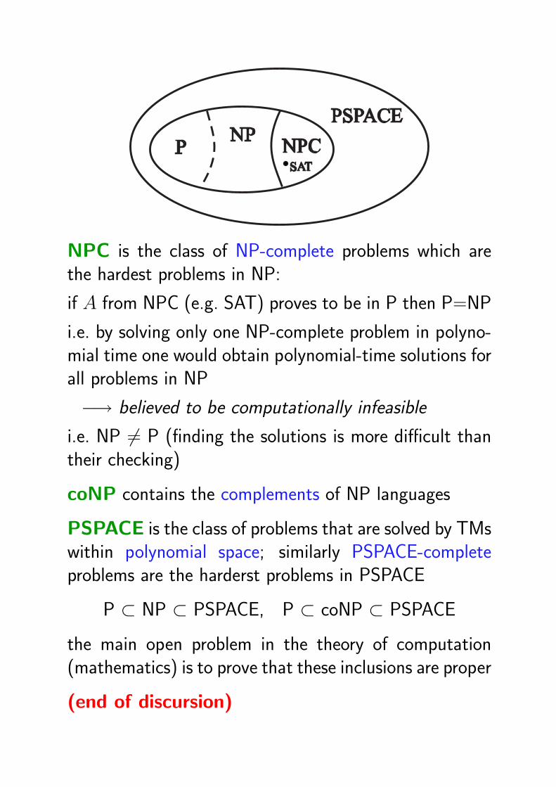
NPC is the class of NP-complete problems which arethe hardest problems in NP:
if A from NPC (e.g. SAT) proves to be in P then P=NP
i.e. by solving only one NP-complete problem in polyno-mial time one would obtain polynomial-time solutions forall problems in NP
−→ believed to be computationally infeasible
i.e. NP 6= P (finding the solutions is more difficult thantheir checking)
coNP contains the complements of NP languages
PSPACE is the class of problems that are solved by TMswithin polynomial space; similarly PSPACE-completeproblems are the harderst problems in PSPACE
P ⊂ NP ⊂ PSPACE, P ⊂ coNP ⊂ PSPACE
the main open problem in the theory of computation(mathematics) is to prove that these inclusions are proper
(end of discursion)

Definition of a Formal Neural Network Model(sufficiently general to cover almost all practical NNs, will later be
narrowed to specific NNs)
• Architecture: s computational units (neurons) V =1, . . . , s connected into a directed graph
−→ s = |V | is the size of the network
• Interface: n input and m output units, the remainingones are called hidden neurons
• each edge from i to j is labeled with a real weight wji
(wji = 0 iff there is no edge (i, j))
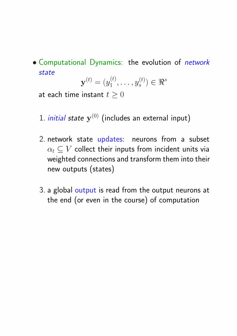
• Computational Dynamics: the evolution of networkstate
y(t) = (y(t)1 , . . . , y(t)
s ) ∈ <s
at each time instant t ≥ 0
1. initial state y(0) (includes an external input)
2. network state updates: neurons from a subsetαt ⊆ V collect their inputs from incident units viaweighted connections and transform them into theirnew outputs (states)
3. a global output is read from the output neurons atthe end (or even in the course) of computation
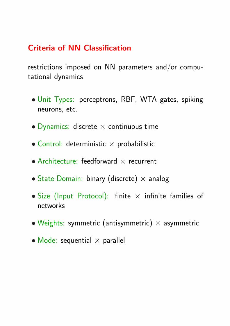
Criteria of NN Classification
restrictions imposed on NN parameters and/or compu-tational dynamics
• Unit Types: perceptrons, RBF, WTA gates, spikingneurons, etc.
• Dynamics: discrete × continuous time
• Control: deterministic × probabilistic
• Architecture: feedforward × recurrent
• State Domain: binary (discrete) × analog
• Size (Input Protocol): finite × infinite families ofnetworks
•Weights: symmetric (antisymmetric) × asymmetric
•Mode: sequential × parallel
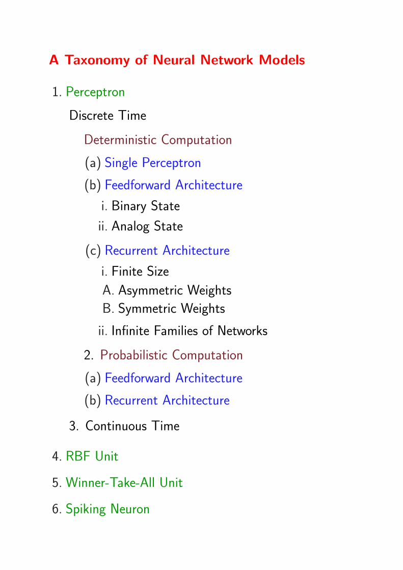
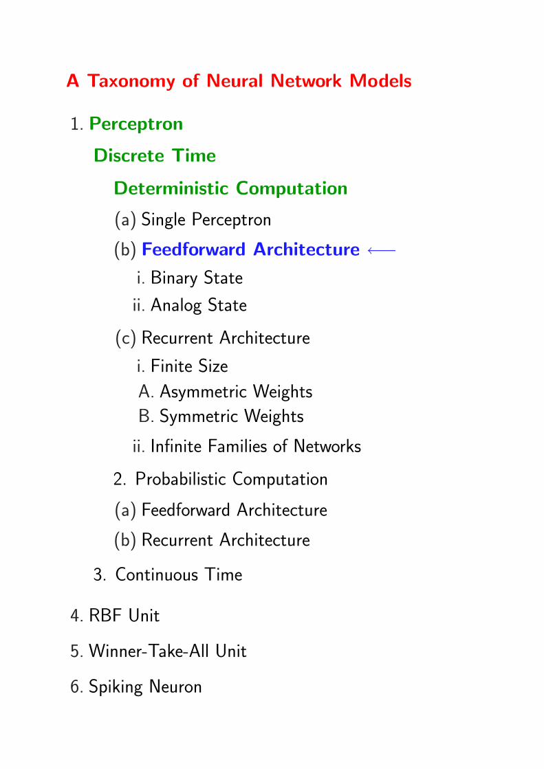
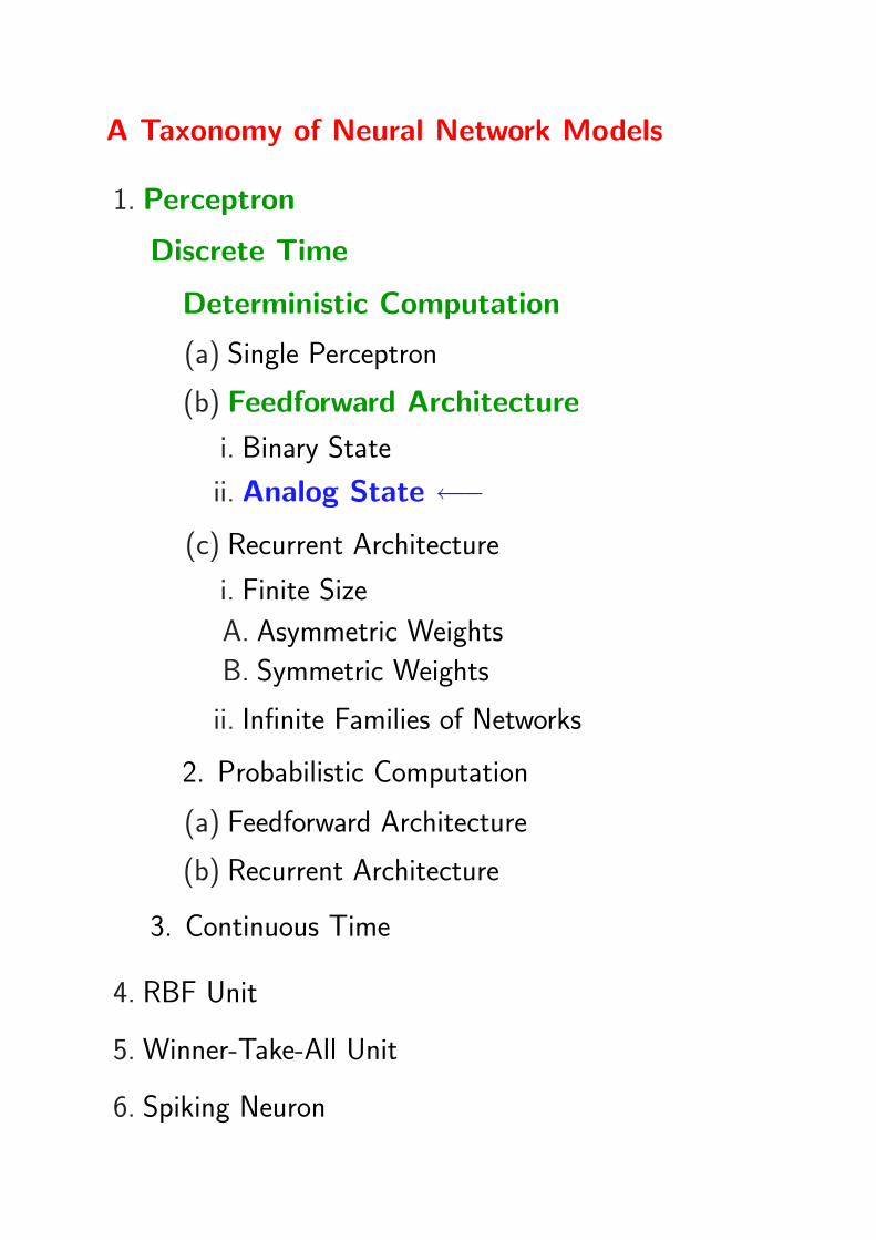
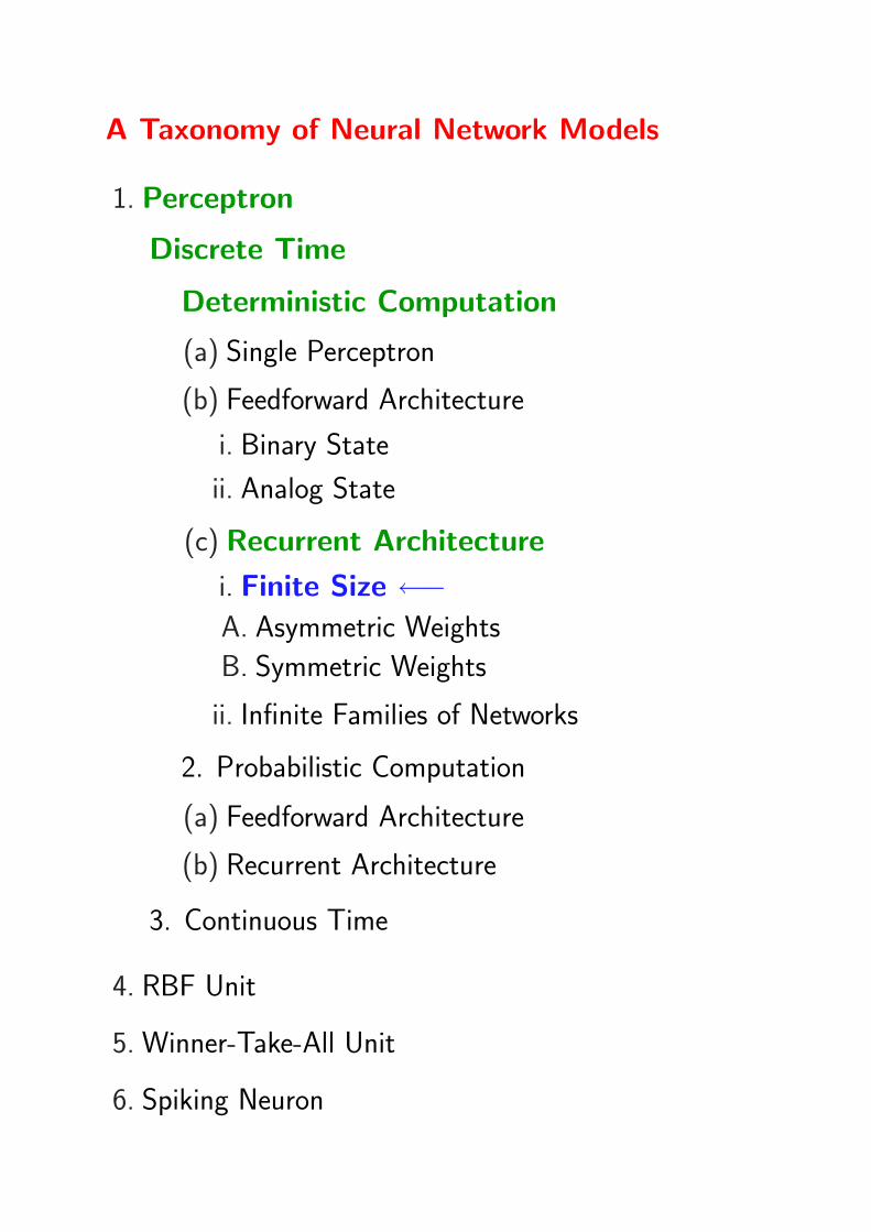
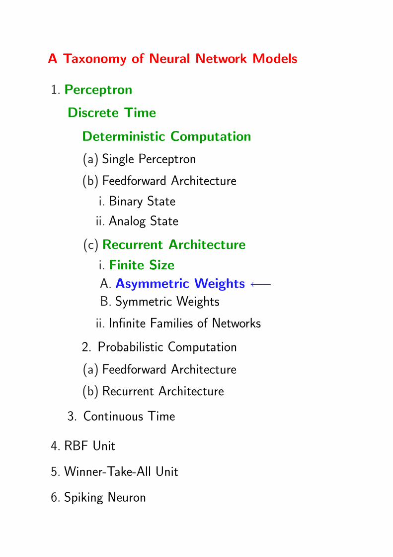
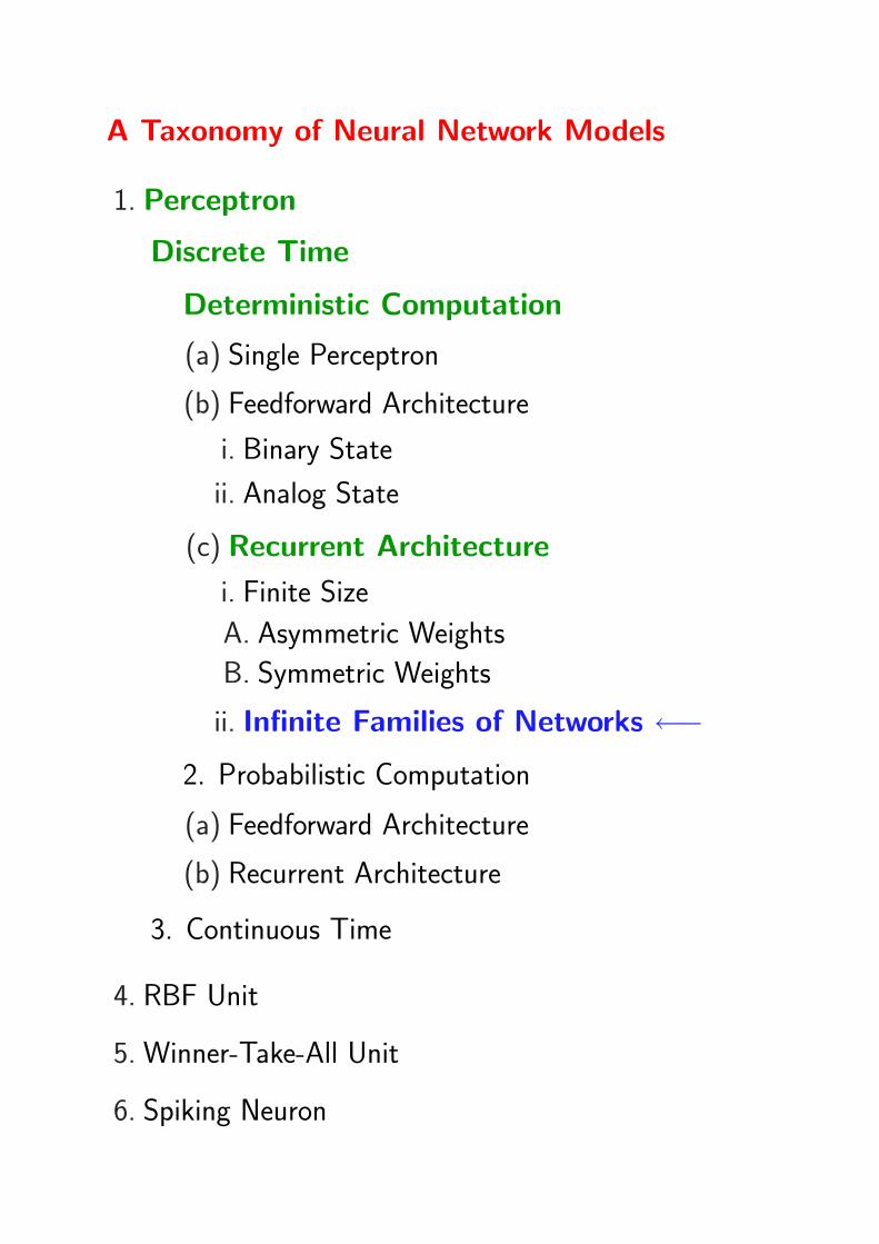
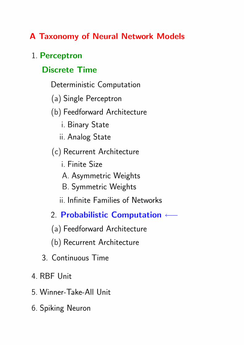
A Taxonomy of Neural Network Models
1. Perceptron
Discrete Time
Deterministic Computation
(a) Single Perceptron
(b) Feedforward Architecture
i. Binary State
ii. Analog State
(c) Recurrent Architecture
i. Finite Size
A. Asymmetric Weights
B. Symmetric Weights
ii. Infinite Families of Networks
2. Probabilistic Computation
(a) Feedforward Architecture
(b) Recurrent Architecture
3. Continuous Time
4. RBF Unit
5. Winner-Take-All Unit
6. Spiking Neuron
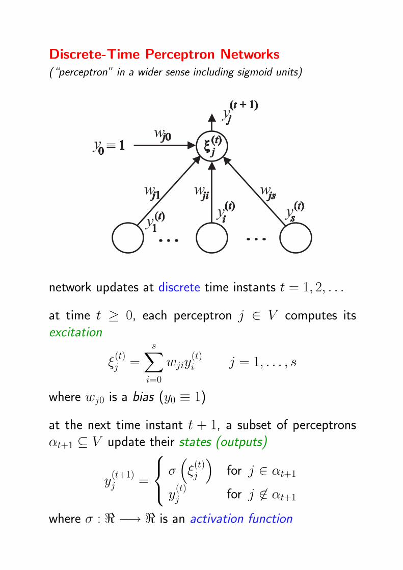
Discrete-Time Perceptron Networks(“perceptron” in a wider sense including sigmoid units)
network updates at discrete time instants t = 1, 2, . . .
at time t ≥ 0, each perceptron j ∈ V computes itsexcitation
ξ(t)j =
s∑i=0
wjiy(t)i j = 1, . . . , s
where wj0 is a bias (y0 ≡ 1)
at the next time instant t + 1, a subset of perceptronsαt+1 ⊆ V update their states (outputs)
y(t+1)j =
σ(ξ
(t)j
)for j ∈ αt+1
y(t)j for j 6∈ αt+1
where σ : < −→ < is an activation function
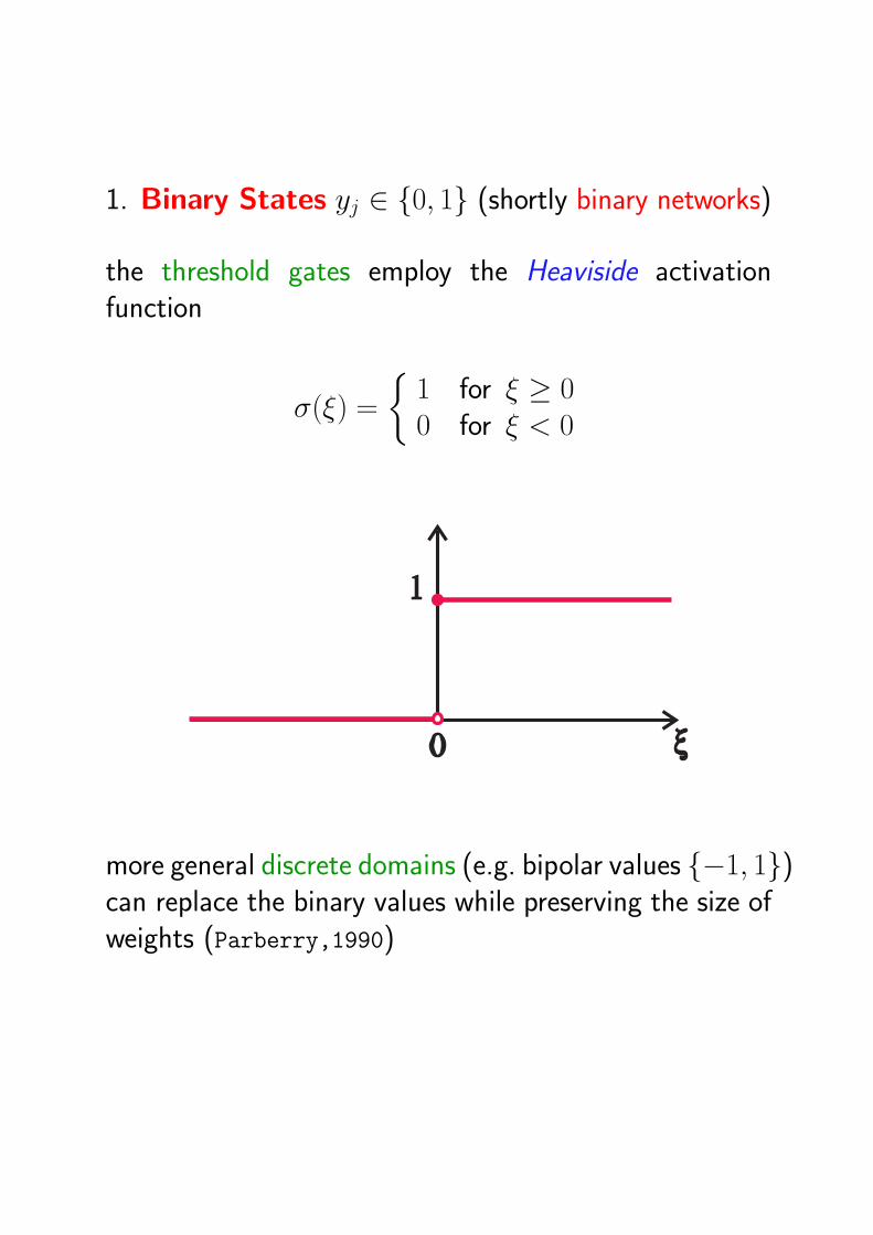
1. Binary States yj ∈ 0, 1 (shortly binary networks)
the threshold gates employ the Heaviside activationfunction
σ(ξ) =
1 for ξ ≥ 00 for ξ < 0
more general discrete domains (e.g. bipolar values −1, 1)can replace the binary values while preserving the size ofweights (Parberry,1990)
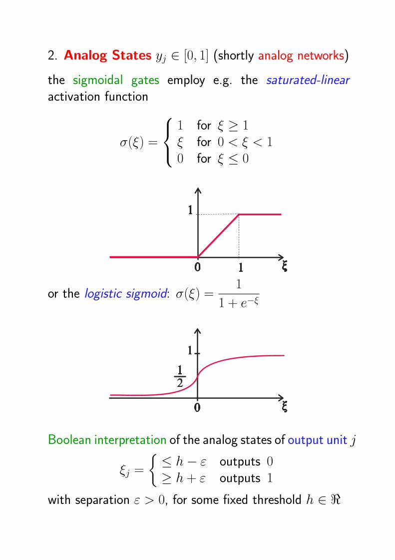
2. Analog States yj ∈ [0, 1] (shortly analog networks)
the sigmoidal gates employ e.g. the saturated-linearactivation function
σ(ξ) =
1 for ξ ≥ 1ξ for 0 < ξ < 10 for ξ ≤ 0
or the logistic sigmoid: σ(ξ) =1
1 + e−ξ
Boolean interpretation of the analog states of output unit j
ξj =
≤ h− ε outputs 0≥ h + ε outputs 1
with separation ε > 0, for some fixed threshold h ∈ <

A Taxonomy of Neural Network Models
1. Perceptron
Discrete Time
Deterministic Computation
(a) Single Perceptron ←−(b) Feedforward Architecture
i. Binary State
ii. Analog State
(c) Recurrent Architecture
i. Finite Size
A. Asymmetric Weights
B. Symmetric Weights
ii. Infinite Families of Networks
2. Probabilistic Computation
(a) Feedforward Architecture
(b) Recurrent Architecture
3. Continuous Time
4. RBF Unit
5. Winner-Take-All Unit
6. Spiking Neuron
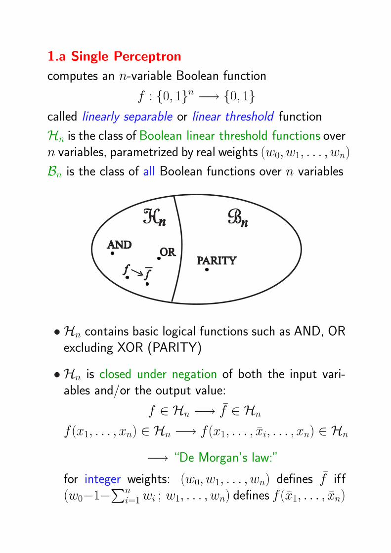
1.a Single Perceptron
computes an n-variable Boolean function
f : 0, 1n −→ 0, 1called linearly separable or linear threshold function
Hn is the class of Boolean linear threshold functions overn variables, parametrized by real weights (w0, w1, . . . , wn)
Bn is the class of all Boolean functions over n variables
• Hn contains basic logical functions such as AND, ORexcluding XOR (PARITY)
• Hn is closed under negation of both the input vari-ables and/or the output value:
f ∈ Hn −→ f ∈ Hn
f (x1, . . . , xn) ∈ Hn −→ f (x1, . . . , xi, . . . , xn) ∈ Hn
−→ “De Morgan’s law:”
for integer weights: (w0, w1, . . . , wn) defines f iff(w0−1−∑n
i=1 wi ; w1, . . . , wn) defines f (x1, . . . , xn)

• the number of n-variable linearly separable functions
|Hn| = 2Θ(n2) ¿ 22n= |Bn| (Cover,1965; Zuev,1989)
−→ limn→∞|Hn||Bn| = 0
• to decide whether a Boolean function given in (disjun-ctive or conjunctive normal form) is linearly separable,is coNP-complete problem (Hegedus,Megiddo,1996)
• any n-variable linearly separable function can beimplemented using only integer weights (Minsky,Papert,1969), each within the length of
Θ(n log n) bits
(Muroga et al.,1965; Hastad,1994)
A Taxonomy of Neural Network Models
1. Perceptron
Discrete Time
Deterministic Computation
(a) Single Perceptron
(b) Feedforward Architecture ←−i. Binary State
ii. Analog State
(c) Recurrent Architecture
i. Finite Size
A. Asymmetric Weights
B. Symmetric Weights
ii. Infinite Families of Networks
2. Probabilistic Computation
(a) Feedforward Architecture
(b) Recurrent Architecture
3. Continuous Time
4. RBF Unit
5. Winner-Take-All Unit
6. Spiking Neuron
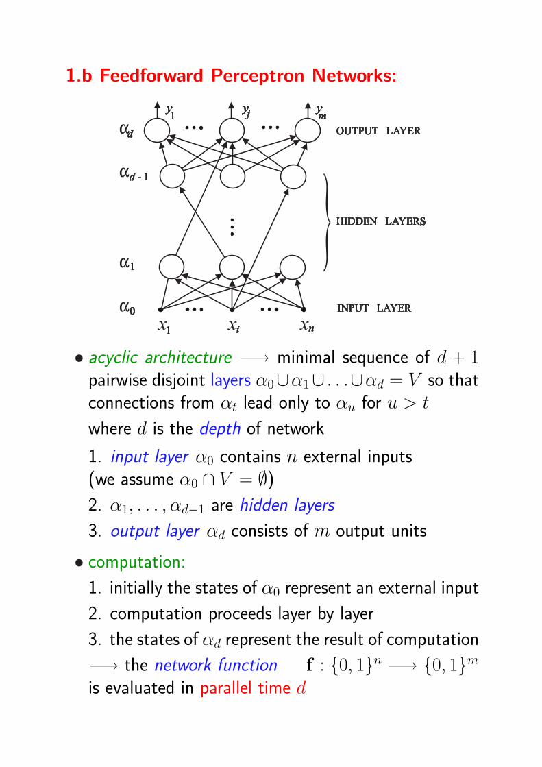
1.b Feedforward Perceptron Networks:
• acyclic architecture −→ minimal sequence of d + 1pairwise disjoint layers α0∪α1∪ . . .∪αd = V so thatconnections from αt lead only to αu for u > t
where d is the depth of network
1. input layer α0 contains n external inputs(we assume α0 ∩ V = ∅)2. α1, . . . , αd−1 are hidden layers
3. output layer αd consists of m output units
• computation:
1. initially the states of α0 represent an external input
2. computation proceeds layer by layer
3. the states of αd represent the result of computation
−→ the network function f : 0, 1n −→ 0, 1mis evaluated in parallel time d
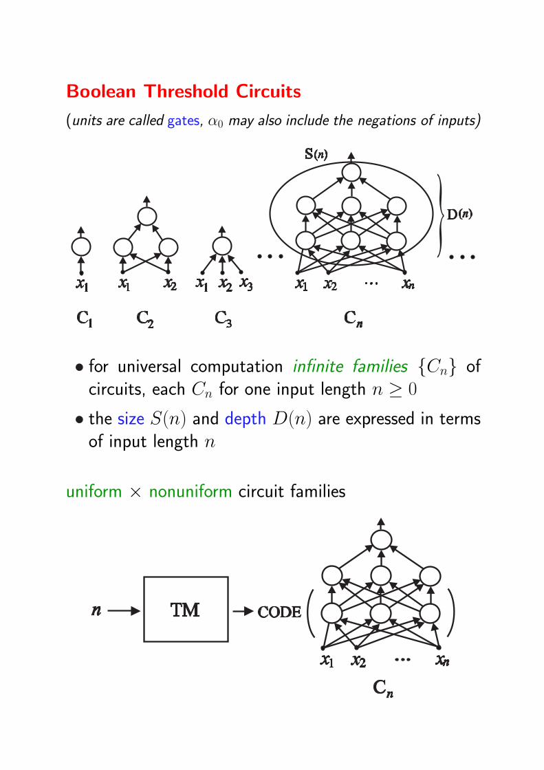
Boolean Threshold Circuits
(units are called gates, α0 may also include the negations of inputs)
• for universal computation infinite families Cn ofcircuits, each Cn for one input length n ≥ 0
• the size S(n) and depth D(n) are expressed in termsof input length n
uniform × nonuniform circuit families

A Taxonomy of Neural Network Models
1. Perceptron
Discrete Time
Deterministic Computation
(a) Single Perceptron
(b) Feedforward Architecture
i. Binary State ←−ii. Analog State
(c) Recurrent Architecture
i. Finite Size
A. Asymmetric Weights
B. Symmetric Weights
ii. Infinite Families of Networks
2. Probabilistic Computation
(a) Feedforward Architecture
(b) Recurrent Architecture
3. Continuous Time
4. RBF Unit
5. Winner-Take-All Unit
6. Spiking Neuron

1.b.i Binary-State Feedforward Networks:
computational universality: any vector Booleanfunction
f : 0, 1n −→ 0, 1mcan be implemented using 4-layer perceptron network with
Θ
(√m2n
n− log m
)neurons (Lupanov,1961)
lower bound: most functions require this network size(Horne,Hush,1994) and Ω(m2n/(n− log m)) connections(Cover,1968) even for unbounded depth
−→ (nonuniform) infinite families of threshold circuitswith exponentially many gates are capable of computingany I/O mapping in constant parallel time
polynomial weights: (each weight only O(log n) bits)exponential weights can constructively be replaced withpolynomial weights (in terms of input length) by increas-ing the depth by one layer while only a polynomial depth-independent increase in the network size is needed(Goldmann,Karpinski,1998)
N(s, d, wi = O(nn)) 7−→ N ′(O(sc1), d+1, wi = O(nc2))
−→ polynomial weights can be assumed in multi-layeredperceptron networks if one extra parallel computationalstep is granted

positive weights: at the cost of doubling the size(Hajnal et al.,1993)
N(s, d) 7−→ N ′(2s, d, wi ≥ 0)
unbounded fan-in:(fan-in is the maximum number of inputs to a single unit)
conventional circuit technology with bounded fan-in
× the dense interconnection of neurons
in feedforward networks yields a speed-up factor ofO(log log n) (i.e. the depth is reduced by this factor)at the cost of squaring the network size as compared tothe classical circuits with fan-in 2 (Chandra et al.,1984)
N(s, d, fan-in ≤ 2) 7−→ N ′(
O(s2) ,d
log log n
)
polynomial size & constant depth:
TC0d (d ≥ 1) is the class of all functions computable by
polynomial-size and polynomial-weight threshold circuitsof depth d (LT d × LTd for unbounded weights)
−→ a possible TC0 hierarchy , TC0 =⋃
d≥1 TC0d
TC01 ⊆ TC0
2 ⊆ TC03 ⊆ · · ·
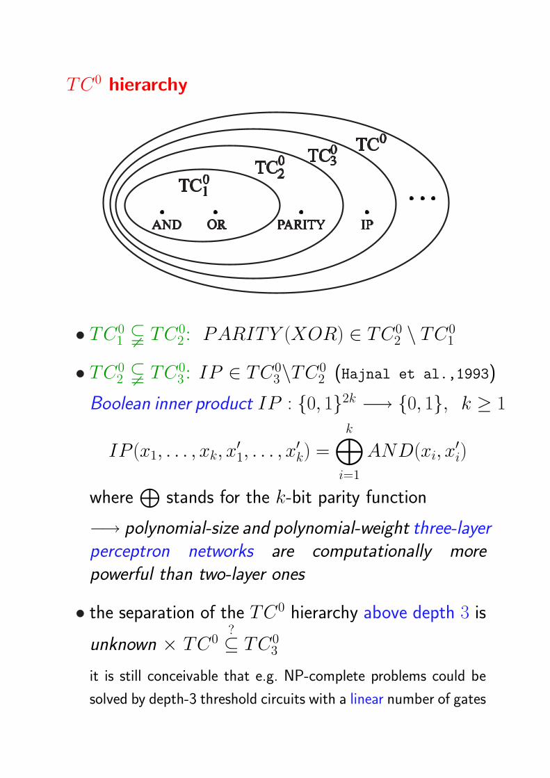
TC0 hierarchy
• TC01 $ TC0
2 : PARITY (XOR) ∈ TC02 \ TC0
1
• TC02 $ TC0
3 : IP ∈ TC03\TC0
2 (Hajnal et al.,1993)
Boolean inner product IP : 0, 12k −→ 0, 1, k ≥ 1
IP (x1, . . . , xk, x′1, . . . , x
′k) =
k⊕i=1
AND(xi, x′i)
where⊕
stands for the k-bit parity function
−→ polynomial-size and polynomial-weight three-layerperceptron networks are computationally morepowerful than two-layer ones
• the separation of the TC0 hierarchy above depth 3 is
unknown × TC0?⊆ TC0
3
it is still conceivable that e.g. NP-complete problems could be
solved by depth-3 threshold circuits with a linear number of gates
symmetric Boolean functions:
• the output value depends only on the number of 1swithin the input, e.g. AND, OR, PARITY
• any symmetric function f : 0, 1n −→ 0, 1 canbe implemented by a polynomial-weight depth-3threshold circuit of size O(
√n) (Siu et al.,1991)
lower bound: Ω(√
n/ log n) gates even for unboundeddepth and weights; Ω(
√n) for depth 2 (O’Neil,1971)
× PARITY 6∈ AC0, i.e. the parity cannot be com-puted by polynomial-size constant-depth AND-ORcircuits (Furst et al.,1984)
−→ perceptron networks are more efficient thanAND-OR circuits
• conjecture AC0?⊆ TC0
3 : AC0 functions are com-putable by depth-3 threshold circuits of subexponen-tial size nlogc n, for some constant c (Allender,1989)
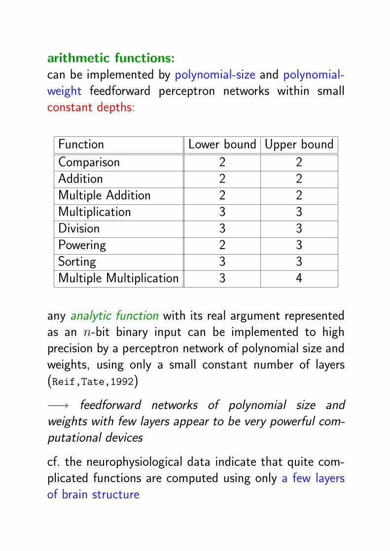
arithmetic functions:can be implemented by polynomial-size and polynomial-weight feedforward perceptron networks within smallconstant depths:
Function Lower bound Upper bound
Comparison 2 2Addition 2 2Multiple Addition 2 2Multiplication 3 3Division 3 3Powering 2 3Sorting 3 3Multiple Multiplication 3 4
any analytic function with its real argument representedas an n-bit binary input can be implemented to highprecision by a perceptron network of polynomial size andweights, using only a small constant number of layers(Reif,Tate,1992)
−→ feedforward networks of polynomial size andweights with few layers appear to be very powerful com-putational devices
cf. the neurophysiological data indicate that quite com-plicated functions are computed using only a few layersof brain structure
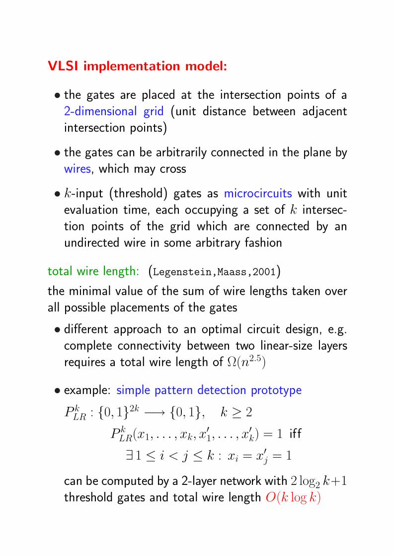
VLSI implementation model:
• the gates are placed at the intersection points of a2-dimensional grid (unit distance between adjacentintersection points)
• the gates can be arbitrarily connected in the plane bywires, which may cross
• k-input (threshold) gates as microcircuits with unitevaluation time, each occupying a set of k intersec-tion points of the grid which are connected by anundirected wire in some arbitrary fashion
total wire length: (Legenstein,Maass,2001)
the minimal value of the sum of wire lengths taken overall possible placements of the gates
• different approach to an optimal circuit design, e.g.complete connectivity between two linear-size layersrequires a total wire length of Ω(n2.5)
• example: simple pattern detection prototype
P kLR : 0, 12k −→ 0, 1, k ≥ 2
P kLR(x1, . . . , xk, x
′1, . . . , x
′k) = 1 iff
∃ 1 ≤ i < j ≤ k : xi = x′j = 1
can be computed by a 2-layer network with 2 log2 k+1threshold gates and total wire length O(k log k)
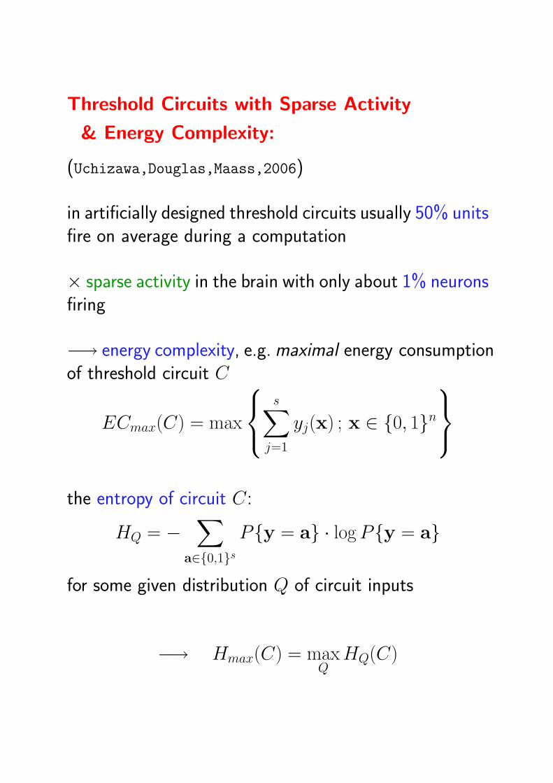
Threshold Circuits with Sparse Activity
& Energy Complexity:
(Uchizawa,Douglas,Maass,2006)
in artificially designed threshold circuits usually 50% unitsfire on average during a computation
× sparse activity in the brain with only about 1% neuronsfiring
−→ energy complexity, e.g. maximal energy consumptionof threshold circuit C
ECmax(C) = max
s∑j=1
yj(x) ; x ∈ 0, 1n
the entropy of circuit C:
HQ = −∑
a∈0,1sPy = a · log Py = a
for some given distribution Q of circuit inputs
−→ Hmax(C) = maxQ
HQ(C)
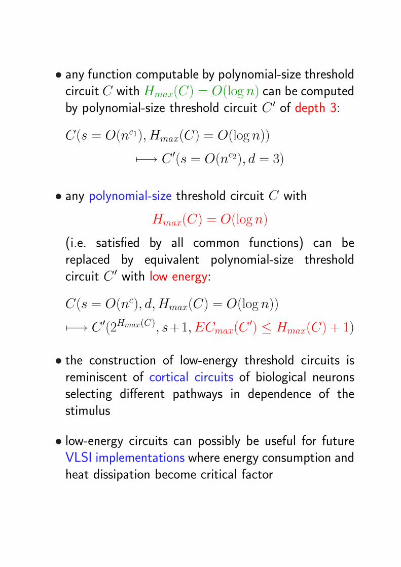
• any function computable by polynomial-size thresholdcircuit C with Hmax(C) = O(log n) can be computedby polynomial-size threshold circuit C ′ of depth 3:
C(s = O(nc1), Hmax(C) = O(log n))
7−→ C ′(s = O(nc2), d = 3)
• any polynomial-size threshold circuit C with
Hmax(C) = O(log n)
(i.e. satisfied by all common functions) can bereplaced by equivalent polynomial-size thresholdcircuit C ′ with low energy:
C(s = O(nc), d, Hmax(C) = O(log n))
7−→ C ′(2Hmax(C), s+1, ECmax(C′) ≤ Hmax(C) + 1)
• the construction of low-energy threshold circuits isreminiscent of cortical circuits of biological neuronsselecting different pathways in dependence of thestimulus
• low-energy circuits can possibly be useful for futureVLSI implementations where energy consumption andheat dissipation become critical factor
A Taxonomy of Neural Network Models
1. Perceptron
Discrete Time
Deterministic Computation
(a) Single Perceptron
(b) Feedforward Architecture
i. Binary State
ii. Analog State ←−(c) Recurrent Architecture
i. Finite Size
A. Asymmetric Weights
B. Symmetric Weights
ii. Infinite Families of Networks
2. Probabilistic Computation
(a) Feedforward Architecture
(b) Recurrent Architecture
3. Continuous Time
4. RBF Unit
5. Winner-Take-All Unit
6. Spiking Neuron
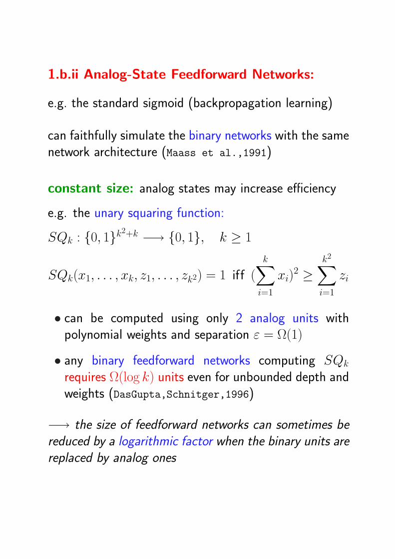
1.b.ii Analog-State Feedforward Networks:
e.g. the standard sigmoid (backpropagation learning)
can faithfully simulate the binary networks with the samenetwork architecture (Maass et al.,1991)
constant size: analog states may increase efficiency
e.g. the unary squaring function:
SQk : 0, 1k2+k −→ 0, 1, k ≥ 1
SQk(x1, . . . , xk, z1, . . . , zk2) = 1 iff (
k∑i=1
xi)2 ≥
k2∑i=1
zi
• can be computed using only 2 analog units withpolynomial weights and separation ε = Ω(1)
• any binary feedforward networks computing SQk
requires Ω(log k) units even for unbounded depth andweights (DasGupta,Schnitger,1996)
−→ the size of feedforward networks can sometimes bereduced by a logarithmic factor when the binary units arereplaced by analog ones
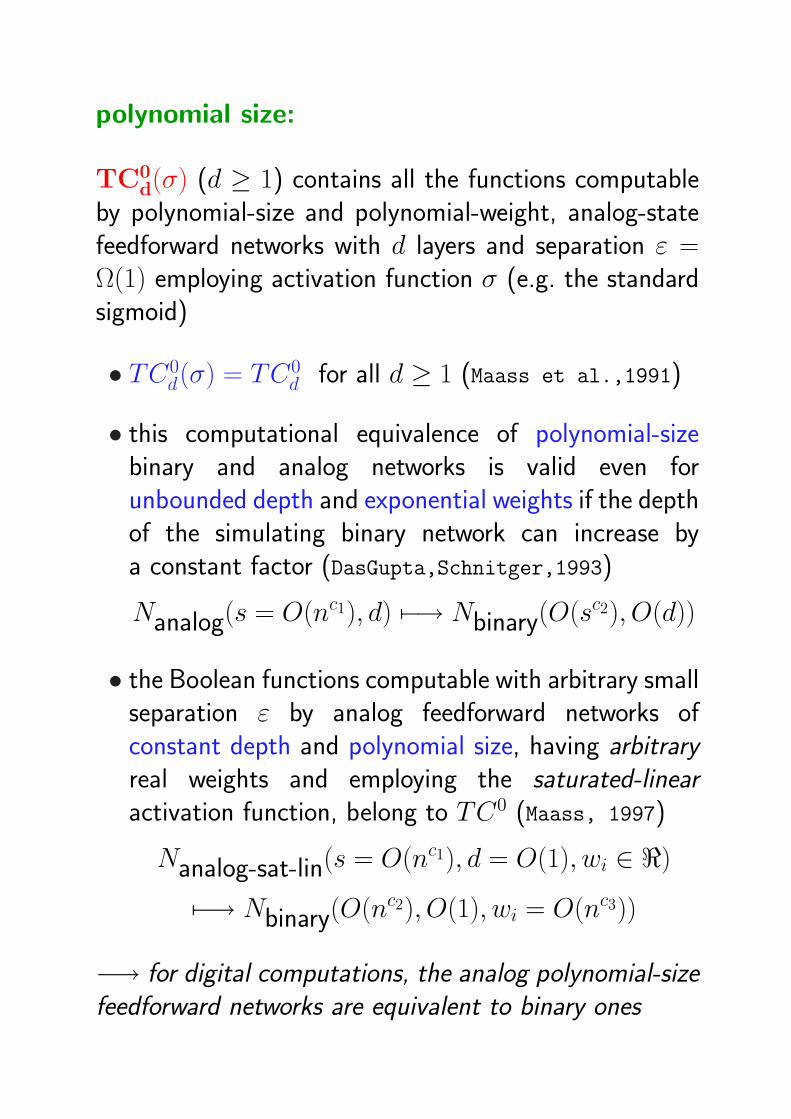
polynomial size:
TC0d(σ) (d ≥ 1) contains all the functions computable
by polynomial-size and polynomial-weight, analog-statefeedforward networks with d layers and separation ε =Ω(1) employing activation function σ (e.g. the standardsigmoid)
• TC0d(σ) = TC0
d for all d ≥ 1 (Maass et al.,1991)
• this computational equivalence of polynomial-sizebinary and analog networks is valid even forunbounded depth and exponential weights if the depthof the simulating binary network can increase bya constant factor (DasGupta,Schnitger,1993)
Nanalog(s = O(nc1), d) 7−→ Nbinary(O(sc2), O(d))
• the Boolean functions computable with arbitrary smallseparation ε by analog feedforward networks ofconstant depth and polynomial size, having arbitraryreal weights and employing the saturated-linearactivation function, belong to TC0 (Maass, 1997)
Nanalog-sat-lin(s = O(nc1), d = O(1), wi ∈ <)
7−→ Nbinary(O(nc2), O(1), wi = O(nc3))
−→ for digital computations, the analog polynomial-sizefeedforward networks are equivalent to binary ones
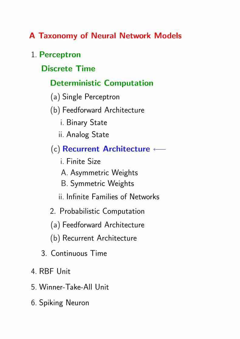
A Taxonomy of Neural Network Models
1. Perceptron
Discrete Time
Deterministic Computation
(a) Single Perceptron
(b) Feedforward Architecture
i. Binary State
ii. Analog State
(c) Recurrent Architecture ←−i. Finite Size
A. Asymmetric Weights
B. Symmetric Weights
ii. Infinite Families of Networks
2. Probabilistic Computation
(a) Feedforward Architecture
(b) Recurrent Architecture
3. Continuous Time
4. RBF Unit
5. Winner-Take-All Unit
6. Spiking Neuron
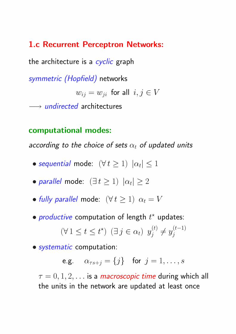
1.c Recurrent Perceptron Networks:
the architecture is a cyclic graph
symmetric (Hopfield) networks
wij = wji for all i, j ∈ V
−→ undirected architectures
computational modes:
according to the choice of sets αt of updated units
• sequential mode: (∀ t ≥ 1) |αt| ≤ 1
• parallel mode: (∃ t ≥ 1) |αt| ≥ 2
• fully parallel mode: (∀ t ≥ 1) αt = V
• productive computation of length t? updates:
(∀ 1 ≤ t ≤ t?) (∃ j ∈ αt) y(t)j 6= y
(t−1)j
• systematic computation:
e.g. ατs+j = j for j = 1, . . . , s
τ = 0, 1, 2, . . . is a macroscopic time during which allthe units in the network are updated at least once
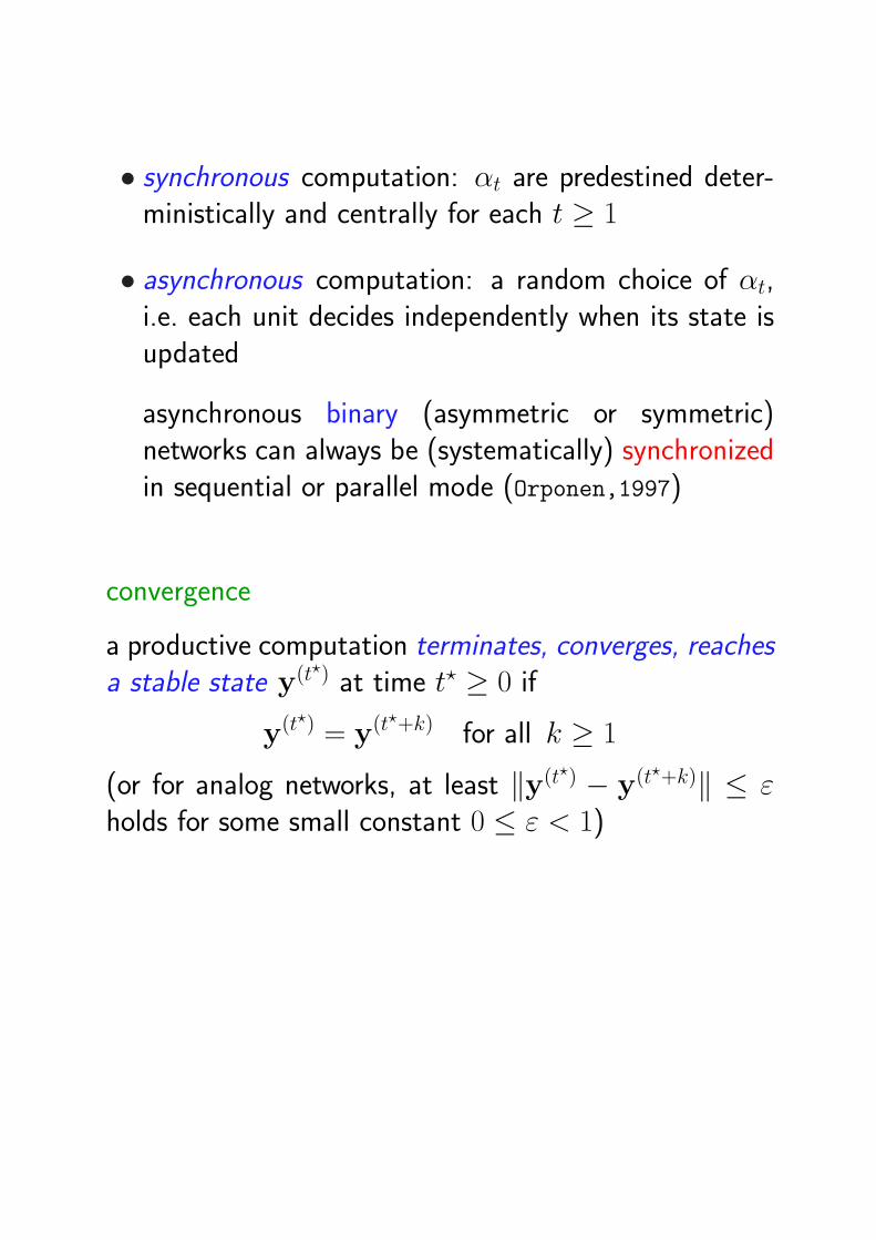
• synchronous computation: αt are predestined deter-ministically and centrally for each t ≥ 1
• asynchronous computation: a random choice of αt,i.e. each unit decides independently when its state isupdated
asynchronous binary (asymmetric or symmetric)networks can always be (systematically) synchronizedin sequential or parallel mode (Orponen,1997)
convergence
a productive computation terminates, converges, reachesa stable state y(t?) at time t? ≥ 0 if
y(t?) = y(t?+k) for all k ≥ 1
(or for analog networks, at least ‖y(t?) − y(t?+k)‖ ≤ εholds for some small constant 0 ≤ ε < 1)
A Taxonomy of Neural Network Models
1. Perceptron
Discrete Time
Deterministic Computation
(a) Single Perceptron
(b) Feedforward Architecture
i. Binary State
ii. Analog State
(c) Recurrent Architecture
i. Finite Size ←−A. Asymmetric Weights
B. Symmetric Weights
ii. Infinite Families of Networks
2. Probabilistic Computation
(a) Feedforward Architecture
(b) Recurrent Architecture
3. Continuous Time
4. RBF Unit
5. Winner-Take-All Unit
6. Spiking Neuron
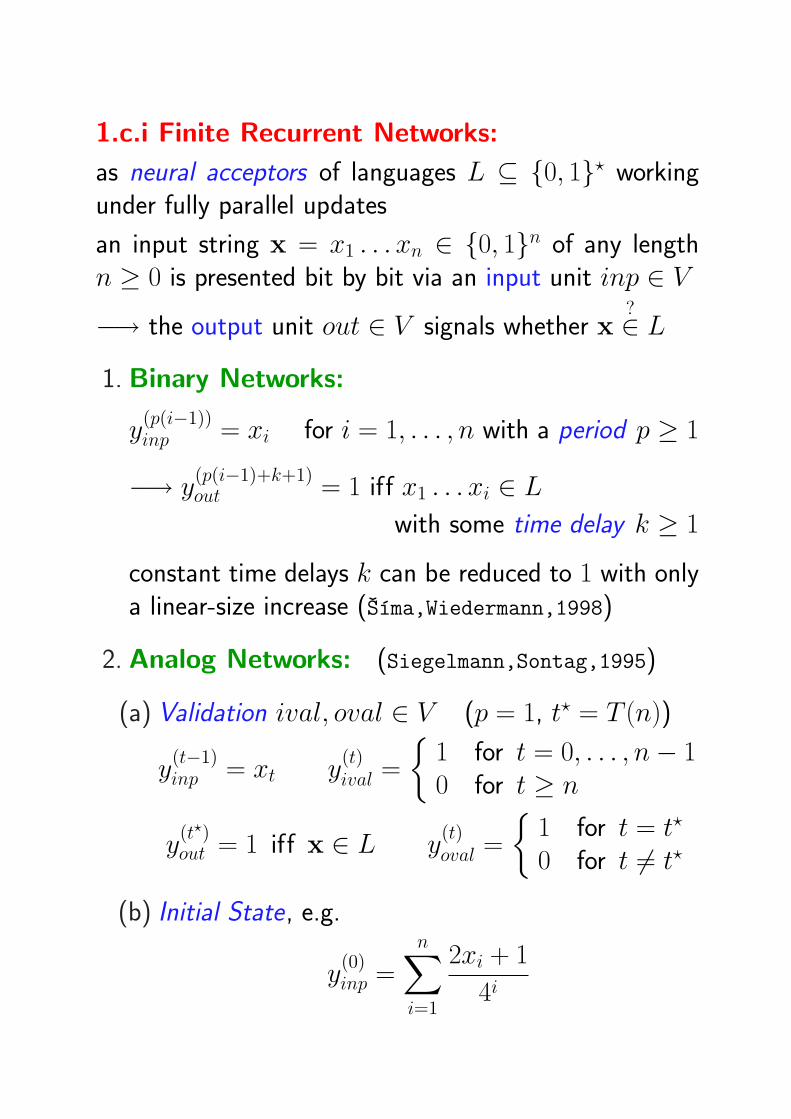
1.c.i Finite Recurrent Networks:
as neural acceptors of languages L ⊆ 0, 1? workingunder fully parallel updates
an input string x = x1 . . . xn ∈ 0, 1n of any lengthn ≥ 0 is presented bit by bit via an input unit inp ∈ V
−→ the output unit out ∈ V signals whether x?∈ L
1. Binary Networks:
y(p(i−1))inp = xi for i = 1, . . . , n with a period p ≥ 1
−→ y(p(i−1)+k+1)out = 1 iff x1 . . . xi ∈ L
with some time delay k ≥ 1
constant time delays k can be reduced to 1 with onlya linear-size increase (Sıma,Wiedermann,1998)
2. Analog Networks: (Siegelmann,Sontag,1995)
(a) Validation ival, oval ∈ V (p = 1, t? = T (n))
y(t−1)inp = xt y
(t)ival =
1 for t = 0, . . . , n− 10 for t ≥ n
y(t?)out = 1 iff x ∈ L y
(t)oval =
1 for t = t?
0 for t 6= t?
(b) Initial State, e.g.
y(0)inp =
n∑i=1
2xi + 1
4i
A Taxonomy of Neural Network Models
1. Perceptron
Discrete Time
Deterministic Computation
(a) Single Perceptron
(b) Feedforward Architecture
i. Binary State
ii. Analog State
(c) Recurrent Architecture
i. Finite Size
A. Asymmetric Weights ←−B. Symmetric Weights
ii. Infinite Families of Networks
2. Probabilistic Computation
(a) Feedforward Architecture
(b) Recurrent Architecture
3. Continuous Time
4. RBF Unit
5. Winner-Take-All Unit
6. Spiking Neuron
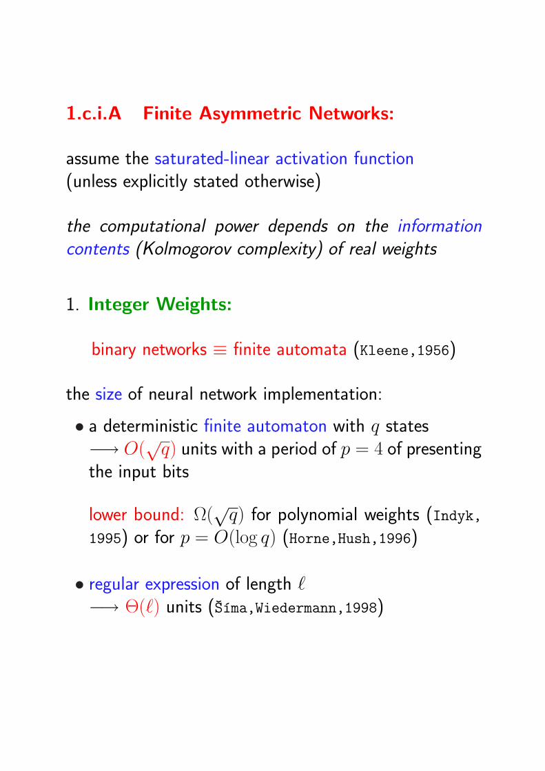
1.c.i.A Finite Asymmetric Networks:
assume the saturated-linear activation function(unless explicitly stated otherwise)
the computational power depends on the informationcontents (Kolmogorov complexity) of real weights
1. Integer Weights:
binary networks ≡ finite automata (Kleene,1956)
the size of neural network implementation:
• a deterministic finite automaton with q states−→ O(
√q) units with a period of p = 4 of presenting
the input bits
lower bound: Ω(√
q) for polynomial weights (Indyk,1995) or for p = O(log q) (Horne,Hush,1996)
• regular expression of length `−→ Θ(`) units (Sıma,Wiedermann,1998)

2. Rational Weights:
analog networks ≡ Turing machine
(step by step simulation)
−→ any function computable by a Turing machine intime T (n) can be computed by a fixed universal analognetwork of size:
• 886 units in time O(T (n)) (Siegelmann,Sontag,1995)
• 25 units in time O(n2T (n)) (Indyk,1995)
−→ polynomial-time computations by analog networkscorrespond to the complexity class P
Turing universality for more general classes of sigmoidactivation functions (Koiran,1996) including the stan-dard sigmoid (Kilian,Siegelmann,1996) but the knownsimulations require exponential time overhead per eachcomputational step
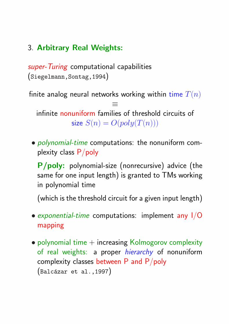
3. Arbitrary Real Weights:
super-Turing computational capabilities(Siegelmann,Sontag,1994)
finite analog neural networks working within time T (n)≡
infinite nonuniform families of threshold circuits ofsize S(n) = O(poly(T (n)))
• polynomial-time computations: the nonuniform com-plexity class P/poly
P/poly: polynomial-size (nonrecursive) advice (thesame for one input length) is granted to TMs workingin polynomial time
(which is the threshold circuit for a given input length)
• exponential-time computations: implement any I/Omapping
• polynomial time + increasing Kolmogorov complexityof real weights: a proper hierarchy of nonuniformcomplexity classes between P and P/poly(Balcazar et al.,1997)
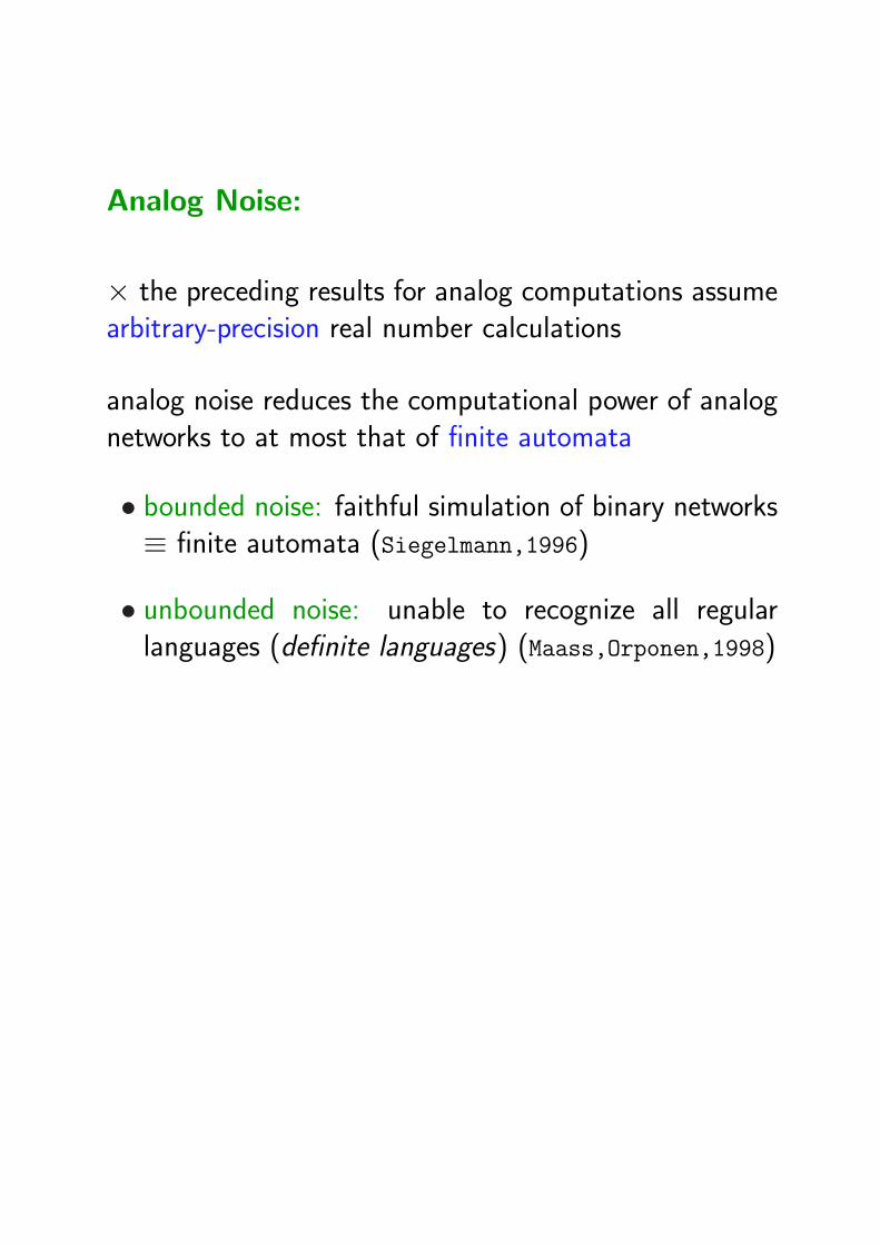
Analog Noise:
× the preceding results for analog computations assumearbitrary-precision real number calculations
analog noise reduces the computational power of analognetworks to at most that of finite automata
• bounded noise: faithful simulation of binary networks≡ finite automata (Siegelmann,1996)
• unbounded noise: unable to recognize all regularlanguages (definite languages) (Maass,Orponen,1998)
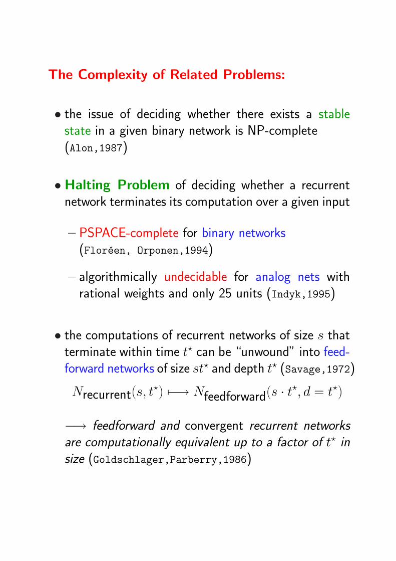
The Complexity of Related Problems:
• the issue of deciding whether there exists a stablestate in a given binary network is NP-complete(Alon,1987)
• Halting Problem of deciding whether a recurrentnetwork terminates its computation over a given input
– PSPACE-complete for binary networks(Floreen, Orponen,1994)
– algorithmically undecidable for analog nets withrational weights and only 25 units (Indyk,1995)
• the computations of recurrent networks of size s thatterminate within time t? can be “unwound” into feed-forward networks of size st? and depth t? (Savage,1972)
Nrecurrent(s, t?) 7−→ Nfeedforward(s · t?, d = t?)
−→ feedforward and convergent recurrent networksare computationally equivalent up to a factor of t? insize (Goldschlager,Parberry,1986)

A Taxonomy of Neural Network Models
1. Perceptron
Discrete Time
Deterministic Computation
(a) Single Perceptron
(b) Feedforward Architecture
i. Binary State
ii. Analog State
(c) Recurrent Architecture
i. Finite Size
A. Asymmetric Weights
B. Symmetric Weights ←−ii. Infinite Families of Networks
2. Probabilistic Computation
(a) Feedforward Architecture
(b) Recurrent Architecture
3. Continuous Time
4. RBF Unit
5. Winner-Take-All Unit
6. Spiking Neuron
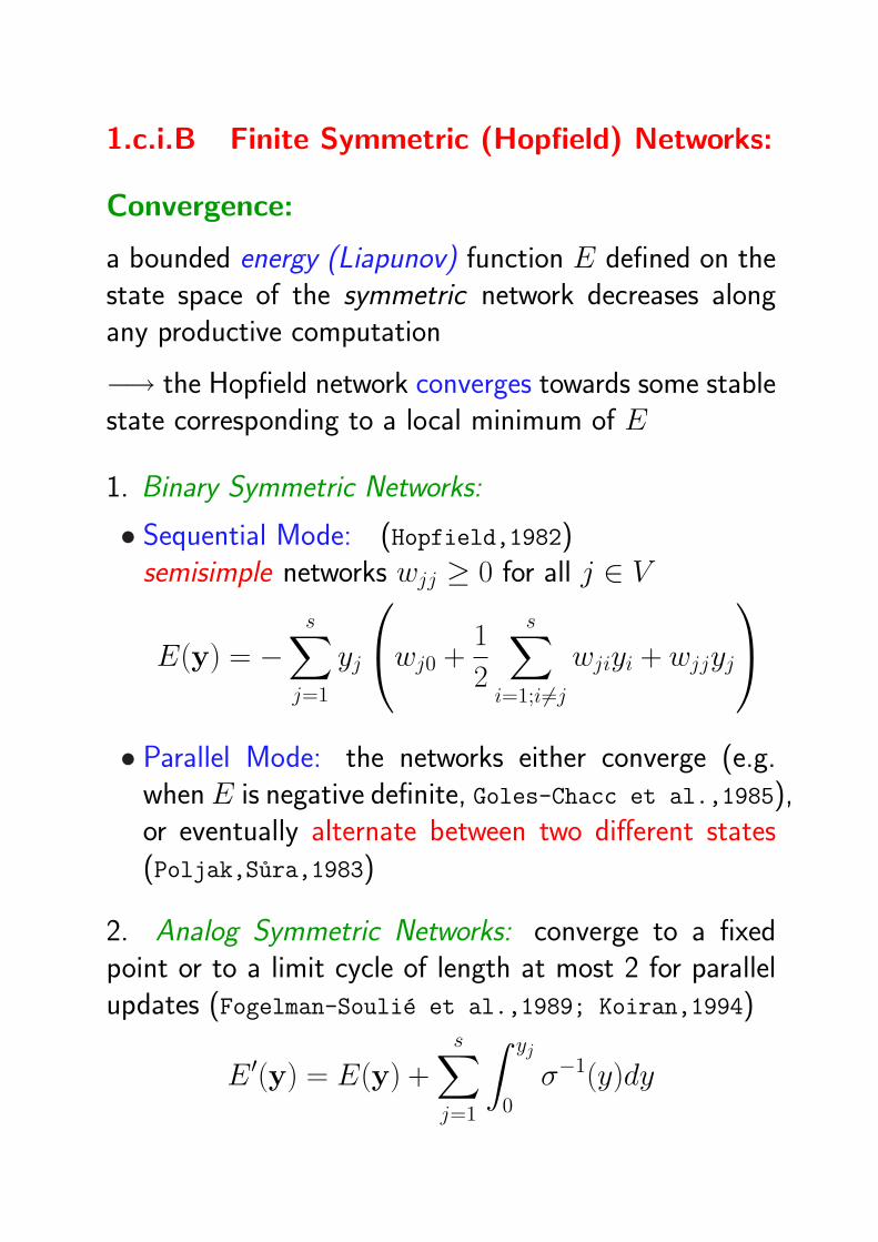
1.c.i.B Finite Symmetric (Hopfield) Networks:
Convergence:
a bounded energy (Liapunov) function E defined on thestate space of the symmetric network decreases alongany productive computation
−→ the Hopfield network converges towards some stablestate corresponding to a local minimum of E
1. Binary Symmetric Networks:
• Sequential Mode: (Hopfield,1982)semisimple networks wjj ≥ 0 for all j ∈ V
E(y) = −s∑
j=1
yj
wj0 +
1
2
s∑
i=1;i 6=j
wjiyi + wjjyj
• Parallel Mode: the networks either converge (e.g.when E is negative definite, Goles-Chacc et al.,1985),or eventually alternate between two different states(Poljak,Sura,1983)
2. Analog Symmetric Networks: converge to a fixedpoint or to a limit cycle of length at most 2 for parallelupdates (Fogelman-Soulie et al.,1989; Koiran,1994)
E ′(y) = E(y) +
s∑j=1
∫ yj
0
σ−1(y)dy
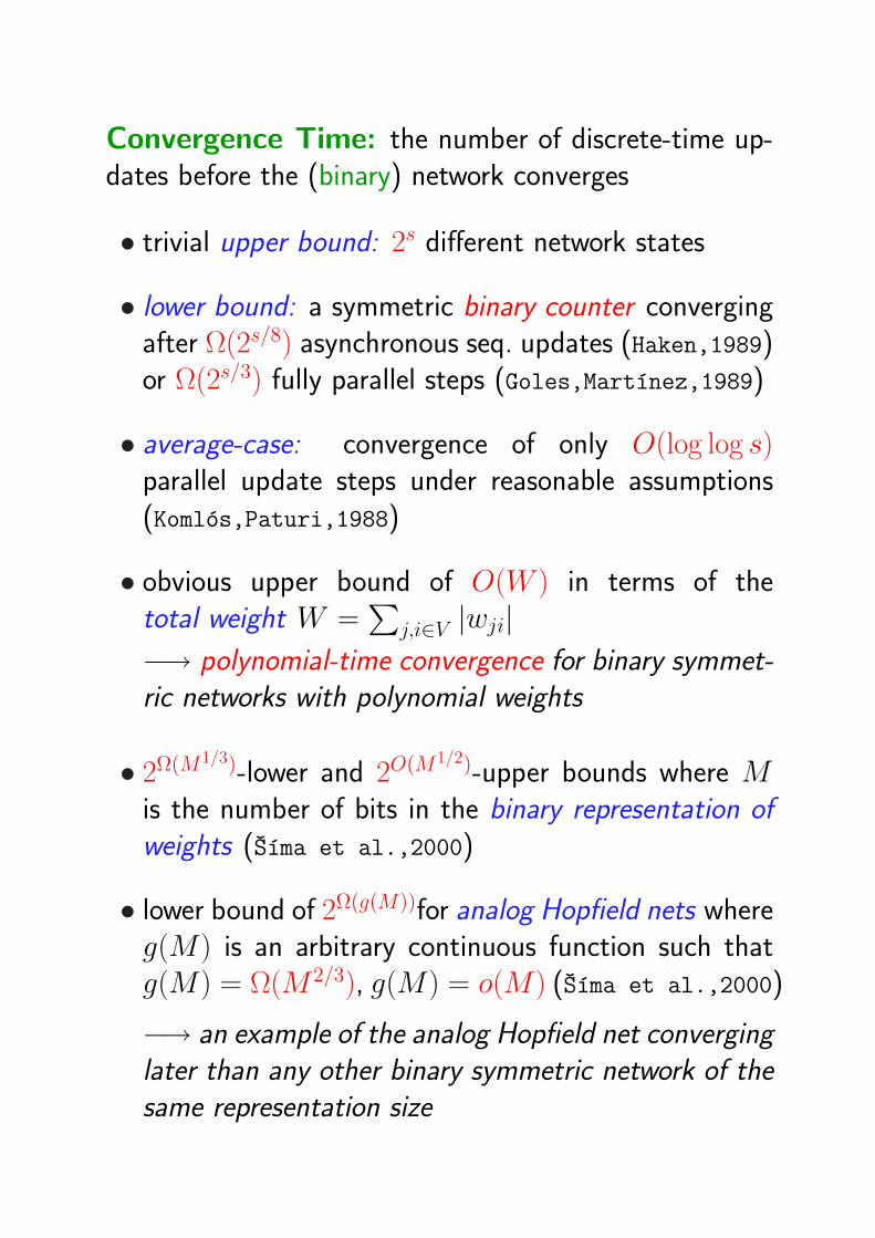
Convergence Time: the number of discrete-time up-dates before the (binary) network converges
• trivial upper bound: 2s different network states
• lower bound: a symmetric binary counter convergingafter Ω(2s/8) asynchronous seq. updates (Haken,1989)or Ω(2s/3) fully parallel steps (Goles,Martınez,1989)
• average-case: convergence of only O(log log s)parallel update steps under reasonable assumptions(Komlos,Paturi,1988)
• obvious upper bound of O(W ) in terms of thetotal weight W =
∑j,i∈V |wji|
−→ polynomial-time convergence for binary symmet-ric networks with polynomial weights
• 2Ω(M1/3)-lower and 2O(M1/2)-upper bounds where Mis the number of bits in the binary representation ofweights (Sıma et al.,2000)
• lower bound of 2Ω(g(M))for analog Hopfield nets whereg(M) is an arbitrary continuous function such thatg(M) = Ω(M 2/3), g(M) = o(M) (Sıma et al.,2000)
−→ an example of the analog Hopfield net converginglater than any other binary symmetric network of thesame representation size
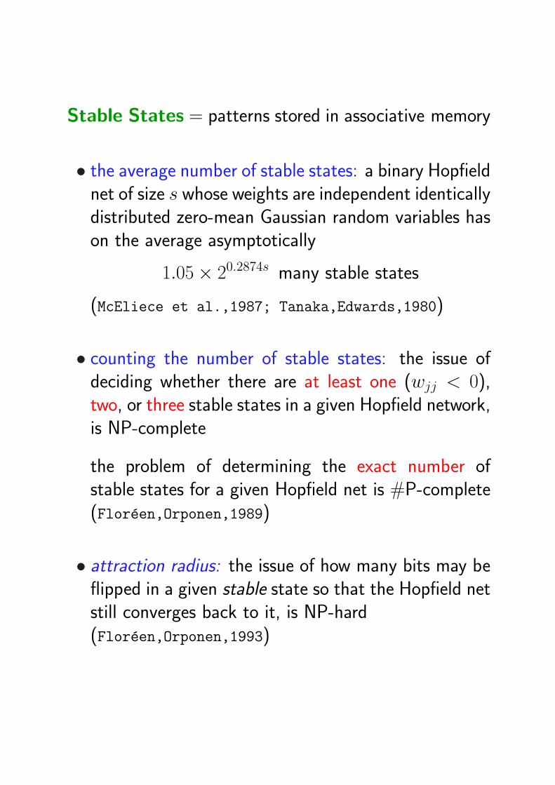
Stable States = patterns stored in associative memory
• the average number of stable states: a binary Hopfieldnet of size s whose weights are independent identicallydistributed zero-mean Gaussian random variables hason the average asymptotically
1.05× 20.2874s many stable states
(McEliece et al.,1987; Tanaka,Edwards,1980)
• counting the number of stable states: the issue ofdeciding whether there are at least one (wjj < 0),two, or three stable states in a given Hopfield network,is NP-complete
the problem of determining the exact number ofstable states for a given Hopfield net is #P-complete(Floreen,Orponen,1989)
• attraction radius: the issue of how many bits may beflipped in a given stable state so that the Hopfield netstill converges back to it, is NP-hard(Floreen,Orponen,1993)
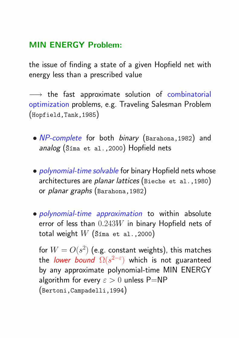
MIN ENERGY Problem:
the issue of finding a state of a given Hopfield net withenergy less than a prescribed value
−→ the fast approximate solution of combinatorialoptimization problems, e.g. Traveling Salesman Problem(Hopfield,Tank,1985)
• NP-complete for both binary (Barahona,1982) andanalog (Sıma et al.,2000) Hopfield nets
• polynomial-time solvable for binary Hopfield nets whosearchitectures are planar lattices (Bieche et al.,1980)or planar graphs (Barahona,1982)
• polynomial-time approximation to within absoluteerror of less than 0.243W in binary Hopfield nets oftotal weight W (Sıma et al.,2000)
for W = O(s2) (e.g. constant weights), this matchesthe lower bound Ω(s2−ε) which is not guaranteedby any approximate polynomial-time MIN ENERGYalgorithm for every ε > 0 unless P=NP(Bertoni,Campadelli,1994)
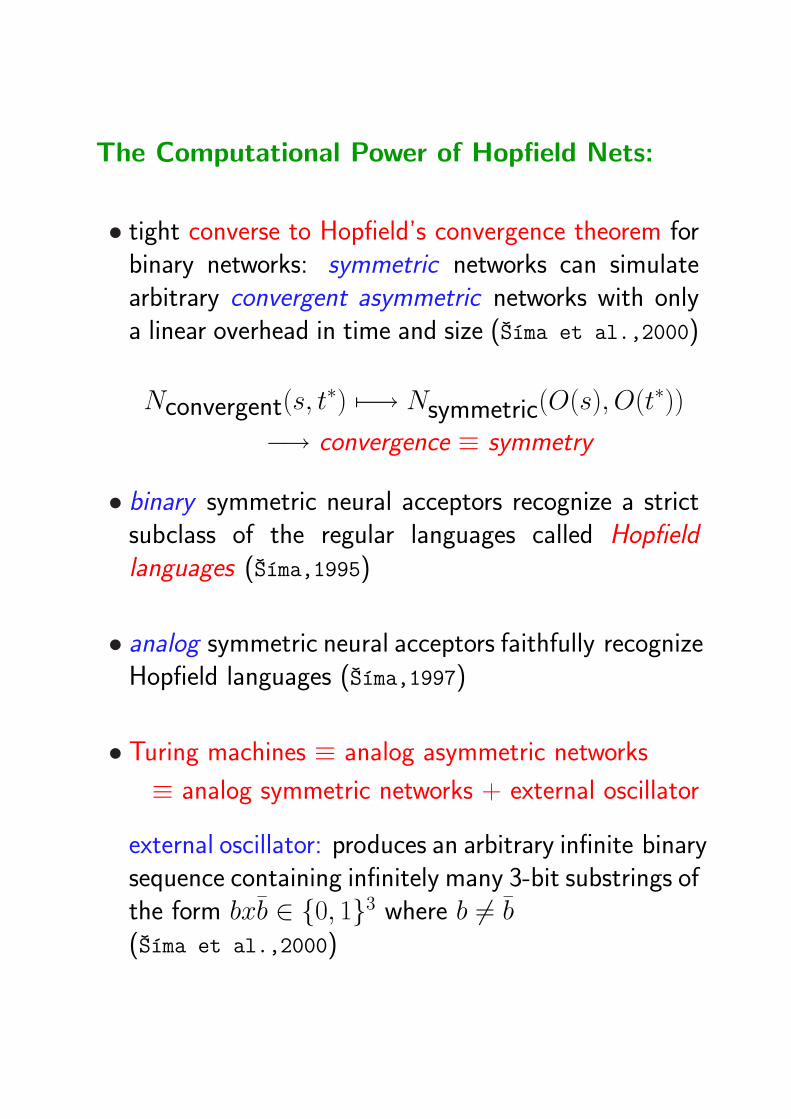
The Computational Power of Hopfield Nets:
• tight converse to Hopfield’s convergence theorem forbinary networks: symmetric networks can simulatearbitrary convergent asymmetric networks with onlya linear overhead in time and size (Sıma et al.,2000)
Nconvergent(s, t∗) 7−→ Nsymmetric(O(s), O(t∗))
−→ convergence ≡ symmetry
• binary symmetric neural acceptors recognize a strictsubclass of the regular languages called Hopfieldlanguages (Sıma,1995)
• analog symmetric neural acceptors faithfully recognizeHopfield languages (Sıma,1997)
• Turing machines ≡ analog asymmetric networks
≡ analog symmetric networks + external oscillator
external oscillator: produces an arbitrary infinite binarysequence containing infinitely many 3-bit substrings ofthe form bxb ∈ 0, 13 where b 6= b(Sıma et al.,2000)
A Taxonomy of Neural Network Models
1. Perceptron
Discrete Time
Deterministic Computation
(a) Single Perceptron
(b) Feedforward Architecture
i. Binary State
ii. Analog State
(c) Recurrent Architecture
i. Finite Size
A. Asymmetric Weights
B. Symmetric Weights
ii. Infinite Families of Networks ←−2. Probabilistic Computation
(a) Feedforward Architecture
(b) Recurrent Architecture
3. Continuous Time
4. RBF Unit
5. Winner-Take-All Unit
6. Spiking Neuron
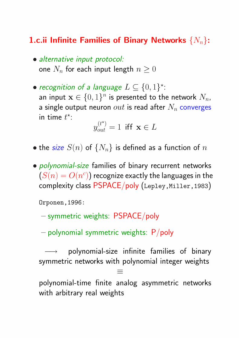
1.c.ii Infinite Families of Binary Networks Nn:
• alternative input protocol:one Nn for each input length n ≥ 0
• recognition of a language L ⊆ 0, 1?:an input x ∈ 0, 1n is presented to the network Nn,a single output neuron out is read after Nn convergesin time t?:
y(t?)out = 1 iff x ∈ L
• the size S(n) of Nn is defined as a function of n
• polynomial-size families of binary recurrent networks(S(n) = O(nc)) recognize exactly the languages in thecomplexity class PSPACE/poly (Lepley,Miller,1983)
Orponen,1996:
– symmetric weights: PSPACE/poly
– polynomial symmetric weights: P/poly
−→ polynomial-size infinite families of binarysymmetric networks with polynomial integer weights
≡polynomial-time finite analog asymmetric networkswith arbitrary real weights
A Taxonomy of Neural Network Models
1. Perceptron
Discrete Time
Deterministic Computation
(a) Single Perceptron
(b) Feedforward Architecture
i. Binary State
ii. Analog State
(c) Recurrent Architecture
i. Finite Size
A. Asymmetric Weights
B. Symmetric Weights
ii. Infinite Families of Networks
2. Probabilistic Computation ←−(a) Feedforward Architecture
(b) Recurrent Architecture
3. Continuous Time
4. RBF Unit
5. Winner-Take-All Unit
6. Spiking Neuron
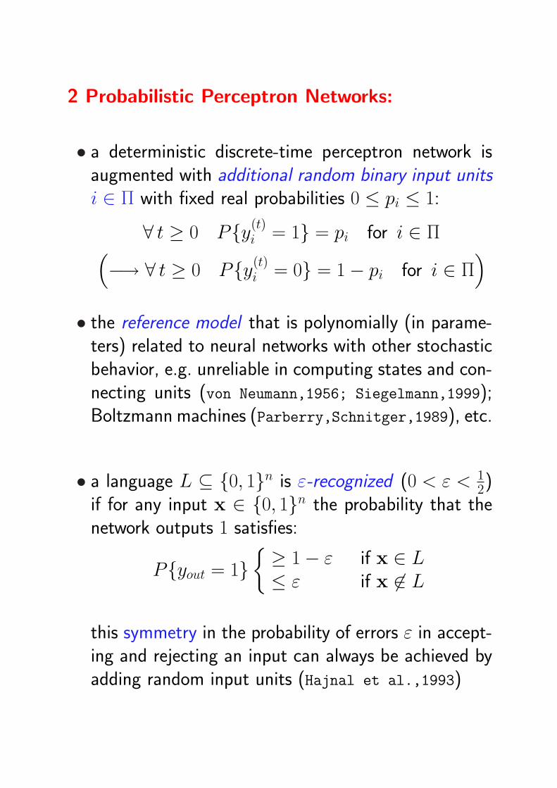
2 Probabilistic Perceptron Networks:
• a deterministic discrete-time perceptron network isaugmented with additional random binary input unitsi ∈ Π with fixed real probabilities 0 ≤ pi ≤ 1:
∀ t ≥ 0 Py(t)i = 1 = pi for i ∈ Π(
−→ ∀ t ≥ 0 Py(t)i = 0 = 1− pi for i ∈ Π
)
• the reference model that is polynomially (in parame-ters) related to neural networks with other stochasticbehavior, e.g. unreliable in computing states and con-necting units (von Neumann,1956; Siegelmann,1999);Boltzmann machines (Parberry,Schnitger,1989), etc.
• a language L ⊆ 0, 1n is ε-recognized (0 < ε < 12)
if for any input x ∈ 0, 1n the probability that thenetwork outputs 1 satisfies:
Pyout = 1 ≥ 1− ε if x ∈ L≤ ε if x 6∈ L
this symmetry in the probability of errors ε in accept-ing and rejecting an input can always be achieved byadding random input units (Hajnal et al.,1993)
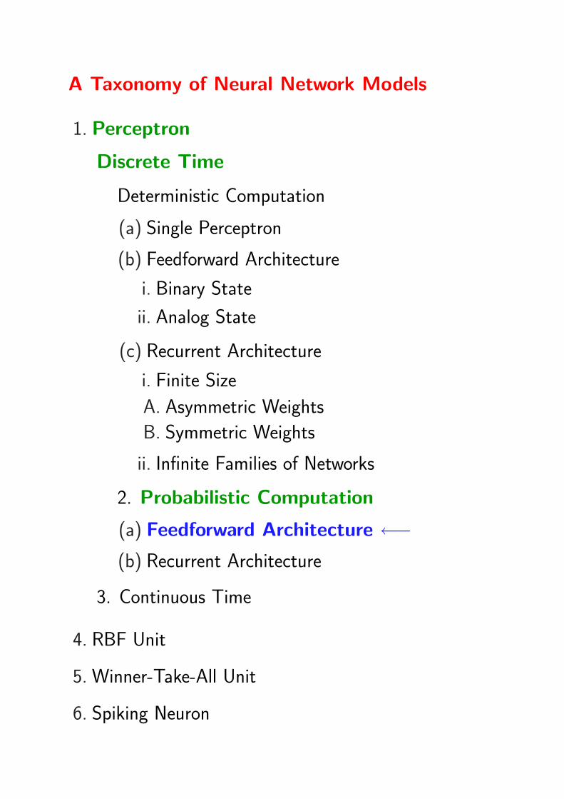
A Taxonomy of Neural Network Models
1. Perceptron
Discrete Time
Deterministic Computation
(a) Single Perceptron
(b) Feedforward Architecture
i. Binary State
ii. Analog State
(c) Recurrent Architecture
i. Finite Size
A. Asymmetric Weights
B. Symmetric Weights
ii. Infinite Families of Networks
2. Probabilistic Computation
(a) Feedforward Architecture ←−(b) Recurrent Architecture
3. Continuous Time
4. RBF Unit
5. Winner-Take-All Unit
6. Spiking Neuron
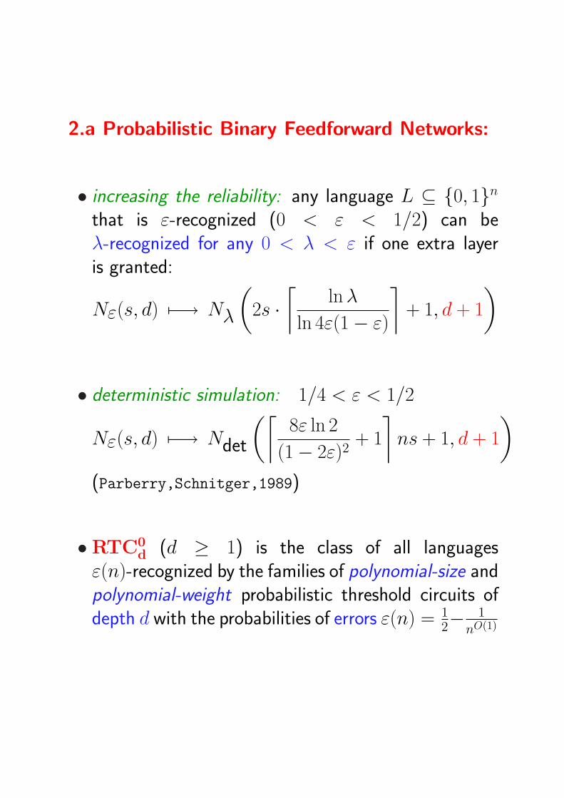
2.a Probabilistic Binary Feedforward Networks:
• increasing the reliability: any language L ⊆ 0, 1nthat is ε-recognized (0 < ε < 1/2) can beλ-recognized for any 0 < λ < ε if one extra layeris granted:
Nε(s, d) 7−→ Nλ
(2s ·
⌈ln λ
ln 4ε(1− ε)
⌉+ 1, d + 1
)
• deterministic simulation: 1/4 < ε < 1/2
Nε(s, d) 7−→ Ndet
(⌈8ε ln 2
(1− 2ε)2+ 1
⌉ns + 1, d + 1
)
(Parberry,Schnitger,1989)
•RTC0d (d ≥ 1) is the class of all languages
ε(n)-recognized by the families of polynomial-size andpolynomial-weight probabilistic threshold circuits ofdepth d with the probabilities of errors ε(n) = 1
2− 1nO(1)
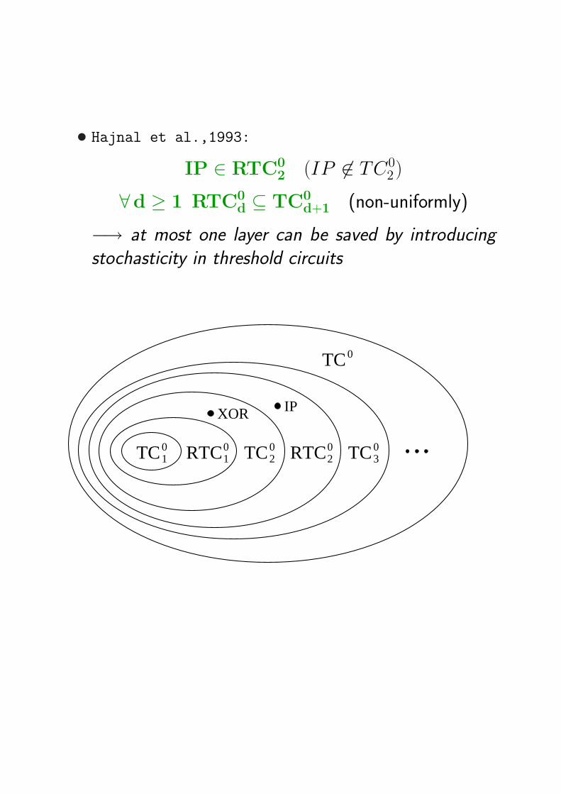
• Hajnal et al.,1993:
IP ∈ RTC02 (IP 6∈ TC0
2)
∀d ≥ 1 RTC0d ⊆ TC0
d+1 (non-uniformly)
−→ at most one layer can be saved by introducingstochasticity in threshold circuits
RTC10
XOR IP
TC20
TC0
TC10 TC0
3RTC02
A Taxonomy of Neural Network Models
1. Perceptron
Discrete Time
Deterministic Computation
(a) Single Perceptron
(b) Feedforward Architecture
i. Binary State
ii. Analog State
(c) Recurrent Architecture
i. Finite Size
A. Asymmetric Weights
B. Symmetric Weights
ii. Infinite Families of Networks
2. Probabilistic Computation
(a) Feedforward Architecture
(b) Recurrent Architecture ←−3. Continuous Time
4. RBF Unit
5. Winner-Take-All Unit
6. Spiking Neuron
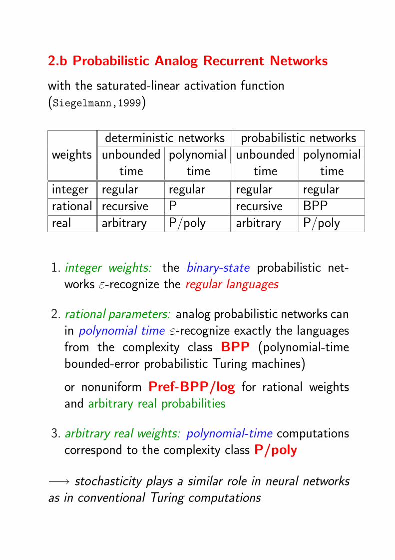
2.b Probabilistic Analog Recurrent Networks
with the saturated-linear activation function(Siegelmann,1999)
deterministic networks probabilistic networksweights unbounded polynomial unbounded polynomial
time time time time
integer regular regular regular regularrational recursive P recursive BPPreal arbitrary P/poly arbitrary P/poly
1. integer weights: the binary-state probabilistic net-works ε-recognize the regular languages
2. rational parameters: analog probabilistic networks canin polynomial time ε-recognize exactly the languagesfrom the complexity class BPP (polynomial-timebounded-error probabilistic Turing machines)
or nonuniform Pref-BPP/log for rational weightsand arbitrary real probabilities
3. arbitrary real weights: polynomial-time computationscorrespond to the complexity class P/poly
−→ stochasticity plays a similar role in neural networksas in conventional Turing computations
A Taxonomy of Neural Network Models
1. Perceptron
Discrete Time
Deterministic Computation
(a) Single Perceptron
(b) Feedforward Architecture
i. Binary State
ii. Analog State
(c) Recurrent Architecture
i. Finite Size
A. Asymmetric Weights
B. Symmetric Weights
ii. Infinite Families of Networks
2. Probabilistic Computation
(a) Feedforward Architecture
(b) Recurrent Architecture
3. Continuous Time ←−
4. RBF Unit
5. Winner-Take-All Unit
6. Spiking Neuron
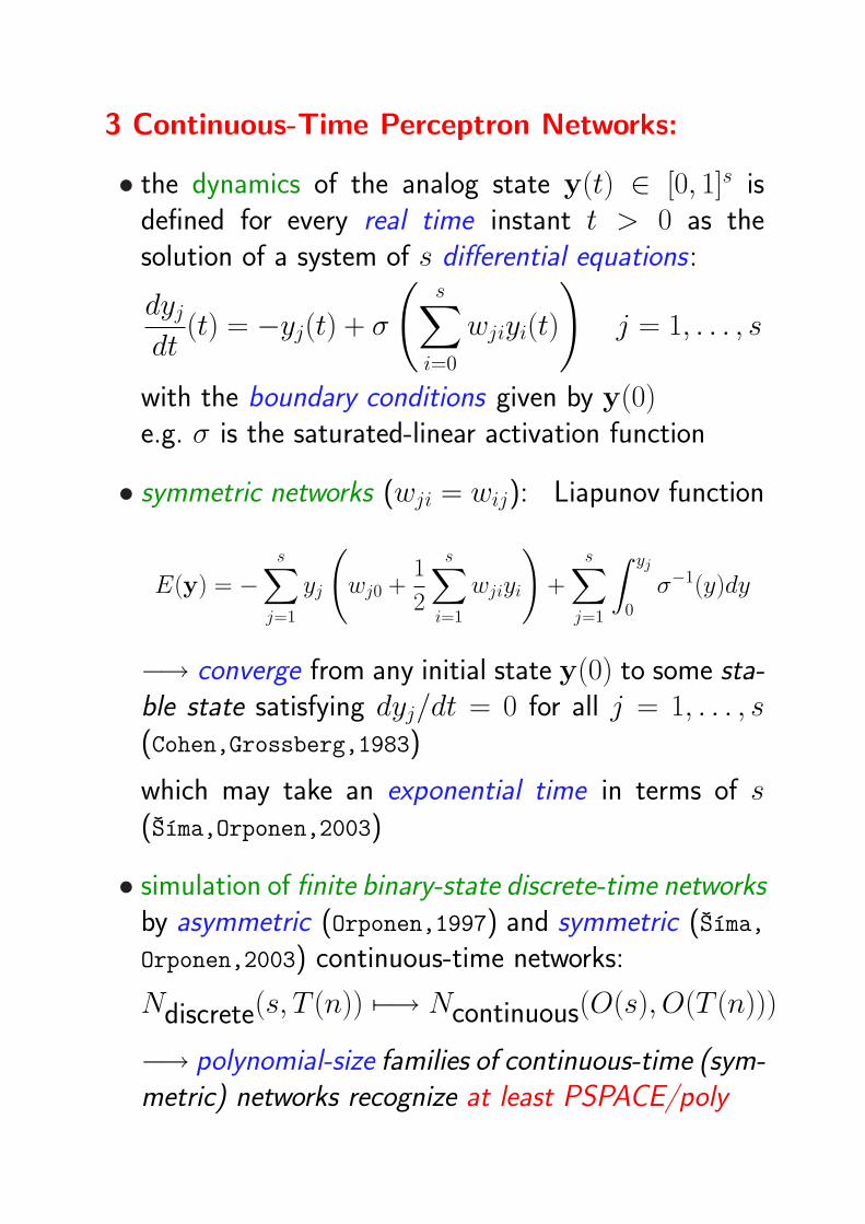
3 Continuous-Time Perceptron Networks:
• the dynamics of the analog state y(t) ∈ [0, 1]s isdefined for every real time instant t > 0 as thesolution of a system of s differential equations:
dyj
dt(t) = −yj(t) + σ
(s∑
i=0
wjiyi(t)
)j = 1, . . . , s
with the boundary conditions given by y(0)e.g. σ is the saturated-linear activation function
• symmetric networks (wji = wij): Liapunov function
E(y) = −s∑
j=1
yj
(wj0 +
1
2
s∑i=1
wjiyi
)+
s∑j=1
∫ yj
0
σ−1(y)dy
−→ converge from any initial state y(0) to some sta-ble state satisfying dyj/dt = 0 for all j = 1, . . . , s(Cohen,Grossberg,1983)
which may take an exponential time in terms of s(Sıma,Orponen,2003)
• simulation of finite binary-state discrete-time networksby asymmetric (Orponen,1997) and symmetric (Sıma,Orponen,2003) continuous-time networks:
Ndiscrete(s, T (n)) 7−→ Ncontinuous(O(s), O(T (n)))
−→ polynomial-size families of continuous-time (sym-metric) networks recognize at least PSPACE/poly
A Taxonomy of Neural Network Models
1. Perceptron
Discrete Time
Deterministic Computation
(a) Single Perceptron
(b) Feedforward Architecture
i. Binary State
ii. Analog State
(c) Recurrent Architecture
i. Finite Size
A. Asymmetric Weights
B. Symmetric Weights
ii. Infinite Families of Networks
2. Probabilistic Computation
(a) Feedforward Architecture
(b) Recurrent Architecture
3. Continuous Time
4. RBF Unit ←−5. Winner-Take-All Unit
6. Spiking Neuron
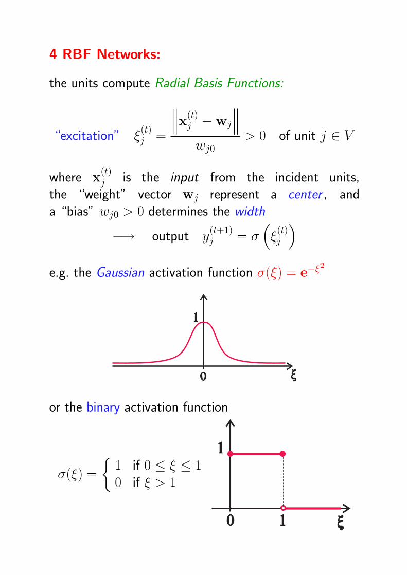
4 RBF Networks:
the units compute Radial Basis Functions:
“excitation” ξ(t)j =
∥∥∥x(t)j −wj
∥∥∥wj0
> 0 of unit j ∈ V
where x(t)j is the input from the incident units,
the “weight” vector wj represent a center , anda “bias” wj0 > 0 determines the width
−→ output y(t+1)j = σ
(ξ
(t)j
)
e.g. the Gaussian activation function σ(ξ) = e−ξ2
or the binary activation function
σ(ξ) =
1 if 0 ≤ ξ ≤ 10 if ξ > 1
the computational power of RBF networks:
• binary RBF units with the Euclidean norm computeexactly the Boolean linear threshold functions(Friedrichs,Schmitt,2005), i.e.
binary RBF unit ≡ perceptron
• digital computations using analog RBF unit: twodifferent analog states of RBF units represent thebinary values 0 and 1
• an analog RBF unit with the maximum norm canimplement the universal Boolean NAND gate overmultiple literals (input variables or their negations)
−→ a deterministic finite automaton with q states canbe simulated by a recurrent network with O(
√q log q)
RBF units in a robust way (Sorel,Sıma,2000)
• the Turing universality of finite RBF networks is stillan open problem
A Taxonomy of Neural Network Models
1. Perceptron
Discrete Time
Deterministic Computation
(a) Single Perceptron
(b) Feedforward Architecture
i. Binary State
ii. Analog State
(c) Recurrent Architecture
i. Finite Size
A. Asymmetric Weights
B. Symmetric Weights
ii. Infinite Families of Networks
2. Probabilistic Computation
(a) Feedforward Architecture
(b) Recurrent Architecture
3. Continuous Time
4. RBF Unit
5. Winner-Take-All Unit ←−6. Spiking Neuron

5 Winner-Take-All (WTA) Networks:
• competitive principle (e.g. Kohonen networks)
• efficient analog VLSI implementations
• the units compute k-WTAn : <n −→ 0, 1ndefined as
yj = 1 iff |i ; xi > xj, 1 ≤ i ≤ n| ≤ k − 1
e.g. a WTAn gate (k = 1) indicates which of then inputs has maximal value
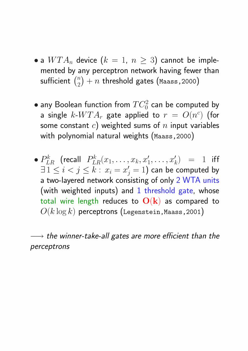
• a WTAn device (k = 1, n ≥ 3) cannot be imple-mented by any perceptron network having fewer thansufficient
(n2
)+ n threshold gates (Maass,2000)
• any Boolean function from TC20 can be computed by
a single k-WTAr gate applied to r = O(nc) (forsome constant c) weighted sums of n input variableswith polynomial natural weights (Maass,2000)
• P kLR (recall P k
LR(x1, . . . , xk, x′1, . . . , x
′k) = 1 iff
∃ 1 ≤ i < j ≤ k : xi = x′j = 1) can be computed bya two-layered network consisting of only 2 WTA units(with weighted inputs) and 1 threshold gate, whosetotal wire length reduces to O(k) as compared toO(k log k) perceptrons (Legenstein,Maass,2001)
−→ the winner-take-all gates are more efficient than theperceptrons
A Taxonomy of Neural Network Models
1. Perceptron
Discrete Time
Deterministic Computation
(a) Single Perceptron
(b) Feedforward Architecture
i. Binary State
ii. Analog State
(c) Recurrent Architecture
i. Finite Size
A. Asymmetric Weights
B. Symmetric Weights
ii. Infinite Families of Networks
2. Probabilistic Computation
(a) Feedforward Architecture
(b) Recurrent Architecture
3. Continuous Time
4. RBF Unit
5. Winner-Take-All Unit
6. Spiking Neuron ←−
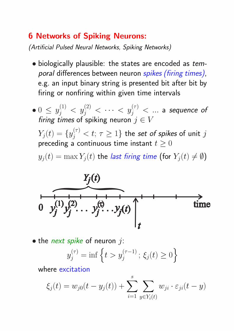
6 Networks of Spiking Neurons:
(Artificial Pulsed Neural Networks, Spiking Networks)
• biologically plausible: the states are encoded as tem-poral differences between neuron spikes (firing times),e.g. an input binary string is presented bit after bit byfiring or nonfiring within given time intervals
• 0 ≤ y(1)j < y
(2)j < · · · < y
(τ)j < ... a sequence of
firing times of spiking neuron j ∈ V
Yj(t) = y(τ)j < t; τ ≥ 1 the set of spikes of unit j
preceding a continuous time instant t ≥ 0
yj(t) = max Yj(t) the last firing time (for Yj(t) 6= ∅)
• the next spike of neuron j:
y(τ)j = inf
t > y
(τ−1)j ; ξj(t) ≥ 0
where excitation
ξj(t) = wj0(t− yj(t)) +
s∑i=1
∑
y∈Yi(t)
wji · εji(t− y)
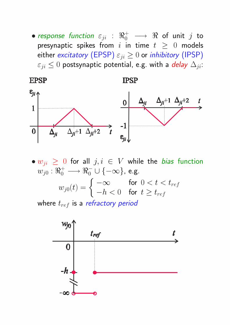
• response function εji : <+0 −→ < of unit j to
presynaptic spikes from i in time t ≥ 0 modelseither excitatory (EPSP) εji ≥ 0 or inhibitory (IPSP)εji ≤ 0 postsynaptic potential, e.g. with a delay ∆ji:
• wji ≥ 0 for all j, i ∈ V while the bias functionwj0 : <+
0 −→ <−0 ∪ −∞, e.g.
wj0(t) =
−∞ for 0 < t < tref−h < 0 for t ≥ tref
where tref is a refractory period
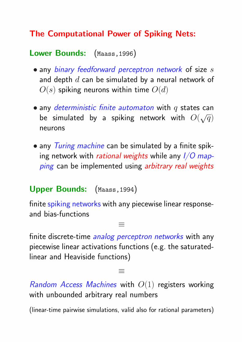
The Computational Power of Spiking Nets:
Lower Bounds: (Maass,1996)
• any binary feedforward perceptron network of size sand depth d can be simulated by a neural network ofO(s) spiking neurons within time O(d)
• any deterministic finite automaton with q states canbe simulated by a spiking network with O(
√q)
neurons
• any Turing machine can be simulated by a finite spik-ing network with rational weights while any I/O map-ping can be implemented using arbitrary real weights
Upper Bounds: (Maass,1994)
finite spiking networks with any piecewise linear response-and bias-functions
≡finite discrete-time analog perceptron networks with anypiecewise linear activations functions (e.g. the saturated-linear and Heaviside functions)
≡Random Access Machines with O(1) registers workingwith unbounded arbitrary real numbers
(linear-time pairwise simulations, valid also for rational parameters)
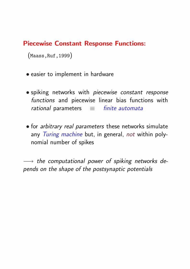
Piecewise Constant Response Functions:
(Maass,Ruf,1999)
• easier to implement in hardware
• spiking networks with piecewise constant responsefunctions and piecewise linear bias functions withrational parameters ≡ finite automata
• for arbitrary real parameters these networks simulateany Turing machine but, in general, not within poly-nomial number of spikes
−→ the computational power of spiking networks de-pends on the shape of the postsynaptic potentials
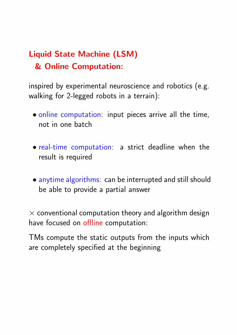
Liquid State Machine (LSM)
& Online Computation:
inspired by experimental neuroscience and robotics (e.g.walking for 2-legged robots in a terrain):
• online computation: input pieces arrive all the time,not in one batch
• real-time computation: a strict deadline when theresult is required
• anytime algorithms: can be interrupted and still shouldbe able to provide a partial answer
× conventional computation theory and algorithm designhave focused on offline computation:
TMs compute the static outputs from the inputs whichare completely specified at the beginning
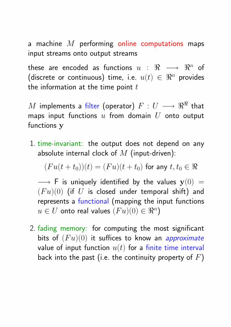
a machine M performing online computations mapsinput streams onto output streams
these are encoded as functions u : < −→ <n of(discrete or continuous) time, i.e. u(t) ∈ <n providesthe information at the time point t
M implements a filter (operator) F : U −→ << thatmaps input functions u from domain U onto outputfunctions y
1. time-invariant: the output does not depend on anyabsolute internal clock of M (input-driven):
(Fu(t + t0))(t) = (Fu)(t + t0) for any t, t0 ∈ <−→ F is uniquely identified by the values y(0) =(Fu)(0) (if U is closed under temporal shift) andrepresents a functional (mapping the input functionsu ∈ U onto real values (Fu)(0) ∈ <n)
2. fading memory: for computing the most significantbits of (Fu)(0) it suffices to know an approximatevalue of input function u(t) for a finite time intervalback into the past (i.e. the continuity property of F )

Liquid State Machines can (under reasonable assump-tions) approximate time-invariant fading memory filters
1. liquid filter (or circuit) L producing liquid states isimplemented by a sufficiently rich fixed bank of basisfilters or a general dynamical system, e.g. randomlyand sparsely connected spiking neurons
x(t) = (Lu)(t)
2. readout function f which is trained for a specific task,e.g. f is linear
y(t) = f(x(t))
digital computations on LSM:
• if L has fading memory then LSM is even unable toimplement all FA
• LSM augmented with a feedback from a readout tothe liquid circuit is universal for analog computing,e.g. LSM can simulate arbitrary TM
Summary and Open Problems
1. Unit Type:
• traditional perceptron networks are best understood
• similar analysis for other unit types still notcomplete: their taxonomy should be refined fordifferent architectures, parameter domains, probabilis-tic computation, etc.
• e.g. open problems:
– Turing universality of finite RBF networks
– the power of recurrent WTA networks
• RBF networks comparable to perceptron networks
•WTA gates may bring more efficient implementations
• networks of spiking neurons are slightly more efficientthan their perceptron counterparts; temporal codingas a new source of efficient computation

2. Discrete vs. Continuous Time:
• continuous-time perceptron networks are at least aspowerful as the discrete-time models
• the simulation techniques unsatisfying: the continuous-time computation is still basically discretized
• discrete-time mind-set of traditional complexitytheory provides no adequate theoretic tools (e.g. com-plexity measures, reductions, universal computation,etc.) for “naturally” continuous-time computations
• continuous-time neural networks as useful referencemodels for developing such theoretical tools (Ben-Hur,Siegelmann,Fishman,2002; Gori,Meer,2002)
3. Deterministic vs. Probabilistic Computation:
• stochasticity represents an additional source ofefficient computation in probabilistic perceptronnetworks (e.g. IP can be computed efficiently usingonly two-layered probabilistic networks while an effi-cient deterministic implementation requires 3 layers)
• from the computational power point of viewstochasticity plays a similar role in neural networksas in conventional Turing computations
• open problem: e.g. a more efficient implementationof finite automata by binary-state probabilistic neuralnetworks than that by deterministic neural networks
4. Feedforward vs. Recurrent Architectures:
• feedforward networks≡ convergent recurrent networks≡ symmetric networks
• common interesting functions (e.g. arithmetic opera-tions) can be implemented efficiently with only a smallnumber of layers −→ the widely spread use of two-or three-layered networks in practical applications
• two layers of perceptrons are not sufficient for anefficient implementation of certain functions
• open problem: is the bounded-depth TC0 hierarchyinfinite? (the separation of three-layer and four-layernetworks is unknown)
• the computational power of finite recurrent networksis nicely characterized by the descriptive complexity ofthe weights, e.g. for rational weights these networksare Turing universal
× more realistic models with fixed precision of realparameters or analog noise recognize only regularlanguages
• practical recurrent networks essentially representefficient implementations of finite automata
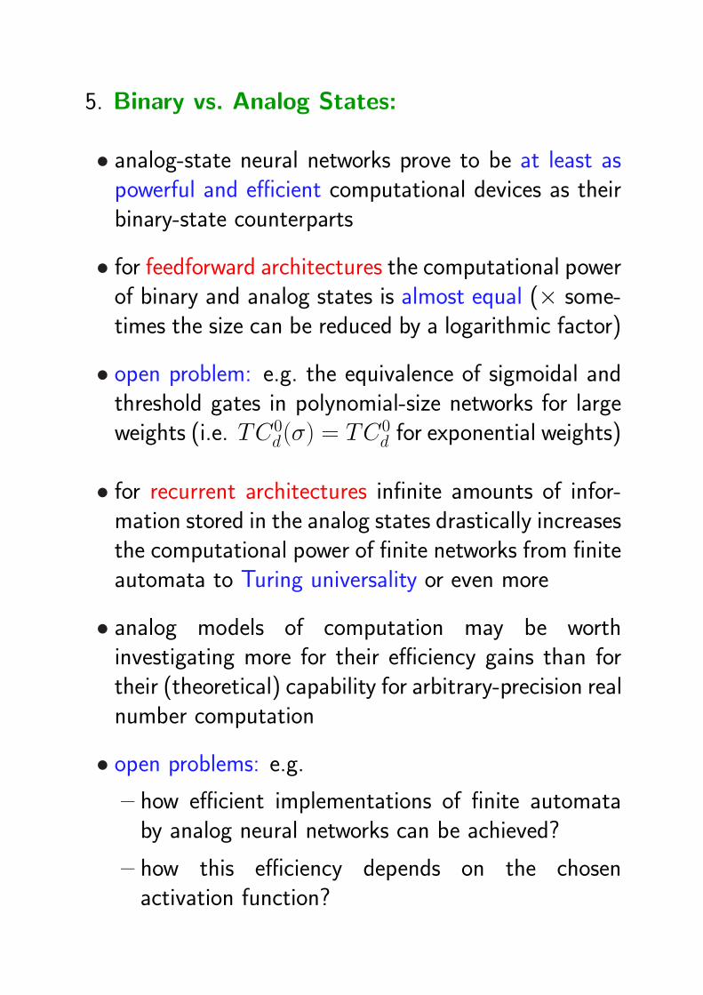
5. Binary vs. Analog States:
• analog-state neural networks prove to be at least aspowerful and efficient computational devices as theirbinary-state counterparts
• for feedforward architectures the computational powerof binary and analog states is almost equal (× some-times the size can be reduced by a logarithmic factor)
• open problem: e.g. the equivalence of sigmoidal andthreshold gates in polynomial-size networks for largeweights (i.e. TC0
d(σ) = TC0d for exponential weights)
• for recurrent architectures infinite amounts of infor-mation stored in the analog states drastically increasesthe computational power of finite networks from finiteautomata to Turing universality or even more
• analog models of computation may be worthinvestigating more for their efficiency gains than fortheir (theoretical) capability for arbitrary-precision realnumber computation
• open problems: e.g.
– how efficient implementations of finite automataby analog neural networks can be achieved?
– how this efficiency depends on the chosenactivation function?
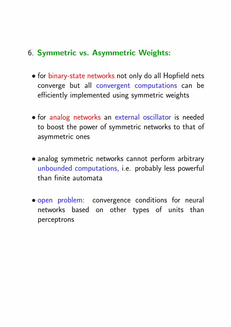
6. Symmetric vs. Asymmetric Weights:
• for binary-state networks not only do all Hopfield netsconverge but all convergent computations can beefficiently implemented using symmetric weights
• for analog networks an external oscillator is neededto boost the power of symmetric networks to that ofasymmetric ones
• analog symmetric networks cannot perform arbitraryunbounded computations, i.e. probably less powerfulthan finite automata
• open problem: convergence conditions for neuralnetworks based on other types of units thanperceptrons
Literature on Complexity Theory
of Neural Networks
• Anthony, M. (2001). Discrete Mathematics of NeuralNetworks: Selected Topics. Philadelphia, PA: Societyfor Industrial and Applied Mathematics.
• Parberry, I. (1994). Circuit Complexity and NeuralNetworks. Cambridge, MA: The MIT Press
• Roychowdhury, V. P., Siu, K.-Y., & Orlitsky, A. (Eds.)(1994). Theoretical Advances in Neural Computationand Learning. Boston: Kluwer Academic Publishers
• Siegelmann, H. T. (1999). Neural Networks and Ana-log Computation: Beyond the Turing Limit. Boston:Birkhauser.
• Sıma, J., & Orponen, P. (2003). General-purposecomputation with neural networks: A survey of com-plexity theoretic results. Neural Computation, 15 (12),2727–2778. (covers most of this tutorial)
• Siu, K.-Y., Roychowdhury, V. P., & Kailath, T. (1995a).Discrete Neural Computation: A Theoretical Founda-tion. Englewood Cliffs, NJ: Prentice Hall.