ices report 13-34 locally conservative discontinuous

ICES REPORT 13-34

December 2013

Locally Conservative Discontinuous Petrov-GalerkinFinite Elements For Fluid Problems

by

Truman Ellis, Leszek Demkowicz, And Jesse Chan

The Institute for Computational Engineering and SciencesThe University of Texas at AustinAustin, Texas 78712

Reference: Truman Ellis, Leszek Demkowicz, And Jesse Chan, Locally Conservative DiscontinuousPetrov-Galerkin Finite Elements For Fluid Problems, ICES REPORT 13-34, The Institute for ComputationalEngineering and Sciences, The University of Texas at Austin, December 2013.

Locally Conservative Discontinuous Petrov-Galerkin Finite

Elements for Fluid Problems

Truman Ellis, Leszek Demkowicz, and Jesse Chan

Institute for Computational Engineering and Sciences,The University of Texas at Austin,

Austin, TX 78712

Abstract

We develop a locally conservative formulation of the discontinuous Petrov-Galerkin finite elementmethod (DPG) for convection-diffusion type problems using Lagrange multipliers to exactly enforceconservation over each element. We provide a proof of convergence as well as extensive numerical ex-periments showing that the method is indeed locally conservative. We also show that standard DPG,while not guaranteed to be conservative, is nearly conservative for many of the benchmarks considered.The new method preserves many of the attractive features of DPG, but turns the normally symmetricpositive-definite DPG system into a saddle-point problem.

1 Introduction

The discontinuous Petrov-Galerkin (DPG) method with optimal test functions has been under active devel-opment for convection-diffusion type systems [10, 11, 15, 3, 16, 5, 19]. In this paper, we develop a theoryfor the locally conservative formulation of DPG for convection-diffusion type equations (including Burgers’Equation and Stokes flow) and supplement this with extensive numerical results.

1.1 Importance of Local Conservation

Locally conservative methods hold a special place for numerical analysts in the field of fluid dynamics.Perot[20] argues

Accuracy, stability, and consistency are the mathematical concepts that are typically used toanalyze numerical methods for partial differential equations (PDEs). These important toolsquantify how well the mathematics of a PDE is represented, but they fail to say anything abouthow well the physics of the system is represented by a particular numerical method. In practice,physical fidelity of a numerical solution can be just as important (perhaps even more important toa physicist) as these more traditional mathematical concepts. A numerical solution that violatesthe underlying physics (destroying mass or entropy, for example) is in many respects just asflawed as an unstable solution.

There are also some mathematically attractive reasons to pursue local conservation. The Lax-Wendrofftheorem guarantees that a convergent numerical solution to a system of hyperbolic conservation laws willconverge to the correct weak solution.

The discontinuous Petrov-Galerkin finite element method has been described as least squares finite ele-ments with a twist. The key difference is that least squares methods seek to minimize the residual of thesolution in the L2 norm, while DPG seeks the minimization in a dual norm realized through the inverseRiesz map. Exact mass conservation has been an issue that has long plagued least squares finite elements.Several approaches have been used to try to adress this. Bochev et al. [1] accomplish local conservation byusing a pointwise divergence free velocity space in the Stokes formulation. Chang and Nelson[6] developed

1

the restricted LSFEM [6] by augmenting the least squares equations with Lagrange multipliers explicitlyenforcing mass conservation element-wise. Our conservative formulation of DPG takes a similar approachand both methods similarly share the disadvantage of transforming a minimization method to a saddle-pointproblem. In the interest of crediting Chang and Nelson’s restricted LSFEM, we call the following locallyconservative DPG method the restricted DPG method (RDPG).

1.2 DPG is a Minimum Residual Method

Roberts et al. presents a brief history and derivation of DPG with optimal test functions in [21]. We followhis derivation of the standard DPG method as a minimum residual method. Let U be the trial Hilbert spaceand V the test Hilbert space for a well-posed variational problem b(u, v) = l(v). In operator form this isBu = l, where B : U → V ′ and 〈Bu, v〉 = b(u, v). We seek to minimize the residual for the discrete spaceUh ⊂ U :

uh = arg minuh∈Uh

1

2‖Buh − l‖2V ′ . (1)

Recalling that the Riesz operator RV : V → V ′ is an isometry defined by

〈RV v, δv〉 = (v, δv)V , ∀δv ∈ V,

we can use the Riesz inverse to minimize in the V -norm rather than its dual:

1

2‖Buh − l‖2V ′ =

1

2

∥∥R−1V (Buh − l)

∥∥2

V=

1

2

(R−1V (Buh − l), R−1

V (Buh − l))V. (2)

The first order optimality condition for (2) requires the Gateaux derivative to be zero in all directionsδu ∈ Uh, i.e., (

R−1V (Buh − l), R−1

V Bδu)V

= 0, ∀δu ∈ U.

By definition of the Riesz operator, this is equivalent to⟨Buh − l, R−1

V Bδuh⟩

= 0 ∀δuh ∈ Uh . (3)

Now, we can identify vδuh:= R−1

V Bδuh as the optimal test function for trial function δuh. Define T :=R−1V B : Uh → V as the trial-to-test operator. Now we can rewrite (3) as

b(uh, vδuh) = l(vδuh

). (4)

The DPG method then is to solve (4) with optimal test functions vδuh∈ V that solve the auxiliary problem

(vδuh, δv)V = 〈RV vδuh

, δv〉 = 〈Bδuh, δv〉 = b(δuh, δv) , ∀δv ∈ V. (5)

Using a continuous test basis would result in a global solve for every optimal test function. ThereforeDPG uses a discontinuous test basis which makes each solve element-local and much more computationallytractable. Of course, (5) still requires the inversion of the infinite-dimensional Riesz map, but approximatingV by a finite dimensional space, Vh, which is of a higher polynomial degree than Uh (hence “enriched space”)works well in practice.

No assumptions have been made so far on the definition of the inner product on V . In fact, proper choiceof (·, ·)V can make the difference between a solid DPG method and one that suffers from robustness issues.

2 Element Conservative Convection-Diffusion

We now proceed to develop a locally conservative formulation of DPG for convection-diffusion type problems,but there are a few terms that we need to define first. If Ω is our problem domain, then we can partition itinto finite elements K such that

Ω =⋃K

K, K open,

2

with corresponding skeleton Γh and interior skeleton Γ0h,

Γh :=⋃K

∂K Γ0h := Γh − Γ.

We define broken Sobolev spaces element-wise:

H1(Ωh) :=∏K H

1(K),

H(div,Ωh) :=∏KH(div,K).

We also need the trace spaces:

H12 (Γh) :=

v = vK ∈

∏K H

1/2(∂K) : ∃v ∈ H1(Ω) : v|∂K = vK,

H−12 (Γh) :=

σn = σKn ∈

∏K H

−1/2(∂K) : ∃σ ∈H(div,Ω) : σKn = (σ · n)|∂K,

which are developed more precisely in [21].

2.1 Derivation

Now that we have briefly outlined the abstract DPG method, let us apply it to the convection-diffusionequation. The strong form of the steady convection-diffusion problem with homogeneous Dirichlet boundaryconditions reads

∇ · (βu)− ε∆u = f in Ωu = 0 on Γ ,

where u is the property of interest, β is the convection vector, and f is the source term. NonhomogeneousDirichlet and Neumann boundary conditions are straightforward but would add technicality to the followingdiscussion. Let us write this as an equivalent system of first order equations:

∇ · (βu− σ) = f

1

εσ −∇u = 0 .

If we then multiply the first equation by some scalar test function v and the bottom equation by somevector-valued test function τ , we can integrate by parts over each element K:

−(βu− σ,∇v)K + ((βu− σ) · n, v)∂K = (f, v)K

1

ε(σ, τ )K + (u,∇ · τ )K − (u, τn)∂K = 0 .

(6)

The discontinuous Petrov-Galerkin method refers to the fact that we are using discontinuous optimal testfunctions that come from a space differing from the trial space. It does not specify our choice of trial space.Nevertheless, many versions of DPG in the literature (convection-diffusion [12], linear elasticity [2], linearacoustics [14], Stokes [21]) associate DPG with the so-called “ultra-weak formulation.” We will follow thesame derivation for the convection-diffusion equation, but we emphasize that other formulations are available(in particular, the Primal DPG[9] method presents an alternative with continuous trial functions). Thus,we seek field variables u ∈ L2(K) and σ ∈ L2(K). Mathematically, this leaves their traces on elementboundaries undefined, and in a manner similar to the hybridized discontinuous Galerkin method, we definenew unknowns for trace u and flux t. Applying these definitions to (6) and adding the two equations together,we arrive at our desired variational problem.

Find u := (u,σ, u, t) ∈ U := L2(Ωh)×L2(Ωh)×H1/2(Γh)×H−1/2(Γh) such that

−(βu− σ,∇v)K + (t, v)∂K +1

ε(σ, τ )K + (u,∇ · τ )K − (u, τn)∂K︸︷︷︸

b(u,v)

= (f, v)K︸︷︷︸l(v)

in Ω (7)

u = 0 on Γ (8)

3

for all v := (v, τ ) ∈ V := H1(Ωh)×H(div,Ωh).We note that, for convection-diffusion problems, we are particularly interested in designing a robust DPG

method. Specifically, we are interested in designing methods whose behavior does not change as the diffusionparameter ε becomes very small. Naive Galerkin methods for convection-diffusion tend to suffer from a lackof robustness; specifically, the finite element error is bounded by a constant factor of the best approximationerror, but the constant is often proportional to ε−1. Our aim is to design a DPG method with this inmind. We follow the methodology introduced by Heuer and Demkowicz in [16]: the ultra-weak variationalformulation for convection-diffusion can be refactored as

b((u,σ, u, t

), (τ , v)

)=∑K∈Ωh

[⟨t, v⟩δK

+ 〈u, τn〉δK + (u,∇ · τ − β · ∇v)L2(K) +

(σ,

1

ετ +∇v

)L2(K)

],

modulo application of boundary data. If we choose specific conforming test functions satisfying the adjointequations

∇ · τ − β · ∇v = u,

1

ετ +∇v = σ,

then evaluating b((u,σ, u, fn

), (τ , v)

)at these specific test functions returns back ‖u‖2 + ‖σ‖2, the L2

norm of our field variables. Multiplying and dividing through by the test norm ‖v‖V , we have

‖u‖2L2(Ω) + ‖σ‖2L2(Ω) = b((u,σ, u, fn

), (τ , v)

)=b((u,σ, u, fn

), (τ , v)

)‖v‖V

‖v‖V ≤∥∥∥u,σ, u, fn∥∥∥

E‖v‖V ,

where ∥∥∥u,σ, u, fn∥∥∥E

= supv∈V \0

b((u,σ, u, fn

), (τ , v)

)‖v‖V

is the DPG energy norm. If we can robustly bound the test norm ‖v‖V .(‖u‖2L2(Ω) + ‖σ‖2L2(Ω)

)1/2

(i.e.

derive a bound from above with a constant independent of ε), then we can divide through to get(‖u‖2L2(Ω) + ‖σ‖2L2(Ω)

) 12

.∥∥∥u,σ, u, fn∥∥∥

E. (9)

In other words, the energy norm in which DPG is optimal bounds independently of ε the L2 norm; as wedrive our energy error down to zero, we can expect that the L2 error will also decrease regardless of ε.

We note that the construction of the test norm ‖v‖V for a robust DPG method depends on two things: thetest norm, as well as the adjoint equation. In [16], the standard problem with Dirichlet conditions enforcedover the entire boundary was considered; in [5], boundary conditions were chosen for the forward problemsuch that the induced adjoint problem was regularized and contained no strong boundary layers, allowing forthe construction of a stronger test norm on V . We adopt a slight modification of the test norm introducedin [5] for numerical experiments here, which is motivated and explained in more detail in Section 2.3.1.

Having reviewed and laid the foundation for DPG methods, we can now formulate our conservative DPGscheme. Let Uh := Uh × Sh × Uh × Fh ⊂ L2(Ωh) × L2(Ωh) ×H 1

2 (Γh) ×H− 12 (Γh) be a finite-dimensional

subspace, and let uh := (uh.σh, uhth) ∈ Uh be the group variable. The element conservative DPG schemeis derived from the Lagrangian:

L(uh, λk) =1

2

∥∥R−1V (b(uh, ·)− (f, ·))

∥∥2

V−∑K

λK(b(uh, (1K ,0))− l((1K ,0))) , (10)

where (1K ,0) is the test function in which v = 1 on element K and 0 elsewhere and τ = 0 everywhere.Taking the Gateaux derivatives as before, we arrive at the following system of equations:

b(uh, T (δuh))−∑K λKb(uh, (1K ,0)) = l(T (δuh)) ∀δuh ∈ Uh

b(uh, (1K ,0)) = l((1K ,0)) ∀K ,(11)

4

where T := R−1V B : Uh → V is the same trial-to-test operator as in the original formulation.

Denote T (δuh) = (vδuh, τ δuh

) ∈ H1(Ωh)×H(div,Ωh). Then, putting (11) into more concrete terms forconvection-diffusion, we get:

−(βu− σ,∇vδuh) + 〈t, vδuh

〉+ 1ε (σ, τ δuh

) + (u,∇ · τ δuh)− 〈u, τ δuh

· n〉−∑K λK(δt, (1K ,0)) = (f, vδuh

) ∀δuh ∈ Uh

〈t, (1K ,0)〉 = (f, 1K) ∀K .(12)

2.2 Stability Analysis

In the following analysis, we neglect the error due to the approximation of optimal test functions. We followthe classical Brezzi’s theory [?, 8] for an abstract mixed problem: u ∈ U , p ∈ Q

a(u,w) + c(p,w) = l(w) ∀w ∈ Uc(q,u) = g(q) ∀q ∈ Q

(13)

where U , Q are Hilbert spaces, and a, c, l, q denote the appropriate bilinear and linear forms. Note thata(u,w) = b(u, Tw) = (Tu, Tw)V in the notation from the previous section.

Let function ψ denote the H(div,Ω) extension of flux t that realizes the minimum in the definition of thequotient (minimum energy extension) norm. The choice of norm for the Lagrange multipliers λK is impliedby the quotient norm used for H−1/2(Γh) and continuity bound for form c(p,w) representing the constraint:

|c(∑K λK(1K ,0), (u,σ, u, t))| = |

∑K λK〈t, 1K〉∂K |

= |∑K λK〈vn, 1K〉∂K |

= |∑K λK

∫K

divψ 1K |

≤∑K λK ||divψ||L2(K)µ(K)1/2

≤ (∑K µ(K)λ2

K)1/2 (∑K ||divψ||2L2(K))

1/2

≤ (∑K

µ(K)λ2K)1/2

︸︷︷︸=:||λ||

||t||H−1/2(Γh)

(14)

where µ(K) stands for the area (measure) of element K.We proceed now with the discussion of the discrete inf-sup stability constants. We skip index h in the

notation.

Inf Sup Condition relating spaces U and Q reads as follows,

supw∈U

|c(p,w)|||w||U

≥ β||p||Q (15)

LetR : L2(Ω) 3 q → ψ ∈H(div,Ω) ∩H1(Ω) = H1(Ω) (16)

be the continuous right inverse of the divergence operator constructed by Costabel and McIntosh in [7]. Letψh denote the classical, lowest order Raviart-Thomas (RT) interpolant of function

ψ = R(∑K

λK1K) . (17)

Note that divψh = divψ = λK in element K.

5

Classical h-interpolation interpolation error estimates for the lowest error Raviart-Thomas elements andcontinuity of operator R imply the stability estimate:

||ψh|| ≤ ||ψh −ψ||+ ||ψ||

≤ Ch||ψ||H1 + ||ψ||

≤ C||divψ|| = C(∑K µ(K)λ2

K)1/2

(18)

Above, C is a generic, mesh independent constant incorporating constant from the interpolation error esti-mate and continuity constant of R. Let t be now the trace of ψh. We have then,

supt∈H−1/2(Γh)

|∑K λK〈t, 1K〉∂K |||t||H−1/2(Γh)

≥|∑K λK

∫K

divψh 1K |||ψh||H(div,Ω)

≥ 1

C(∑K

µ(K)λ2K)1/2 (19)

where C is the constant from stability estimate (18).Notice that we have considered traces of lowest order Raviart-Thomas elements for the discretization of

flux t. The inf-sup condition for the lowest order RT spaces implies automatically the analogous conditionfor elements of arbitrary order; increasing the dimension of space U only makes the discrete inf-sup constantbigger.

Inf Sup in Kernel Condition is satisfied automatically due to the use of optimal test functions. Firstof all, we characterize the “kernel” space:

U0 := w ∈ U : c(q,w) = 0 ∀q ∈ Q

= (u,σ, u, t) : 〈t, 1K〉 = 0 ∀K(20)

In other words, the kernel space contains only the equilibriated fluxes. With u ∈ U0, we have then:

supw∈U0

|a(u,w)|||w||U

≥ |b(u, Tu)|||u||

=|b(u, Tu)|||Tu||

||Tu||||u||

= sup(v,τ )

|b((u,σ, u, t), (v, τ ))|||(v, τ )||

||Tu||||u||

≥ γ2||(u,σ, u, t)|| (21)

where γ is the stability constant for the standard continuous DPG formulation. The first inequality followsas we plug in the definition for a and pick w = u. The second equality is trivial, while the next one followsby definition of the optimal test functions given through the trial-to-test operator T . The finally inequality

springs from the fact that supv|b(u,v)|||v|| ≥ γ||u|| and ||Tu||V = ||R−1

V Bu||V = ||Bu||V ′ ≥ γ||u||.With both discrete inf-sup constants in place, we have the standard result: the FE error is bounded by

the best approximation error. Notice that the exact Lagrange multipliers are zero, so the best approximationerror involves only solution (u,σ, u, t).

2.2.1 Robustness Analysis

Recall the line of analysis leading to the construction of robust test norms allowing us to bound the L2 errorof the field variables by the energy error, Equation 9. With robust test norms, we have(

||u− uh||2 + ||σ − σh||2) 1

2 . ||(u− uh,σ − σh, u− uh, t− th||E

= inf(wh,ςh,w,rh) ||(u− wh,σ − ςh, u− wh, t− rh||E .(22)

The last equality follows from the fact that DPG method delivers the best approximation error in the energynorm (minimizes the residual). This is no longer true for the restricted version. So, can we claim robustnessin the sense of the inequality above for the restricted version as well?

One possible way to attack the problem is to switch to the energy norm in the Brezzi’s stability analysis.Dealing with the “inf-sup in kernel” condition is simple. Upon replacing the original norm of solution uwith the energy norm, both constant γ and continuity constant become unity. In order to investigate the

6

robustness of inf-sup constant β, we need to realize first what the energy norm of flux t is. Given an elementK, we solve for the optimal test functions corresponding to flux t,

vK ∈ H1(K), τK ∈H(div,K)

((vK , τK), (δv, δτ ))V = 〈t, δv〉∂K ∀δv ∈ H1(K), δτ ∈H(div,K) .(23)

The energy norm of t is then equal to

||t||2E =∑K

||(vK , τK)||2V . (24)

We need to establish sufficient conditions under which the inf-sup and continuity constants for the bilinearform representing the constraint are independent of viscosity ε.

Let us start with the inf-sup condition,

supt

|∑K λK〈t, 1K〉|||t||E

≥ β

(∑K

µ(K)λ2K

)1/2

. (25)

As in the previous analysis, we select for t the trace of Raviart-Thomas interpolant ψh of ψ = R(∑K λK1K)

where R is the right-inverse of the divergence operator constructed by Costabel and McIntosh. The onlychange compared with the previous analysis, is the evaluation of norm of th. For this, we need to solve thelocal problems:

((v, τ ), (δv, δτ )V = 〈t, δv〉∂K =

∫K

divψh δv =

∫K

divψ δv

=

∫K

λKδv = λK(1K , δv)K ∀δv ∈ H1(K)∀δτ ∈H(div,K) (26)

We need then an upper bound of the energy norm of (vh, τh):(∑K

||(v, τ )||2V

)1/2

.

Substituting (v, τ ) for (δv, δτ ) in (26), we get,

||(v, τ )||2V = λK(1K , vK) (27)

If we have a robust stability estimate:

(1K , vK) ≤ Cµ(K)1/2||(v, τ )||K (28)

(i.e. constant C is independent of ε) then

||(v, τ )||V ≤ Cµ(K)1/2|λK | (29)

and, eventually, as needed, ∑K

||(v, τ )||2V ≤ C2∑K

µ(K)λ2K (30)

which leads to the robust estimate of inf-sup constant β. For example, it is sufficient if

||v||L2(K) ≤ ||(v, τ )||V . (31)

Notice that the stability analysis with the energy norm was, in a sense, easier than with the quotient norm.Only the divergence of the interpolant ψh enters (26) and it coincides with the divergence of ψ.

7

We arrive at a similar situation in the continuity estimate of∑K

λK〈t, 1K〉 .

Testing with (1K ,0) in the local problem (23), we obtain,

((v, τ ), (1K ,0))V = 〈t, 1K〉∂K (32)

If we have a robust estimate,

|((v, τ ), (1K ,0))V | ≤ Cµ(K)1/2 ||(v, τ )||V (33)

then|∑K

λK〈t, 1K〉| ≤ C(∑K

µ(K)λ2K)1/2 (

∑K

||(v, τ )||2V )1/2 = C(∑K

µ(K)λ2K)1/2||t||E (34)

as needed.For instance, condition (33) will be satisfied if the test inner product in (32) reduces to the L2 term only,

((v, τ ), (1K ,0))V = (v, 1K)L2(K) . (35)

With the robust stability and continuity constants for the mixed problem, the energy error of solution(u,σ, u, t) (and Lagrange multipliers λK as well) is bounded robustly by the best approximation error of(u,σ, u, t) measured in the energy norm. We arrive thus at the same situation as in the standard DPGmethod.

2.3 Robust test norms

The optimal test functions are determined by solving local problems determined by the choice of test norm.There are several options to consider. The graph norm [13] is one of the most natural norms to consider asit is derived directly from the adjoint of the problem supplemented with (possibly scaled) L2 field terms toupgrade it from a semi-norm. Chan et al. [5] derived a more robust alternative norm for convection diffusion(dubbed the robust norm). We recently developed a modification of the robust norm that appears to producebetter results in the presence of singularities. In this section we illustrate the singularity issues with theLaplace equation, offer possible explanations for the phenomena observed, and propose a modification of therobust test norm, which we demonstrate eliminates the issues observed in numerical experiments.

2.3.1 A model problem

We begin by first examining a different problem than convection-diffusion. We look at admissible solutionsfor the homogeneous Laplace’s equation (convection diffusion with β = 0) over the y > 0 half-plane underboundary conditions

u = 0 on x > 0

∂u

∂n= 0 on x < 0.

Let us consider the 2D case - a simple separation of variables argument in polar coordinates shows that thesolution is of the form

u(r, θ) =

∞∑n=0

Rn(r) sin(λnθ),

where λn = n + 12 , and Rn(r) = C1,nx

λn + C2,nx−λn . By requiring u(0, θ) < ∞, we have Rn(r) = Cnx

λn .We have now that solutions to this problem include u of the form

u =∑n=0

xn+ 12 sin

((n+

1

2

)θ

).

8

Note that in the lowest-order term, the gradient of u displays a singularity at r = 0. It is well known that,for smooth boundary data, solutions to Laplace’s equation can be decomposed into the linear combinationof smooth and singular contributions; the above analysis implies that, when boundary conditions changefrom Dirichlet to Neumann on the half-plane, the Laplace’s equation will always develop a singularity in thestresses.

Consider now Laplace’s equation ∆u = f on the box domain Ω = [0, 1]2 with boundary conditions

u = 0 on x > .5

∂u

∂n= 0 on x < .5.

with forcing term f = 1. Extrapolating the results from the half-plane example to a finite domain, we

Figure 1: Solution of Laplace’s equation on the unit quad with f = 1.

expect the solution of Laplace’s equation to be bounded, but to have a singularity in its gradient. Figures 1and 2 are finite element solutions of the above problem obtained with a quadratic h-refined mesh. Figure 1confirms that u is bounded, while Figure 2 confirms that singularities in the gradient appear at the point(.5, 0), where the boundary condition changes from Neumann to Dirichlet.

We consider now the convection-diffusion problem, under a similar setup as before. We consider thedomain Ω = [0, 1]2 with advection vector β = (1, 0) and boundary conditions

u = 0, on x = 0

∂u

∂n= 0, on x = 1, y = 1, and y = 0, x < .5

u = 1, on .5 < x ≤ 1.

The problem is meant to simulate the transport of u over a domain with a “plate” boundary x ∈ [.5, 1].For small ε, the problem develops a boundary layer over the plate, as well as a singularity at the plate tip(x, y) = (.5, 0).1 Unlike the Laplace example, we swap the Dirichlet boundary condition at the outflow x = 1with an outflow boundary condition.2

1This problem is meant to mimic the Carter flat plate problem – a common early benchmark problem in viscous compressibleflow problems – which can be shown to also exhibit a singularity in stress at the point (.5, 0).

2The outflow “boundary condition” is simply the absence of an applied boundary condition, and is analyzed in more detail in

9

Figure 2: x and y components of the ∇u for u solving Laplace’s equation with a change in boundaryconditions. Both components develop singularities at the point where the boundary condition changes type.

The above convection-diffusion problem is related back to the earlier Laplace/diffusion problem with asingularity – in most of the domain, convective effects dominate; however, localizing the behavior of Laplace’sequation to a circle of ε around (.5, 0), we again see a discontinuity in the stresses. Asymptotic expansiontechniques indicate that singularities in solutions are determined primarily by the highest order differentialoperator present in the equation – in other words, the addition of a convective term to a scaled Laplacian(to recover the convection-diffusion equation) will not alter the presence of a singularity in the solution [22].

Figure 3: Solution u for ε = .01 under the robust test norm. The solution oscillates strongly at the plateedge, growing in magnitude under additional refinements despite the absence of a singularity in u at thatpoint.

Figures 3 and 4 demonstrate the behavior of the DPG method under the robust test norm for the plateproblem. The diffusion is taken to be fairly large (ε = 10−2), and automatic refinements are done until theelement size h is at or below the diffusion scale. Due to the singular nature of the solution, refinements areclustered around (.5, 0), and the order is set to be uniform with p = 2. While there should be no singularityin u, the magnitude of u grows as h→ 0, so long as h ≤ ε.

[18]. This outflow condition appears to work well for convection-diffusion problems in the convective regime, and is the outflowcondition we will use in our extension of DPG to a model problem in viscous compressible flow. Though the well-posedness ofthe problem under this boundary condition is questionable, we can still effectively illustrate the issues present under the robusttest norm using this problem setup.

10

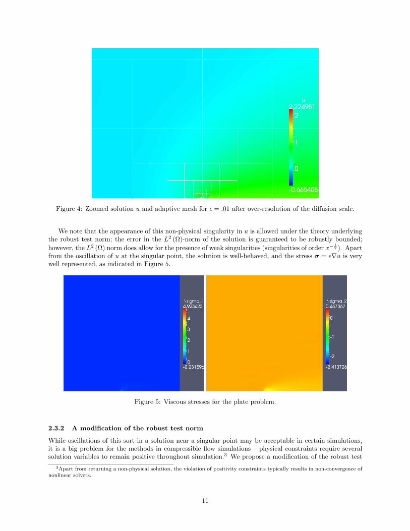
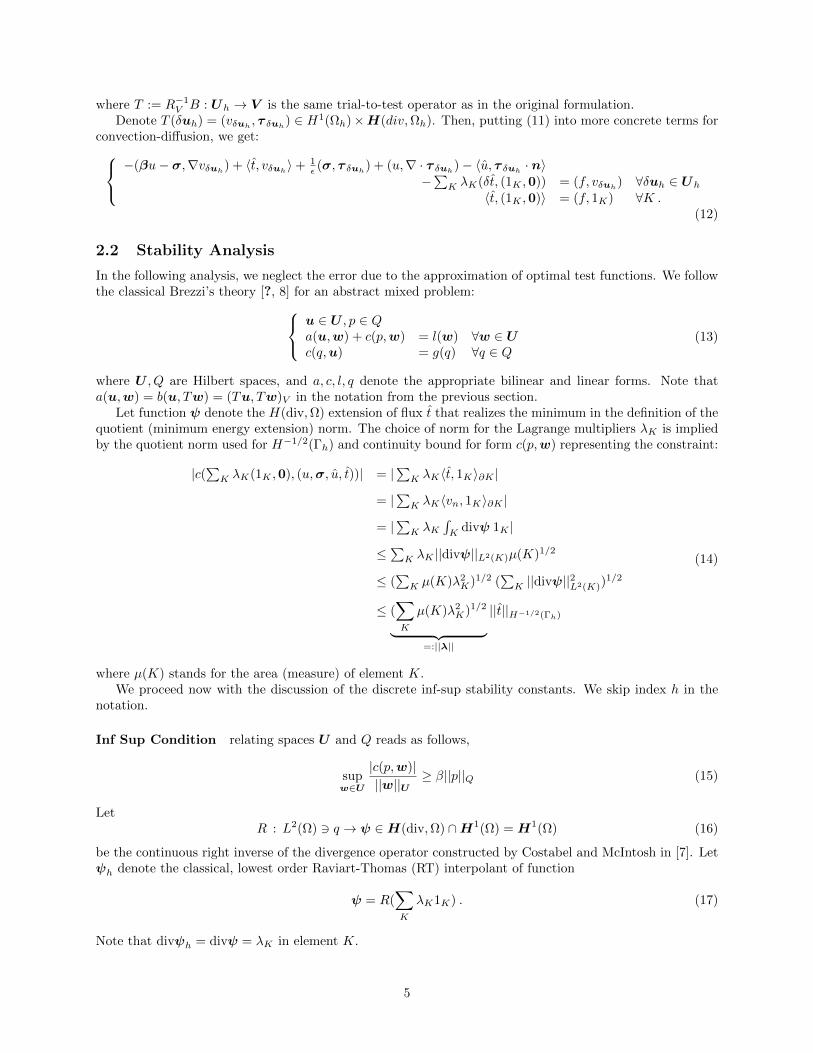
Figure 4: Zoomed solution u and adaptive mesh for ε = .01 after over-resolution of the diffusion scale.

We note that the appearance of this non-physical singularity in u is allowed under the theory underlyingthe robust test norm; the error in the L2 (Ω)-norm of the solution is guaranteed to be robustly bounded;

however, the L2 (Ω) norm does allow for the presence of weak singularities (singularities of order x−12 ). Apart

from the oscillation of u at the singular point, the solution is well-behaved, and the stress σ = ε∇u is verywell represented, as indicated in Figure 5.

Figure 5: Viscous stresses for the plate problem.

2.3.2 A modification of the robust test norm

While oscillations of this sort in a solution near a singular point may be acceptable in certain simulations,it is a big problem for the methods in compressible flow simulations – physical constraints require severalsolution variables to remain positive throughout simulation.3 We propose a modification of the robust test

3Apart from returning a non-physical solution, the violation of positivity constraints typically results in non-convergence ofnonlinear solvers.

11

norm that appears to remedy this issue, which we refer to as the coupled robust test norm:

‖(v, τ )‖2V,K := min

1

ε,

1

µ(K)

‖τ‖2K ,+ ‖∇ · τ − β · ∇v‖

2K (36)

+ ‖β · ∇v‖2K + ε ‖∇v‖2K + ‖v‖2K (37)

where || · ||K signifies the L2 norm over element K.4 We note that, under the theory developed in [5] theabove test norm is trivially provably robust using the same ideas.5

While not rigorously understood, we believe the issues related to the appearance of non-physical singular-ities to be related to the uncoupled nature of the test norm. Previous example problems exhibited boundarylayers and sharp gradients in the stress σ, but not singularities, which contribute significantly more error.We expect that the oscillations observed in u are a sort of pollution error, where error in u is tied to errorin σ. If we consider the ultra-weak variational formulation for convection-diffusion

(u,∇ · τ − β · ∇v)L2(Ω) +

(σ,

1

ετ +∇v

)L2(Ω)

+ . . . ,

we can see that it is a combination of test functions that corresponds to both u and σ. Referring to [5], wenote that, by choosing τ and v such that they satisfy the adjoint equation with forcing terms u and σ, werecover the best L2 approximation. In other words, achieving optimality in the L2 norm requires couplingbetween v and τ , which is achieved under the graph norm, but not the robust norm derived in the previoussection. If coupling of the test terms delivers optimality in u and σ independently, we expect that decouplingv and τ from each other in a test norm will have the effect of coupling error in σ to error in u, which wouldexplain the spurious oscillations in u in the presence of singularities in σ. Similar results have been observedin the Stokes equations, where error in u is coupled to the behavior of the pressure variable [17].

The drawback to using the above test norm is that the resulting local system for test functions is nowcompletely coupled, whereas using the robust test norm, the system was block diagonal due to the decouplingin v and τ and could be constructed and inverted more efficiently. We hope to explore the difference betweenthese two norms in more rigor and detail in the future.

Figure 6: ε = 10−2 without h-resolving diffusion scale, and with h-resolution of diffusion scale.

Figure 6 shows the solution for ε = .01, where the diffusion scale is both under-resolved and resolved byh-adaptivity. In both cases, there are no oscillations near the plate tip – Figure 7 shows a zoomed image of

4We note that we have dropped the mesh-dependent scaling on ‖v‖L2(Ω) from the robust norm; this is related to recent

insights into the nature of DPG test spaces as discussed in [4].5This is due to the fact that ‖∇ · τ − β · ∇v‖2L2(Ω) is robustly bounded by ‖∇ · τ‖L2(Ω) and ‖β · ∇v‖L2(Ω). Alternatively,

we can note that ‖∇ · τ − β · ∇v‖2L2(Ω) = ‖g‖2L2(Ω), where g is a load of the adjoint problem related to robustness described

in [5].

12

the solution u at the point (.5, 0). The stress is resolved similarly to the previous case; however, the solutionu does not display spurious oscillations in either the under-resolved or resolved cases. Figure 8 displaysthe same quantities, but for ε = 10−4, in order to demonstrate that the new test norm removes spuriousoscillations in u (in the presence of singularities in σ) independently of ε.

Figure 7: Zoom of solution u at the plate tip for ε = 10−2.

Figure 8: 14 refinements for ε = 10−4, min h is O(10−5).

2.3.3 Adaptation for a Locally Conservative Formulation

With this choice of test norm, our local problem now becomes:Find vδuh

∈ H1(K), τ δuh∈H(div,K) such that:

min

1

ε,

1

µ(K)

(τ δuh

, δτ )K + (∇ · τ δuh− β · ∇v,∇ · δτ − β · ∇v)K + (β · ∇vδuh

,β · ∇δv)K

+ ε(∇vδuh,∇δv)K + α(vδuh

, δv)K = b(δuh, (δv, δτ )) ∀δv ∈ H1(K), δτ ∈H(div,K) , (38)

where, typically, α = 1.With a locally conservative formulation, we can pass in local problem (38) with α → 0. The fact that

the test functions will be determined then up to a constant does not matter, for δt ∈ F eh , equation (12)1 isorthogonal to constants. Mathematically, we are dealing with equivalence classes of functions, but in order

13

to obtain a single function that we can deal with numerically, we replace the alpha term with a zero meanscaling condition to obtain the new test norm,

min

1

ε,

1

µ(K)

(τ δuh

, δτ )K + (∇ · τ δuh− β · ∇v,∇ · δτ − β · ∇v)K (39)

+ (β · ∇vδuh,β · ∇δv)K + ε(∇vδuh

,∇δv)K +1

µ(K)

∫K

vδuh

∫K

δv

where the 1µ(K) coefficient is an arbitrary scaling condition that doesn’t make a difference mathematically,

but can affect the condition number of the actual solve. In practice, we use 1µ(K)2 since

∫Kvδuh

and∫Kδv

both scale like µ(K), but 1µ(K) is more convenient more the analysis in the next section. It is convenient to

be able to take α→ 0 as we will see in some later numerical experiments.

2.3.4 Proof of Robust Stability Estimate

In the robustness analysis in Section 2.2.1, we argued that if we have a robust stability estimate:

(1K , vK) ≤ Cµ(K)1/2||(v, τ )||K (28)

and|((v, τ ), (1K ,0))V | ≤ Cµ(K)1/2 ||(v, τ )||V . (33)

We now proceed to show that the robust norms we are using satisfy this requirement. Consider the innerproduct from Equation (38), with α = 1. We wish to verify condition (28) with the norm derived from thisinner product on the right hand side. By Cauchy-Schwarz∫

K

v · 1 ≤ µ(K)1/2 ‖v‖L2(K) ≤ µ(K)1/2 ‖(v, τ )‖K (40)

where ‖(v, τ )‖K is the norm derived from the inner product. Condition 33 comes out the same since

|((v, τ ), (1K ,0))| =∑K

|(1K , vK)| ≤∑K

µ(K)1/2 ‖v, τ‖K

element-wise.Now we wish the perform the same analysis for the modified inner product in Equation (39). In this

case, condition (28) follows even more naturally as∫K

v · 1 ≤ µ(K)1/2 1

µ(K)1/2

∣∣∣∣∫K

v

∣∣∣∣ ≤ ‖(v, τ )‖K (41)

where ‖(v, τ )‖ now refers to the norm generated by inner product (39). Condition (33) follows by the samereasoning.

3 Application to Other Fluid Model Problems

Extension of these ideas to other fluid flow problems is relatively trivial. For the following problems, we justuse the graph norm for the local problems.

3.1 Inviscid Burgers’ Equation

We include the inviscid Burgers’ equation in our suite of tests because, being a nonlinear hyperbolic conser-vation law, it falls under the scope of the Lax-Wendroff theorem. The inviscid Burger’s equation is

∂u

∂t+ u

∂u

∂x= f .

14

Define the space-time gradient: ∇xt =(∂∂x ,

∂∂t

)T. We can now rewrite this as

∇xt ·(u2/2u

)= 0 .

Multiplying by a test function v, and integrating by parts:

−((

u2/2u

),∇xtv

)+⟨t, v⟩

= (f, v) ,

where t is the trace of

(u2/2u

)· nxt on element boundaries, and nxt is the space-time normal vector. As

in convection-diffusion, local conservation implies that∫∂K

t =∫Kf for all elements, K.

In order to solve this nonlinear problem, we linearize and do a simple Newton iteration until the solutionconverges. The linearized equation is

−((

u1

)∆u,∇xtv

)+⟨t, v⟩

= (f, v) +

((u2/2u

),∇xtv

),

where u is the previous solution iteration and ∆u is the update. The results follow in Section 4.1.9.

3.2 Stokes Flow

We start with the VGP (velocity, gradient pressure) Stokes formulation:

µ∆u+∇p = f

∇ · u = 0 ,

where u is the velocity vector field. As a first order system of equations, this is

1

µσ −∇u = 0

∇ · σ +∇p = f

∇ · u = 0 ,

where σ is a tensor valued stress field. Multiplying by test functions τ (tensor valued), v (vector valued),and q (scalar valued), and integrating by parts:(

1

µσ, τ

)+ (u,∇ · τ )− 〈u, τ · n〉 = 0

− (σ,∇v)− (p,∇ · v) +⟨t,v⟩

= (f ,v)

− (u,∇q) + 〈u · n, q〉 = 0 ,

where u is the trace of u, and t is the trace of (σ + pI) · n. The solve for p is only unique up to a constant,so we also impose a zero mean condition,

∫Ωp = 0. Local conservation for Stokes flow means that over each

element,∫Ku · n = 0. Results follow in Sections 4.1.10 and 4.1.11.

4 Numerical Experiments

In 4.1 we define each numerical experiment, and in 4.2 we discuss the solution properties in general. Wesolve with second order field variables and flux (u, σ, and t), third order traces (u), and fifth order testfunctions (v and τ ).

We measure flux imbalance by looping over each element in the mesh and integrating the flux over eachside and summing them together. We then integrate the source term over the volume of the element. Thetwo should match each other, and the remainder is the flux imbalance. We get the net global flux imbalanceby summing these quantities and taking the absolute value. The max local flux imbalance is the maximumabsolute value of these flux imbalances.

15

4.1 Description of Problems

Unless otherwise noted, the problem domain is Ω = [0, 1]2 and f = 0. Also note that unless otherwise noted,for all of the pseudo-color plots, blue corresponds to 0 and red to 1 with a linear scaling in between. Also,all convection-diffusion plots are of the field variable u. Inviscid Burgers’ and Stokes results will be dealtwith individually.

4.1.1 Erickson-Johnson Model Problem

The Erickson-Johnson problem is one of the few convection-diffusion problems with a known analyticalsolution. Take β = (1, 0)T and boundary conditions t = β · nu0 when βn ≤ 0, where u0 is the trace of

the exact solution, and u = 0 when βn > 0. For n = 1, 2, · · · , let λn = n2π2ε, rn = 1+√

1+4ελn

2ε , and

sn = 1−√

1+4ελn

2ε . The exact solution is

u(x, y) = C0 +

∞∑n=1

Cnexp(sn(x− 1))− exp(rn(x− 1))

rn exp(−sn)− sn exp(−sn)cos(nπy) . (42)

The exact solution for ε = 10−2, C1 = 1, and Cn 6=1 = 0 is shown in Figure 9.

4.1.2 Skewed Convection-Diffusion Problem

This is a standard convection-diffusion problem with a skewed convection vector relative to the mesh. Wetake β = (2, 1), and on the left and bottom inflow boundaries we impose t = 1− x− y while the right andtop boundaries have u = 0. We solve for ε = 10−4.

4.1.3 Double Glazing Problem

This nominal problem definition takes the same unit square domain with

β =

(2(2y − 1)(1− (2x− 1)2)

−2(2x− 1)(1− (2y − 1)2)

); u =

1 on Γright

0 else,

except that this definition for the boundary is not legal for u ∈ H 12 (Γh) which is continuous. Therefore we

use a ramp of width√ε on the right edge to go from 0 to 1. The results are for ε = 10−2.

4.1.4 Vortex Problem

This problem models a mildly diffusive vortex convecting fluid in a circle. We deal with domain Ω = [−1, 1]2,with ε = 10−4, and β = (−y, x)T . Note that β = 0 at the domain center. We have an inflow boundary

condition when β · n < 0, in which case we set t = β · n · u0 where u0 =

√x2+y2−1√

2−1which will vary from 0

at the center of boundary edges to 1 at corners. We don’t enforce an outflow boundary.

4.1.5 Wedge Problem

We devised this problem to examine the issues we were having with the singularity in the solution underthe robust test norm. The domain is a rectangle [−0.5, 0.5] × [−1, 0.5] where the triangle connecting thebottom edges with the origin at (0, 0) is removed. The convection vector β = (1, 0)T , ε = 10−1, and weapply boundary conditions t = 0 on the left inflow edge, u = 0 on the top edge, β · n · u − t = σn = 0 onthe right outflow edge, u = 1 on the leading edge of the wedge, and t = β · n · 1 on the trailing edge of thewedge.

4.1.6 Inner Layer Problem

In this problem, β = (√

32 ,

12 )T and we have a discontinuous flux inflow condition where t = 0 if y ≤ 0.2 and

t = β · n if y > 0.2. On the outflow, u = 0. We use a very small diffusion scale of ε = 10−6 which creates avery thin inner layer.

16

Figure 9: Erickson-Johnson exact solution

102 103 104 105

Degrees of Freedom

10-5

10-4

10-3

10-2

10-1

100

Err

or

L2 - NonconservativeL2 - ConservativeEnergy - NonconservativeEnergy - Conservative

Figure 10: Error in Erickson-Johnson solutions

17

102 103 104 105

Degrees of Freedom

10-17

10-15

10-13

10-11

10-9

10-7

10-5

10-3

10-1

Flux Im

bala

nce Max Local - Nonconservative

Net Global - NonconservativeMax Local - ConservativeNet Global - Conservative

Figure 11: Flux imbalance in Erickson-Johnson solutions

4.1.7 Discontinuous Source Problem

Here, β = (0.5, 1)T /√

1.25, and we have a discontinuous source term such that f = 1 when y ≥ 2x andf = −1 when y < 2x. We apply boundary conditions of t = 0 on the inflow and u = 0 on the outflow.Contrary to the other problems discussed, the solution for this problem does not range from 0 to one. Rather,the colorbar in Figure 22 is scaled to [−1.110, 0.889].

4.1.8 Hemker Problem

The Hemker problem is defined on a domain Ω = [−3, 9] × [−3, 3] \ (x, y) : x2 + y2 < 1, essentially asimplified model of flow past an infinite cylinder. We start with the initial mesh shown in Figure 24 in whichwe approximate the circle by 8 fifth order curvilinear polynomial segments. As we refine, the new elementsare fitted to better approximate an exact circle.The boundary conditions are t = β · n · 1 on the left inflowboundary, β · n · u − t = σn = 0 on the right outflow boundary, t = 0 on the top and bottom edges, andu = 1 on the cylinder. We run with ε = 10−3.

4.1.9 Inviscid Burgers’ Equation

This is a standard test problem for Burgers’ equation. The domain is a unit square. We assign boundaryconditions t = −(1 − 2x) on the bottom, t = −1/2 on the left, while t = 1/2 on the right. Since this is ahyperbolic equation, there is no need to set a boundary condition on the top.

4.1.10 Stokes Flow Around a Cylinder

This is a common problem used to stress-test local conservation properties of least squares finite elementmethods. Since DPG can be viewed as a generalized least squares methods[13], we might expect it to struggle

18

(a) Nonconservative (b) Conservative

Figure 12: Skewed convection-diffusion problem after 8 refinements

19

102 103 104 105 106

Degrees of Freedom

10-15

10-14

10-13

10-12

10-11

10-10

10-9

10-8

10-7

10-6

10-5

10-4

10-3

10-2

Flux Im

bala



Figure 13: Flux imbalance in skewed convection-diffusion solutions

with this problem as well. The problem domain is detailed in Figure 29 with inlet and outlet velocity profiles

uin = uout =

((1− y)(1 + y)

0

),

and zero flow on the cylinder and at the top and bottom walls. We use µ = with both Stokes problems andset velocity boundary conditions on u.

Bochev et al. [1] run this test with both r = 0.6 and r = 0.9; we repeat the same experiments withstandard and restricted DPG methods starting from the very coarse meshes shown in Figure 30 whileadaptively refining toward a resolved solution. The extreme pressure gradient in the r = 0.9 case obviouslymakes local conservation more challenging.

We measure mass loss much more directly in these two Stokes problems. Because fluid enters and leavesthe domain only through the inlet and outlet boundaries, we should be able to integrate the mass flux overany cross-section of the mesh and get the same value. Unfortunately, it is not mathematically well-definedto take line integrals of our field variables which only live in L2. We can, however, integrate the trace andflux variables over element boundaries. This carries the unfortunate limitation that we can only measuremass loss where there is a clear vertical mesh line. We therefore pick integration lines from the initial coarsemesh and measure the mass flux after each adaptive refinement step. The percent mass loss is thus

%mloss =

∫Γinu · nind`−

∫Su · nSd`∫

Γinu · nind`

× 100,

where S is some vertical mesh line.

4.1.11 Stokes Flow Over a Backward Facing Step

Similarly, least squares methods have historically performed very poorly when calculating Stokes flow overa backward facing step shown in Figure 34. The stress singularity at the reentrant corner seems to destroy

20


Figure 14: Double glazing problem after 5 refinements

101 102 103 104 105

Degrees of Freedom

10-18

10-16

10-14

10-12

10-10

10-8

10-6

10-4

10-2

Flux Im

bala



Figure 15: Flux imbalance in double glazing problem

21


Figure 16: Vortex problem after 6 refinements

102 103 104 105 106

Degrees of Freedom

10-16

10-15

10-14

10-13

10-12

10-11

10-10

10-9

10-8

10-7

10-6

10-5

10-4

10-3

10-2

Flux Im

bala



Figure 17: Flux imbalance in vortex solutions

22


Figure 18: Wedge problem after 16 refinements

23

102 103 104 105

Degrees of Freedom

10-17

10-15

10-13

10-11

10-9

10-7

10-5

10-3

10-1

Flux Im

bala



Figure 19: Flux imbalance in wedge solutions

local conservation. We assign parabolic inlet and outlet velocity boundary conditions

uin =

(8(y − 0.5)(1− y)

0

)and uout =

(y(1− y)

0

)and zero velocity on all other boundaries. In this problem, we solve with fourth order field and flux variables,fifth order traces, and sixth order test functions.

4.2 Analysis of Results

4.2.1 Convection-Diffusion Results

The general trend we observe from the results is that the solution quality of the standard and restrictedformulations is nearly identical once sufficiently resolved.

Another measure of solution quality is to look at the magnitude of overshoots and undershoots in thesolution. In most of the convection-diffusion problems considered (barring the discontinuous source problem)the exact solution would range exactly between 0 and 1. In the resolved solutions, the divergence from thesevalues would be negligible, but for the inner layer, in which ε = 10−6, we get overshoots and undershootsalong the separation line. For the standard formulation, the solution range for u was [−0.392, 1.342], whilethe restricted solution range was [−0.389, 1.378]. This difference is easily accounted for by the differences inrefinement patterns between the two methods.

It is clear when comparing the refinement patterns that the two methods appear to calculate slightlydifferent error representation functions (which determine which elements to adaptively refine). StandardDPG minimizes the error in the energy norm, but the Lagrange multipliers in the restricted formulationshift the solution slightly, so we should see somewhat higher error and different elements will get chosen forrefinement. The choice of test norm also plays into this calculation of the error representation function. Asdiscussed earlier, the restricted formulation allows us to throw away the L2 term on v. The inclusion of thisterm required certain assumptions on β [5] that break down for the vortex problem, where |β| → 0 in the

24


Figure 20: Inner layer problem after 8 refinements

25

102 103 104 105 106

Degrees of Freedom

10-16

10-14

10-12

10-10

10-8

10-6

10-4

10-2

Flux Im

bala



Figure 21: Flux imbalance in inner layer solutions

center of the domain. Here, we see the standard method needlessly refines in the center of the domain wherethe solution is constant. The restricted scheme is more discerning about refinements and focuses them wheresolution features are changing. In general, though, both methods appear to follow very similar refinementpatterns.

It should not come as a surprise that the standard and restricted solutions match each other so closely.The restricted formulation enforces local conservation more strictly, but if we examine the flux imbalanceplots, the standard DPG formulation is nearly conservative on its own – and appears to become moreconservative with refinement. The flux imbalance of the restricted methods appears to bounce around closeto the machine epsilon (plus a few orders of magnitude). The level of enforcement appears to creep up withmore degrees of freedom, indicating possible accruement of numerical error.

4.2.2 Burgers’ Results

Standard and restricted DPG perform nearly identically for the inviscid Burgers’ problem. It is obvious thatthe Lax-Wendroff condition of local conservation is a sufficient, but not necessary condition for numericalsolutions to hyperbolic conservation laws. We see the same behavior with the flux imbalance plots that wasso common with convection-diffusion.

4.2.3 Stokes Results

The two Stokes problems are the first ones we encounter that stress the local conservation property ofstandard DPG. With a cylinder radius of 0.6, standard DPG loses nearly 30% of the mass post-cylinder,but quickly recovers most of that with further refinement. As we increase the cylinder radius to 0.9, theproblem only exacerbates. Nearly 100% of the mass is lost in the constricted region on coarse meshes. Ittakes a much higher level of resolution to recover the mass loss. The stress singularity at the reentrant cornerof the backward facing step causes issues for standard DPG on coarse meshes. It seems that the error inapproximating the singularity outweighs the error of missed mass conservation. If we focus refinements at

26


Figure 22: Discontinuous source problem after 8 refinements

102 103 104 105 106

Degrees of Freedom

10-16

10-14

10-12

10-10

10-8

10-6

10-4

10-2

Flux Im

bala



Figure 23: Flux imbalance in discontinuous source solutions

27

Figure 24: Initial mesh for the Hemker problem

102 103 104 105 106

Degrees of Freedom

10-17

10-15

10-13

10-11

10-9

10-7

10-5

10-3

10-1

Flux Im

bala



Figure 25: Flux imbalance in Hemker problem

28

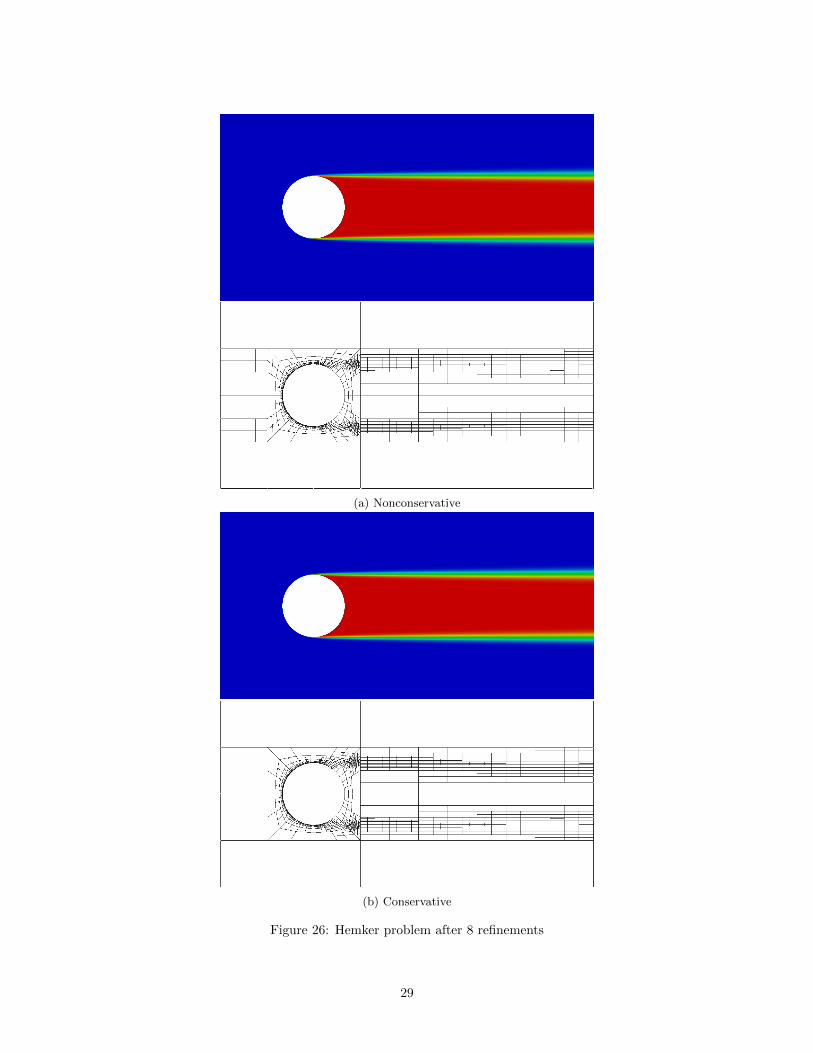
(a) Nonconservative

(b) Conservative

Figure 26: Hemker problem after 8 refinements

29


Figure 27: Burgers’ problem after 8 refinements

102 103 104

Degrees of Freedom

10-16

10-15

10-14

10-13

10-12

10-11

10-10

10-9

10-8

10-7

10-6

10-5

10-4

10-3

Flux Im

bala



Figure 28: Flux imbalance in Burgers’ solutions

30

r

-1.0

1.0

uin ucyl

3.0

uout

uwall

uwall

Figure 29: Stokes cylinder domain

(a) Mesh for r = 0.6

(b) Mesh for r = 0.9

Figure 30: Initial mesh for Stokes flow over a cylinder

31

(a) Nonconservative on initial mesh with r = 0.6 (b) Conservative on initial mesh with r = 0.6

(c) Nonconservative after 6 refinements with r = 0.6 (d) Conservative after 6 refinements with r = 0.6

(e) Nonconservative after 1 refinement with r = 0.9 (f) Conservative after 1 refinement with r = 0.9

(g) Nonconservative after 6 refinements with r = 0.9 (h) Conservative after 6 refinements with r = 0.9

Figure 31: Stokes flow around a cylinder - velocity magnitude

32

1.0 0.5 0.0 0.5 1.0 1.5 2.0 2.5 3.0x location

0

5

10

15

20

25

30

perc

ent

mass

loss

1844 DOFs7088 DOFs18728 DOFs27968 DOFs96272 DOFs171398 DOFs425276 DOFs

(a) Nonconservative

1.0 0.5 0.0 0.5 1.0 1.5 2.0 2.5 3.0x location

0.2

0.0

0.2

0.4

0.6

0.8

1.0

1.2

perc

ent

mass

loss

1e 9


(b) Conservative

Figure 32: Mass loss in Stokes flow around a cylinder of radius 0.6

33

1.0 0.5 0.0 0.5 1.0 1.5 2.0 2.5 3.0x location

0

20

40

60

80

100

perc

ent

mass

loss


(a) Nonconservative

1.0 0.5 0.0 0.5 1.0 1.5 2.0 2.5 3.0x location

2.0

1.5

1.0

0.5

0.0

0.5

1.0

1.5

2.0

2.5

perc

ent

mass

loss

1e 8


(b) Conservative

Figure 33: Mass loss in Stokes flow around a cylinder of radius 0.9

34

the singularity, the error eventually drops far enough for the method to become nearly conservative. Thesmall amount of mass loss for the restricted method is clearly due to accumulation of floating point error.

The most significant benefit of enforcing local conservation for these problems is that it allows us torecover the essential flow features with much coarser meshes. On the r = 0.6 cylinder problem, the peakvelocity magnitude of the conservative solution is fairly close on the coarsest mesh, while the nonconservativesolution severely underpredicts the peak. With the r = 0.9 cylinder, this problem is only exacerbated. Afterjust one adaptive refinement, the conservative solution nails the peak velocity. The nonconservative solutionis completely useless at this point. We see the same thing with the backward facing step problem. Theconservative solution preserves qualitative features even on the coarsest mesh, while standard DPG requiresfar higher resolution to achieve a similar solution.

5 Conclusions

We have developed a locally conservative formulation of DPG by leveraging Lagrange multipliers. While theformulation is provably convergent and robust, it does increase the number of unknowns in the system andchanges the structure from symmetric positive-definite to a saddle-point problem. Numerical results indicatethat the method delivers what it promises with local flux imbalances hovering close to machine precision,but they also indicate that for most of the problems considered, standard DPG is close to conservative andbecomes more so with refinements. For the Stokes problems, standard DPG suffered similar mass loss asstandard least squares on coarse meshes, but made up the lost mass with further resolution. For problemswhere local conservation was stressed, restricted DPG was able to deliver reasonable solutions with much lessresolution than standard DPG. Probably the most encouraging result of these experiments is that enforcinglocal conservation did not change the nature of the solutions too significantly. Standard DPG has a lot ofattractive features, and we wish to preserve those.

References

[1] P. Bochev, J. Lai, and L. Olson. A locally conservative, discontinuous least-squares finite elementmethod for the stokes equations. International Journal for Numerical Methods in Fluids, 68:782–804,2010.

[2] J. Bramwell, L. Demkowicz, J. Gopalakrishnan, and W. Qiu. A locking-free hp DPG method for linearelasticity with symmetric stresses. Num. Math., 2012. accepted.

[3] J. Chan, L. Demkowicz, R. Moser, and N. Roberts. A class of Discontinuous Petrov–Galerkin meth-ods. Part V: Solution of 1D Burgers and Navier–Stokes equations. Technical Report 25, ICES, 2010.submitted to J. Comp. Phys.

[4] J. Chan, J. Gopalakrishnan, and De. Global properties of dpg test spaces for convection-diffusionproblems. Technical report, ICES, 2013.

[5] J. Chan, N. Heuer, T Bui-Thanh, and L. Demkowicz. Robust DPG method for convection-dominateddiffusion problems ii: a natural inflow condition. Technical Report 21, ICES, 2012.

[6] C. L. Chang and John J. Nelson. Least-squares finite element method for the stokes problem with zeroresidual of mass conservation. SIAM J. Num. Anal., 34:480–489, 1997.

[7] M. Costabel and A. McIntosh. On bogovskiı and regularized poincare integral operators for de rhamcomplexes on lipschitz domains. Mathematische Zeitschrift, 265(2):297–320, 2010.

[8] L. Demkowicz. Babuska ⇔ Brezzi ? Technical report, ICES, 2006.

[9] L. Demkowicz and Go. A primal DPG method without a first order reformulation. Technical report,ICES, 2013.

35

[10] L. Demkowicz and J. Gopalakrishnan. A class of discontinuous Petrov-Galerkin methods. Part I: Thetransport equation. Comput. Methods Appl. Mech. Engrg., 2009. accepted, see also ICES Report 2009-12.

[11] L. Demkowicz and J. Gopalakrishnan. A class of discontinuous Petrov-Galerkin methods. Part II:Optimal test functions. Numer. Meth. Part. D. E., 2010. in print.

[12] L. Demkowicz and J. Gopalakrishnan. Analysis of the DPG method for the Poisson problem. SIAM J.Num. Anal., 49(5):1788–1809, 2011.

[13] L. Demkowicz and J. Gopalakrishnan. An overview of the DPG method. Technical report, ICES, 2013.

[14] L. Demkowicz, J. Gopalakrishnan, I. Muga, and J. Zitelli. Wavenumber explicit analysis for a DPGmethod for the multidimensional Helmholtz equation. Comput. Methods Appl. Mech. Engrg., 213-216:126–138, 2012.

[15] L. Demkowicz, J. Gopalakrishnan, and A. Niemi. A class of discontinuous Petrov-Galerkin methods.Part III: Adaptivity. Technical Report 1, ICES, 2010. submitted to App. Num. Math.

[16] L. Demkowicz and N. Heuer. Robust DPG method for convection-dominated diffusion problems. Tech-nical Report 33, ICES, 2011.

[17] J. F. Gerbeau, C. Le Bris, and M Bercovier. Spurious velocities in the steady flow of an incompressiblefluid subjected to external forces. International Journal for Numerical Methods in Fluids, 25(6):679–695,1997.

[18] D. Griffiths. The ‘no boundary condition’ outflow boundary condition. International Journal for Nu-merical Methods in Fluids, 24(4):393–411, 1997.

[19] D. Moro, N.C. Nguyen, and J. Peraire. A hybridized discontinuous Petrov-Galerkin scheme for scalarconservation laws. Int.J. Num. Meth. Eng., 2011. in print.

[20] J. B. Perot. Discrete conservation properties of unstructured mesh schemes. Annual Review of FluidMechanics, 43:299–318, 2011.

[21] Nathan V. Roberts, Tan Bui-Thanh, and Leszek F. Demkowicz. The DPG method for the Stokesproblem. Technical Report 12-22, ICES, 2012.

[22] H. Roos, M. Stynes, and L. Tobiska. Robust numerical methods for singularly perturbed differential equa-tions: convection-diffusion-reaction and flow problems. Springer series in computational mathematics.Springer, 2008.

36

0.5

1.0

2.0 10.0

uinuout

uwall

uwall

Figure 34: Stokes step domain

37

(a) Nonconservative on initial mesh

(b) Conservative on initial mesh

(c) Nonconservative after 8 refinement steps

(d) Conservative after 8 refinement steps

Figure 35: Stokes backward facing step - velocity magnitude

38

0 2 4 6 8 10x location

0

5

10

15

20

25

30

35

40

perc

ent

mass

loss

8110 DOFs12084 DOFs14760 DOFs16757 DOFs18754 DOFs20751 DOFs22748 DOFs24745 DOFs26742 DOFs

(a) Nonconservative

0 2 4 6 8 10x location

0.0

0.5

1.0

1.5

2.0

perc

ent

mass

loss

1e 12

8110 DOFs10107 DOFs12104 DOFs14101 DOFs16098 DOFs18095 DOFs20092 DOFs22089 DOFs24086 DOFs

(b) Conservative

Figure 36: Mass loss in Stokes backward facing step

39

ices report 13-34 locally conservative discontinuous

Documents