iceberg properties and distributions in three …
TRANSCRIPT

ICEBERG PROPERTIES AND DISTRIBUTIONS IN THREE GREENLANDIC
FJORDS USING SATELLITE IMAGERY
by
DANIEL J SULAK
A THESIS
Presented to the Department of Geological Sciences
and the Graduate School of the University of Oregon
in partial fulfillment of the requirements
for the degree of
Master of Science
September 2016

ii
THESIS APPROVAL PAGE
Student: Daniel J. Sulak
Title: Iceberg Properties and Distributions in Three Greenlandic Fjords Using Satellite
Imagery
This thesis has been accepted and approved in partial fulfillment of the requirements for
the Master of Science degree in the Department of Geological Sciences by:
David Sutherland Chairperson
Josh Roering Member
Leif Karlstrom Member
and
Scott L. Pratt Dean of the Graduate School
Original approval signatures are on file with the University of Oregon Graduate School.
Degree awarded September 2016

iii
© 2016 Daniel J Sulak

iv
THESIS ABSTRACT
Daniel J Sulak
Master of Science
Department of Geological Sciences
September 2016
Title: Iceberg Properties and Distributions in Three Greenlandic Fjords Using Satellite
Imagery
Icebergs calved from tidewater glaciers represent significant portions of
freshwater flux from the Greenland Ice Sheet to the ocean. Using satellite data sets we
quantify properties and distributions of icebergs in three fjords with varied properties:
Sermilk, Rink Isbræ, and Kangerdlugssûp Sermerssua. Total iceberg volumes in summer
in the three fjords average 6.43, 1.69, and 0.19 km3, respectively, and we calculate
cumulative submerged surface areas of iceberg faces to be 213, 55.2, and 7.57 km2,
respectively. We calculate a freshwater flux from iceberg melt of 0.009 – 0.083 m3 d-1 in
Sermilik Fjord, suggesting a strong potential of iceberg melt water to influence water
properties. Properties of icebergs and size distributions are influenced by calving style
and grounding line depths of parent glaciers. Variations are represented in the
coefficients of generalized Pareto distributions which best describe size distributions in
the fjords.
This thesis contains unpublished co-authored material.
v
CURRICULUM VITAE
NAME OF AUTHOR: Daniel J Sulak
GRADUATE AND UNDERGRADUATE SCHOOLS ATTENDED:
University of Oregon, Eugene
University of Hawaiʻi, Mānoa
Colorado Mountain College, Steamboat Springs
DEGREES AWARDED:
Master of Science, Geological Sciences, 2016, University of Oregon
Bachelor of Science, Global Environmental Science, 2007, University of Hawaiʻi
Associate of Science, 2004, Colorado Mountain College
AREAS OF SPECIAL INTEREST:
Arctic oceanography.
Remote sensing of the environment.
PROFESSIONAL EXPERIENCE:
Biological Technician, US Fish and Wildlife Service, 2011 – 2014
Aquatic Conservation Technician, Colorado Division of Wildlife, 2010
GRANTS, AWARDS, AND HONORS:
Johnston Scholarship, University of Oregon, 2016
Baldwin Scholarship, University of Oregon, 2015
Student Excellence in Research Award, University of Hawaiʻi, 2007
Chevron Global Environmental Science Scholarship, University of Hawaiʻi, 2005,
2006, 2007

vi
PUBLICATIONS:
Ruttenberg, K.C., & Sulak, D.J. (2011) Sorption and desorption of dissolved organic
phosphorus onto iron (oxyhydr)oxides in seawater. Geochim. Chosmochim. Ac., 75(15), 4095-
4112.

vii
ACKNOWLEDGMENTS
I would like to express sincere appreciation to my advisor, Professor David
Sutherland, for his guidance, insight, and enthusiastic support throughout all stages of
this research project. Additionally, gratitude is due to Leigh Stearns, Ellyn Enderlin, and
Gordon Hamilton for providing comments and feedback which strengthened the contents
of this thesis. I also wish to express thanks to my family, whose unfailing support has
enabled my success throughout life’s endeavors.
This work was supported in part by grants from NASA (NNX12AP50G) and the
National Science Foundation (NSF-PLR 1504521) to Dr. David Sutherland at the
University of Oregon, and in part by the state of Oregon.

viii
TABLE OF CONTENTS
Chapter Page
I. INTRODUCTION .................................................................................................. 1
II. METHODS ............................................................................................................. 4
Overview ................................................................................................................. 4
Physical Setting ....................................................................................................... 4
Sermilik Fjord (SF): ......................................................................................... 5
Rink Isbræ Fjord (RI): ..................................................................................... 6
Kangerdlugssûp Sermerssua Fjord (KS): ........................................................ 7
Landsat 8 Image Processing.................................................................................... 7
Total Ice Area .................................................................................................. 9
Individual Iceberg Separation and Classification .......................................... 10
Non-iceberg Ice Correction ........................................................................... 13
Area – Volume Relationships ............................................................................... 13
Iceberg Characteristics and Size Distributions ..................................................... 15
Seasonal Calving Flux .......................................................................................... 16
Iceberg Trackers.................................................................................................... 17
III. RESULTS ............................................................................................................. 18
Area-Volume Relationships .................................................................................. 18
Fjord Ice Cover ..................................................................................................... 18
Iceberg Characteristics .......................................................................................... 23
Iceberg Size Distributions ..................................................................................... 25
Ice Calving Flux .................................................................................................... 29
Iceberg Trackers.................................................................................................... 29
IV. DISCUSSION ....................................................................................................... 33

ix
Chapter Page
Fjord Ice Volumes................................................................................................. 33
Iceberg Classification............................................................................................ 35
Iceberg Distribution .............................................................................................. 37
Keel Depths and Melt ........................................................................................... 40
V. CONCLUSIONS................................................................................................... 43
REFERENCES CITED ..................................................................................................... 45

x
LIST OF FIGURES
Figure Page
1. Layout of the three fjords..................................................................................... 5
2. The iceberg classification process. ......................................................................10
3. Iceberg areas vs volumes data and fit of data from DEMs. .................................15
4. Percentage of fjord surface covered in ice for all images analyzed.....................19
5. Probability of ice presence in full fjord images. ..................................................20
6. Calving flux and total volume of classified icebergs observed in each
image where the full fjord was visible. ................................................................22
7. Percentage of icebergs reaching various depths and typical average
temperature profiles during 3 separate summer seasons. .....................................25
8. Average ± one standard deviation of the total count and total volume of
classified icebergs across all images. ...................................................................26
9. Iceberg volumes versus the probability of a randomly selected iceberg
having a greater volume. ......................................................................................27
10. Volume distributions............................................................................................28
11. Iceberg lengths versus the probability of a randomly selected iceberg
having a greater length for all icebergs. ...............................................................29
12. Example GPS tracker paths. ................................................................................31
13. Parameters of generalized Pareto distributions for all images analyzed. ............38
14. Iceberg size variability and down-fjord speed in geographic zones. ...................40

xi
LIST OF TABLES
Table Page
1. Total ice coverage and total area and volume of classified icebergs for each
analyzed image..................................................................................................... 8
2. Coefficients and R2 values for power law fits relating iceberg area to
volume for each DEM created. ............................................................................18
3. Results of classifying ice mélange automatically and manually in each of
five L8 images and manually in one WV image. .................................................23
4. Iceberg size and depth ranges for all images analyzed of SF, RI, and KS. .........24
5. Combined number of icebergs reaching depths greater than 100 m observed
in all images for each fjord. .................................................................................24
6. Coefficients and goodness of fits for generalized Pareto distributions. ..............27
7. Estimated volumes of ice mélange that was not classified as icebergs in SF. .....36
8. Water temperature and average surface area (km2) of ice at depth. ....................42

1
CHAPTER I
INTRODUCTION
In response to increasing global temperatures the Greenland Ice Sheet (GrIS) has
been undergoing rapid changes including an acceleration of 25.4 Gt yr-2 in annual mass
loss from 2003 – 2013 (Velicogna et al., 2014). Between 2009 – 2012, mass loss reached
378 Gt yr-1, contributing over 1.0 mm yr-1 to global sea level (Enderlin et al., 2014). Ice
lost from the GrIS has two components: increased liquid freshwater runoff, and increased
calving of icebergs due to widespread acceleration of outlet glaciers (van den Broeke et
al., 2009; Moon et al., 2012; Velicogna et al., 2014). Freshwater input from the GrIS to
the Irminger Basin increased 50% between 1992 and 2010 (Bamber et al., 2012). This
addition can decrease surface water salinity in the North Atlantic, increasing surface
buoyancy and potentially affecting the Atlantic Meridional Overturning Circulation
(AMOC) by inhibiting convection (Fichefet et al. 2003; Stouffer et al., 2006; Yang et al.,
2016).
Between 32% and 50% of the total freshwater discharge from the GrIS is in the
form of icebergs calved from tidewater glaciers (Enderlin et al., 2014; van den Broeke et
al., 2009). These icebergs can be transported hundreds to thousands of kilometers from
their origins (Robe, 1980; Sutherland, et al., 2014; Larsen et al., 2015), releasing
sediment as they gradually melt (Dowdeswell & Dowdeswell, 1989; Syvitski et al., 1996;
Azetsu-Scott & Syvitski, 1999), providing a source of nutrients (Raiswell et al., 2006),
and depositing a record which can be used for paleoclimate reconstructions (Grobe,
1987). Drifting icebergs also present hazards to scientific equipment, off-shore
commercial infrastructure such as oil platforms, and ocean-going ships, the most famous

2
example being the sinking of the Titanic after collision with an iceberg which originated
from the GrIS (Bigg & Wilton, 2013). For the above reasons there have been several
attempts to model iceberg trajectories and melt (Smith & Donaldson, 1987; Bigg et al.,
1996; Bigg & Nicholls, 2001; Death et al., 2006; Mugford & Dowdeswell, 2010). Ocean
circulation models are also beginning to incorporate icebergs as a distributed freshwater
source (Levine & Bigg, 2008; Martin & Adcroft, 2010).
Accurate observations of iceberg spatial distributions, size distributions, volumes,
keel depths, and movement are necessary to quantify the impact of icebergs on seawater
properties, interpret sedimentary records, and for the initiation and validation of models.
Several studies have focused on icebergs around Antarctica, where iceberg size
distributions have been described for limited numbers of medium to large (>100 m
length) icebergs observed using radar and sextant (Wadhams, 1988), or by direct visual
observation (Neshyba, 1980). Satellite data have also been used to detect icebergs and
describe their distributions throughout the Antarctic, though these observations were also
limited by the methods of detection to icebergs with lengths greater than 100 m
(Neshyba, 1980; Tournadre et al., 2012; Tournadre et al., 2016). These observations are
informative, but are for only limited numbers of icebergs, and they are not directly
analogous to icebergs in Greenlandic fjords as they focus primarily on large, tabular
icebergs calved from Antarctic ice shelves in open ocean rather than in constricted fjords.
The number and size range of icebergs observed in the Arctic have been more limited.
Distributions and dimensions of limited numbers (n < 600) of icebergs, bergy bits (pieces
of ice less than 5 m in length), and growlers (pieces less than 2 m in length) have been
described (Hotzel & Miller, 1983; Smith & Donaldson, 1987; Crocker, 1993;

3
Dowdeswell & Forsberg, 1992). Iceberg draughts were detected for 285 icebergs in
Sermilik Fjord using an inverted echo sounder (Andres et al., 2015), and sonar profiles of
iceberg keels were obtained for nine icebergs near Labrador (Smith & Donaldson, 1987).
Enderlin & Hamilton (2014) used stereo satellite imagery to calculate iceberg volumes
and melt rates, and to estimate iceberg keel depths. Iceberg movements, important for
determining residence times of icebergs in fjords, location of freshwater input, and
identifying broad circulation patterns, have been tracked with GPS transmitters
(Sutherland, et al., 2014; Larsen et al., 2015). Currently, there are no fjord-wide
descriptions of iceberg distributions. Additionally, the influence of glacial depth and
calving style on iceberg properties has not previously been investigated.
Here, we use multiple satellite datasets to quantify and compare iceberg
characteristics over larger spatial scales, for larger populations of icebergs (n > 100000)
and over a wider size resolution (as small as 30 m length) than has previously been
achieved. We describe the size-frequency distributions of icebergs, and calculate the
volume of icebergs in three fjords. Our results provide robust constraints on iceberg size
distributions and keel depths for use in numerical ocean models, and serve as a baseline
estimate of iceberg melt.
I collected and processed all data used to quantify icebergs distributions and sizes
in fjords. E. Enderlin constructed and provided raw digital elevation models which
allowed me to calibrate iceberg size relationships as described in Chapter II.
Additionally, data concerning glacial movement, which enabled comparisons between
methods and discussion of seasonal effects, was provided by L. Stearns.

4
CHAPTER II
METHODS
The algorithms used to construct digital elevation models (DEMs) as described in
this chapter were run by E. Enderlin. I was responsible for establishing DEM base
elevations, locating and delineating icebergs, establishing area to volume relationships,
and all of the writing.
L. Stearns provided glacier speeds and terminus positions obtained from satellite
tracking as described under the seasonal calving flux heading. I was responsible for
converting those data to ice calving fluxes and all the writing.
Overview
Using optical satellite imagery and position records from GPS units mounted on
large icebergs we examine and compare total iceberg coverage, iceberg volume, and
iceberg size distributions within and between three Greenlandic fjord systems. We
classify icebergs in Landsat 8 (L8) images and calculate their areas, and we use high-
resolution DEMs to calibrate an iceberg area to volume relationship. Additionally, we
assume idealized iceberg shapes and calculate upper and lower bounds on iceberg keel
depths.
Physical Setting
We examine three different glacial fjord systems in two separate coastal regions
of Greenland: Sermilik Fjord (SF) in the southeast; and Rink Isbræ Fjord (RI) (also
known as Karrats Isfjord) and Kangerdlugssûp Sermerssua Fjord (KS) on the west coast,
both within the greater Uummannaq fjord system (Figure 1).

5
Figure 1: Layout of the three fjords. The location of the fjords in Greenland is shown (a,
inset). RI and KS are shown in a L8 image from 7/8/14 (a), and SF is shown in a LS8
image from 8/7/14 (b). Distances (km) from glacial termini are shown along colored lines
in both panels.
Sermilik Fjord (SF):
SF, located in southeast Greenland, is the outlet to the Irminger Sea for icebergs
calved from Helheim Glacier (Figure 1). Helheim Glacier is a major outlet of the GrIS
reaching speeds of 8-11 km yr-1 along its trunk, it is one of the GrIS’s most prolific
producers of icebergs (~25 Gt yr-1) (Moon et al., 2012; Enderlin et al., 2014). The
northern portion of the ~600 m deep, ~5.5 km wide terminus is periodically at or held
below flotation, while the southern portion is grounded (Murray et al., 2015). Ice calved
from Helheim Glacier travels approximately 20 km to the east through Helheim Fjord,
often in a densely packed ice mélange, before entering SF. From the mouth of Helheim

6
Fjord, SF extends to the south for ~80 km to the Irminger Sea. SF ranges from 8-12 km
wide and 600 – 900 m in depth, and has no shallow sill at its mouth. During summer, the
fjord generally contains a layer of relatively cold (~0.5° C) and fresh Polar Water to
depths of ~100 – 200 m, above a layer of warmer (up to 4° C) , saltier Atlantic Water
(Sutherland et al., 2014). SF has been the subject of many investigations on its circulation
and hydrography (Straneo et al., 2010; Sutherland et al., 2014), calving dynamics
(Murray et al., 2015), and iceberg motion (Sutherland et al., 2014), melting (Enderlin &
Hamilton, 2014), and keel depth (Andres et al., 2015). Hereafter, we will refer to the
entire system between Helheim Glacier and the Irminger Sea as SF.
Rink Isbræ Fjord (RI):
RI, located in west Greenland, is the fjord into which Rink Isbræ (glacier)
terminates (Figure 1). Rink Isbræ has an average speed of ~4.2 km yr-1 near its 4.7 km
wide terminus. The glacier is partially floating, reaching a depth of 840 m in water deeper
than 1000 m (Bartholomaus et al., 2016; Rignot et al., 2016). The fjord is 6 – 12 km wide
and 1100 m deep along much of its depth, running primarily east to west for ~65 km
between the terminus of Rink Isbræ and its mouth at the broader Uummannaq fjord
system. Karrats Island splits the end of the fjord into north and south arms ~50 km down-
fjord from the glacier terminus. On the southeast side of the island there is a sill with a
depth of 430 m, while on the island’s north side a sill rises to ~230 m below the surface.
RI contains cold (~1° C) fresh water to depths of 100 – 200 m overlaying warmer AW
with temperatures up to 3° C (Bartholomaus et al., 2016).

7
Kangerdlugssûp Sermerssua Fjord (KS):
KS is the next fjord containing a marine-terminating glacier to the south of RI
(Figure 1). Despite its close proximity, KS has significantly different properties than RI.
The glacier moves much slower (~1.8 km yr-1) and is only 4.2 km wide and 250 m deep
at its terminus, where it is grounded (Rignot et al., 2016). The fjord runs generally east to
west for ~63 km before opening to the Uummannaq fjord system. At 37 km down-fjord
from the glacier terminus the fjord splits into north and south arms. KS is much shallower
than RI, reaching depths of only about 500 m. At the mouth of the north arm there is a sill
at a depth of 430 m, and another sill rises to 290 m depth on the near-glacier end of the
south arm. Waters in KS are generally colder than those at corresponding depths within
RI, with waters near 0° C to 100 m depth overlying waters up to 2° C (Bartholomaus et
al., 2016).
Landsat 8 Image Processing
We collected all cloud-free L8 images of SF, RI, and KS captured between 2013
and 2015 (Table 1). Images in which fjords contained substantial sea ice (i.e., images
from before July 1st in SF and before July 15th in RI and KS each season) were not used.
We used the panchromatic band (band 8) in each scene to take advantage of its higher
spatial resolution (15 m) compared to other bands (30 m). We masked land and coastal
areas outside of the fjords in each image, and all analyses were carried out only on ice
and water within the fjords. Icebergs were delineated and measured using a combination
of tools available in ArcMap and Orfeo Toolbox (OTB). Briefly, we defined pixels
containing ice as those having a brightness above a certain threshold, and found the total
area of ice coverage for each image. We then combined adjoining ice pixels into

8
polygons. Those polygons that contained multiple icebergs were split into individual
icebergs either by hand or using a texture analysis technique where icebergs and iceberg
edges stand out as irregular from background ice mélange. Details regarding each step of
the iceberg identification and delineation are presented below.
Table 1: Total ice coverage and total area and volume of classified icebergs for each
analyzed image. Image
Date
Image Coverage Total Ice
Area km2
(Percent of
Fjord
Surface)
Total Iceberg
Area
Classified via
Threshold
km2 (Percent
of Total Ice)
Total Iceberg
Area
Classified via
SFS km2
(Percent of
Total Ice)
Area of Small
(L<15m) Ice
Pixels
Removed km2
(Percent of
Total Ice)
Total Volume
of Classified
Icebergs km3
SF
9/3/13 Mouth to 60 km up
fjord 14 (2.3) 12.7 (91) 0 (0) 0.53 (4.4) 1.22
7/4/14 Mouth to 60 km up fjord 33 (7.7)
26.0 (71) 0.9 (2) 1.67 (5.1) 2.37
8/7/14 Full Fjord 170 (18) 26.9 (16) 9.6 (6) 1.50 (0.9) 3.93
9/15/14 Full Fjord 271 (29) 24.4 (9) 28 (10) 1.26 (0.5) 6.15
9/22/14 Full Fjord 294 (31) 42.8 (15) 19 (6) 1.58 (0.5) 7.08
7/7/15 Full Fjord 209 (22) 56.8 (27) 18 (8) 2.99 (1.4) 7.45
7/16/15 Full Fjord 305 (32) 43.4 (14) 29 (9) 2.38 (0.8) 7.52
RI
8/20/13 Full Fjord 7.2 (1.3) 7.0 (97) 0 (0) 0.40 (5.6) 1.22
8/22/13 Glacier to 30 km
down fjord 8.7 (4.2) 6.1 (70)
0 (0)
0.07 (0.9)
1.04
9/16/13 Glacier to 30 km
down fjord 1.1 (0. 5) 1.0 (92)
0 (0)
0.01 (0.9)
0.15
8/7/14 Full Fjord 52.2 (9.4) 17.1 (33) 0 (0) 0.59 (1.1) 2.02
7/18/15 All except
westernmost 10 km 14.1 (2.8) 11.2 (79)
0 (0)
0.30 (2.1)
1.45
8/26/15 Full Fjord 40.0 (7.2) 11.4 (29) 1.59 (4) 0.38 (1.0) 1.48
9/13/15 Full Fjord 128.3 (23.1) 11.0 (8) 8.6 (7) 0.56 (0.4) 2.04
KS
8/20/13 Full Fjord 2.10 (0.53) 1.24 (59) 0 (0) 0.02 (1.0) 0.14
8/2/14 All except western 15 km of north arm 3.10 (0.87) 1.97 (64)
0 (0)
0.03 (1.0) 0.28
8/7/14 Full Fjord 2.39 (0.60) 1.75 (73) 0 (0) 0.03 (1.3) 0.16
9/17/14 Full Fjord 0.53 (0.13) 0.52 (98) 0 (0) 0.02 (3.8) 0.04
7/18/15 Full Fjord 5.03 (1.27) 3.01 (60) 0 (0) 0.06 (1.2) 0.30
7/20/15 All except western 15 km of north arm 2.54 (0.71) 2.52 (99)
0 (0)
0.03 (1.2) 0.29
7/27/15 Full Fjord 2.92 (0.74) 2.41 (83) 0 (0) 0.03 (1.0) 0.26
8/5/15 All except western 15 km of north arm 2.28 (0.64) 2.02 (89)
0 (0)
0.04 (1.8) 0.22
8/26/15 Full Fjord 1.45 (0.37) 1.35 (94) 0 (0) 0.03 (2.1) 0.13
9/13/15 Full Fjord 1.82 (0.46) 1.28 (70) 0 (0) 0.03 (1.6) 0.11

9
Total Ice Area
All ice was first delineated using a thresholding technique. L8 image data are
distributed by the USGS as scaled digital numbers (DN), the values and ranges of which
vary between images depending on the sun elevation angle (SE) at the time the image
was taken. To obtain a standard threshold to use across all images, we converted seven
images from DN to values of top of atmosphere (ToA) reflectance using the method
described by the USGS (2016). By inspecting the ToA reflectance values of at least 40
pixels, half of which clearly contained ice, and the other half of which clearly contained
water, distributed throughout each converted image, we determined that a threshold
reflectance of 0.28 W m-2 robustly separated pixels containing ice from those containing
water. For all images, we then found the DN value corresponding to a top of atmosphere
(ToA) reflectance value of 0.28 W m-2 using the formula:
𝐷𝑁 =sin(𝑆𝐸) ∗ .28 − 𝑅𝐴𝑉
𝑅𝑀𝑉
where RAV is the reflectance add value, and RMV is the reflectance multiplication value
(USGS, 2016). The values of SE, RAV, and RMV are distributed with the metadata of
each L8 scene. Pixels with values higher than the threshold DN were defined as ice.
Adjoining ice pixels were converted into polygons, and their areas were calculated
(Figure 2, b and c). We summed the areas of all ice polygons to calculate the total fjord
area covered in ice for each image. To compare ice coverage and iceberg properties
within fjords, we split fjords into bins of roughly equal distance from the termini and
found the area of ice coverage within each bin. Mean lengths of bins are 3 km in SF and
RI and 5 km in KS.

10
Figure 2: The iceberg classification process. (a): Band 8 of an L8 image from 9/15/14
containing SF is shown with the extents of panels (b) and (c) outlined in yellow, and (d)
and (e) outlined in blue. (b): Individual icebergs are surrounded by open water
throughout much of the fjord. (c): Pixels with a DN above an equivalent TOA reflectance
of 0.28 W m-2 (DN > 11412 in this image), shown in red, are defined as ice and iceberg
polygons are defined. (d): Areas with ice mélange (upper half) are smoothed using a
boosted-mean filter (lower half). (e): The “length” output of an SFS extraction run on the
filtered image is shown in black and white. Pixels with low SFS-Length values are
defined as belonging to icebergs, and minimum bounding convex hull polygons (red
outlines) are built around adjoining pixels to define iceberg extents.
Individual Iceberg Separation and Classification
We split ice polygons containing multiple icebergs into individual icebergs using
two different methods. Iceberg boundaries are visible in L8 images as linear regions that
are slightly lighter or darker than their surroundings (Figure 2d). In order to avoid
multiple adjacent icebergs being counted as a single iceberg, we visually inspected all
polygons created by the above thresholding method that had areas greater than 20000 m2

11
and identified polygons containing multiple icebergs. Those polygons were then either
split into individual iceberg polygons manually using editing tools in ArcMap, or the data
was clipped and exported to a separate raster file. Single pixels that were above the
threshold but not adjacent to any other pixels that were also above the threshold were
removed. Many of those single pixels would only be partially filled with ice, and
identifying them all as icebergs with a length of 15m would lead to large overestimations
of total ice volume. Additionally, eliminating ice pieces with lengths < 15 m (1 pixel in
L8 images) limits our analyses to ice defined as icebergs, as smaller pieces are known as
growlers and bergy bits (NSIDC, 2016).
To delineate icebergs in ice mélange, we first applied a boosted mean filter to the
raster datasets containing the ice mélange to minimize noise in images while retaining
iceberg edges (Figure 2d) (Williams & Macdonald, 1995). The filter is made up of two
steps: first, a 3x3 low-pass filter is applied to the pixels in which each pixel is assigned a
new value equal to the average of itself and the 8 pixels with which it shares vertices; the
result of the low pass filter is then averaged with the original image.
As the second step to delineate icebergs in ice mélange, we used the structural
feature set (SFS) tool available in OTB on the result of the boosted mean filter (Figure
2e) (Huang et al. 2007). Because of differences in DN ranges, lighting, shadows, and ice
mélange surface between images we were unable to use standardized values for spectral
and spatial thresholds. Instead, we used an iterative process in which for each mélange
image we ran the SFS tool several times using 20 directional lines and varying the
spectral (2500 – 5000 DN) and spatial (12 – 50 pixel) thresholds. For each pixel in the
dataset (the central pixel), the spectral difference between the central pixel and the
12
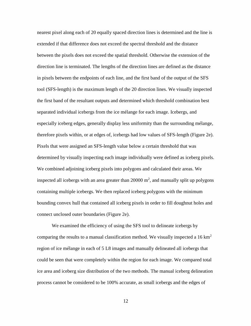
nearest pixel along each of 20 equally spaced direction lines is determined and the line is
extended if that difference does not exceed the spectral threshold and the distance
between the pixels does not exceed the spatial threshold. Otherwise the extension of the
direction line is terminated. The lengths of the direction lines are defined as the distance
in pixels between the endpoints of each line, and the first band of the output of the SFS
tool (SFS-length) is the maximum length of the 20 direction lines. We visually inspected
the first band of the resultant outputs and determined which threshold combination best
separated individual icebergs from the ice mélange for each image. Icebergs, and
especially iceberg edges, generally display less uniformity than the surrounding mélange,
therefore pixels within, or at edges of, icebergs had low values of SFS-length (Figure 2e).
Pixels that were assigned an SFS-length value below a certain threshold that was
determined by visually inspecting each image individually were defined as iceberg pixels.
We combined adjoining iceberg pixels into polygons and calculated their areas. We
inspected all icebergs with an area greater than 20000 m2, and manually split up polygons
containing multiple icebergs. We then replaced iceberg polygons with the minimum
bounding convex hull that contained all iceberg pixels in order to fill doughnut holes and
connect unclosed outer boundaries (Figure 2e).
We examined the efficiency of using the SFS tool to delineate icebergs by
comparing the results to a manual classification method. We visually inspected a 16 km2
region of ice mélange in each of 5 L8 images and manually delineated all icebergs that
could be seen that were completely within the region for each image. We compared total
ice area and iceberg size distribution of the two methods. The manual iceberg delineation
process cannot be considered to be 100% accurate, as small icebergs and the edges of

13
many icebergs often cannot easily be seen in L8 images even with visual inspection.
Therefore, we also inspected and delineated by hand icebergs that could be seen within a
5.4 km2 region of ice mélange from a very-high resolution (0.5 m) Worldview image
from 7/6/16.
Non-iceberg Ice Correction
The thresholding technique used to define ice in L8 images does not differentiate
between icebergs and sea ice or rafts small pieces of ice. Therefore, we quantified the
proportion of total ice delineated by the thresholding technique that was made up of
icebergs in very-high resolution imagery from Worldview satellites. In SF we analyzed
either a 3 km2 region where ice concentrations were high near the ice mélange (images
from 8/21/11 and 6/29/12) or a 12 km2 region where ice concentrations were lower in the
open fjord (images from 7/15/10, 7/11/13, 7/30/13, 8/15/12, and 6/8/15). In RI we
analyzed a 16 km2 region in images from 6/25/13, 7/4/13, 7/17/13, 8/11/13, and 7/19/14,
and in KS we analyzed an 18 km2 region in images from 6/25/13, 7/4/13, and 7/17/13.
We used a thresholding technique as described above to delineate ice polygons, then
visually inspected each ice polygon to determine whether it was an iceberg or other form
of ice (sea ice or conglomeration of brash ice, bergy bits, etc.).
Area – Volume Relationships
We constructed DEMs of icebergs in SF to establish a relationship between
iceberg area and volume. Eight DEMs were generated using very high resolution (~0.5
m) stereo imagery from the Worldview 1 – 3 satellites. We created DEMs using either the
NASA Ames Stereo Pipeline (ASP) (Moratto et al., 2010) or the Surface Extraction with
TIN-based Search-space Minimization (SETSM) (Noh & Howat, 2015) algorithms

14
(Table 2). Comparisons between DEMs generated by the two algorithms revealed
random, non-systematic differences, justifying the merger of the two DEM datasets. All
DEMs have a horizontal resolution of ~2 m and random errors of 3 m (Enderlin &
Hamilton, 2014).
For each DEM we manually created polygon boundaries around icebergs using
ArcMap software. We then found the area and average elevation of each polygon. We
calculate the elevation of the ocean surface by taking the average elevation of at least ten
ice-free pixels dispersed throughout each DEM, and subtracted that elevation from the
mean elevation of pixels making up each iceberg. We multiplied that mean elevation with
the visible area of each iceberg to find its above water volume. Assuming an iceberg
density of 920 kg m-3 and a fjord-water density of 1025 kg m-3, we calculated the
underwater volume and total volume of each iceberg (Figure 3). We then fit all DEM data
using the general power law:
𝑉 = 𝑎𝐴𝑏
where V is the calculated iceberg volume, A is the measured iceberg area, and a and b are
empirically derived constants of best fit.

15
Figure 3: Iceberg areas vs volumes data and fit of data from DEMs. Points are individual
icebergs, and different colors represent different DEMs. The black line is the best fit of
all data, and its equation is displayed.
Iceberg Characteristics and Size Distributions
We used a ranked size distribution of iceberg volumes to quantify the distribution
of iceberg volumes within fjords. For each fjord, we assigned each iceberg a sequential
rank, starting with the lowest volume iceberg as “1”, the second lowest as “2”, and so on
until all icebergs were ranked. When icebergs had identical volumes, they were assigned
a rank equal to the mean of what their ranks would have been had they all been unique
(e.g. if icebergs 3, 4, and 5 all had equal values they would all be assigned the rank of 4).
We observed many small icebergs with identical volumes, so our first rank number was
in the hundreds to thousands. We then tested the fit of several types of distributions
relating individual iceberg volume to the proportion of icebergs with a greater volume in
order to compare observed distributions to previous work and to determine the best fit to
observations.

16
To approximate iceberg depths we used two different shapes to set lower and
upper bounds for classified icebergs. For a minimum depth bound, we use a simple block
type shape in which icebergs maintain the same cross sectional area (A) displayed at the
waterline throughout their depths (d). To calculate a maximum bound we use the lesser of
the height of an inverted elliptical cone with a major axis length (L) equal to the
measured major axis for each iceberg and a minor axis (B) equal to 4𝐴
𝜋𝐿, and 1.43L, which
has been observed as an upper boundary for keel depths relative to lengths (Hotzel &
Miller, 1983; Dowdeswell & Forsberg, 1992). Real, non-tabular icebergs have variable
shapes rather than maintaining a consistent shape throughout their depths or extending to
a pointed cone (Robe, 1980; Barker et al., 2004). Therefore, all real iceberg keel depths
fall somewhere between these two end members. For an iceberg with volume V, area A,
and length L, its depth d is:
𝑉
𝐴 < 𝑑 < {
3𝑉
𝐴
1.43𝐿
As a measure of how variable iceberg sizes are throughout each fjord and between
different regions within each fjord we compare the standard deviation of iceberg areas
within different regions of the fjords for each image. We also compare those values
across different images to identify patterns that are consistent over time for each fjord.
Seasonal Calving Flux
The calving flux represents the amount of ice lost at the terminus through both
iceberg calving and submarine melting over time. To calculate calving fluxes we
multiplied the calving rates by the width and depth of the glacial termini. To determine
calving rates, we average velocity values across the width of each glacier terminus. For

17
each velocity epoch, we calculate the calving rate (c) using the width-averaged terminus
velocity (UM), and the width-averaged change in terminus position (L) between each
velocity epoch:
𝑐 = 𝑈𝑀 − 𝑑𝐿
𝑑𝑡
Velocity data are derived from a combination of radar (Joughin et al., 2010; Joughin et
al., 2011) and optical imagery (Rosenau et al., 2015); terminus position data were semi-
automatically derived using both radar and optical imagery (after Foga et al., 2014). To
determine the seasonal calving rate, we resampled the data to monthly averages before
calculating the calving rate.
Iceberg Trackers
Following methods established by Sutherland et al. (2014) we deployed either
Axonn AXTracker GPS or GeoForce GT1 GPS tracking units from helicopters onto large
(>100 m) icebergs. In SF, 5 trackers were deployed in 2012, 2013, (data presented by
Sutherland et al., 2014), and 2014, and 10 trackers were deployed in 2015. In RI, 3
trackers were deployed in 2013. In KS, 3 trackers were deployed in 2013, and 4 were
deployed in 2014.

18
CHAPTER III
RESULTS
Area-Volume Relationships
We first present the results of creating DEMs and establishing a relationship
between iceberg area and volume to provide necessary context for other results. Iceberg
volume was strongly correlated with cross-sectional area in all eight DEMs generated
using images in SF (Figure 3). Combining data from all DEMs, we found the relationship
between cross-sectional iceberg area (A) at the waterline and iceberg volume (V) to be:
𝑉 = 5.957𝐴1.295
We use this relationship to convert all iceberg areas to volumes for use in further
analyses. Results of fitting power laws of the same form (𝑉 = 𝑎𝐴𝑏) to individual DEMs
resulted in values ranging from 0.94 – 30.09 for the scalar a, and from 1.15 – 1.44 for the
exponent b (Table 2).
Table 2: Coefficients and R2 values for power law fits relating iceberg area to volume
for each DEM created. Date DEM Creation
Algorithm
Number of icebergs
measured
a (±95% confidence
bounds)
b (±95% confidence
bounds)
R2
3/19/11 SETSM 108 30.09 (20.81) 1.15 (0.06) 0.96
8/21/11 ASP 118 17.07 (8.28) 1.18 (0.04) 0.98
8/24/11 ASP 75 0.94 (0.93) 1.44 (0.10) 0.98
6/10/12 ASP 39 1.80 (4.65) 1.39 (0.13) 0.95
6/24/12 SETSM 56 11.21 (22.47) 1.25 (0.09) 0.97
6/29/12 ASP 101 2.95 (2.93) 1.37 (0.08) 0.99
7/31/14 – (1) SETSM 103 2.78 (2.38) 1.33 (0.08) 0.95
7/31/14 – (2) SETSM 112 2.60 (2.27) 1.44 (0.08) 0.95
All Together 712 5.96 (2.59) 1.30 (0.04) 0.92
Fjord Ice Cover
In SF, the total percentage of fjord covered in ice ranged from 2.30 – 33.96%
(Figure 4). Ice covered up to 100% in the mélange that stretches 20 km down-fjord from
the terminus of Helheim Glacier (Figure 4). Other regions of consistently high ice

19
coverage exist around the island at the north end of the fjord and, to a lesser extent, at the
mouth (Figure 5). Beyond the proglacial mélange, ice coverage decreases until reaching a
distance of 50 km from the Helheim terminus. Coverage of ice then remains steady
throughout the remainder of the fjord with the exception of the area near the mouth of the
fjord, where ice from the shelf may be transported into the fjord.
Figure 4: Percentage of fjord surface covered in ice for all images analyzed. Faint lines
represent individual images, and bold lines are averages of all images for each fjord. Data
from SF are blue, RI are red, and KS are green. In RI and KS, dashed lines represent the
northern arms of the fjords, while dotted lines represent the southern arms.
In RI total ice coverage ranged from 1.11 – 23.12% of the fjord surface. Two
regions had ice concentrations higher than in the remainder of the fjord: near the glacier
terminus and in the north arm of the split (Figure 4). Ice concentrations in RI are notably
higher to the north than the south, suggesting that the majority of ice flows outward
through the northern half of the fjord and/or that ice becomes grounded on the shallower
sill there and thus spends more time in that region (Figure 5).

20
KS had less than 2% of its surface covered with ice in all images (Table 1). Ice
coverage was highest near the glacier terminus, and coverage was slightly higher in the
south arm of the fjord than the north (Figure 4, Figure 5).
Figure 5: Probability of ice presence in full fjord images from later than July 15th in RI
(4 images) and KS (7 images) (left panel) and later than July 1st in SF (5 images) (right
panel).
The total amount of ice that we classified and measured as icebergs ranged from
16-99% of the total area of ice coverage (Table 1). Ice that was not classified was either
ice in ice mélange that did not have boundaries that were detected by our method, single
pixels that were above the brightness threshold for ice but were not adjacent to any other
ice pixels, or classified icebergs that were subsequently removed as described below to
account for sea ice captured by our thresholding method.

21
In SF, sea ice made up 42% of the total calculated volume of ice in the image that
we analyzed from June 8, 2015. In all other images sea ice made up an average of 3.31%
(ranging from 0.39 – 9.12%) of the total calculated volume of ice. We therefore removed
L8 images acquired before July of each year. In images from July 1st or later, we used the
“randsample” command in Matlab to remove a random sample of the total set of
delineated icebergs from each of four size classes. We removed 7.88% of icebergs that
are between 0 and 100000 m3, 7.79% of icebergs between 100000 and 200000 m3, 3.64%
of icebergs between 200000 and 300000 m3, and 4.14% of icebergs with volumes greater
than 300000 m3.
In RI, sea ice made up 33.4% and 11.8% of the total calculated volume of ice in
the images that we analyzed from 6/25/13 and 7/4/13, respectively. Sea ice made up an
average of 2.29% (ranging from 0 – 2.73%) of the total calculated volume of ice in Rink
in images from later in the season than July 15. We therefore removed L8 images
acquired before July 15th of each year, and removed a portion of icebergs delineated via
the thresholding technique in L8 images from July 15th or later each year. Because total
ice amounts were lower in RI than in SF we identified sea ice amounts in two rather than
four size classes. We used Matlab to remove 7.44% of icebergs that are between 0 and
300000 m3 and 4.55% of icebergs with volumes greater than 300000 m3. We removed the
same proportion of icebergs in L8 images from KS as total ice amounts in KS were too
low to independently derive robust correction factors from high resolution images there.
We calculated volumes of individual icebergs and the total volume of classified
icebergs present in each image. Total volumes of classified icebergs range from 2.40 –
7.52 km3 (1.22 – 6.77 m3 km-2 and 8.34 – 14.08 m3 km-2 in open fjord and ice mélange,

22
respectively) in SF, 1.04 – 2.04 km3 (0.73 – 5.02 m3 km-2 and 4.11 – 6.61 m3 km-2 in
open fjord and ice mélange, respectively) in RI, and 0.04 – 0.30 km3 (0.10 – 0.81 m3 km-
2) in KS (Table 1, Table 2). In all three fjords, we calculated greater total volumes of ice
in images from earlier in the year (Figure 6). We fit linear regressions to data of ice
volumes versus date, and found the total volume of ice decreases at rates of 0.57 m3 km-2
month-1 in SF between July and late September, and 0.72 m3 km-2 month-1 in RI, and 0.29
m3 km-2 month-1 in KS from mid-July to mid-September.
Figure 6: Calving flux (top panel) and total volume of classified icebergs observed in
each image where the full fjord was visible (lower panel) throughout the year for SF
(blue circles), RI (red squares), and KS (green triangles). Average annual calving fluxes
are shown as dotted lines in the upper panel. Linear regression lines of best fit are shown
on the lower panel and are annotated with their slopes (km3 month-1).
Comparisons to manual classification of ice mélange reveal that the SFS method
that we use tends to split large icebergs into several smaller icebergs (Table 3). We were
unable to use the manual delineation method to define a robust correction factor as the
resolution of L8 images is too low to accurately delineate all icebergs, and especially

23
small icebergs, present in the ice mélange of images. Iceberg volumes reported for areas
of ice mélange are therefore lower bounds on the total ice present in ice mélange areas.
Table 3: Results of classifying 16 km2 of ice mélange automatically and manually in
each of five L8 images and 5.4 km2 manually in one WV image. Number of Icebergs in Size Classes (105 m3) per Area of Ice Mélange
(km2)
n
(km-2)
Iceberg
Vol (105
m3 km-2)
0 – 1
n (%)
1 – 2
n (%)
2 – 3
n (%)
3 – 4
n (%)
4 +
n (%)
Automatic
Classification,
All
29 131 24 (81.0) 2.4 (8.25) 0.89 (3.05) 0.49 (1.68) 1.8 (6.06)
L8 Manual, All 10 173 2.5 (24.9) 1.6 (15.6) 1.3 (12.9) 0.69 (6.88) 4.0 (39.8)
WV Manual,
Single Image
30 473 16 (54.0) 2.6 (8.70) 2.0 (6.83) 0.37 (1.24) 8.7 (29.2)
Individual images
8/7/14
Auto 18 119 14 (80.8) 1.5 (8.54) 0.63 (3.56) 0.31 (1.78) 0.94 (5.34)
Manual 9.6 161 3.0 (31.2) 1.7 (17.5) 1.1 (11.7) 0.75 (7.79) 3.1 (31.8)
7/7/15
Auto 31 60.3 24 (78.9) 2.4 (7.99) 0.88 (2.87) 0.69 (2.25) 2.4 (7.99)
Manual 10 82.0 2.9 (29.2) 1.6 (15.5) 1.2 (11.8) 0.50 (4.97) 3.9 (38.5)
7/16/15
Auto 20 116 15 (76.7) 2.1 (10.5) 0.75 (3.83) 0.31 (1.60) 1.4 (7.35)
Manual 8.5 175 2.3 (26.5) 0.69 (8.09) 1.2 (14.0) 0.38 (4.41) 4.0 (47.1)
9/15/14
Auto 41 145 34 (82.9) 3.5 (8.56) 1.2 (2.91) 0.75 (1.83) 1.6 (3.82)
Manual 13 192 2.9 (23.2) 2.8 (21.7) 1.6 (12.8) 1.0 (7.88) 4.4 (34.5)
9/22/14
Auto 37 198 31 (82.9) 2.5 (6.77) 1.0 (2.71) 0.38 (1.02) 2.4 (6.60)
Manual 9.1 253 1.3 (14.4) 1.1 (12.3) 1.3 (14.4) 0.81 (8.90) 4.6 (50.0)
Iceberg Characteristics
SF had the widest range of iceberg properties seen in the three fjords, with lengths
of individual icebergs ranging from 30 to 2547 m, as well as the lowest average iceberg
size at a length of 66 m. KS had the smallest range of iceberg sizes (lengths 30 – 780 m)
and the smallest maximum iceberg size of the three fjords, but the highest average
iceberg length at 77 m. RI was intermediate in iceberg size range (length 30 – 1959 m),
maximum size, and average length (70 m) (Table 4).

24
Table 4: Iceberg size and depth ranges for all images analyzed of SF, RI, and KS. Fjord SF RI KS
Length Range (Mean) [km] 30 – 2547 (67) 30 – 1959 (70) 30 – 780 (77)
Area Range (Mean) [100 m2] 3 – 40300 (23) 3 – 10300 (30) 3 – 1870 (35)
Volume (Mean) [104 m3] 0.98 – 11724 (22.8) 0.98 – 32585 (48.5) 0.98 – 4002 (50.2)
Maximum Vol. (Mean) [104 m3] 4960 – 28890 (15590) 6650 – 36450 (23740) 598 – 4000 (15520)
Block Depth Range (Mean) [m] 28 – 257 (42) 28 – 300 (43) 28 – 186 (48)
Cone Depth Range (Mean) [m] 45 – 600 (91) 41 – 840 (96) 45 – 250 (107)
L:D Ratio Range (Mean) Blocks 1.06 – 47.4 (1.48) 0.97 – 6.78 (1.51) 0.70 – 5.69 (1.58)
L:D Ratio Range (Mean) Cones 0.70 – 15.8 (0.71) 0.70 – 2.31 (0.71) 0.70 – 3.12 (0.74)
Minimum areas of classified icebergs were bounded by the area of a simplified
polygon incorporating two L8 pixels (304 m2). Individual iceberg areas ranged to 860000
m2 in SF, to 1030000 m2 in RI, and to 187000 m2 in KS. The average area of icebergs in
SF, RI, and KS was 2310, 3030, and 3590 m2, respectively (Table 4).
Iceberg keels depth estimates ranged from 28 – 257 m, 28 – 300 m, and 28 – 186
m in SF, RI, and KS, respectively, for block type icebergs (Table 4). For inverted cones,
maximum depth estimates were truncated at glacial terminus depths (600 m in SF, 840 m
in RI, and 250 m in KS), for 0.037, 0.009, and 8.61% of icebergs in SF, RI, and KS,
respectively. All three fjord had significant proportions (1 – 27% in SF, 2 – 28% in RI,
and 5 – 37% in KS) of icebergs reaching depths greater than 100 m, below which fjord
waters begin to warm (Table 5, Figure 7).
Table 5: Combined number of icebergs (average number per image) reaching depths
greater than 100 m observed in all images for each fjord. Depth (m) SF RI KS
100 1864 – 36058 (266 – 5151) 433 – 6514 (62 – 931) 208 – 1543 (21 – 154)
200 49 – 7898 (7 – 1128) 18 – 1528 (3 – 218) 0 – 549 (0 – 55)
300 1 – 1854 (0 – 265) 1 – 432 (0 – 62) 0 (0)
400 0 – 495 (0 – 71) 0 – 155 (0 – 22) 0 (0)

25
Figure 7: Percentage of icebergs reaching various depths (bars) and typical average
temperature profiles during 3 separate summer seasons (black lines) for SF (left), RI
(center), and KS (right) fjords. Blue bars represent minimum depths (block shape
icebergs) and red bars are maximum depths (cone shaped icebergs). The depth of the
grounding line at KS is shown as a dotted line in the right panel.
Iceberg Size Distributions
By number, all three fjords are dominated by small icebergs, but larger icebergs
account for more of the total volume. The smallest icebergs (< 100000 m3 (~65 m long))
typically make up more than two thirds of the total number of icebergs in all three fjords,
but account for less than 10% of the total ice volume. By contrast, icebergs larger than
107 m3 (~400 m long) account for just 0.28%, 1.41%, and 0.49% of the number of
icebergs but 29.7%, 57.7%, and 14.1% of the total volume in SF, RI, and KS,
respectively (Figure 8).

26
Figure 8: Average (bars) ± one standard deviation (error bars) of the total count (blue)
and total volume (red) of classified icebergs across all images of SF (left), RI (center),
and KS (Right).
Distributions of iceberg sizes have been described using power laws (Tournadre
et al., 2016), Weibull distributions (Savage et al., 2000), and most often lognormal
distribution laws (Wadhams, 1988; Dowdeswell & Forsberg, 1992; Tournadre et al.,
2012, 2016), which have also been used to seed models (Bigg et al., 1997; Mugford &
Dowdeswell, 2010). We examined the ability of the above distribution laws as well as the
generalized Pareto distribution to describe our observations of iceberg volumes. The
generalized Pareto distributions provided the best fit to the data (Figure 9). The survival
function of the generalized Pareto distribution quantifies the probability (P) that the
volume (V) of a randomly selected iceberg will be greater than a volume (v) and is given
by the equation:
𝑃(𝑉 > 𝑣) = (1 +𝜀𝑣
𝜎)
−1𝜀

27
where 𝜎 is the scale parameter and 𝜀 is the shape parameter. Fitting all icebergs from
each fjord to generalized Pareto distributions resulted in values of 39926, 43738, and
51212 for 𝜎 and 0.8670, 1.0194, and 1.2857 for 𝜀 in SF, RI and KS, respectively (Figure
10,
Table 6).
Figure 9: Iceberg volumes versus the probability of a randomly selected iceberg having a
greater volume for icebergs delineated using thresholding in SF (blue circles) and lines of
best fits to data for a power law (green), Pareto distribution (black), lognormal
distribution (red), and Weibull distribution (magenta).
Table 6: Coefficients and goodness of fits for generalized Pareto distributions describing
the probability (P) of a random iceberg having a volume (V) greater than v. Where
P(V>v)=1+(εv/σ)^((-1)/ε)
Fjord Iceberg Delineation Method
(Threshold or SFS) σ (±95% confidence bounds)
ε (±95% confidence
bounds)
SF Threshold 39926 (436) 0.8670 (0.0105)
SFS 36923 (657) 0.9182 (0.0175)
RI Threshold 43738 (1210) 1.0194 (0.0282)
SFS 38151 (1568) 0.7637 (0.0410)
KS Threshold 51212 (3017) 1.2857 (0.0655)

28
Figure 10: Volume distributions. Probability of a random iceberg being greater than a
specified volume for SF (blue), RI (red), and KS (green).
We attempted the same distribution fits as above using iceberg lengths rather than
volumes (Figure 11). Again, a Pareto distribution was best able to describe the data, but
overall the model was not able to predict iceberg lengths as well as volumes. In
particular, the abundance of large icebergs was under predicted by the model using
length.

29
Figure 11: Iceberg lengths versus the probability of a randomly selected iceberg having a
greater length for all icebergs observed in SF (blue circles) and lines of best fits to data
for a power law (green), Pareto distribution (black), lognormal distribution (red), and
Weibull distribution (magenta).
Ice Calving Flux
Ice calving flux is highest in SF (24 km3 yr-1), intermediate in RI (17 km3 yr-1),
and lowest in KS (1.6 km3 yr-1) (Figure 6). In all three fjords, a seasonal signal was
apparent with low or negative (meaning the glacier terminus is advancing without
calving) fluxes throughout the winter, and higher than average calving fluxes occurring in
the summer months, most notably in August. In the spring of both years in SF we
observed one month with a high calving flux during the transition between lower winter
calving rates and higher summer rates (45 km3 yr-1 in March 2013 and 83 km3 yr-1 in
April 2014) (Figure 6).
Iceberg Trackers
Of all 25 trackers placed in SF, 13 transmitted positions throughout the fjord and
eventually exited, five provided records within the fjord but stopped transmitting before
exiting, and seven transmitted very limited or sporadic data that we do not use. Over the

30
entire fjord, the average residence time of icebergs was 132 days. Average residence time
in the proglacial mélange for the 12 icebergs that we tracked there was 70 days, though it
should be noted that we did not track these icebergs starting at Helheim Glacier, but
rather 3 - 15 km down-fjord from the calving face. For the 13 icebergs that traversed the
entire north-south portion of the fjord (beginning 20 km down-fjord from the terminus of
Helheim Glacier) the average residence time in that region was 62 days. We observed
icebergs recirculating primarily in two regions in SF: in the broad region between 35 and
55 km down-fjord of Helheim Glacier’s terminus, where icebergs spent an average of 34
days, and in the region between the two constrictions from 64 to 86 km down-fjord from
the Helheim Glacier, where icebergs spent an average of 23 days (Figure 12). Outside of
the ice mélange, down-fjord motion was generally seen on the right (western) side of the
fjord, while toward glacier motion was seen on the left (eastern) side.

31
Figure 12: Example GPS tracker paths from RI and KS overlain on a L8 image from
7/8/14 (left), and from SF overlain on a L8 image from 8/7/14 (right).
In RI, two of the trackers that were placed on icebergs traversed the entire fjord
and exited via the northern arm, while the third was lost after just two days. Residence
times of the two tracked icebergs were 24 and 103 days. Both icebergs recirculated in the
region between the glacier terminus and 16 km down-fjord of the terminus, spending 13
and 8 days there. One of the icebergs, UO07, subsequently exited 11 days after leaving
that area, while the other, UO14, recirculated for 44 days in the broad region between 35
and 64 km down-fjord from the terminus before spending 51 days in the north arm of the
fjord where it was likely grounded on the shallow (~240 m) sill, and eventually exiting
(Figure 12). We observed UO14 in a Worldview 2 image from 9/16/13, and measured its

32
area to be 30913 m2 and its length to be 300 m. Using these measurements we calculated
the keel depth of the iceberg to be 126 – 377 m, confirming its potential to ground on the
northern sill. For both icebergs, motion away from the fjord generally occurred on the
right hand (northern) side of the fjord, while toward glacier motion occurred on the left
hand (southern) side.
In KS, two icebergs that were tracked in 2013 traversed through the entire fjord
and exited the north arm after 11 and 21 days. A third tracker only transmitted limited
data for two days. In 2014 four trackers were deployed, one of which only transmitted
data for two days so its data are not included. The three icebergs that were tracked all
recirculated in the region between KS glacier and 20 km down-fjord, spending 17, 64,
and >35 (the tracker that was in the zone for 35 days stopped transmitting before leaving
the area) days there. Two of the icebergs then traveled down-fjord and one entered the
southern arm of the fjord after five days, then stopped transmitting, while the other
recirculated in the region between 20 and 30 km down-fjord for 20 days before entering
the south arm and stopping transmissions 8 days later (Figure 12). Similar to SF and RI,
down-fjord motion was generally observed on the right (northern) side of the fjord, and
toward glacier motion was observed on the left (southern) side.

33
CHAPTER IV
DISCUSSION
Fjord Ice Volumes
Quantifying the volume of ice that resides within, and transports through, a fjord
is essential to quantifying the GrIS freshwater flux and its influence on fjord and shelf
water properties. In situ measurements of iceberg depths are difficult to obtain because
icebergs can damage or destroy moorings and present hazards that preclude
oceanographic vessels from a near approach. Even when those hazards are mitigated, any
in situ measurements of depth are necessarily limited to small spatial scales (e.g. Andres
et al., 2015) relative to what we can observe on the surface with satellite or aerial
imagery. Establishing a relationship between iceberg areas visible in satellite or areal
images and iceberg volumes is a solution that allows us to quantify volumes and depths
of large numbers of icebergs.
We used an area to volume conversion as area is the property of icebergs that we
directly measure that provides the greatest amount of information about iceberg size. To
compare results to other studies, however, we also fit an empirical relationship between
iceberg length (L) in meters and mass (M) in tonnes for 712 icebergs using the power
law:
𝑀 = 𝑎𝐿𝑏
In our relationship, a=2.35, b=2.55, and the correlation coefficient R2 = 0.93. These
results are similar to those of Hotzel & Miller, (1983) (a = 2.009, b = 2.68, R2= 0.90)
who used 168 icebergs observed off Labrador, and Barker et al. (2004) (a = 0.43, b =

34
2.9, R2 = 0.92) who used 14 measurements of 9 icebergs observed in waters around
Labrador by Smith & Donaldson, (1987). These similarities suggest a robust relationship
that can be applied to icebergs produced by calving glaciers in other Arctic regions.
The amount of ice per surface area of fjord water decreases in all three fjords
between spring and late summer (Figure 6). Decreases in ice coverage could be the result
of decreased input from calving glaciers, increases in ice export out of fjords, and/or
increased melt of icebergs and sea ice within fjords. We rule out decreased calving fluxes
as we observed calving to be steady or increase over the same time period in each fjord
(Figure 6). Reductions in sea ice are also unable to account for the observed decrease in
ice volume. Analysis of WV images show that the contribution of sea ice to total ice
amount decreased by 1.39% between July and late August in SF, and 1.91% per month
between mid-July and mid-August in RI. Total ice volumes calculated from L8 images
decreased by 10 – 20% over the same timeframe. Increases in export and melting likely
both contribute to decreased total iceberg volume. In the winter, sea ice forms in RI and
KS as well as outside of all three fjords, effectively blocking export of icebergs from the
fjords and leading to a buildup of icebergs which reaches a maximum in the early spring.
Break up of sea ice in the late spring and summer allows the buildup of ice to be cleared
resulting in a decrease in total ice volume. Additionally, freshwater runoff from the GrIS
increases in summer causing stronger net down-fjord flow (Bamber et al., 2012; Polar,
2013; Bartholomaus et al., 2016). Increased runoff may also cause higher rates of iceberg
melt, as runoff can take the form of subsurface plumes with positive temperature
anomalies that flow down-fjord at depths containing iceberg keels (Carroll et al., 2015;
Cowton et al, 2015).

35
Using standard residence time calculations, we can also obtain first order
approximations of ice fluxes using our measurements of total ice volume and tracked
iceberg residence times. Using the equation:
𝐼𝑐𝑒 𝐹𝑙𝑢𝑥 = 𝑇𝑜𝑡𝑎𝑙 𝐼𝑐𝑒 𝑉𝑜𝑙𝑢𝑚𝑒
𝐼𝑐𝑒 𝑅𝑒𝑠𝑖𝑑𝑒𝑛𝑐𝑒 𝑇𝑖𝑚𝑒
and average total ice volumes and residence times for each fjord we estimate ice fluxes of
18, 9.6, and 2.5 km3 yr-1 for SF, RI, and KS respectively. These estimates compare
favorably to measured ice fluxes of 24, 17, and 1.6 km3 yr-1, and demonstrate that we can
obtain reasonable estimates of either ice flux, volume, or residence time if data for the
other two properties are available.
Iceberg Classification
While our method is able to quantify many of the icebergs seen in L8 images, we
cannot classify all ice for two primary reasons: the difficulty of finding and connecting
discrete edges of icebergs within ice mélange, and to a lesser extent the exclusion of very
small bits of ice that occupy a single pixel or less of the images.
Ice mélange is most prevalent in SF where a persistent proglacial mélange exists
in all available images, typically occupying the majority of the section of fjord running
east from the terminus of Helheim Glacier for 20 km. In the images available for this
study, we classified between 4.7 and 38.6% of the total ice area in the mélange as
icebergs. Despite the fact that our method splits up some large icebergs, we observe a
larger average area of icebergs in the ice mélange (3580 m2) compared with those in the
remainder of the fjord (2150 m2). Icebergs deteriorate through mechanical breakup and
melt within fjords, so the largest icebergs will typically be found near parent glaciers that
supply them to fjords (Kubat et al., 2007; Enderlin & Hamilton, 2014; Wagner et al.,

36
2014). Additionally ice mélange has been shown to exert a back-stress sufficient to
prevent calving from glacier termini, and similar processes may prevent the breakup of
large icebergs in mélange (Amundson et al., 2010).
The volume of icebergs delineated by our automated classification process is on
average 76% of the volume delineated manually, and not all ice in ice mélange is
classified as part of an iceberg (Figure 2). In the DEMs used for area-volume
relationships, ice in mélange that was not part of large icebergs generally had a freeboard
height of less than 1 m. We therefore use a total thickness of 10 m for unclassified ice as
an upper bound and calculate a volume of ice based on that thickness for unclassified ice
in ice mélange. To estimate the volume of ice unaccounted for by the misclassification of
large icebergs as smaller icebergs, we assume that the calculated volume of classified
icebergs is 76% of the actual volume of those icebergs. Under these assumptions, we
estimate that we are able to classify an average of 48% of the total ice mélange volume as
icebergs (Table 7). This is likely to be an underestimate, as much of the ice in ice
mélange is thin bergy bits and brash ice that has a thickness of less than 10 m.
Table 7: Estimated volumes of ice mélange that was not classified as icebergs in SF. Date Total Classified Ice
Mélange Volume
(km3)
Volume Missing From
Misclassifying Large
Icebergs (km3)
Unclassified Mélange
Volume Assuming
Average Non-Iceberg
Ice Thickness of 10 m
(km3)
Percent of Total Ice
Mélange Volume
Classified as Icebergs
8/7/2014 1.18 0.38 1.32 41
9/15/2014 3.70 1.19 2.46 50
9/22/14 2.75 0.88 2.31 46
7/7/2015 2.03 0.65 1.27 51
7/16/2015 3.36 1.08 2.57 48
Growlers, bergy bits, and brash ice, collectively defined as pieces of ice smaller
than 15 m in length (Canadian Ice Service, 2005), account for a portion of total ice area
found using the threshold method that we did not include in our iceberg analyses. The

37
area of this small ice that was removed ranged from 0.3 – 1.5%, 0.3 – 5.6%, and 0.8 –
3.8% of the total ice area in images from SF, RI, and KS respectively (Table 1). Even if
we assume a generous average depth of 10 m for these small bits of ice, the volume of
this removed ice is below 1% of the calculated volume of classified icebergs in all
images.
Iceberg Distribution
Variability in iceberg size distributions is greater between the three fjords than
within any one fjord, suggesting that differences in total ice discharge, calving styles, and
grounding line depths account for differences in iceberg properties rather than seasonal
effects or geographic features.
The smallest average iceberg size, and therefore the lowest values of the scale and
shape parameters for generalized Pareto distributions, were observed in SF (
Table 6, Figure 13). Calving from Helheim Glacier is dominated by large scale
calving events over its entire depth (~600 m) in which buoyant forces lift the terminus,
which may be held below flotation by its attachment to the rest of the glacier, and cause
icebergs to calve with a bottom out rotation (James et al., 2014; Murray et al., 2015). This
calving style causes ice to rise quickly into a tightly packed mélange where collision with
other ice is likely. Continued collisions and friction between icebergs transiting the
mélange may be responsible for additional breakdown of large icebergs into smaller
pieces. Icebergs also move slowly through the mélange, spending more than 70 days
there on average, allowing time for melting. The highest water temperatures of the three
fjords is observed in SF (ranging from near 0° C near the surface up to 4.5° C at >400 m

38
depth (Figure 7)), and continued melting of transiting and circulating icebergs may also
contribute to the lower average size of icebergs in the fjord (Straneo et al., 2010;
Bartholomaus et al., 2016).
Figure 13: Parameters of generalized Pareto distributions for all images analyzed in SF
(blue circles), RI (red squares) and KS (green triangles). Parameters from distributions
describing icebergs found using the threshold method are represented by closed symbols,
and those using the SFS method are represented by open symbols.
Iceberg mean sizes and parameters of generalized Pareto distributions from RI are
intermediate of the three fjords observed (
Table 6, Figure 13). Additionally, iceberg sizes vary to a greater degree
throughout RI than in either SF or KS (Figure 14). Calving of RI occurs by two separate
processes: small scale events that occur with high frequency and lead to detachment of
non-tabular icebergs, most frequently from crevassed areas of the glacier as weak points
in the glacier associated with those crevasses fail; and large scale events in which large
tabular icebergs calve from the least crevassed portion of the glacier as buoyant forces act
on portions of the glacier that are held below flotation and cause fracturing (Medrzycka et

39
al., 2016). While the second mechanism is similar to the dominant style of calving in SF,
icebergs calved in this manner in RI do not regularly roll as they calve, and generally do
not calve into an existing compact ice mélange in summer. Icebergs in RI may therefore
be subject to less breakdown via collisions and grinding against other icebergs. We do
observe an ephemeral ice mélange in RI when, after a large calving event, a large
grouping of ice travels down-fjord staying in close proximity, potentially enhancing
breakdown via collision.
In RI, high concentrations of ice occur near the head of the fjord, throughout the
north section of the narrow section of the fjord, and behind the sill north of the island
(Figure 5). High concentrations to the north may indicate the influence of rotation on
surface and subsurface waters flowing down-fjord which is also suggested by the
trajectories of tracked icebergs (Figure 12). High ice concentrations to the north of the
island are likely the result of larger icebergs reaching depths exceeding the depth of the
sill and becoming grounded, as did one of the icebergs that we tracked. Notably, we
observed that the temporal variability in iceberg areas decreased with increasing distance
from the glacier terminus (Figure 14). We attribute this decrease in variability to the
fracture of the largest icebergs as they traverse the fjord which results in more uniform
pieces of ice with distance from the glacier terminus.
Total ice coverage in KS is too low to reveal any strong spatial or temporal
patterns, but comparisons to RI and SF do reveal interesting contrasts. In KS, variability
in iceberg areas, which we approximate using the standard deviation of iceberg areas, is
the lowest of the three fjords, and most consistent throughout the fjord (Figure 14). The
average iceberg area is largest in KS despite the glacier having the shallowest grounding

40
line of the three. We attribute the consistency and larger size to a less violent style of
calving where ice is not rolling and rising from great depths and therefore remains more
intact. The low concentrations of ice also allow less chance of icebergs grinding or
knocking together and subsequently breaking into smaller pieces. Water in KS is also
colder at equivalent depths than in SF or RI leading to less melting (Figure 7). Finally,
though our data are limited, residence times may be lowest of the three fjords in KS,
allowing less time for iceberg deterioration during transit through the fjord.
Figure 14: Iceberg size variability and down-fjord speed in geographic zones in SF (left),
RI (center), and KS (right). Standard deviation of iceberg areas is displayed for each
image (black circles), and the average standard deviation is shown (black squares).
Average iceberg area is shown (black dotted line) for reference. Red triangles represent
average down-fjord speed of tracked icebergs in each zone. Red error bars are ±1
standard diviation in SF and KS, and represent the range of values in RI where data
consists of 2 icebergs only. No tracked icebergs traversed the southern arms of RI or KS,
hence no data is presented for iceberg speeds in those zones.
Keel Depths and Melt
Icebergs reaching deeper, warmer fjord waters have the greatest potential to affect
water properties because of both their direct contribution of freshwater and their ability to

41
entrain ambient deep water as the buoyant melt rises upwards through the water column.
The melting of icebergs is analogous to the subaqueous melting of glacial termini which
has been investigated using observations, numerical modeling, and laboratory
experiments (Eijpen et al., 2003; Rignot et al., 2010; Xu et al., 2012).
We calculated the total surface area of icebergs at different depths based on block
shaped icebergs. This approach may overestimate surface area as real icebergs are likely
to have a shape that tapers with depth rather than maintaining a constant horizontal cross
section. Our estimates of submerged surface area of icebergs exceeds that of the glacier
faces throughout all three fjords (
Table 8).
Icebergs have the greatest potential to influence water properties in SF because of
the high concentration of icebergs and relatively high water temperature. Water
temperature in SF increases below the surface layer, reaching temperatures of 2°C at
200m and rising to 3.5°C at 400m (Figure 7) (Sutherland et al. 2014). Enderlin &
Hamilton (2014) calculated an average iceberg melt rate of ~0.39 m d-1 in SF. Applying
that melt rate to the total surface area of submerged icebergs in SF yields a freshwater
contribution from iceberg melt of 0.083 km3 d-1 to the fjord. This melt rate may be an
upper bound on summer melt, but is unrealistic as a year round estimate as it would
imply a total freshwater input from iceberg melt of 30 km3 yr-1, which is higher than our
measured annual ice flux of 24 km3 yr-1. The discrepancy may in part be due to small
icebergs which likely experience less overall melt, as their keels remain in the upper
portion of the water column where temperatures are low. Applying the average melt rate
to only the surface area of icebergs below 100 m, where water temperatures begin to

42
increase, yields a freshwater input from iceberg melt of 0.009 km3 d-1, which could be
considered a lower bound on freshwater input from iceberg melt. This is still greater than
the 0.006 km3 d-1 of freshwater from melting of the glacier face, based on a submarine
melt rate of 1.78 m d-1 derived by Sutherland & Straneo (2012), though the input of
freshwater from iceberg melt is distributed throughout the fjord rather than concentrated
in one spot as is the input from submarine glacial melt.
Table 8: Water temperature and average surface area (km2) of ice at depth. Temperatures
are averages of measurements taken throughout each fjord over three summers. Iceberg
areas assume that icebergs maintain their cross-sectional area at the water line throughout
their depths. Depth (m) 0-100 100-200 200-300 300-400 400+
SF Mean Temp. (°C) 1.03 1.91 2.93 3.62 3.95
Glacier Face 0.55 0.55 0.55 0.55 1.1
Icebergs 188 21.9 2.86 0 0
RI Mean Temp. (°C) 1.41 1.84 2.07 2.28 2.75
Glacier Face 0.47 0.47 0.47 0.47 2.1
Icebergs 34.1 5.90 1.20 0.14 0
KS Mean Temp. (°C) 0.62 1.07 1.89 - -
Glacier Face 0.42 0.42 0.21 - -
Icebergs 6.29 1.28 0 - -

43
CHAPTER V
CONCLUSIONS
Icebergs are a significant component of total freshwater discharge from the GrIS.
We are able to use available satellite data to quantify distributions of iceberg sizes and
total coverage of fjords by icebergs. Additionally, by using high resolution satellite
imagery to construct DEM’s we created a robust relationship between iceberg areas and
volumes, and used that relationship to quantify the total volume of ice present in fjords
and to estimate iceberg keel depths and subsurface iceberg surface area.
We found substantial differences in iceberg characteristics between the three
fjords that we investigated. Differences in icebergs are tied to differences in glacier
grounding line depths, calving styles, and fjord water properties and circulation. We
determined that iceberg size distributions follow generalized Pareto distributions, and we
recommend using Pareto laws when determining iceberg size distributions to seed
models.
This work represents first steps towards quantifying iceberg properties on a large
scale and quantifying freshwater input from iceberg melt. Future study includes applying
these methods to other fjords, exploring the use of radar rather than optical satellite
observations to obtain year-round coverage, using these distributions to seed icebergs in
numerical ocean models, and refining estimates of iceberg keel depths, subaqueous
surface areas, and freshwater input from iceberg melt. This work highlights the need for
more observations of iceberg keel shapes and depths. Expanding records of surface

44
currents through continued use of icebergs as drifters or other means, as well as obtaining
measurements of water properties and circulation within other fjords is also necessary to
continue and expand this work.

45
REFERENCES CITED
Amundson, J. M., Fahnestock, M., Truffer, M., Brown, J., Lüthi, M. P., & Motyka, R. J.
(2010). Ice mélange dynamics and implications for terminus stability, Jakobshavn
Isbrse, Greenland. Journal of Geophysical Research: Earth Surface, 115(1), 1–12.
http://doi.org/10.1029/2009JF001405
Andres, M., Silvano, A., Straneo, F., & Watts, D. R. (2015). Icebergs and Sea Ice
Detected with Inverted Echo Sounders. Journal of Atmospheric and Oceanic
Technology, 32(5), 1042–1057. http://doi.org/10.1175/JTECH-D-14-00161.1
Azetsu-Scott, K., & Syvitski, J. P. M. (1999). Influence of melting icebergs on
distribution, characteristics and transport of marine particles in an East Greenland
fjord. Journal of Geophysical Research, 104(C3), 5321.
http://doi.org/10.1029/1998JC900083
Bamber, J., Broeke, M. Van Den, Ettema, J., Lenaerts, J., & Rignot, E. (2012). Recent
large increases in freshwater fluxes from Greenland into the North Atlantic.
Geophysical Research Letters, 39, 8–11. http://doi.org/10.1029/2012GL052552
Barker, A., Sayed, M., & Carrieres, T. (2004). Determination of Iceberg Draft , Mass and
Cross- Sectional Areas NRC Publications Archive ( NPArC ). Proceedings of The
Fourteenth International Offshore and Polar Engineering Conference, (January).
Bartholomaus, T. C., Stearns, L. A., Sutherland, D. A., Shroyer, E. L., Nash, J. D.,
Walker, R., … Broeke, M. Van Den. (2016). Contrasts in the response of adjacent
fjords and glaciers to ice-sheet surface melt in West Greenland. Annals of
Glaciology. http://doi.org/10.1017/aog.2016.19
Bigg, G. R., & Nicholls, K. W. (2001). Iceberg trajectory modeling and meltwater
injection. Journal of Geophysical Research, 106(C9), 19903 – 19915.
Bigg, G. R., Wadley, M. R., Stevens, D. P., & Johnson, J. A. (1997). Modelling the
dynamics and thermodynamics of icebergs. Cold Regions Science and Technology,
26, 113–135.
Bigg, G. R., & Wilton, J. (2013). Iceberg risk in the Titanic year of 1912 : was it
exceptional? Weather, 69(4), 100 – 104.
Box, J., & Colgan, W. (2013). Greenland Ice Sheet Mass Balance Reconstruction . Part
III : Marine Ice Loss and Total Mass Balance ( 1840 – 2010 ). Journal of Climate,
26, 6990–7002. http://doi.org/10.1175/JCLI-D-12-00546.1
Canadian Ice Service. (2005). Manual of Standard Proceedures for Observing and
Reporting Ice Conditions. (D. Fequet, Ed.) (Revised 9t). Ottawa, Ontario:
Environment Canada.

46
Carroll, D., Sutherland, D. A., Shroyer, E. L., Nash, J. D., Catania, G. A., & Stearns, L.
A. (2015). Modeling Turbulent Subglacial Meltwater Plumes : Implications for
Fjord-Scale Buoyancy-Driven Circulation. Journal of Physical Oceanography, 45,
2169–2185. http://doi.org/10.1175/JPO-D-15-0033.1
Cowton, T., Slater, D., Sole, A., Goldberg, D., & Niewnow, P. (2015). Modeling the
impact of glacial runoff on fjord circulation and submarine melt rate using a new
subgrid-scale parameterisization for glacial plumes. Journal of Geophysical
Research: Oceans, 120, 796–812. http://doi.org/10.1002/2014JC010324.Received
Crocker, G. B. (1993). Size distributions of bergy bits and growlers calved from
deteriorating icebergs. Cold Regions Science and Technology, 22, 113–119.
Death, R., Siegert, M. J., Bigg, G. R., & Wadley, M. R. (2006). Modelling iceberg
trajectories , sedimentation rates and meltwater input to the ocean from the Eurasian
Ice Sheet at the Last Glacial Maximum. Palaeogography, Palaeoclimatology,
Palaeoecology, 236, 135–150. http://doi.org/10.1016/j.palaeo.2005.11.040
Dowdeswell, J. A., & Dowdeswell, E. K. (1989). Debris in Icebergs and Rates of Glaci-
Marine Sedimentation : Observations from Spitsbergen and a Simple Model. The
Journal of Geology, 97(2), 221–231.
Dowdeswell, J. A., & Forsberg, C. F. (1992). The size and frequency of icebergs and
bergy bits derived from tidewater glaciers in Kongsfjorden , northwest Spitsbergen.
Polar Research, 11(2), 81–91.
Eijpen, K. J., Warren, C. R., & Benn, D. I. (2003). Subaqueous melt rates at calving
termini : a laboratory approach. Annals of Glaciology, 36, 179 – 183.
Enderlin, E. M., & Hamilton, G. S. (2014). Estimates of iceberg submarine melting from
high-resolution digital elevation models: application to Sermilik Fjord, East
Greenland. Journal of Glaciology, 60(224), 1084–1092.
http://doi.org/10.3189/2014JoG14J085
Enderlin, E. M., Howat, I. M., Jeong, S., Noh, M.-J., van Angelen, J. H., & van den
Broeke, M. R. (2014). An improved mass budget for the Greenland ice sheet.
Geophysical Research Letters, 41, 866–872.
http://doi.org/10.1002/2013GL059010.Received
Fichefet, T., Poncin, C., Goosse, H., Huybrechts, P., Janssens, I., & Le Treut, H. (2003).
Implications of changes in freshwater flux from the Greenland ice sheet for the
climate of the 21st century. Geophysical Research Letters, 30(17), 1911–1915.
http://doi.org/10.1029/2003GL017826
Foga, S., Stearns, L. A., & van der Veen, C. J. (2014). Using satellite remote sensing data
to determine terminus and ice melange variability at Helheim Glacier, East
Greenland. Marine Technology Society Journal (Polar Instruments and Methods).
http://doi.org/10.4013/MTSJ.48.5.3

47
Grobe, B. H. (1987). A Simple Method for the Determination of Ice-Rafted Debris in
Sediment Cores. Polargorschung, 57(3), 123–126.
Hotzel, I. S., & Miller, J. D. (1983). ICEBERGS : THEIR PHYSICAL DIMENSIONS
AND THE PRESENTATION AND APPLICATION OF. Annals of Glaciology, 4,
116–123.
Huang, X., Zhang, L., & Li, P. (2007). Classification and Extraction of Spatial Features
in Urban Areas Using High-Resolution Multispectral Imagery. IEEE Geoscience
and Remote Sensing Letters, 4(2), 260–264.
James, T. D., Murray, T., Selmes, N., Scharrer, K., & Leary, M. O. (2014). Buoyant
flexure and basal crevassing in dynamic mass loss at Helheim Glacier. Nature
Geoscience, 7, 593–596. http://doi.org/10.1038/NGEO2204
Joughin, I., Howat, I. M., Smith, B., & Scambos, T. (2011). MEaSUREs Greenland Ice
Velocity: Selected Glacier Site Velocity Maps from InSAR, Version 1. Boulder, CO
USA.
Joughin, I., Smith, B., Howat, I. M., Scambos, T., & Moon, T. (2010). Greenland Flow
Variability from Ice-Sheet-Wide Velocity Mapping. Journal of Glaciology, 56, 415–
430. http://doi.org/http://dx.doi.org/10.3189/002214310792447734
Kubat, I., Sayed, M., Savage, S. B., Carrieres, T., & Crocker, G. B. (2007). An
Operational Iceberg Deterioration Model. Proceedings of the Seventeenth
International Offshore and Polar Engineering Conference, 652–657.
Larsen, P., Overgaard Hansen, M., Buus-hinkler, J., Krane, K. H., & Sønderskov, C.
(2015). Field tracking ( GPS ) of ten icebergs in eastern Baffin Bay , offshore
Upernavik , northwest Greenland. Journal of Glaciology, 61(227), 421–437.
http://doi.org/10.3189/2015JoG14J216
Levine, R. C., & Bigg, G. R. (2008). Sensitivity of the glacial ocean to Heinrich events
from different iceberg sources , as modeled by a coupled atmosphere-iceberg-ocean
model. Paleoceanography, 23, 1–16. http://doi.org/10.1029/2008PA001613
Martin, T., & Adcroft, a. (2010). Parameterizing the fresh-water flux from land ice to
ocean with interactive icebergs in a coupled climate model. Ocean Modelling, 34(3-
4), 111–124. http://doi.org/10.1016/j.ocemod.2010.05.001
Medrzycka, D., Benn, D. I., Box, J. E., Copland, L., Balog, J., Medrzycka, D., … Balog,
J. (2016). Calving behavior at Rink Isbræ , West Greenland , from time-lapse
photos. Arctic, Antarctic, and Alpine Research, 48(2), 263–277.
Moon, T., Joughin, I., Smith, B., & Howat, I. (2012). 21st-Century Evolution of
Greenland Outlet Glacier Velocities. Science, 336, 576–579.

48
Moratto, S. Z. M., Broxton, M. J., Beyer, R. A., Lundy, M., & Husmann, K. (2010).
Ames Stereo Pipeline , NASA ’ s Open Source Automated Stereogrammetry, 1–2.
Mugford, R. I., & Dowdeswell, J. A. (2010). Modeling iceberg rafted sedimentation in
high latitude fjord environments. Journal of Geophysical Research, 115(March), 1–
21. http://doi.org/10.1029/2009JF001564
Murray, T., Selmes, N., James, T. D., Edwards, S., Martin, I., Timothy, O., … Baugé, T.
(2015). Dynamics of glacier calving at the ungrounded margin of Helheim Glacier,
southeast Greenland. Journal of Geophysical Research : Earth Surface, 120, 964–
982. http://doi.org/10.1002/2015JF003531.Received
Neshyba, S. (1980). On the size distribution of Antarctic icebergs. Cold Regions Science
and Technology, 1, 241–248.
Noh, M.-J., & Howat, I. M. (2015). Automated stereo-photogrammetric DEM generation
at high latitudes: Surface Extraction with TIN-based Search-space Minimization
(SETSM) validation and demonstration over glaciated regions. GIScience & Remote
Sensing, 52(2), 198–217. http://doi.org/10.1080/15481603.2015.1008621
Raiswell, R., Tranter, M., Benning, L. G., Siegert, M., De, R., Huybrechts, P., & Payne,
T. (2006). Contributions from glacially derived sediment to the global iron (
oxyhydr ) oxide cycle : Implications for iron delivery to the oceans. Geochimica et
Cosmochimica Acta, 70, 2765–2780. http://doi.org/10.1016/j.gca.2005.12.027
Rignot, E., Fenty, I., Xu, Y., Cai, C., Velicogna, I., Cofaigh, C. Ó., … Duncan, D. (2016).
Bathymetry data reveal glaciers vulnerable to ice-ocean interaction in Uummannaq
and Vaigat glacial fjords , west Greenland. Geophysical Research Letters, 43, 2667–
2674. http://doi.org/10.1002/2016GL067832.Received
Rignot, E., Koppes, M., & Velicogna, I. (2010). Rapid submarine melting of the calving
faces of West Greenland glaciers. Nature Geoscience, 3(3), 187–191.
http://doi.org/10.1038/ngeo765
Robe, R. Q. (1980). Iceberg Drift and Deterioration. In S. C. Colbeck (Ed.), Dynamics of
Snow and Ice Masses (pp. 211 – 259). New York, NY: Academic Press, INC.
Rosenau, R., Scheinert, M., & Dietrich, R. (2015). A processing system to monitor
Greenland outlet glacier velocity variations at decadal and seasonal time scales
utilizing the Landsat imagery. Remote Sensing of the Environment, 169, 1–19.
Savage, S. B., Crocker, G. B., Sayed, M., & Carrieres, T. (2000). Size distributions of
small ice pieces calved from icebergs. Cold Regions Science and Technology, 31,
163–172.
Smith, S. D., & Donaldson, N. R. (1987). Dynamic modelling of iceberg drift using
current profiles. Canadian Technical Report of Hydrography and Ocean Sciences,
(91).

49
Stouffer, R. J., Yin, J., Gregory, J. M., Dixon, K. W., Spelman, M. J., Hurlin, W., …
Weber, S. L. (2006). Investigating the Causes of the Response of the Thermohaline
Circulation to Past and Future Climate Changes. Journal of Climate, 19(8), 1365–
1387. http://doi.org/10.1175/JCLI3689.1
Straneo, F., Hamilton, G. S., Sutherland, D. A., Stearns, L. A., Davidson, F., Hammill,
M. O., … Rosing-asvid, A. (2010). Rapid circulation of warm subtropical waters in
a major glacial fjord in East Greenland. Nature Geoscience, 3(3), 182–186.
http://doi.org/10.1038/ngeo764
Sutherland, D. A., Roth, G. E., Hamilton, G. S., Mernild, S. H., Stearns, L. A., & Straneo,
F. (2014). Quantifying flow regimes in a Greenland glacial fjord using iceberg
drifters. Geophysical Research Letters, 41(23), 8411–8420.
Sutherland, D. A., & Straneo, F. (2012). Estimating ocean heat transports and submarine
melt rates in Sermilik Fjord , Greenland , using lowered acoustic Doppler current
profiler ( LADCP ) velocity profiles. Annals of Glaciology, 53(60), 50–58.
http://doi.org/10.3189/2012AoG60A050
Sutherland, D. A., Straneo, F., & Pickart, R. S. (2014). Characteristics and dynamics of
twomajor Greenland glacial fjords. Journal of Geophysical Research: Oceans, 119,
3767–3791. http://doi.org/10.1002/2013JC009786.Received
Syvitski, J. P. M., Andrews, J. T., & Dowdeswell, J. A. (1996). Sediment deposition in an
iceberg-dominated glacimarine environment , East Greenland : basin fill
implications. Global and Planetary Change, 12, 251–270.
Tournadre, J., Bouhier, N., Girard-Ardhuin, F., & Rémy, F. (2016). Antarctic icebergs
distributions 1992-2014. Journal of Geophysical Research: Oceans, 121, 327–349.
http://doi.org/10.1002/2015JC011178
Tournadre, J., Girard-Ardhuin, F., & Legrésy, B. (2012). Antarctic icebergs distributions,
2002-2010. Journal of Geophysical Research: Oceans, 117(5), 2002–2010.
http://doi.org/10.1029/2011JC007441
USGS. (2016). Lansat 8 (L8) Data Users Handbook. U.S. Geological Survey.
van den Broeke, M., Bamber, J., Ettema, J., Rignot, E., Schrama, E., Berg, W. J. Van De,
… Wouters, B. (2009). Partitioning Recent Greenland Mass Loss. Science, 326,
984–986. http://doi.org/10.1126/science.1178176
Velicogna, I., Sutterley, T. C., & Broeke, M. R. Van Den. (2014). Regional acceleration
in ice mass loss from Greenland and Antarctica using GRACE time-variable gravity
data. Geophysical Research Letters, 41, 8130–8137.
http://doi.org/10.1002/2014GL061052.Received
Wadhams, P. (1988). Winter Observations of Iceberg Frequencies and Sizes in the South.
Journal of Geophysical Research, 93(C4), 3583–3590.

50
Wagner, T. J. W., Wadhams, P., Bates, R., Elosegui, P., Stern, A., Vella, D., … Nicholls,
K. W. (2014). The “ footloose ” mechanism : Iceberg decay from hydrostatic
stresses. Geophysical Research Letters, 41, 5522–5529.
http://doi.org/10.1002/2014GL060832.We
Williams, R., & Macdonald, M. (1995). An image segmentation technique to infer the
outlines of icebergs, depicted in satellite images, from their shadows and bright
sunlit surfaces. Proceedings of the Third Australian and New Zealand Conference
on Intelligent Information Systems, 76–81.
Xu, Y., Rignot, E., Menemenlis, D., & Koppes, M. (2012). Numerical experiments on
subaqueous melting of Greenland tidewater glaciers in response to ocean warming
and enhanced subglacial discharge. Annals of Glaciology, 53(60), 229–234.
http://doi.org/10.3189/2012AoG60A139
Yang, Q., Dixon, T. H., Myers, P. G., Bonin, J., Chambers, D., & Broeke, M. R. Van
Den. (2016). Labrador Sea convection and Atlantic overturning circulation. Nature
Communications, 7, 1–7. http://doi.org/10.1038/ncomms10525