Comparative Analysis of Linear and Non-linear

Extended State Observer

with Application to Motion Control

Kaliprasad A. Mahapatro Ashitosh D. Chavan

Department of Electronics and Telecommunication Department of Electronics and Telecommunication

Vishwakarma Institute of Technology,Pune University MIT Academy of Engineering, Pune University

Pune, Maharashtra 411037,INDIA Pune, Maharashtra 412105,INDIA

kaliprasad999@gmail.com chavanashitosh@gmail.com

Prasheel V. Suryawanshi Milind E. Rane

Department of Electronics and Telecommunication Department of Electronics and Telecommunication

MIT Academy of Engineering, Pune University Vishwakarma Institute of Technology,Pune University

Pune, Maharashtra 412105,INDIA Pune, Maharashtra 411037,INDIA

prasheels@gmail.com millind.rane@vit.edu

Abstract- The design of observer for estimating states,

disturbances, and uncertainty in plant dynamics is an important

step for achieving high performance model based control

schemes. This paper gives the estimation of states and lumped

uncertainty by using extended state observer (ESO) and feedback

linearization technique; moreover the question raised in this

paper is which ESO stands effectively when maximum

information of plant is not known? And can we achieve robust

control if sensor calibration fails in real time? Simulation results

says that nonlinear extended state observer (ESO) actively

estimate the states, uncertainty and unknown disturbances when

maximum information of the plant is not known as compared to

linear extended state observer (LESO). The beauty of estimating

lumped uncertainty by extended state of ESO adds an advantage

that, dependency of sensor is no more required.

Index Terms—Extended State Observer (ESO), Feedback

Linearization (FL), Nonlinear ESO (NESO), Linear ESO (LESO)

and Motion control.

I. INTRODUCTION

Control design for the systems with uncertainties and

disturbance is prime issue in industry, military and space

application. Due to nonlinearity and lack of information, it is

very difficult to compensate the uncertainty and disturbance.

Painful control efforts have been put by the researchers, such

as conventional PID control [1] adaptive control [2] etc.

However as stated in [3] the common disadvantage in the PID

is the integral term, causes phase margin due to phase lag and

saturation. The common disadvantage in classical control, it

fails in presence of strong internal and external uncertainty

due to lack of uncertainty knowledge by the controller.

A revolutionary change was made in when observer was

first introduced by Luenberger [4]. The fundamental concept

of observer is to estimate the states and moreover uncertainty

in advance, based on minimum sensor input and then

compensate by using suitable control law. Many observers

were designed in last two decades like, high gain observer [5]

disturbance observer [6] sliding mode observer [7]. In [8]

comparison study of different advance state observer is carried

out. Overall, the Extended State Observer (ESO) estimates

efficiently the uncertainties, disturbances, and sensor noise.

The beauty of ESO is the lumped uncertainty and disturbances

are estimated by extended state which is mathematically

explained in section-4.

In [9] it is showed that in ESO, accurate information about

the plant is also not required. Several applications have been

carried out for estimating uncertainties and disturbances. In

[10] proportional derivative (PD) and extended state observer

(ESO) i.e. PD+ESO control of rotor shaft position of flywheel

was carried out which proved better in disturbance rejection

and robustness. The use of ESO is reported in diverse

applications like torsional vibration suppression [11], DC-DC

power converter [12] etc. Military application like altitude

control for a non-linear missile system making use of the ESO,

industrial application like Clutch Slip Control for Automatic

Transmission are also reported in [13] [14].

This paper presents a comparative analysis of nonlinear

and linear extended state observer along with the feedback

linearization (FL) control technique which is based on concept

of inverse dynamics. The simulation results show the response

of trajectory tacking of ESO + FL when maximum

information of the plant is not known and unknown torque

disturbances. Simulation analyses are carried out by using the

standard mathematical model of ECP 220 control bed.

International Conference on Convergence of Technology - 2014

978-1-4799-3759-2/14/$31.00©2014 IEEE 1

The paper is structured as follows. Section-2 gives the

mathematical model of the plant along with the input output

linearization. Section-3 describes the feedback linearization

control law. Section-4 gives the detailed information about

extended state observer along with its mathematical

description. Section-5 presents the simulation results for linear

extended state observer (LESO) and nonlinear extended state

observer (NESO) for step and sinusoidal trajectory

respectively in presence of disturbances and uncertainty.

Section-6 gives concluding remark. Finally acknowledgement

is stated in section-7.

II. PLANT DYNAMICS MODEL

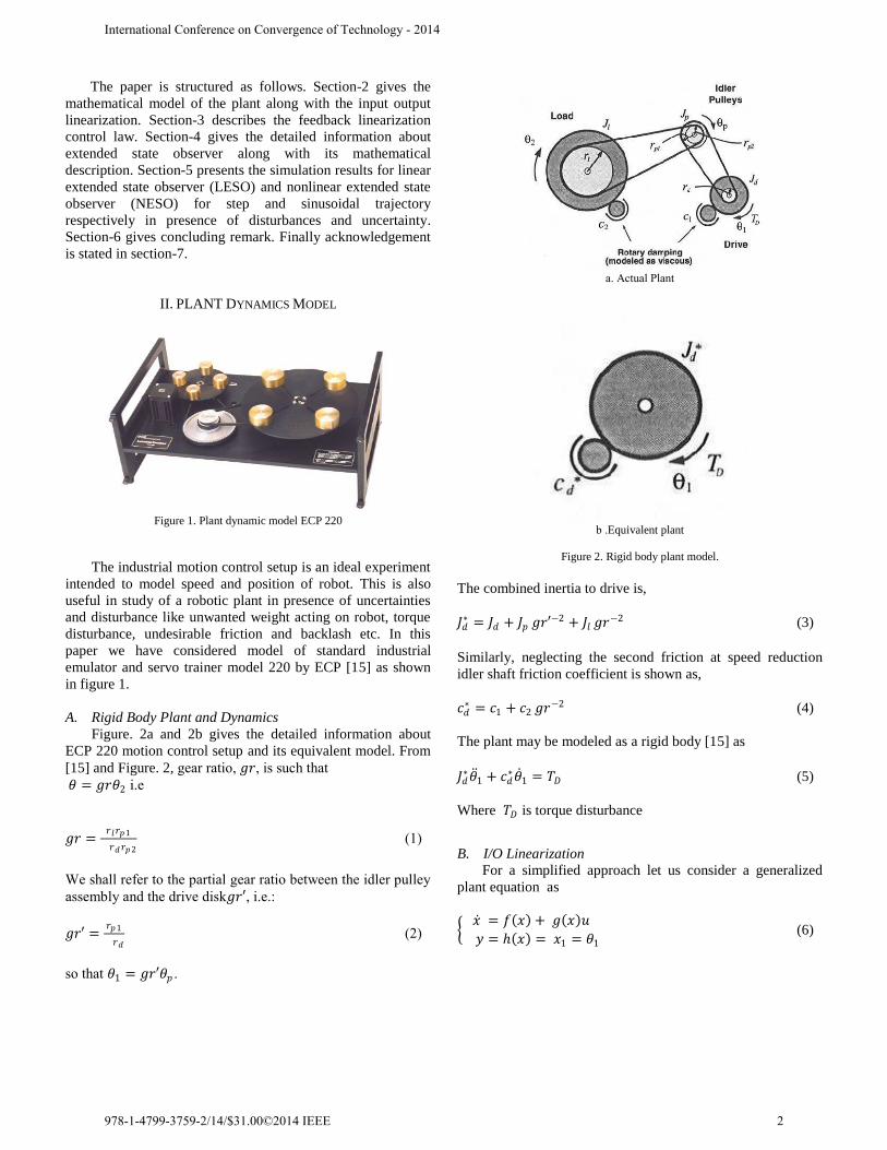
Figure 1. Plant dynamic model ECP 220

The industrial motion control setup is an ideal experiment

intended to model speed and position of robot. This is also

useful in study of a robotic plant in presence of uncertainties

and disturbance like unwanted weight acting on robot, torque

disturbance, undesirable friction and backlash etc. In this

paper we have considered model of standard industrial

emulator and servo trainer model 220 by ECP [15] as shown

in figure 1.

A. Rigid Body Plant and Dynamics

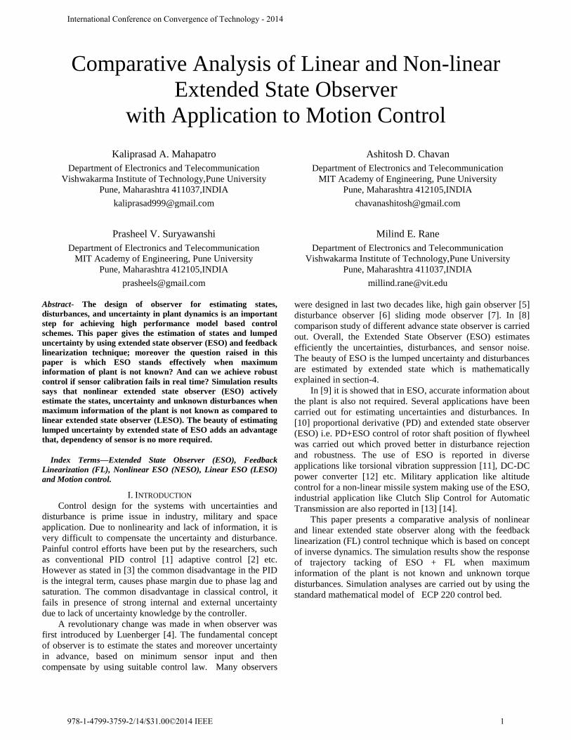
Figure. 2a and 2b gives the detailed information about

ECP 220 motion control setup and its equivalent model. From

[15] and Figure. 2, gear ratio, 𝑔𝑟, is such that

𝜃 = 𝑔𝑟𝜃2 i.e

𝑔𝑟 =𝑟𝑙𝑟𝑝1

𝑟𝑑𝑟𝑝2 (1)

We shall refer to the partial gear ratio between the idler pulley

assembly and the drive disk𝑔𝑟′, i.e.:

𝑔𝑟′ =𝑟𝑝1

𝑟𝑑 (2)

so that 𝜃1 = 𝑔𝑟′𝜃𝑝 .

a. Actual Plant

b .Equivalent plant

Figure 2. Rigid body plant model.

The combined inertia to drive is,

𝐽𝑑∗ = 𝐽𝑑 + 𝐽𝑝 𝑔𝑟′

−2 + 𝐽𝑙 𝑔𝑟−2 (3)

Similarly, neglecting the second friction at speed reduction

idler shaft friction coefficient is shown as,

𝑐𝑑∗ = 𝑐1 + 𝑐2 𝑔𝑟

−2 (4)

The plant may be modeled as a rigid body [15] as

𝐽𝑑∗𝜃 1 + 𝑐𝑑

∗𝜃 1 = 𝑇𝐷 (5)

Where 𝑇𝐷 is torque disturbance

B. I/O Linearization

For a simplified approach let us consider a generalized

plant equation as

𝑥 = 𝑓 𝑥 + 𝑔 𝑥 𝑢

𝑦 = 𝑕 𝑥 = 𝑥1 = 𝜃1

(6)

International Conference on Convergence of Technology - 2014

978-1-4799-3759-2/14/$31.00©2014 IEEE 2

As stated in [16], trajectory tracking can be designed by using

geometric control theory based on feedback linearization.

Considering space coordination 𝑧𝑖 . Let

z = ∅1(𝑥)

∅2(𝑥) =

𝐿𝑓0 (𝑥)

𝐿𝑓1 (𝑥)

(7)

Where 𝐿𝑓 h is called lie derivative of h w.r.t . 𝑓. As defined in

[16], h:ℜ𝑛 → ℜ be a smooth scalar function and 𝑓 : ℜ𝑛 →

ℜ𝑛 be a smooth vector field ℜ𝑛 then the lie derivative of h

w.r.t . 𝑓 is a scalar function defined by

𝐿𝑓 𝑕 = ∇𝑕𝑓 (8)

Therefore from above stated concept and [15][17] and

equation (5). The dynamics in new coordinate model can be

written as

𝑧 1𝑧 2 =

𝑧2

−𝑐𝑑∗

𝐽𝑑∗ 𝑧2 +

𝑇𝐷

𝐽𝑑∗ +

01

𝐽𝑑∗ u (9)

Where u = control voltage.

III. FEEDBACK LINEARIZATION

A single input non-linear system in the form of equation

(6) with f(x) and g(x) being smooth vector fields on ℜ𝑛 is said

to be input- state linearizable if there exist a region Ω in ℜ𝑛

adiffeomorphism Φ = Ω → ℜ𝑛 and a non linear feedback

control law

𝜐 = 𝛼 + 𝛽𝑢 (10)

Where u is the control voltage 𝑉𝑚 such that 𝑧 = 𝜙(𝑥) and

the new input 𝜐 satisfy a linear time invariant relation,

𝑧 = 𝐴𝑧 + 𝐵𝑢 (11)

From equation (10) define a new 𝜐 in the linearized system,

then the relationship between u and 𝜐 becomes

𝑢 =𝜐−𝛼

𝛽 (12)

Then non-singular system is linearzed as

𝑧 = 0 10 0

𝑧 + 01 𝜐 (13)

𝑦 = 1 0 𝑧 (14)

The system is linear and controllable, and it can be stabilized

by state feedback or optimal control.

Now taking new input 𝜗 as

𝜗 = 𝜗𝑐 + 𝑘1(𝜗𝑐 - 𝑧1) + 𝑘2(𝜗 𝑐 - 𝑧2) (15)

where the 𝜗𝑐 represent the reference trajectory. Applying the

control law to (11), the tracking error dynamics can be written

as

d2e

dt 2 + 𝑘2𝑑𝑒

𝑑𝑡+ 𝑘1𝑒 (16)

Where 𝑒 = (𝜗𝑐 − 𝑧1)is the tracking error. The gain values

of 𝑘𝑖 are chosen appropriately to achieve desired trajectory

tracking of reference signal 𝜗𝑐 . From (15) and (12) the control

input u can be rewritten as

𝑢 = 1

𝛽[𝜗𝑐 + 𝑘1 𝜗𝑐 − 𝑧1 + 𝑘2 𝜗 𝑐 − 𝑧2 − α] (17)

However as shown in equation (17), it is very difficult

practically to guarantee the exactness of 𝛽 and 𝛼 due to

uncertainty and disturbances.

Let us assume that we know some information about the plant.

Let 𝛽 = 𝑏0 and 𝛼 = 𝑎0 + 𝑑 where d = associated lumped

uncertainty and disturbance

𝑢 = 1

𝑏0[𝜗𝑐 + 𝑘1 𝜗𝑐 − 𝑧1 + 𝑘2 𝜗 𝑐 − 𝑧2 − 𝑎0 − 𝑑] (18)

IV. EXTENDED STATE OBSERVER

In order to design a controller which will work when

some information about the plant i.e. 𝑎0 𝑏0 , in presence of

lumped uncertainty and disturbances d and to find exact

information about the states 𝑧𝑖 of the plant without maximum

dependencies on practical plant (i.e. without maximum

sensors) it is very essential to estimate the state 𝑧𝑖 and

perturbed systems d. In this paper we have estimated by using

an Extended State Observer (ESO). Extended state observers

offer a unique theoretical fascination. The concept is based on

linear as well as non-linear systems, dynamic response,

controllability, observability and stability, and provides a

relation [18] in which all of these concepts interact. ESO

estimates states of the plant along with uncertainty and

disturbances of plant and sensors. Moreover it is independent

of plant model. Overall it performs better than other observer

and it is very simple to implement practically.

A. Mathematical Interpretation of ESO

In general, the nth

order non-linear equation is represented

as,

𝑧 𝑛

= 𝑓 𝑧, 𝑧 ,…… . 𝑧 𝑛−1

,𝜔 + 𝑏𝑢 (19)

Where 𝑓 . represent the dynamics of the plant + disturbance.

𝜔 is the unknown disturbance (𝑇𝐷 ) in our case. u is the

control effort given in voltage. z is the measured output.

𝑏 = 𝑏0 + Δ𝑏 where 𝑏0 is the best known value. The Equation

(19) is augmented as

International Conference on Convergence of Technology - 2014

978-1-4799-3759-2/14/$31.00©2014 IEEE 3

𝑧 1 = 𝑧2 𝑧 1 = 𝑧3

. (20)

. 𝑧 𝑛 = 𝑧𝑛+1 + 𝑏0𝑢

𝑧 𝑛+1 = 𝑕 𝑦 = 𝑧1

In state-space notation

𝑧 = 𝐴𝑧 + 𝐵𝑢 + 𝐸𝑕 (21)

Here 𝑓(𝑧, 𝑧 ,𝜔) and its derivative 𝑕 = 𝑓(𝑧, 𝑧 ,𝜔) are assumed

to be unknown, by using state estimator it is now possible to

estimate 𝑓(𝑧, 𝑧 ,𝜔) for (20). A non-linear observer was

proposed in [3] as

𝑧 1 = 𝑧 2 + 𝛽1𝑔1 𝑒 ⋮

𝑧 𝑛 = 𝑧 𝑛+1 + 𝛽𝑛𝑔𝑛 𝑒 + 𝑏0𝑢

𝑧 𝑛+1 = 𝛽𝑛+1𝑔𝑛+1 𝑒

(22)

Where 𝑒 = 𝑦 − 𝑧 1 is the error, 𝑔𝑖 . is a nonlinear gain

satisfying 𝑒 × 𝑔𝑖 > 0 ∀ 𝑒 ≠ 0. If one chooses the nonlinear

function 𝑔𝑖 . and their related parameters properly, the

estimated state variable 𝑧 𝑖 are expected to converge to the

respective state of the system 𝑧𝑖 , i.e. 𝑧 𝑖 → 𝑧𝑖 The choice of 𝑔𝑖 is heuristically given in [8]

𝑔𝑖 𝑒,𝛼𝑖 , 𝛿 = 𝑒 𝛼𝑖 , 𝑒 > 𝛿

𝛿𝑒

1−𝛼𝑖 , 𝑒 ≤ 𝛿 (23)

Where 𝛿 is the small number (𝛿> 0) which add limit to the

gain, 𝛽 is the observer gain carried by the pole-placement

method.𝛼 is normally selected between 0 and 1 for Non-linear

ESO (NESO) and is considered unity in Linear ESO (LESO)

In (22), 𝑧 1, 𝑧 2 … . 𝑧 𝑛 estimate the state of plant and 𝑧 𝑛+1 is the

extended state which estimates the uncertainties in plant,

which adds robustness in our controller design. The LESO for

the system is designed by making 𝛼 = 1 i.e. gain g(e)=e . The

state-space model, can be written as

𝑧 = 𝐴𝑧 + 𝐵𝑢 + 𝐿𝐶(𝑧 − 𝑧 ) (24)

Where

L = [𝛽1𝛽2…… 𝛽𝑛𝛽𝑛+1] T

(25)

is the observer gain vector

B. Robust Control

Integrating the discussion carried out in section 3 and 4

respectively the robust control of motion plant can be designed

as shown in figure 3.

According to our plant extended state observer along with

feedback linearization control can be designed as

𝑧 1 = 𝑧 2 + 𝛽1𝑔1(𝑒)

𝑧 2 = 𝑧 3 + 𝛽2𝑔2 𝑒 + 𝑏0𝑢

𝑧 3 = 𝛽3𝑔3 𝑒 𝑦 = 𝑧1

(26)

Now instead of using practical state 𝑧1 and 𝑧2 in equation

(18) we will use estimated state 𝑧 1 and 𝑧 2 and lumped

uncertainty and disturbance will be estimated by extended

state 𝑧 3. Therefore control effort 𝑢 will take the form

𝑢 = 1

𝑏0[𝜗𝑐 + 𝑘1 𝜗𝑐 − 𝑧 1 + 𝑘2 𝜗 𝑐 − 𝑧 2 − 𝑎0 − 𝑧 3] (27)

V. SIMULATION RESULTS

By considering the nominal values of the plant from [15]

equation (9) can be rewritten as.

𝑧 1𝑧 2 =

𝑧2

−1.41𝑧2 + 23.2𝑇𝐷 +

023.2

𝑢 (28)

From equation note that 𝑏0 = 23.2 actually but to make the

system more realistic we have consider 𝑏0 = 38 i.e. ∆𝑏 𝑢 =(23.2 − 38)𝑢 is the associated uncertainty in the plant.

Torque disturbance 𝑇𝐷 is considered as 1𝑉 𝑎𝑛𝑑 1 × sin(𝑡)

step and sinusoidal voltage which corresponds to 10% of

maximum torque when step of 1𝑉 and sinusoidal voltage of

6𝑉 are applied respectively. Therefore practical plant can be

written as

𝑧 1 = 𝑧2

𝑧 2 = −1.41𝑧2 + 23.2𝑇𝐷 + 23 − 38 𝑢 + 38𝑢

= 𝑓 + 38𝑢 (29)

The controller gains are taken as 𝑘1 = 16 𝑎𝑛𝑑 𝑘2 = 8. Observer gain as 𝛽1 = 26.6 ,𝛽2 = 169.11 𝑎𝑛𝑑 𝛽3 = 315.13 calculated via pole placement method. The results divided in

two sections as Linear Extended State Observer (LESO) and

Nonlinear Extended State Observer (NESO)

International Conference on Convergence of Technology - 2014

978-1-4799-3759-2/14/$31.00©2014 IEEE 4

Figure 3. ESO and FL block for estimating states, uncertainty and disturbances

A. LESO

LESO is designed by considering 𝛼 = [1 1 1].

a. Step Position Tracking

b. Step Velocity Tracking

Figure 4. (-) States and (--) Estimated States for step trajectory

a. Position Tracking for sinewave

b. Velocity Tracking for sinewave

Figure 5. (-) States and (--) Estimated States for sine trajectory

B. NESO

NESO is designed by considering 𝛼 = [1 0.5 0.25].

a. Step Position Tracking

International Conference on Convergence of Technology - 2014

978-1-4799-3759-2/14/$31.00©2014 IEEE 5

b. Step Velocity Tracking

Figure 6. (-) States and (--) Estimated States for step trajectory

a. Position Tracking for sinewave

b. Velocity Tracking for sinewave

Figure 7 (-) States and (--) Estimated States for sine trajectory

VI. CONCLUSION

1. In this paper a robust control algorithm for an

industrial motion control setup is proposed by

integrating feedback linearization with extended state

observer.

2. From figure 4, 5 and figure 6, 7 it is clear that, for

different trajectory, nonlinear extended state observer

(NESO) provides superior estimation of states,

uncertainty and disturbances.

3. By choosing 𝛼 as 0 < 𝛼 ≤ 1 the transient error can

be significantly reduced.

4. Minimum converging time i.e. speeds and accuracy

of states of observer converges to those of plant in

NESO.

5. From the simulation result and figure 3 following

conclusion can be drawn

If we assumed calibration error in position

sensor by adjusting proper observer gains

better estimation of position can be done.

Moreover, by having information of

position sensor alone the ESO is able to

estimate velocity. Therefore dependency of

sensor is reduced.

VII. ACKNOWLEDGEMENT

The principal author is thankful to MIT Academy of

Engineering, Alandi (D), Pune (Instrumentation and Control

Lab) for the use of advance lab equipments and software for

carrying out this work.

REFERENCES

[1] K. J. Astrom and T. Hagglund, PID controllers: Theory, design

and tuning. Research Triangle Park, N.C. “Instrument Society of

America”, 1995.

[2] K. J. Astrom and B. Wittenmark, Adaptive Control, 2nd edition,

Reading MA: Addison-Wesley, 1995.

[3] Jingquin Han. From PID to active disturbance rejection control.

“IEEE Transactions On Industrial Electronics”, 56(3):900 – 906,

March 2009.

[4] David G. Luenberger, An Introduction to Observer “IEEE

Transaction on automatic control”, vol. 16, no. 06, pp. 596 -

602, Decembers 1971.

[5] Khalil. H. K. High-gain observers in nonlinear feedback control.

“New Directions in Nonlinear Observer Design” Vol. 24(4).

1999. pp: 249

268.

[6] J. J. E. Slotine, J. K. Hednck, and E. A. Misawa, “On sliding

observers for nonlinear system” Journal of Dynamic Systems,

Measurement, and Control” Vol. 109, 1987, pp 245-252.

[7] A. Radke and Z. Gao, A survey of state and disturbance

observers for practitioners, "American Control Conference”, pp.

5183 - 5188, June 2006.

[8] Weiwen Wang and Zhiqiang Gao. A comparison study of

advanced state observer design techniques. “In Proceeding of

the American Control Conference”, pages 4754 – 4759, Denver,

Colorado, 2003.

[9] Z. G. Qing Zheng, Linda Q. Gao, On validation of extended

state Observer through analysis and experimentation, ”Journal of

Dynamic Systems, Measurement, and Control, ASME”, vol.134,

2012.

[10] B. X. S. Alexander, Richard Rarick, and Lili Dong. A novel

application of an extended state observer for high performance

control of NASA’s HSS flywheel and fault detection.

“American Control Conference”, pages 5216 – 5221, June 2008.

[11] Ruicheng Zhang, Zhikun Chen, Youliang Yang, and Chaonan

Tong.. Torsional Vibration Suppression Control in the Main

drive system of Rolling Mill by State Feedback speed Controller

Based on Extended State Observer, “IEEE international

conference on control and automation” pages 2172 – 2177,

Guangzhou, CHINA, May 2007.

[12] B. Sun and Z. Gao. A DSP based active disturbance rejection

control design for a 1-kwh bridge dc-dc power converter.

“IEEE Transactions on Industrial Electronics”, 52(5):1271 –

1277, October 2005.

[13] Y. Xia, Z. Zhu, and M. Fu. Back-stepping sliding mode control

for missile systems based on an extended state observer. “IET

Control Theory and Applications”, 05:93 – 102, March 2011.

[14] Yunfeng Hu, Qifang Liu, Bingzhao Gao, and Hong Chen.

“ADRC Based Clutch Slip Control for Automatic Transmission”

IEEE Chinese Control and Decision Conference (CCDC)., pages

2725 – 2730, 2011.

[15] ECP, Model 220 Industrial Plant Emulator, Educational Control

Products, Canada.

International Conference on Convergence of Technology - 2014

978-1-4799-3759-2/14/$31.00©2014 IEEE 6

[16] Jean Jacques E. Slotine and Weiping Li. “Applied Nonlinear

Control”. Prentice Hall, New Jersey, U.S.A, 1st edition, 1991.

ISBN 0-13-0408905.

[17] Z. Gao, Scaling and bandwidth-parameterization based

controller tuning, “American Control Conference”, pp. 4989-

4996, June 2003.

[18] Aaron Radke and Zhiqiang Gao. A survey of state and

disturbance observers for practitioners. “In Proceedings of the

2006 American Control Conference”, pages 5183 –5188,

Minnesota, USA, June 2006.

International Conference on Convergence of Technology - 2014

978-1-4799-3759-2/14/$31.00©2014 IEEE 7