-R179 445 A NEW PUNPJET DESIGN TI4EORY(U) TETRA TECH INC PASADENA i.'1CA 0 FURUYA ET AL 25 FEB 87 TETRAT-TC-1037-01M80614-85-C-8856

UNCLASSIFIED F/6 1211 M

Ehmhhhhhhhilmhhhhhhhhhhhml0

%

Nq

. . . -

12.

1.25 1- 1325 W1._-..___

.. h.,.

MICROCOPY RLSOLUIICN TISI CHARI

% %-. %J

-.. 3.

V--.I,'

U. e . - ' ..... 3_ .

. . . . . .. . . V' " " "; ' * "" V"' . .. " ', *,',"." ",',

* n

Report No. TC .3037-01

~iF ILEnu Cir~OPYVii

A NEW PUMPJET DESIGN THEORY

by

OKITSUGU FURUYA m'WEN-LI CHIANG

TETRA TECH, INC.630 NORTH ROSEMEAD BOULEVARD

*PASADENA, CALIFORNIA 91107

* FEBRUARY 198/ CTIC~m~

Prepared for

DAVID W. TAYLOR NAVAL SHIPRESEARCH AND DEVELOPMENT CENTER

BETHESDA, MARYLAND 20084

OFFICE OF NAVA. RESEARCH-a 800 NORTH QUINCY STREET

ARLINGTON, VIRGINIA 22217-5000

Approved for public release;distribution unlimited

R7 4 '

Report No. TC-3037-01Contract No. N00014-85-C-0050

*

A NEW PUMPJET DESIGN THEORY

by

OKITSUGU FURUYA

WEN-LI CHIANG

TETRA TECH, INC.

630 NORTH ROSEMEAD BOULEVARDPASADENA, CALIFORNIA 91107

* FEBRUARY 1987

Prepared for

U ,' DAVID W. TAYLOR NAVAL SHIPRESEARCH AND DEVELOPMENT CENTER - ,.

BETHESDA, MARYLAND 20084 ,

= '. APR 2 1 !987 N

OFFICE OF NAVAL RESEARCH A 2 7 !800 NORTH QUINCY STREET .ARLINGTON, VIRGINIA 22217-5000

oAApproved for public release;distribution unlimited

-.

SUCUOIIT~ CL.ASSIFICATION4 OF TWIS JDAGE (10hen O.ts Znteedl

REPORT DOCLUME14TATICN PAGE 1 VOECMLE"N O-1. A&PORT 414141191 1Z. GOVT ACCWSION 04O 1. iRZCIPENT*S CAAL.00 NUMOCR

* TC-3037-011*4. ?I11 (end Suatiitle) S. 09_O R9PON? -S PRRIOO COVIREO

*Technical - Theory & Experimer

A NEW PUMPJET DESIGN THEORY Jan. 1, 1986 - Dec. 31, 1986

____ ___ ____ ___ ____ ___ ___ ____ ___ ____ ___ ___TC-3037-01

7. AUhR~ .cohntACT- R GAA~t SUMdCl(*I

0. Furuya Ia.W.-L. Chiang N00014-8 5-C-OO 50

I . RORMING ORGANIZA?IC 4 A149 AMC AOORIESS 1-3. PROGAAM ElLUEN7.12CJEC. rASK

* ~Tetra Tech, Inc. AE R N1 U8R

* 630 N. Rosemead Blvd.Pasadena, CA 91107

5 i. cOM~otr L:soOO9ICgbAhig A4O AOORISS 12. AREPORT OAT9*DWTNSRDC February 25, 1987

Dept. of the Navy 1*3. NUMJR CIFPASBethesda, MD 20084 52

Ill. O4IOR#..0 A43INCY MAME & AOORES9S(If diffeent fro Caiu.1Zlini Ollie*) IS5. SECUAIt'Y CL.ASS. (.1 fhi. eFP0e0f)

Office of Naval Research Ucasfe800 North Quincy St.Arlington, VA 22217-5000 s.oc.As'CrN/OWGOt4

14. OI3?RtISUU OM STATEMENT (*I as i Re.,

Approved for public release; distribution unlimited ..

17. 2j~~§~O 3TATZMIEN? (at the &&*tract entered In Slack 20. It differmnt Imen Repel?) p

a14. $UPPR.V*MNARY P44Q'PS

Sponsored by the Naval Sea Systems Command General Hydrodynamic ResearchProgram and administered by the David W. Taylor Naval Ship R&D Center,Code 1505, Bethesda, MD 20084.

It. KEY VOACS :Candinue 1"4 ?0-009G 14I ?dW di*I 0 047 and afttl 7 4y bide& flhii r)

Pumpjet-Streamline Curvature Method e

Blade-to-Blade MethodFlow Skewness

40. ASTRACT7 (G4nhflftd in w. old* U.IRece6*4r mid doaftty ar bloca ?iiNZ'a)

The pumpiet is a unique fluid machine whichltrti1fe retarded wake flow and6L produces high propulsive efficiency such as 90%. The existing pumpjet design

method is based on a simple two-dimensional graphic method which was used forpump design. As the demand for the speed of underwater vehicles, increased in

- recent years, the existing design method became inappropriate. Effort has beenmade to develop a new three-dimensional pump design method by combining a blade-

through flow theory with blade-to-blade flow theory. Such a method requires

0 14 73 eoirvapi OF91 mov 1313oasOLigtl U N C L AS S I F I E D

.................................. A. T. MZ F. .'l .. .. .- . . . .. -

"L.umW? cu.AsSAViCATIW ?io i ns PAOetho Does got~~

20. many supporting sub-theories to be developed. The foundation work for theblade-through flow theory, i.e., streamline curvature method, three-dimensional flow mapping technique, as well as two-dimensional cascadetheory, has -bee established in the FY-85 GHRtprogram. During this FY-86GHR program, the blade-to-blade flow theory with corrections due to thethree-dimensionality has been established. Particularly, the flow skewnesswhich escaped many researchers has been found essential for accurate design

a-. of pumpjet.

7'

16M

4,%

U N CL A SS I FI E

19U NCLASSIFI EDINO 43 A917MDaaetr*

01;R! LSIIAIO PI agfl'l O.Z~e.

TABLE OF CONTENTS

Page WY

L IST OF FIGURES.............................*i

1.0 BACKGROUND...................................I

2.0 OBJECTIVES.................................... 4

3.0 THREE-DIMENSIONAL DESIGN METHOD ..................... 53.1 BLADE-THROUGH FLOW ANALYSIS - STREAMLINE

*CURVATURE METHOD ........................ 73.2 TWO-DIMENSIONAL ANALYSIS ................. 7 'W

3.2.1 Linearized Cascade Theory...............73.2.2 Data Analysis........ ........... 11

3.3 THREE-DIMENSIONAL ANALYSIS - BLADE-TO-BLADEF LOW .................................. 12

40 3.3.1 Differential Equations.............. 123.3.2 Transformation ........ ......... .... 133.3.3 Effects of Streamline Inclination and

Meridian Velocity Variation........... 143.3.4 Induced Velocities .............. 163.3.5 Boundary Condition ...................... 19

*3.3.6 Flow Skewness in Diagonal ContractingChannel ........................ 20

3.3.7 Secondary Flow Correction........... 263.4 DESIGN PROCEDURE......................... 26

4.0 CONCLUSIONS .......... . .. ... ................. .. 29

5.0 REFERENCES ........ ........................... 30

%Aw

App.'

LIST OF FIGURES, .. 1-*_

- Figure Page

1-1 A typical pumpjet blade and shroud con-figuration 32

AP 1-2 A typical meridional flow velocity (Vm)distribution for a pumpjet where V® is theupstream flow velocity 32

1-3 A typical load distribution in terms ofVe for pumpjet rotor blade where V9 is the

0 circumferential component of the turned F-flow velocity 33

1-4 Typical pumpjet rotor blade configuration,(a) top view and (b) upstream view 34

4 3-1 Flow chart of the selected pumpjet design

method 35

3-2 Definition diagram 36

3-3 Variation of design angle of attack withsolidity for the sections tested 37

3-4 Comparison of design angle of attack obtainedfrom the multiple regression analysesand those obtained from the laboratory 38

3-5 Camber as a function of cascade lift coef-ficient and solidity obtained from regression %-.4

analysis data (solid line) compared withoriginal data (discrete data point), for

81 = 30'3

3-6 Camber as a function of cascade lift coef- I!ficient and solidity obtained from regressionanalysis data (solid line) compared with

*, original data (discrete data point), for81 = 4 40

3-7 Camber as a function of cascade lift coef-ficient and solidity obtained from regressionanalysis data (solid line) compared withoriginal data (discrete data point), for

81=60* 41

in "'*"ii

i i .,.',,- "-- -

List of Figures (Continued)

Figure Page

3-8 Camber as a function of cascade lift coef-ficient and solidity obtained from regressionanalysis data (solid line) compared withoriginal data (discrete data point), forBi = 70" 42 -.

3-9 Axisymmetric stream surface 43

3-10 Blade setting in the mapped plane 44

3-11 Flow configuration in contraction channel 45 ,-

3-12 Flow skewness on the velocity diagram due tovortex distribution 46

3-13 General flow chart to design blade ina flow of three-dimensional character 47

3-14 Flow chart for Subroutine INP 48

3-15 Flow chart for Subroutine INP2 49

3-16 Flow chart for Subroutine MAP32 50

3-17 Flow chart for Subroutine DSN2 51

3-18 Flow chart for Subroutine PFM3 52

4P

' ,°°% Si

i ii .'"'"1• .,

" 1.0 BACKGROUND

The pumpjet is considered to be one of the most promising

candidate propulsors for high speed underwater vehicles and,

as a matter of fact, it has recently been employed for MK-48

torpedoes, ALWT--Advanced Light Weight Torpedo (now called

MK-50), and other underwater vehicles. The pumpjet

superiority over other propulsion devices is represented by

two major factors, i.e., high efficiency and quietness.

The pumpjet is one of few fluid devices which positively

-I utilizes retarded wake flow and produces high propulsive

efficiency. This peculiar situation may be understood

readily by considering the momentum equatn applied to a

control volume surrounding an underwater vehicle, fixed to0the inertial coordinate system. For a conventional pro-

peller, the velocity of flow coming into a propeller blade

is approximately equal to the vehicle speed since the pro-

peller diameter is large enough to enjoy the free stream

flow. In order for the propeller to generate an effective

thrust, it should accelerate the flow, the ejected flow

speed being faster than the incoming flow. It means that a

certain amount of the energy imparted on the fluid by the

-. thruster is dumped in the surrounding water. On the other

hand, for a pumpjet, the incoming flow velocity is retarded

and slower than the free stream velocity. In order to

generate a thrust, again this flow has to be accelerated.

However, if the pumpjet is properly designed, the acceler-

ated flow velocity can be almost the same as the vehicle

speed. The ejected flow out of the pumpjet has little rela-

tive velocity and thus leaves hardly any jet wake behind the

vehicle. Compared to a vessel with a conventional pro-

peller, a vehicle with a pumpjet generates much less wasted --.

energy in the flow field. This is the major reason why the

pumpjet can produce a high propulsive efficiency such as 90%

P or higher when it is properly designed. TI

Ar1

.1-. -.). " , • .1

6'"- __

Quietness is a guaranteed aspect with the pumpjet. As can

be seen from its configuration (Figure 1-1), a long shroud

completely surrounding the rotor helps prevent rotor noise

from emitting into the outside flow field. Furthermore,

this "internal" flow machine has better resistance charac-

* teristics against cavitation, resulting in quieter shallow

water operation where propulsors are most susceptible to

cavitation.

However, in order to achieve such a high standard of perfor-

mance, there are many penalties to be paid in reality. The

first such penalty naturally stems from the pumpjet's util- It.

izing the velocity-retarded wake flow. A typical meridional

flow distribution at the inlet of pumpjet rotor is shown in

Figure 1-2; the velocity at the hub is only 30% of the free

stream velocity and rapidly increases to 75% at the shroud ...

internal boundary. This large velocity gradient in the

transverse direction is, of course, built up by the viscous

boundary layer effect and is one of the key features causing

difficulties in design, fabrication and eventually in

achieving the pumpjet high performance.

When one designs an axial or a near axial pump, it is cus-

tomary to distribute the blade loading from hub to tip in a

forced vortex or a free vortex distribution method, such as

shown in Figure 1-3. Such distribution methods are impor-

tant in obtaining a nearly uniform discharge jet behind the

rotor in order to minimize the mixing loss. However, a

serious problem arises in attempting to implement either

forced vortex or free vortex loading distribution against

the flow field having a large velocity gradient as shown

in Figure 1-2. Due to the lack of enough meridional flow

velocity near the hub, the blade there should be designed

to have extremely large incidence angle as well as large

camber. It is for this reason that the pumpjet rotor

designed to date has a distorted profile shape from hub to

tip (Figure 1-4). If this were a conventional propeller,

2... . . . . . . .. . . . .,- '*- -*.*.*, . - - * * * * * * * . . .-. .. , ,

U

* the stagger angle would become smaller towards the hub and

the camber would stay more or less constant. However, for

the reason mentioned above, the pumpjet blade stagger angle

first becomes smaller up to the midspan area but becomes

larger toward the hub and thus the camber is designed to be

substantially larger.

This unusual rotor blade setup causes various hydrodynamic

problems. Since a typical flow incidence angle near the hub

* has to be extremely high (e.g., 30"), even a slight error in

design may cause flow separation, possibly cavitation and

then noise generation. Furthermore, even if design is made

properly, the same vulnerable situation is generated with a

slight flow disturbance or blade deformation due to fabrica-

tion inaccuracy1 . The existing one-dimensional graphic

pumpjet design method with empirical corrections for the

cascade effect fails to design a pumpjet free of flow

separation. The three-dimensional effect due to the diag-

onal flow configuration and the cascade effect are not prop-

erly taken into account. It is for this reason that

development of a more accurate three-dimensional pumpjet

design theory is in order.

* I Some pumpjet rotors are produced by investment castingprocess so that the fabrication accuracy cannot be

expected to be high.

3

2.0 OBJECTIVES

The objectives of the work under the GHR program are:

1) to develop a more reliable and accurate pumpjetdesign theory based on a three-dimensional pump jdesign concept, .T,

t 2) to accurately incorporate the cascade effect intothe theory and then,

3) to improve the pumpjet performance characteristics. jThe objective of the FY-86 study was to develop a mathemati-

cal model for the blade-to-blade flow for the three-

dimensional pumpjet design method selected in FY-85. In

FY-86, the blade-through flow theory will be incorporated 2into the blade-to-blade theory, resulting in forming a

complete three-dimensional pumpjet design theory.

411 •: -w ...

4

**.•;W ..

3.0 THREE-DIMENSIONAL DESIGN METHOD

Design of a pumpjet for an underwater vehicle requires pre-

liminary information on the vehicle including its geometry

and hydrodynamic drag coefficient. Furthermore, most

importantly, the velocity profile at an upstream reference

section should be obtained either analytically or

experimentally. Any error in the velocity profile would

result in a pumpjet of lower efficiency or failure of the

pumpjet meeting the specifications at the design point. In

the present study, it is assumed that this velocity profile

is given at a goal speed or at the corresponding Reynolds

number.

The first step for design of a pumpjet (Figure 3-1) is todetermine the shroud intake diameter. From the viewpoint

of cavitation, the maximum and minimum shroud diameter to

prevent cavitation must exist. If it is too large, the

rotor blade tip speed becomes too high so that cavitation

occurs. On the other hand, if it is too small, the rotation

speed must be increased to generate the required head so

that the chance of cavitation inception also increases.

Another aspect of determining the shroud diameter stems from

the consideration of overall propulsive efficiency. The

equation for global momentum balance should be able to

determine an efficiency-optimum shroud diameter for the

given velocity profile and vehicle drag.

Once the shroud diameter is determined, streamlines will

be calculated by using the streamline curvature method

(SCM). In this calculation, the loading distribution on the

rotor and blade thickness must be assumed in advance. One

of the major concerns in using the existing streamline cur-

vature method lies in the fact that SCM may only be used for

relatively uniform incoming flow, but may generate a sub-

stantial error for a thick wake flow, i.e., highly retarded

flow due to the viscous boundary layer on the vehicle hull.

*~~ 5

-3-A en

Detailed mathematical formulation and sample calculations

-" have been presented in the 1985 report (Furuya and Chiang,

4p 1986). Also included are discussions regarding the problems

of application of conventional SCM to the thick wake flow.

5'. The next step of the design method is to map the stream tube

or surface calculated by SCM onto a plane so that the rotor

blades are mapped into cascade configuration. If the stream

surface is totally cylindrical shape, the governing equation

to be used for the cascade analysis will be a Laplace - -

equation. Unfortunately, the stream surface is of three-dimensional cone shape in general for the tail cone section

of the underwater vehicle. The field governing equation now

becomes a Poisson equation, and the results of powerful

potential theory analysis are no more applicable. A method

of correcting the effect of the Poisson equation on the

potential theory results is introduced to modify the blade

profile shape obtained in the potential theory. In choosing

the blade profile shape, the experimental data are used to

ensure that there is no chance of flow separation due to

overloading on the blade. Furthermore, based on the calcu-

lated velocity along the blade, the cavitation inception is

checked. If there exists a chance of either flow separation

or cavitation, the loading distribution from hub to tip

should be changed. If such a change is made, and/or

thickness of blades is changed, the streamline curvature

method should be used again to determine the new location of

streamline or stream surface. This iterative procedure is

: to be repeated until an overall convergent solution is

obtained. Section 3.3 describes the technical approach to

be used for the blade-to-blade flow analysis. The two-

dimensional theory applicable to the mapped stream surface

is summarized in Section 3.2. The overall product of three-

dimensional pumpjet design is described in Section 3.4.

U'

6

~C%2

- - - -

3.1 BLADE-THROUGH FLOW ANALYSIS - STREAMLINE CURVATUREMETHOD

The mathematical formulation for the streamline curvature

method (SCM) has been described in the 1985 report (Furuya

and Chiang, 1986).

3.2 TWO-DIMENSIONAL ANALYSIS

In the following, the major concept of Mellor's two-

dimensional cascade theory will be summarized for the

reader's convenience.

3.2.1 Linearized Cascade Theory

A two-dimensional cascade theory is implemented here to be

used for calculating the lift coefficient for the three-

dimensional flow discussed in Section 3.3. The boundary

conditon (Eqn. 3.2-14) has to be modified, as discussed in

Section 3.3, when this cascade theory is applied in the

q quasi three-dimensional flow.

The lift coefficient is determined for any given cascade

geometry which is specified by the solidity (blade chord-gap

ratio, c/s) and the stagger angle, X (Figure 3-2). Symbols

used in Mellor (1959) were followed; use Li and CLi in

denoting the ideal lift force and lift coefficient when the

drag is zero. Then (see also Weinig, 1964)

Li = (s/c)PWmAVe (3.2-1)

and CLi : (Li/c)/(2pWm2)

- 2(s/c)(AVe/Wm) (3.2-2)

where s is the blade pitch, c is the chord length, p is the

fluid density, Wm is the mean relative velocity, and AVe is

the difference between the peripheral velocity at the exit

and that at the inlet.

7

-1-,

Vb.

Replacing the product sAVe by the line integral pv-dr on a

closed path comprising two streamlines s distance apart and

Pr. joined by two lines parallel to the e-direction, we have

(Weinig, 1964)

, CLi : 2r/(CWm) (3.2-3)

* where r *7dr (3.2-4) p-.

is the circulation around a profile (Wislicenus, 1965).

The camber is assumed to be sufficiently small so that the*chord length is substantially equal to the distance measured

along the camber line. Then, the circulation around a thin

wing profile is given by (Abbott and von Doenhoff, 1959)

wr = eo y dx (3.2-5)

where y is the difference in velocity between the suction

and pressure surfaces, which is also the strength of the

vortex sheet comprising the blade camber line (von KdrmIn

and Burgers, 1963). Therefore, equation (3.2-3) is

expressed by

CLi : 2 fl (y/Wm) d (x/c) (3.2-6)

The cambered blade is built up by superimposing vortices on

the camber line and a distribution of sources and sinks on

the camber line to account for the profile thickness

effects. The distribution of source (sink), q, is (Mellor,

1959)

q = Wm dyt/dx + d(uyt)/dx (3.2-7)

where the thickness of blade is denoted by yt and the

induced chord-wise velocity, u, is considered constant along

the y-direction within the profile. The second term can be

shown to be negligible (Mellor, 1959) and so we have

,8.,J8 5"

q/Wm = dyt/dx

= (t/c)ft(x/c) (3.2-8)

where ft(x) " aft/ax (3.2-9)

and the thickness function ft is defined by

yt/c 8 (t/c)ft(x/c) (3.2-10)

where t is the maximum thickness of the blade.

* The camber function fc is defined by

yc/C a Cb fc(x/c) (3.2-11)

where Yc denotes the camber distribution and Cb is defined

by

Cb * 2 f[ (dyc/dx)cose de (3.2-12)b 0

in which

cose 1 1 - 2 x/c (3.2-13)

A blade is approached by a mean velocity Wm at a mean angle

am. To satisfy the condition that the normal velocity

vanishes at the boundary, the flow velocity, together with

the induced velocity, should be tangent to the surfaces.

Neglecting the thickness effect, the boundary condition at

xo becomes

(Wm sin am + vo)/(Wm cos am + uo) : (dyc/dx)o

* Cb fc (xo/C) (3.2-14)

where uo and vo denote respectively the x- and y-components

of the induced velocity at xo on the 0 th blade with x

measured along the chord from the leading edge.

To find the lift coefficient by equation (3.2-6), we assume

that y/Wm may be represented by a trignometric series as

(Abbott and von Doenhoff, 1959)

9

y/Wm = 2A o (l+cos e)/sin e + 4 ,A sin ne (3.2-15)n=l

* which is zero at the trailing edge of e = r so that the

Kutta condition is satisfied. This distribution of vor-

tices, together with the distribution of sources/sinks shown

in equation (3.2-8), may be used to obtain the components of

induced velocity, uo and vo. The components of induced

velocity are then substituted into equation (3.2-14). With

the aid of (von Kcrmdn and Burgers, 1963; Milne-Thomson,

1966)

fo [cos ne/(cos & - cos &o)] d& = 7r sin neo/sin &0

(n = 0, 1, 2, ... ) (3.2-16)

the following equation is obtained:

RN

nO Angn sinam - Cb fc( o) cosclm

'+ C A - (CB-T) (3.2-17)n=o

where gn, hn, B, and T are defined in Mellor (1959) except

that ft(e 0 ) should be replaced by ft(e) in defining T. An

are the Fourier coefficients to be evaluated.

For a cascade of certain solidity, incident angle, andC; stagger angle, equation (3.2-17) is used to calculate N

coefficients, An, based on the camber and thickness at N

. locations along the chord. This study follows the solution

method of Mellor (1959) which greatly reduces the calcula-

tion labor when a set of solutions as functions of the

solidity and stagger angle is desired.

Equation (3.2-17) is multiplied by cos keo and integrated

from 0 to fr to obtain an equation for numerical integration.

Having the double Fourier integral functions calculated, the

cascade coefficients, An, were computed. Then the lift

coefficient was obtained from

1' 10-. I -S- . . . . . -- "'~ *,

p, m,. , -,= =.W,=, ,,,, .- , .. . .- .- '. -. ," ' .- .r..' .... '. . 5. -' .' .- -...' . .". .. ' . --..," .'.. . .-.. V 4" .' 4- 5. . p ,. ' ,,. ' p.' ,"- " .:. .A * " S?.'_- , 4 .' 5 5. ' " " "4"•" " ' -'?m==m m3m~ -'+?" '"L .x -,?,,K'm m ,m =,

= ' . ' - ? r

CLi 21r(Mr + Al) (3. 2-18)

which is derived by inserting equation (3.2-15) to equation

(3.2-6).

3.2.2 Data Analysis

The NACA 65-series experimental data given by Herrig, et al.

(1951) are used to do the multiple regression analysis in

the present study. The data include the cascade lift coef-

ficient and the design angle of attack. The design angle of

attack is a function of solidity and blade camber (Figure

3-3). The lift coefficient is a function of stagger angle,

solidity, blade camber, and angle of attack. Among the lift

coefficient values, only those associated with the design

angle of attack are used in the data analysis.

Based on 28 data points in Figure 3-3, the fourth orderpolynomial equation of the design angle of attack, ad,

obtained by the multiple regression analysis is

ad= - 1.78681 a4 + 0.51975 a3 Cb + 0.02078 a2 Cb2

- 0.06408 aCb 3 + 0.01716 Cb4 + 7.68063 a3

- 2.50213 a2Cb + 0.30280 aCb 2 + 0.01298 Cb3

- 12.95580 a2 + 6.54778 aCb - 0.30496 Cb2

+ 12.87888 a + 2.78086 Cb 2.22656

(3.2-19)

where a denotes solidity and Cb represents the camber. DMFigure 3-4 shows the correlation between the calculated

value from Eqn. (3.2-19) and the experimental data. The

mean residual is -0.00002, the standard deviation is 0.04,

-" and the maximum residual is 0.09 degrees which is smaller

than the error bound of the original data.

Cascade lift coefficient at the design angle of attack has

#6 79 data as a function of stagger angle, solidity, and camber

in Herrig, et al. (1951). Two data at the falling limb, in

the figure of lift coefficient vs. angle of attack, are

.a . . -~ * * ' ~ - ~ * -- ~r e - . * p...

removed from the sample. A total of 77 data is used in themultiple regression analysis. The resultant fourth order

*polynomial equation is

Cb 0.00000038594 B4 - 1.66604 a4 - 2.74752 C14

- 0.000050739 83 a - 4.42872 a3 C - 0.093633 Cz38

+ 0.0013187 82a2 - 10.87314 a2 Ct2 - 0.0016033 CL2 8 2

- 0.0014369 S 3 - 9.83274 aCt 3 - 0.000035308 CtB 3

- 0.000020018 83 + 8.26201 a3 + 20.91537 Ct 3

+ 0.0040173 82 a + 26.19466 a2 Ct + 0.33569 Cz2 8

- 0.11946 Ba2 + 41.23668 aCt 2 + 0.0059786 CtB 2

- 0.00080978 82 - 14.15108 a2 - 45.84094 Ct2

- 0.010265 Ba - 47.03403 aCt - 0.39504 CtB+ 0.015917 B + 13.59117 a + 36.29869 CZ

W - 5.23047

(3.2-20)

The results calculated from this equation are shown as solid

lines in Figures 3-5 to 3-8 for different relative flow

angle at the blade inlet. Also shown in these figures arediscrete data at different conditions. The results from the

regression analysis fit well with the data.

i3.3 THREE-DIMENSIONAL ANALYSIS -

BLADE-TO-BLADE FLOW

This section illustrates the theory and procedure to solve46' the blade-to-blade flow on each stream surface in an axisym-

metric three-dimensional flow environment.

3.3.1 Differential Equations

Under the assumption that an axisymmetric stream surface

exists in a rotating machine, from the conservation equation

of steady circulation, i.e, V x w + 2w = 0, the following

relation is obtained for the relative flow,

aw (rw)m ______= 2wr 3r - 2wr sinX (3.3-1)ae a m 3m-

12

where wm and w9 are relative flow velocities in the direc-

tions of m and e, r measures the radial distance, and X is

the angle of the line tangent to the stream surface at the

point of interest made with the axis of rotation (Figure

3-9). The continuity equation for the same stream surface -

is also written

a(bow 9) 3( bprwm )+ -0 (3.3-2)ae am"

where b is the thickness of stream surface and p is the

fluid density.

Then, a stream function J can be defined by

w I 5 wm = rP "8-9(3.3-3)

Substitution of w9 and wm in Eqn. (3.3-3) into Eqn.

(3.3-1) yields

i r-- + Fa'-ar Y I b = -2bpw sinxr + am r am 5* am

(3.3-4)

3.3.2 Transformation

Consider a Cartesian coordinate system (X,Y) with the origin

0 at the leading edge of a blade and the X-axis in the axial

direction (Figure 3-2), the three-dimensional axisymmetric

stream surface given by Eqn. (3.3-4) can be mapped onto this

two-dimensional X-Y plane by the following mapping functions

dX r0 dY

d -= r ,' -, = -r0 (3.3-5)

where ro is an arbitrary constant which is used for the pur-

pose of scaling between the physical coordinate space and

mapped plane (X,Y). By using Eqn. (3.3-5), the gover-ning

equation (3.4-4) can now be written in the (X,Y) coordinate

system as I-

* .,.13A', M

V22

-2bpw =) sin.000 1.)9(bp) (-bp

+ I ab)j ab) (3.3-6)ax ax a .(33s

Also, the relative velocities in the X- and Y-directions are

given by

(a) w x = r Wm =- cm0 0

(3.3-7) .

(b) w I -U)Y Fax X r 0 e = r0

where cm and c9 are absolute flow velocities along m and e

directions, respectively.

On the mapped plane, the relative flow angles at the inlet

and exit of a blade, 81 and B2, respectively, are obtained

from the equivalent velocity diagram to be.-

tan 81 - (3.3-8)I WX®-..-

tan 82 - (3.3-9)

where the subscripts 1 and 2 denote the condition at the

inlet and exit, respectively, of a blade, and wx. is the

mean value of WXl and WX2.

3.3.3 Effects of Streamline Inclination and -Meridian Velocity Variation ...

As seen from Eqn. 3.3-6, the governing equation for the

(X,Y) plane is now a Poisson equation instead of the Laplace

equation which exists only for a flow on a perfectly cylin-

drical stream surface with uniform velocity distribution.

Therefore, the results obtained from the two-dimensional

linear cacade theory should be corrected according to the

right-hand side term of Eqn. (3.3-6). It is readily

14

:-Z..

.. . .-.. . . . .. . . . . .. . .. .. . . . . . . . . . . . . . . ... .... ,-- .,

understood that these right-hand side terms are satisfied by

distributing the following vortices, , and sources, u, on

the entire (X,Y) plane W..

(a) C = (V x w) = 2w (r) sinX

(3. 3-10)1 ab) al.V (bp)

(b) p (7'_w) ,Y = - ax TY a X

By adding the induced velocities calculated from and p,

the blade profile shape or equivalently the camber obtained

in the conventional two-dimensional analysis will be

corrected. It should be noted that the first term on the

right-hand side of Eqn. (3.3-6) arises from non-zero X , -.-

i.e., the stream surface is not parallel to the axis of

rotation, whereas the second group of terms is due to the

non-uniform thickness of stream surface or tube caused by

the variation of meridional velocity. Needless to say, if

X = 0 and bp is constant, Eqn. (3.3-6) becomes a Laplace

equation and thus a two-dimensional linear cascade theory

holds.

A method similar to the present one was developed by Inoue

and his colleague. In their study (e.g., Inoue, et al.,

1980), there exist a few major drawbacks, some of which

could potentially lead to a substantial error in the final

design. First of all, since they use a two-dimensional -,

linearized cascade theory, the error becomes significant for

high solidity and high stagger angle area, i.e., near the

hub, although they introduce experimental data in a later

step of the analysis. Secondly, their velocity triangle

used for determining the incoming flow angle to the blade is

in error of the first order since they did not take into

consideration the effect of non-cylindrical and vari.able

thickness stream surface. Finally, due to the use of the

linearized cascade theory, they failed to obtain the veloc-

ity distribution and therefore a boundary layer analysis

15

:''2','.P'.".". . ' ++ "'. ' + " ... ' "". .. " "".. . . .. " " . .. .. . .. .-.- - ' - .. .. .. •.- . ."-.N.-""V•

W'_-% W -W .

and cavitation inception analysis are not possible. -.;,

With these aspects in mind, effort has been made in the0 current GHR project to improve the accuracy of the linear

cascade theory as well as to avoid the singular behavior of

velocity at the leading edge of blade. Detailed discussions

on the loading correction and leading edge correction have

been presented in the FY '85 Report.

3.3.4 Induced Velocities

If the inclination of stream surface is small such as that

in an axial-flow case, an approximation solution of the

velocity induced by the distributed vortices (Eqn. 3.3-10a)

are obtained by a replaced average vorticity (Inoue,

et al., 1979):

c cosX

1*c cosX ro

00

u r 2 r20 2 1c cosX 2(3.3-11)

where c is the chord length, uo is the speed of blade at the U

reference radius ro , and subscripts 1 and 2 indicate the

inlet and exit, respectively, of the blade.

Similarly, when the variation of axial velocity is small,

the distribution of sources (Eqn. 3.3-l0b) is replaced by a

uniform distribution:

W X2- Xl

"-. '.",, ,

c cosX (3.3-12)

where w denotes the average relative velocity.L 16

w , . . '. - K -

Consider another Cartesian coordinate system (x,y) with theorigin at 0 and the x-axis in the chordwise direction, which

has a stagger angle X relative to the axial direction(Figure 3-4). The mean flow velocity along the chord direc-

tion is

w =W wXC cosX + wy. sinX

-wx, cos X 1I + tan$,, tanX). (3.3-13)

The induced velocities, relative to wXo, due to the uniformdistribution of vortices, ~,and sources, jare

vX =(-tn) l tan Xa

v X00 c tanX 1 + tanX tanO.

(3.3-14)

vI(X0ta0) tanX tank,

4W (3. 3-16)

v4x tanaX)w c c 1 + tanX tan~

(3.3-17)

where

X C c cosXwx

1 r-r 1- ~ 2 (3.3-18)

and

~c cosX

17

7-.

r2 wm2 r WT m (3.319)

r r0 u 0

are streamline inclination parameter and axial velocity

variation parameter, respectively, and

w -r w_ m 2 m22 ro uo -

.0 0

w CW (3.3-20)

is a local flow coefficient, with subscript m denoting the

meridional component of the velocity.

Eqns. (3.3-14) and (3.3-15) are good only if the streamline

inclination is small. Eqns. (3.3-16) and (3.3-17) are

obtained by ignoring the blockage effect of blade thickness.

In the following discussion, the blockage effect is con-

sidered and the induced velocity from the distributed vor-

tices given by Eqn. (3.3-10a) are obtained by solving the

Poisson equation

r 2 SV21P = -2bpw (--) sinX (3.3-21)

to give the solution 2 2"2 r 2 + 22.r:..

V2y U u0 )_ 1 (3.3-22)0 02r o 0, 2-

where uo is a reference velocity.

The induced velocity due to the distribution of sources

given by Eqn. (3.3-l0b) is approximated by (Inoue, et al.,

1980)

18

% . - -_ ... . " , .

b

with the blockage factor of blade thickness, Kb, put into

the consideration.

By decomposing both vry and vjjX into the x and y directions,

Eqns. (3.3-22) and (3.3-23), together with (3.3-13), become

2 2v u 2 r1 + r2 tn

bl0 l 1 2--an

w - c wC 2r 02 J 1+ tanBs tanXL K(3.3-24)

/y tanX (3.3-25)

v b w w - _ .Pi _ [ (1 -1) l X2 xi 1_______

W [Kb bp W - 2wx J 1 + tank tanX

(3.3-26)VO and

V

Py Px tanX. (3.3-27)w w

3.3.5 Boundary Condition,

The flow approaches the blade by a velocity x at an angle

BO relative t o the axis o f symmetry. This v elo c ity,together with flow velocities induced by distributed vor-

tices and sources, should satisfy the following condition of

flow tangency:

dy cw~ + wZ~ +- V,. + (33-8

YC y ; y(3.3-28) ".."

19 w

V x 1 xO +l~ x x -+ ~ i

-t and py repciey ar th xan ycopn ts f

veloitie ionducdr y bdtound votcsadsure ln h

. T~heford prahstebaeb elct x ta nl . !

Bo rlaiv t te xi o smmtr. hi vlo1t9

3.3.6 Flow Skewness in Diagonal Contracting Channel

The major goal of the proposed theory is to make corrections

of flow stream tube nonuniformness and diagonal flow effects

on the two-dimensional axial cascade flow. This is per-

formed within the framework of perturbation method by uni-

formly distributing vortices, y, and source/sink, , in

cascade row, as described in Section 3.3.4. The blade pro-

file shape will be properly modified in order to take y and

-into account. Due to the distribution of uniform vortices

and source/sink, the flow skewness problem exists, i.e., the

first order effect on the flow incidence angle is generated

by such singularity distribution.

As shown in Figure 3-10, the constant vortices, , are

distributed in a strip over the entire cascade row. The

complex potential W for a point vortex placed at z' is

expressed

W= ) (3.3-29)

and the induced velocities are obtained by taking the

deviations of W

* .. dW i- x-x' + i ' . (3 3-30)u 7iv =)2+y'

The induced velocities due to the uniform distribution of

vortices over a strip of cascade region are obtained by

integration

v 1= os f v dx'dy'

0 -

tcosX - x --x_x dx'dy'

f0 -f (x-x')2+y,2

20

4 . P

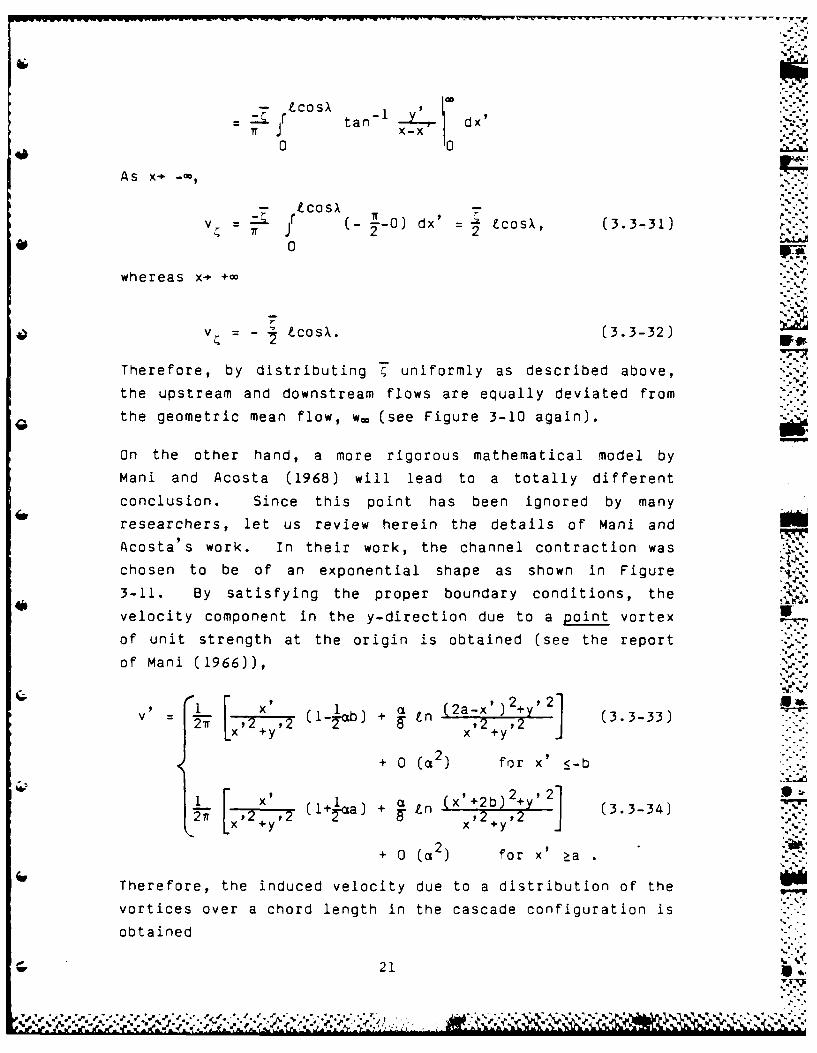
_- -O S- - - - -® - -- ' -- - --- --

- cosx 1.r tan -- I dx

W X-X0 ".

A~s x-

- cosxv=- j (- -O) dx' 2 cosX, (3.3,31)

0

whereas x- +a*

v =- -' LcosX. (3.3-32)

Therefore, by distributing c uniformly as described above,

the upstream and downstream flows are equally deviated from

the geometric mean flow, w. (see Figure 3-10 again).

On the other hand, a more rigorous mathematical model by

Mani and Acosta (1968) will lead to a totally different

conclusion. Since this point has been ignored by many

researchers, let us review herein the details of Mani and

Acosta's work. In their work, the channel contraction was

chosen to be of an exponential shape as shown in Figure

3-11. By satisfying the proper boundary conditions, the

velocity component in the y-direction due to a point vortex W

of unit strength at the origin is obtained (see the report

of Mani (1966)),

: ,2 ,2 (1-yab) + g-n 2x2,2 (3.3-33)

+x +y x +y x' ::b

22+ 0 (a) for x' <-b-x a (x9 2 ),+Y

,2,2(i+ra) + nI- +2b (3.3-34) 7',-x +Y x'2+Y '

+ 0 (2) for x' >a .>-

Therefore, the induced velocity due to a distribution of the

vortices over a chord length in the cascade configuration is

obtained

21 'S

-~~~~ ~ ~ -- - - - -- - - - --

v =fy(&) ~v' d& (3.3-35)n--c

with x' = (x-E) cosX

y = -ns + (x-&) sinX

Ea = -~cosx

b f + coX

-1n=-L (x-& 2+n s -_2ns(x-&) sinX

+ t [E-(x+&)COSXIJ 2 +n? S2 -2ns(x-&)sinX+(s-&) 2sin2 x8 2n 22_(x-&) nS -2ns(x-E) sinX

as x * ~(3.3-36)

[xi(X+E)Cosx+E12 +n? 2 -2ns(x-E)sinX+(x-&) 2sin 2x+ Ln 228(x-E) 2ns2-2ns(x- ) sinX

a s x -l +cc. (3.3-37)

Let's simplify the first term of the above integration by

defining

P no (X-E) cosx

Then

(X-F) cosx\P F, 2n=-ao [(x-&)-ns sin~J2 + (ns COWX

( x-0J cosx L

22

=(X-E) cosx *

n~ *1~ +f i n s -ins5e e

n- XE+ inir - inwi

4 From the identify (see Mellor (1959)),

n~o I = coth ei)

iX s

Vthen, rI

P = [.coth 7r L2. eiX + coth eX) (3.3-38)

Therefore,

P = ~ as x* .

as x-1 +co.

The second terms of (3.3-36) and (3.3-37) are defined,

respectively

Q * ~ Zn[E-(x+E)cosXj 2+n 2s2 _2ns(x-EJsinX+(x-E) 2Sir2Xn=- (x-E) 2+n 2s 2 2ns(x-)sinX

for x :S-1

[C+)cs+E + 22[4+*oxE Znn~ _2ns(x- )sinX+(x-) 2 iXn 2 2n ~x-E) +n 2s ?-2ns x-E) si nX

for x lThen,

F 2_ 23Q Zn + E 2E(x-O)cosx+ 4 xcos XI~E nl 2 22Jn=- (x-E) +n s- 2ns(x-&) sinXI

, S( -1

tn1 E +2E~x+0)cosx + 4 xcos X~1pn=- (x-E) sn - 2ns(x-E) sinX

23 S

1A

or

E~ _2 2E(x+0)cosX + 4 xcos 2Xasx1-c= w ,. X-C) 2+ 22 - 2ns(x-&) sinX~~ax-

E +2E(x+&)cosx + 4 xcos 2XI ~I2 22 ,as x- ~n-(X-C) +n - 2ns(x-&) sinX

From (A-11),

E _2E(x+FE)cosX + 4 xcos2 X ,as x.-~ .40 s (x-&) cosx

2 2

TE +2E(x+&)cosX +4 4 xcos Xx~ oX sx +G,

or

Q J (-2E + 4E cosX) ,as x-*

7r (2E + 4& cosX) ,as x-* +w.

Therefore,

v L & E 1- 1 b)( + -(2)(.2E +4&cosX ld&2 7r 2 2 s 8 s -

as x.-

I ~~ (1+ a ca)( + ~ . )2E + 4&co sX) dE ijj-I ,as x-l- +cc

Assuming a symmetric loading (i.e., y()d=0),

v = [I -Li (b + )] ,as x-P c

L 21 ' as x-* + _

24

bI

where Is a y( )dE and y(E) is positive in the clockwise

-1

direction. If E = 2a = 2b,

V - (I- 2E) as x-..2s 2

(3.3-40)

(+ SE) as x+

Rewriting this induced velocity in two parts, by vr, and v.,

v v as x-

where vp v rr c'E.,'W'

The velocity diagram is now written in Figure 3-12. It is

clearly seen that there exists an error of first order of a

if w. is chosen as the reference velocity. Instead, w..'

should be chosen as the reference velocity so that the blade

setting will be changed. This error is substantial since

the three-dimensional, diagonal flow correction handled

under the current method is order of magnitude a. This fact

indicates that not only the blade camber profile needs

correction as discussed earlier but also the blade setting

should be changed in order to take such 3-D correction into

account correctly. Inoue, et al. (1979, 1980) did not see

this point in their series of papers.

There exist two possible ways of implementing this idea:

I) by assessing the flow channel contraction or expansion in

terms of equivalent a, Equation 3.3-40 will be used, and

2) a more accurate calculation will be made by using the

distributed vortices over the cascade strip. The method of

actually incorporating this flow "skewness' into the curr'ent

design theory will be one of the major tasks in the FY-87 _''_

GHR project.

25

.....

3.3.7 Secondary Flow Correction

The secondary flow theory commonly used for axial flow is

applicable to the current diagonal flow. The strength of

vortex at the exit of blade channel due to the secondary

flow, rSF, is expressed

1~~~• --1 b F scd-

CSF 2 r dcos_d w )

where N = number of blades,

0 = the component of vortex normal to the directionof relative flow on the rotating surface,

w = relative incoming velocity

s = line element along the blade on the rotatingsurface

w = relative flow velocity on the blade surface

Ir = circulation of blade

q = q-line used for the streamline curvature method

= angle of a tangent line of meridional line madewith q-line

* bl, b2 = widths of flow at inlet and exit, respectively

82 = flow angle at exit relative to chord line.

By distributing the above secondary vortex at the exit of

blade channel and satisfying the boundary condition on the

hub and casing, the induced flow effect on C9 (called AC9 .4

hereafter), will be calculated by solving the corresponding

Poisson's equation. In the current design problem, this AC,

will be taken into consideration for determining the blade

profile shape. More detailed numerical analysis will be -

developed in future work.

3.4 DESIGN PROCEDURE

The design procedure presented here is based on the assump-

tion that the shape and steady velocity of underwater

26

1. 4

vehicle is given. The whole procedure can be repeated for a 0%!

modified shape or velocity. At the beginning, some parame-

ters, such as the location of the rotor, the number of

blades, and rotation speed, have to be chosen based on

experiences.

Then (Figure 3-1), the stream curvature method (SCM) is used

to determine the streamlines for a through-flow in a merid-

ional plane. As discussed in Section 3.1, the method is

based on solving the momentum equation along quasi-

orthogonal lines (q-lines) and the conservation of mass is

kept along the meridional direction.I. .. Orr

After streamlines are determined, average stream surfaces

are taken to be the revolution of streamlines about the axis

of rotation. Then a program, DSN3, is used to do the

remaining design procedure. Figure 3-13 depicts the macro

view of the procedure while Figures 3-14 through 3-18 show

details of each substep based on the theory presented inSections 3.1 to 3.3.

Figure 3-14 shows the input data required in the general

background. Input data related to each individual cross-

section are to be read in Subroutine INP2 as shown in Figure 1

3-15. Some input data are obtained from the meridional flow

solutions computed in the SCM program.

Figure 3-16 shows the subroutine to calculate the flow vel-

ocities in the mapped (X,Y) plane as discussed in Section

3.3.2. The subscripts 1 and 2 denote conditions at inlet

and exit, respectively, of a blade.S.-

One basic concept in the present design procedure is that

the blade camber design based on cascade experimental data

is adjusted, by considering the effects of streamline incli-

nation and nonuniform velocity distribution, such that both

the final flow turning angle and the incident angle relative ...

to the axis of rotation are the same as those obtained in

27 .

% . o

---- -

the two-dimensional flow without the three-dimensional fac-tors. -'-..

The camber and turning angle for the case of uniform,

parallel flow are evaluated based on the required lift coef-

ficient and solidity (Figure 3-17). The method relies on

the experimental data presented in Section 3.2.2.

In the presentation of three-dimensional effects, which are

to be considered in the boundary condition as discussed in

Section 3.3.5, the camber and stagger angle are adjusted

until the turning angle in the mapped two-dimensional plane

is the same as that with original camber in the uniform,

parallel flow (Figure 3-18). A linearized cascade theory

(Section 3.2.1), together with proper boundary condition

which has the three-dimensional effects considered (Section3.3.5), is used to calculate the cascade lift coefficient

and the associated total circulation.

If the calculated turning angle for the three-dimensional

flow case is different from the desired value, the camber

and stagger angles are adjusted in an iteration process

until the desired value is achieved to within certain

tolerance criterion. When the result is converged, the V

final camber is the one which, under the influence of three-

dimensional flow, will yield the desired lift coefficient.

V

28"OS

4.0 CONCLUSIONS

During the FY-86 GHR study, the mathematical model of the

blade-to-blade theory for the three-dimensional pumpjet flow

has been developed. The stream surface of nonuniform

thickness in the diagonal flow was mapped into plane by a

functional mapping function. The rotor blades now become a

row of blades, i.e., cascade configuration. The Laplace 1-7

equation in the three-dimensional coordinate system is then

converted into a Poisson s equation. This Poisson s

equation is solved as the corresponding Laplace equation

combined with the source/sink and vortex distribution on the 3'

rotating flow field as a correction. More specifically, the

two-dimensional cascade solution is corrected in terms of

blade camber profile shape due to the induced velocities

generated by the source/sink and vortex distribution. An I'"

iteration procedure is necessary to satisfy the boundary

condition on each blade, namely, the flow tangency con-

dition since the original two-dimensional cascade solution

will not satisfy the tangency condition after the correction

is made.

An additional important correction due to the correction by

the singularity distribution, particularly by the vortex S

distribution, is that of flow skewness. It seems that this

point was ignored by most researchers, but is as important

as the camber correction. It is of first order of three

dimensionality. This skewness changes the flow directions

at upstream and downstream in the same direction so that the

blade setting should also be changed. It means that the

stagger angle of the cascade blade should be changed prop-

erly

During the FY-87 GHR study, these two theories, i.e., bl.ade-

through flow theory (i.e., Streamline Curvature Method) and

blade-to-blade flow theory, will be combined and the itera-

tion procedure will be established. After developing com-

puter codes, a sample pumpjet design will De attempted.

29

I. _______

5.0 REFERENCES

Abbott, I.H., ano von Doenhoff, A.E., 1959, Theory of Wing

Sections, Including a Summary of Airfoil Data, DoverPublications, Inc., New York, NY. :

Bruce, E.P., Gearhart, W.S., Ross, J.R., and Treaster, A.L.,1974, The design of pumpjets for hydrodynamicpropulsion, Fluid Mechanics, Acoustics, and Desigr of

Turbomachinery, Part I, NASA SP-304, 795-839.

Furuya, 0., and Acosta, A.J., 1973, "A note on the calcula-Ition of supercavitating hydrofoils with rounded noses,"Journal of Fluids Eng., ASME, 95, 221-228.

Furuya, 0., and Chiang, W.-L., 1986, "A new pumpjet designiv ____ __"____

theory," Report No. TC-3037, Tetra Tech, Inc., Pasadena,CA.

Furuya, 0., Chiang, W.-L., and Maekawa, S., 1984, "A hydro-dynamic study of the ALWT (MK-50) pumpjet," Tetra TechReport TC-3725, Tetra Tech, Inc., Pasadena, CA.

Herrig, L. J ., Emery, J.C., and Erwin, J.R., 1951,"Systematic two-dimensional cascade tests of NACA65-series compressor blade at low speeds", NACA RM L51G31,National Advisory Committee for Aeronautics, Washington,D.C.

Inoue, M., Ikui, T., Kamada, Y., and Tashiro, M., 1979, "6Adesign of axial-flow compressor blades with inclinedstream surface and varying axial velocity," Bulletin ofthe JSME, 22(171), Paper No. 171-4, 1190-1197.

Inoue, M., Ikui, T., Kamada, Y., and Tashiro, M., 1980, "6Aquasi three-dimensional design of diagonal flow impellersby use of cascade data," IAHR Symposium 1980, Tokyo,403-414.

Mani, R., 1966, "Quasi two-dimensional flows throughcascades," Ph.D. Thesis, California Institute of

Technology, Pasadena, CA.

Mani, R., and Acosta, A.J., 1968, "Quasi two-dimensionalflows through a cascade," Journal of Engineering forPower, ASME, 90(2), 119-128.

Mellor, G.L., 1959, "An analysis of axial compressor cascadeaerodynamics; Part I, Potential flow analysis withcomplete solutions for symmetrically cambered airfoil "

families; Part II, Comparison of potential flow resultswith experimental data", Journal of Basic Engineering, 81,362-378 and 379-386.

30

7I

von Kdrmdn, Th. , and Burgers, J.M. , 1963, "General aero-dynamic theory-perfect fluids, In: Durand, W.F. (ed.),Aerodynamic Theory, Volume II, General Aerodynamic Theory,

4p Perfect Fluids, Division E , 1-367, Dover Publications,Inc. , New York, NY.

Weinig, F.S. , 1964, "Theory of two-dimensional flow throughcascades", In: Hawthorne, W.R. (ed.), Aerodynamics ofTurbines and Compressors, Section 8 , 13-82, Princeton

*University Press, Princeton, NJ.

Wislicenus, G. F. , 1965, Fluid Mechanics of Turbomachinery,Volumes I and II, Dover Publications, Inc., New York, NY.

OFF

31

* FIGURE 1-1 A typical pumpjet blade andshroud configuration

.r

of shroud

- .4

1 32

. ..

0.42

0.38 Free vortex

0.34

\FrV,0U .3 Forced4f vortex

E0.26

0.22

0.0 0.2 0.4 0.6 0.8 1.0 1.2

ye /V

FIGURE 1-3 A typical load distributionin terms of Va4 for puxnpjetrotor blade where V- is cir-cumferential component ofthe turned flow velocity

33

IA.-

IA-

J-

Ij//

Z

(b

FIUE1- yialpmjt oo laecn

fiuain (a to-ie n

9 (-b) upsteamvi-

'r a. / 34

%I

START~~Input ,Data o Size of Underwater Vehicle and its Drag

o Upstream Flow Velocity Profileo Goal Speed

0 Global Pumpjet* Hydrodynamic rw

Calculations

Determination o Channe Geometryof Input Data ......... o Rotation Speedfor Design 0 Head jg

Determination ofBlade-Through Flow Stream Surface by(Streamline Streamline CurvatureCurvature Method) Method with Blade

Loading and Thick-ness Assumed

Ba e-to-Blade owBlade-to-Blade Flow with Three-Dimensional

Effects incorporated--Determination ofBlade Profile Shape

~ChangeI of Loading

Distribution/ Yes

Change U

of Slade Yes

SNo''W

:Z: END

FIGURE 3-1 Flow Chart of the SelectedPumpjet Design Method

%35

is

W,,w f ?.

f t.

F Evt i

"36

m ft'.

I.f-ft

t.'!

ft ,

ft,

FIUE -'ftniin igrm.'

36 .'

- - ----------------

65 1 a4 1 0 IZ------------------------------------------

K GO-2010

* 6S-i24*IO41-MIC

or 0, 1-, - .0-

44

FIGURE 3-3 Variation of design angle of attack withsolidity for the sections tested

'p 37

28

~24-U

0 -7

-j~

z

U-j

f Ia I4 8 2i 02

4W DSIG ANLE F ATAC -4

FIUE34 Cmaio fdsg nl fatcobaie frmtemlipergeso

analsis nd tose btaied fom te 7

labraor

I I I I 38

2.8

-Beta~ 30 deg

2.4

0I.4

0.06 1.0

- o cr = 1. 2

#~ = 1.2-. 4.

.40. . 0

CPSCI10 L.IFT COEFFICIENT

FIGURE 3-5 Camber as a function of cascade liftcoefficient and solidity obtained fromregression analysis data (solid line)compared with original data (discretedata point) , for ~l=300

39

2.8

Beta~ 45 deg

2.4

2.0-

-0 1.2 -

0.4-

0.4 + a 0.5

x y= 0. 75

0.0 * a =1.o a=l1. 25# a = 1.5

-. 4 .

li0.0 0.4 0.8 1.2

CASCAD LIFT COEFFICIENT

FIGURE 3-6 Camber as a function of cascade liftcoefficient and solidity obtained from0regression analysis data (solid line)compared with original data (discretedata point), for ~l=450 ..

40

2.8

Beta -60 deq

2.4 -.

2.0 -

0.8-

0.4-+ a=0.5

*x a = 0.750. 0 = a1.0

o a =1.25-.4# a = 1.5 '

0.0 0.4 0.8 1.2

CPSCAD LIFT COEFFICIENT 7'j.*-j

FIGURE 3-7 Camber as a function of cascade liftcoefficient and solidity obtained from

regression analysis data (solid line) 7compared with original data (discretedata point), for 81 600

41

%%

2.8 -

Beta - 70 deg

2.4 -

2.0

,'°,

0.4 - 0

• o = 1 . 00.0 .o a 1.25

- ~~# = 1.5 _ .-

-.4 I I I0.0 0.4 0.8 .2

CPSCAD LIFT COEFFICIENT

FIGURE 3-8 Camber as a function of cascade liftcoefficient and solidity obtained fromregression analysis data (solid line)compared with original data (discrete 2data point), for = 700

42 I'_

- i. ,,

i Raaial direction

SMS

FIGURE 3-9 Axisymmetric stream surface

0 43

**L

upstream

VP

downstream0 **X

FIGURE 3-10 Blade setting in themapped plane

44

* E

z.

--~ a

lphe"l he ax t~.1~h - I- e

0

2cosX

FIGURE 3-11 Flow configuration infW

45 p

4WS

r-

Vr

_r

FIGURE 3-12 Flow skewness on the velocitydiagram due to vortex distribution

46

(PROGRAM DSNN3)

[ ~SUBROUTINE INP MPK.-.

I SUBROUTINE INP21.,

SUBROUTINE MAP32

SUBROUTINE DSN2

SUBROUTINE PRM31 W4

* .V

K c e NO o - K = K 1 "d

Figure 3-13 General flow chart to designblade in a flow of three-dimensional character

I"-

* 47

WW U~

Input Required lift coefficient C o

Flow vel. VO

Rotational speed RPM

Convergence criteriafor 4 eq and ABa

Max. iteration number M

No. of blades Nblad e

No. of cross-sections alongthe radius direction N

csec

No. of segments along a chord Nseg

Ref. radius ro

For K = 1 to Ncsec

Input Solidity a(K)

Peripheral vel. at inlet C (K)

Peripheral vel. at exit C 2 (K)

!-Evaluate angular vel. of rotor, w, from RPM - ..

Ref. vel. uo : row

RETURN

Figure 3-14 Flow chart for Subroutine INP

48

(SUBROUTINE INP2)

For each cross-section K,

For I = 1 to Nseg,Input Radius r(I)

Meridional vel. C (I)mDistance between adjacent

streamlines b(I)

Blockage factor Kb(I)Let relative meridional vel.wi

(I) () *

M m

4 0 At the inlet of blade,

r r(1), Cm1 Cm (1)

At the exit,

fbr 2 *r(Nseg), Cm2 *CM(Nseg)j

CRETURN

Figure 3-15 Flow chart for Subroutine INP2

VP.

GO 49

(SUB ROUT INE-MAP32-

Find w X1, w X2 1 WY1, wY2 1 w.1from Eqn. (3.3-7)

lbFind w I1( +w2- (Xl X2 U.;

Y Vi Y2 ~ ~

Figure 3-16 Flow chart for Subroutine MAP32

Is

50

Sd.~~~~ hill .~~a

(SUBROUTINE OSN2)

Determine 1 and 82 based on

tan 8=w/w

Determine camber Cb and flow angle a

from multiple regression analysis

based on experimental cascade data

CRETURN)

Figure 3-17 Flow chart for Subroutine DSN2

5A1e

51

( SUBROUTIEPM

Prepare initial turning angle C(1)

flow angle at inlet 81

40mean flow angle BOO

stagger angle

camber

*Set initial counter M

M=M + 1

Determine induced velocities and

use a 2-0 cascade theory (Sec. 3.2.1)

to evaluate the total circulation and

find the resultant turnina an le E(M)

(1) (M)

YesNo

-P 't e u 1t s A dj)u s t cambe r andp

Figure 3-18 Flow chart for Subroutine PFM3

c 52

N~

W n~ ~- '- -.

ij

N

p

* V

'I

H