,/i! = r o attitude estimation signal processing: a first ... · technical repo_ nag8-1342...
TRANSCRIPT

Technical Repo_
NAG8-1342 Supplement 1
UAH Account: 5-34744
April 1, 1997 - March 31, 1998
.,/i! = r
O
Attitude Estimation Signal Processing:
A First Report on Possible Algorithms and Their Utility z--J
/
' July 7, 1998
Prepared by: Vahid R. Riasati
Visiting Assistant Professor
Electrical Computer Engineering Department
The University of Alabama in Huntsville
Huntsville, Alabama
https://ntrs.nasa.gov/search.jsp?R=19990024885 2018-08-18T08:21:23+00:00Z

Introduction ...................................................................................................................... 1
Preconditioning ................................................................................................................. 2
Interpolation ...................................................................................................................... 4
Constant Thresholding ....................................................................................................... 5
Variable Thresholding ....................................................................................................... 6
Time Windowing ............................................................................................................... 7
Low-Pass Filtering ............................................................................................................. 9
Linear Estimation and Wiener Filtering .................................... . ......................................... 11
The Remaining Work ......................................................................................................... 15
Appendix .......................................................................................................................... 16

Introduction
In this brief effort, time has been of the essence. The data had to be acquired from
APL/Lincoln Labs, stored, and sorted out to obtain the pertinent streams. This has been a
significant part of this effort and hardware and software problems have been addressed with
the appropriate solutions to accomplish this part of the task.
Passed this, some basic and important algorithms are utilized to improve the
performance of the attitude estimation systems. These algorithms are an essential part of the
signal processing for the attitude estimation problem as they are utilized to reduce the amount
of the additive/multiplicative noise that in general may or may not change its structure and
probability density function, pdf, in time. These algorithms are not currently utilized in the
processing of the data, at least, we are not aware of their use in this attitude estimation
problem. Some of these algorithms, like the variable thresholding, are new conjectures, but one
would expect that someone somewhere must have utilized this kind of scheme before. The
variable thresholding idea is a straightforward scheme to use in case of a slowly varying pdf,
or statistical moments of the unwanted random process. The algorithms here are kept simple
but yet effective for processing the data and removing the unwanted noise. For the most part,
these algorithms can be arranged so that their consecutive and orderly execution would
complement the preceding algorithm and improve the overall performance of the signal
processing chain.
In any signal processing scenario, the utilization of particular algorithms are justified
by evaluating the specific conditions of the data and the effort. In the current scenario, the
overall goal is the development of some basic algorithms for pre-processing of data. These
algorithms include a raw data thresholding at a constant threshold that would take out any
extreme values that are just not expected to occur in relation to the other data samples in the

2
attitudecontrolsignal.Thiscanbefollowedby a time windowing to reduce leakage problems
from data segmentation, followed by a more fine-tuned thresholding scheme, perhaps similar
to the variable thresholding scheme alluded to earlier. The result of this processing should
reduce a significant amount of noise and clutter. At this point one could apply a frequency
windowing scheme to limit the throughput information to that of the signal bandwidth
estimate. Since signal precision information is of extreme importance in this scenario, on e may
want to limit the frequency of the signal by a window that has a cut-off frequency at a higher
frequency than the bandwidth of the signal. This cut-off frequency information can be specified
to the filter and the stopband for the filter can be adjusted for each particular signal. In the
simulations a prompt is utilized that asks for the signal bandwidth information and the type
of frequency limiting that is desired. These basic algorithms make up the pre-processing chain,
a step towards the actual main stream processing of the data a linear estimator is also
implemented for use with a Wiener filter to help extract the signal from the noisy and
corrupted data.
Preconditioning
In all that follows the DC440200029star data, converted from quaternian format to x,y,
and z coordinates, has been used. Prior to using the data the first and the last 425 samples are
removed. By observing the data it has been determined that these data points should not be
included as part of the data collection events due to transient effects of the system prior to the
data collection event. The remaining data is loaded into the smallest array that can contain
the data samples and is an integer power of two. The use of array sizes that are integer powers
of two helps in processing time and is useful in the implementation of some signal processing
algorithms. Figure (1) shows the original data, the chopped-off data, and the data in the
smallest power of two array that would hold the data after 850 samples are removed.

_gnaJ X,Y, Z Oata <:::_oped_ffX. Y.Z Oata1 , , , I , , ,
,< 05 ...... ;, :_:F: : o5 i:: i: ;_::'lii
"Sme "t1E ]_me
>-0.5 ;' \ ...............:i!
,.., ;_.',._........................
l I I
3.4795 3.48 3.4805 3.481 3.4815"Sme x 10s
t ..... -::_ _ i:_:i_ ii'_- ................ •
TimeI
I I I
• 3.48 3.4805 3.481Tree
\ \l" \ _17
3.481 3.4815
X15
34815
xt_
1
(a) (b)C_of_oe_-olfData_t_ Powa"otTwoAn'aySize DataWiOlout_tsBas
1 .... , , ,
. _._,._._...... !. x j - ---.-_Lc.;: ;_.::. ,_._;::_;_::_
" " ° " ...........i i" ..........i i I i I I I I i
3.4796 3.4798 3._18 3.4_02 3,4804 3.4_ 3.4_8 3.481 3.4812 " 3.47963.4798 3.48 3.4802 3.4804 34806 3.4_ 3481 34812
t t....>- 05 :' _+.i iiii_il]iiil ': >- =,=,_:_ :. ==,,,,_;'.,_.,:::., .......
: - .-0,5
304}94 :' ..... ; ....... 3.4796 3.4798 3.48 3.4802 3.4804 3.48C6 3.4808 3481 34812 3"._ 3.47963.4798 3.48 3.4802 3.4804 3.4806 3.4808 3.481 34812
1 .... 13me . , ,_Id , T_e .... _'1_
_'3. _ _=,_" "....... _' _,_____,_ i-J'_,, , , , , Jl4 3.4796 3.4798 3.48 3.4802 3.4804 3.4806 3.4808 3481 34812 3"4794 34796 3.4798 3.48 3.4802 34804 34806 3.4808 3.481 34812
"_me x I_ T_'ne x I0_
(c) (d)
Figure(I), (a) The original coordinates in X, Y, and Z, (b) the data after removal of transient
data that is not part of the data collection event, (c) the data after it has been placed in an
array that is a the smallest power two which can contain this data, (d) the data after the
constant bias has been removed.
3
To work with the data more effectively and be able to observe the relative magnitude
of each of the frequency components of the signal more dearly, the dc bias of the data is
removed.Theconstantbiasinformationis ingeneraloflittleuseinsignalprocessingscenarios
sincethis informationrelates to no variation in the signal. Hence, all that is really needed is
the actual value of the bias so that it can be added back to the signal at the end of the
processing chain. The constant bias is added back in to the signal because for most electronic
circuits the signal is useless unless the correct bias level is used. Ultimately, the goal is to
recover the original command signal from the noisy and corrupted data; this includes the bias
and relative delays of the data. Most of the algorithms, with the exception of the Linear
Estimator and Wiener filter, presented here can be thought of as preludes to the actual signal
recovery and estimation algorithms.
4
Interpolation
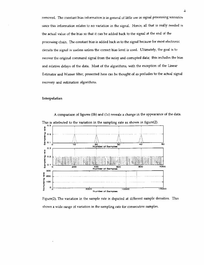
A comparison of figures (lb) and (lc) reveals a change in the appearance of the data.
This is attributed to the variation in the sampling rate as shown in figure(2).O.3
c_ 0.2 ................. _ ................ , ................. _................. ', ...............
i
0_ 0 10 20 30 40 50
Numbor of Samples
0.3 _ _ _ L |
:i*, .... _:'"" *'"'; "1 " iili
0 0 200 400 800 800 1000Number of Sampl_
3OO
l , i
e
0
C 100
o 5o00 _o&o __oooNumber of Samples
Figure(2), The variation in the sample rate is depicted at different sample densities. This
shows a wide range of variation in the sampling rate for consecutive samples.

Thedatapresentedin this report is not sampled at a regular spacing. The relative
sample spacing for consecutive samples shown in figure (2) indicates this clearly. This
irregularity implies that some type of curve fitting or interpolation must be utilized to estimate
the necessary samples that are missing. This problem is significant and should be addressed
prior to the actual implementation of the simulated algorithms that are discussed in this
report.
Constant Thresholcling
To provide basic removal of unlikely noise events a constant thresholding has been
implemented to remove data events that are three standard deviations above the standard
deviation, SD, of the data. A constant pdf is assumed for the SD calculation of the data. This
is justified by noting that there are a number of processes in this data and some of these
processes are changing with time; these processes are usually smooth and decreasing as the
random variable moves away from its mean value, or at worst the probability of the event
occurring will remain constant as the random variable moves away from its mean. Even if the
pdf were constant for a random variable, the mere fact that there are several additive random
variables in this data would imply, by the central limit theorem, that the pdf of the sum of
these variables will fall off as variable's values move away from the mean value. Hence, by
calculating a generic SD for the data using a constant density and a threshold value that is two
or three times larger than this SD unlikely events that would follow any usual density should
be removed from the data. This is a good first attempt at thresholding, because the chances
that this process would remove any of the command data are extremely small. This is due to a
high threshold relative to the variation of the data and the increase in the possibility-of-
occurrence for highly unlikely events in the moment calculations through the use of a constant
pdf.

×
0.5
Data After Constant Thresholdlng
...I ............................... - ...... ".-=-:"':i:_:_:_iL_ ::!_i
--0.5 J i i i i i i3.4794 3.4796 3.4798 3.48 3.4802 3.4804 3.4806 3.4808
Time
-o._°'°_ f i ...............' i ..........- l i''_'ii [ if::::i!i::_[ti_ =':'_"r_'':;' ..................'.....L-1 i =
3.4794 3.4798 3.4798
1
NO
-1 i t i3.4794 3.4798 3.4798 3.48
i3.481 3.4812
x l_J _
i i i i i
3.48 3.480.F.364804, 3.4806 3.4808
i i i i
3-480._m3o4804 3.4806 3.4808
...................
i3.481 3.4812
tt') e
3.481 3.4812X 10 e
Figure(3) (a) The data after constant thresholding. STD_X=0.2317,
STD_Y:0.3559, STD_Z=0.4200; Thl=3.*STD_X;Th2=3.*STD_Y;
Th3=3.*STD_Z;
Variable Thresholding
The variable thresholding starts with the assumption that most random processes are
not stationary and change in time. So, the idea of a wide-sense stationary process can be used to
calculate the standard deviations along windowed segments of the data. In other words,
adjustable segments in the temporal data are utilized on the basis that relative to the
windowed segments of data the variation of the noise structure is slow and is not significant
over the window where the first and the second statistical moments are being calculated.
The size of the window is chosen rather arbitrarily for the examples used in this
report, however, this choice must include the sampling rate, or in other words the largest
frequency component of the signal. The current results are obtained with sliding windows that
contain 10 samples. Figure (4) shows the results of applying the variable thresholding idea to
the data, along with the variation of the SD of the data. The variation in the SD of the data

isprovidedasan instructive measure to help in communicating the relative change in the
variance that is utilized in thresholding the various windowed segments as the algorithm
progressively includes new samples. A basically flat plot for the SD would imply that
variable thresholding should not be used.
1 . 1 Data,AlterVala_e, Thresaoldng.... x 0.4.]o: t t........ _ :i_::i _'0.2
3.4794 3.4796 3.4798 3.48 3.4802 3.4804 3.4806 3.4808 3.481 3.4812
............. .................] o2[i>" "............ _ I
.I -l l r l I J J i 0 L,
3.47943.47963,47_ 3.48 3.480_3.48043.48C63.48083.4813.4812
I
, , ,,_:=_A..... E............. , l" i! i N o,2
3"_794 ......... 3.48 3.4812 !\3.4796 3.4798 3.4802 3.,18043.4806 3.4808 3.481 0/,
xl0a
StandardDevi_onVa_af_on
2000 4000 O000 8000 10(]00 12000 14000
, Slidi_ Win<_ , ,
2OOO
I40OO 6OOO 8OOO I00_ 12OOO
SlidingWindow14OOO
......_.i:Cili_iii!i_,_40O0 60OO 80)0
SlidingWindow
I
il,I
10000 12900I
200O 14(_0
(a) (b)
Figure(4) (a) The data after variable thresholding of window size ten is applied to the data
(b) the variation in the standard deviation of the data over the progressive ten sample
windows.
Time W'mdowing
The purpose of data windowing is to modify the relationship between the spectral
estimate Pk at a discrete frequency and the actual underlying continuous spectrum P(f) at nearby
frequencies. In general, the spectral power in one '_bin" k contains leakage from frequency
components that are actually s bins away. This is due to the limitation that is put on the
function by the finite size of the FT window. There is quite substantial leakage even from
moderately large values of s.
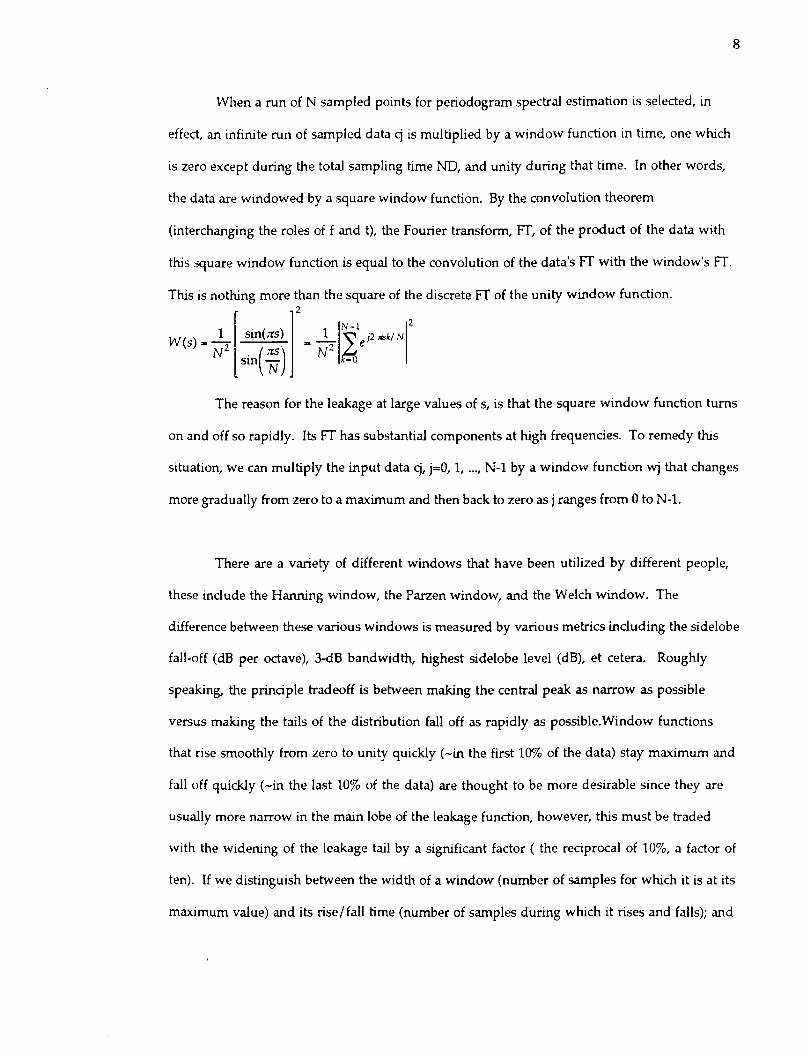
Whenarunof N sampledpointsfor periodogramspectralestimationisselected,in
effect,aninfiniterunof sampleddatacjismultipliedbyawindowfunctionin time,onewhich
iszeroexceptduringthetotalsamplingtimeN-D,andunityduringthattime. In otherwords,
thedataarewindowedbyasquarewindowfunction.Bytheconvolutiontheorem
(interchangingtheroles of f and t), the Fourier transform, FT, of the product of the data with
this square window function is equal to the convolution of the data's FT with the window's FT.
This is nothing more than the square of the discrete FT of the unity window function.2
W(s)
[s'nt'd)
The reason for the leakage at large values of s, is that the square window function turns
on and off so rapidly. Its FT has substantial components at high frequencies. To remedy this
situation, we can multiply the input data cj, j=0, 1, ..., N-1 by a window function wj that changes
more gradually from zero to a maximum and then back to zero as j ranges from 0 to N-1.
There are a variety of different windows that have been utilized by different people,
these include the Hanning window, the Parzen window, and the Welch window. The
difference between these various windows is measured by various metrics including the sidelobe
fall-off (dB per octave), 3-dB bandwidth, highest sidelobe level (dB), et cetera. Roughly
speaking, the principle tradeoff is between making the central peak as narrow as possible
versus making the tails of the distribution fall off as rapidly as possible.Window functions
that rise smoothly from zero to unity quickly (-in the first 10% of the data) stay maximum and
fall off quickly (-in the last 10% of the data) are thought to be more desirable since they are
usually more narrow in the main lobe of the leakage function, however, this must be traded
with the widening of the leakage tail by a significant factor ( the reciprocal of 10%, a factor of
ten). If we distinguish between the width of a window (number of samples for which it is at its
maximum value) and its rise/fall time (number of samples during which it rises and falls); and

if wedistinguishbetween the FWHM (full width to half maximum value) of the leakage
function's main lobe and the leakage width (full width that contains half of the spectral
power that is not contained in the main lobe); then these quantities are related roughly byN
FWHMinbins--windowwidth
9
N
Ieakagewidthinbins~ windowrise, falltime
Figure(5) shows a variation of the Welch window which is used in the
simulations.
0.8 --7 ....................... ',- ........
0.6 • -............................... :........
0.4 ............................ _........
0.2 ............................. - ......
°o _xlO 4
0.4
Data After Temporal Windowing
1
.......... Ili!_i_....................0.5 +!'_: !i!| ,
o ...... _::::':"_':!....... !:,.............
_ I2 °3s._79 3._ 3.@1 3.482Time x 106
02 .......... igIi++::::+....:.........../ii::::_Hl_tili :
o ...... .,_--- i+:i++Jll_i.':,_.... i..... , ......
-0.2 ....... +.............. !- • -, : -_..........
-0.4 ............. : ........... _il ..........i<':r
-0.6 _'3.479 3.48 3.481 3.482
Time x 10 a
0.5
N
0
-0.53.479
.......... it+I,".._:.... :: {: ...........
_ :!l!:i::: i '_ : '::L
..... " .... O ,.:_......... t;..-- .........
1F_._f +
3.48 3.481 3.482Time x 1 06
Figure(5) Top left to bottom right: Window, X-data, Y-data, and Z-data
after windowing.
After removing the mean of the data, the power spectrum should contain a large signal at a low
frequency, then small signals centered at progressively higher frequencies, the noise. These
small signals are what we would like to eliminate.
Low-Pass Filtering

10
Windowing the data in the frequency domain can make it smoother than it is now by
removing some of the high frequency data. This is sometimes referred to as low pass filtering.
Remember, however, that only a minimal range of the highest frequency information should be
filtered out. This can be done by implementing a frequency windowing scheme with an
adjustable cut-off frequency. One such window is a simple triangular function given by,
f(w)=l-f w I for -1<w<1;
= 0 elsewhere
where w is a normalized frequency. A variation of this is to allow I w l to take on powers
higher than one. This will reduce the amount of high frequency information that is allowed,
while increasing the magnitude of the low frequency contents of the data. The slope of the
isosceles triangle relative to its base can be modified to incorporate the desired 3dB
bandwidth. Other Low-pass filters that are implemented in the simulation are the
Butter'worth and the Square filters. Figure (6) shows the frequency characteristics of a second-
order Butterworth filter and the results of its application to the data.
Low-Pass Filtering. Butterworth, w3db=500
0.8 .................................
00.6 .............. i ................
_c_0.4 ............ ,
: £
°2 ........ :0 0.5 1.5 2
Sam )les X 104
(_ 0.5,(ao
I>" 0
--_-o.5u_
-1o
.... _1 :it_ll
II
Linear Estimation and Wiener Filtering
The pre-processing algorithms that have been discussed should be followed by a series
of algorithms that attempt to recognize and extract the command signal from the noisy data.
As an example of this type of filtering algorithm a simple adaptive Wiener filter has been
implemented to reduce the undesirable noise in the data. This filter uses a best-linear-fit to
estimate the noise information and utilizes this information to extract the signal spectra from
the noise; this is used to reduce the cluttering pink-noise in the attitude data. Figure(7) shows
the results of applying the Wiener filter to the data.
Weiner Filtering X_Data
2O
10
W I
5z
00
J
...../i;:........:.:.:..............
../"............!......\........../
,f , . ' \,
0.5 1 1.5 2
Num_Samples x 10 i:
20OO
11500
,ooo
t 500c
0
.............. i ....................
A_0.5 1 1.5 2
Num_Samples x 10 !:
(a) (b)
2000
_._I 5O0
_ 500
u.
0
0.5 1 1.5
Num_Samples x 10
i
u.
1
0.5
0
-0.5
.: _'¢_:.@_ i ii ' ;..,.....
2 3.4795 3.48 3.4805 3.481 3.4815
:, Time x 10 !:
(c) (d)
Figure(7), The Linear Estimation Wiener filter results, a) the estimate used for the noise
spectrum, b) the noise and signal spectrum, c) the filtered signal spectrum, d) the signal after
filtering. Figure(8) shows the results of all three coordinate data after wiener filtering has
been applied to extract the signal.

12
Original X, Y, Z Data1[
x 0
/-13.4795 3.48 3.4805 3.481
1 _ Time
-I ,: , , _i........3.4795 3.48 3.4805 3.481
1 "l']rne
_i : i_l__'_...............
a_4795 3._,8 3.4_05 3&1Time
3.4815
x 10]
3.4815
× 10]
3.4815
x 106
Weiner Filtered X, Y, Z Data1 , ,
/-11 , J ,
3.4795 3.48 3.4805 3.481Time
>.10 . ,, ' .-,_ ' : '
.1 / i i I
3.4795 3.48 3.4805 3.4811 , Time ,
I ,,. .............. :.....
3"._1795 3.48 3.41305 3.481Time
3.4815
lOi3.4815
x 10i
3.4815
xlO 6
Figure(8), The X, Y, and Z coordinate data points are depicted prior and post Wiener Filtering.
The noise estimation can be made more sophisticated to include a more accurate model for the
variations of the spectrum. This should improve the performance of the filter. Segmentation of
the data should also help in the implementation of a more effective Wiener filter.
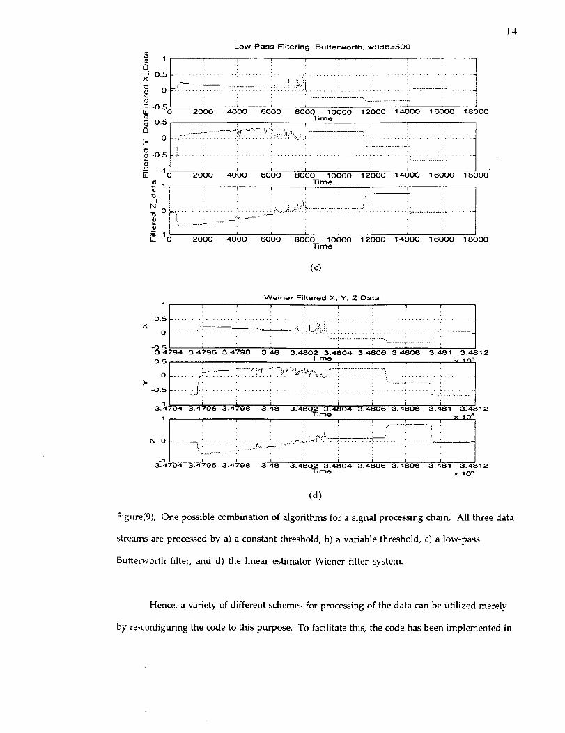
So far each of the algorithms have been applied to the original data to see the effect of
each algorithm independent of the other algorithms. Another approach to utilizing these
methods in the simulation is to implement two or more of these algorithms together, for
example, the Butterworth filter may be utilized after the constant and variable thresholding in
conjunction with the linear estimator and Wiener filtering of the data. The results of this
particular combination of algorithms are presented in Figure(9).

Data After Constant Thresholding
1 ! ! ! ! ! ' ! ! ! t....... ; ........ :.... i..i'.,'_'. J-_' ;;!_" ,"_'_:_ --; ......... ;....... ; ........ :.......
o .... _-; ....... ';-:-;:::'-. -_--'_'_'_!_'_!:_!_!:! _-- ; ........ :....... i ...... __-_
i i i ............:: ...........i.............. /_3.4794 3.4796 3.4798 3.48 3.4802 3.4804 3.4806 3.4808 3.481 3.4812
Time ",,"10 _
..... : i ,, :., ,.}I ......
2 ?_.........-0.5 _ :
-13.4794 3.4796 3.4798 3.48 3.4802 3.4804 3.4806 3.4808 3.481 3.4812
Time x 1(_
N 0 .... ==- ......... :.... :..!_.-_ }..I._ L.;!_j_J;u;'._:":............. :......... _ ..... k__ ....| • . : ',1 _,L,L-- ,
_1 1 i i i i i i i3.4794 3,4796 3.4798 3.48 3.4802 3.4804 3.4806 3.4808 3.481 3.4812
Time x 10 e
X
)-
Ca)Data After Variable Thresholdimg
0.5 ......... :. ......... :......... : ......... :......... : ......... :......... ; ....................• ' ' , • / :_,_:i, , ' " :
o .....'- .................:........._.......:__......_t::i,,,l;.,;i_ti_: : i .....;................
._._l , I I , l , , I: 794 3.4796 3.4798 3.48 3.4802 3.4804 3.4806 3.4808 3.481 3.4812Time x 1(_e
' ...............:'-:"_':q'-_P;"_:__"=_ ' ............. i_o ........ ,,/,.............. _ "_".,',, _-t ".,__!f_{'_ .......................
-o.s ...... :_:j.................... i ......... i......... i .................. _....... i:.:.i:.:.:.:.:.:.:.:..--
-1 t _8 I I I I3.4794 3.4796 3,4798 3. 3.4802 3.4804 3.4806 3.4808 3,481 3.4812Time x 1 l_ e
1 I ' , , . !!N 0 ........................ . ...... :.. :.:,_k.,_..__'_'_'_-':':':'!':':':-:-:':':':':7":':': ................
"1 I I I I I I I I
3.4794 3.4796 3.4798 3.48 3.4802 3.4804 3.4806 3.48013 3.481 3.4812Time x 10 _
13
(b)
X I
.=_
Q
>-
t.@
I.L
Low-Pass Filtering. Butterworth, w3db=500
1 / ! ! l ! ! i
o.51-I........ i.......... ...... , ........ i ....... , ........ i........ i ......... _.......
o =' ...... i .... :: :-T:::::- :--?:-::"::'_:::-_!,: ....... ! ........ } ......... i:.:m:-= _........
-0 5 _ ........" 0 2000 4000 6000 8000 10000 12000 14000 1 6000 18000
0.5 Time
I 0 t"-777 .:........... ::_..... _..' .;,_;-:i.t,;_.:,/ ........ i ...... :_:-:......... :................
j. ....::.........:..........!.... ........ ................-10 2000 4000 6000 8000 10000 12000 14000 1 6000 18000
Time
N I , , .i!,..,.'!i..............',..............: : :i .
"'x ,_ _-.-_ _'" : : : : ................. T'
•=--1 i i i i i i " ;LL 0 2000 4000 6000 8000 10000 12000 14000 16000 18000
Time
(c)
14
Weiner Filtered X, Y, Z Data
1 _ F I I I J I I
0.5 ......... L ................... ;......... :......... ; ......... :......... :......... L ........
o ....... :(: ........ ;......... : ...... .!:,_._:._!_,:!':!.i!::.... , -;%
• ""q .................. _........ : .......... . .............. i ", . . . . .
-__, , ," 94 3.4796 3.4798 3._1.8 ' ' ' 3.4808 ' 3.48123.4802 3.4804 3.4806 3.481
0.5 Time _. lt_le
-°°I.....:Ji.............................................i...............-1 I I I I I I I I
3.4794 3.4796 3.4796 3.48 3.4602 3.4804 3.4806 3.'4,B06 3._1 3.4_B12
1 Time _ 106t r i r r
N 0 ........."..................._......:_:,_!_'Y.'Tz.........._ ......................_',L................ ..........;........... '_- '
-1 i i I I i I I3.4794 3.4796 3.4798 3.48 3.4802 3.4804 3.4806 3.4808 3.481 3.4812
Time x 10 e
(d)
Figure(9), One possible combination of algorithms for a signal processing chain. All three data
streams are processed by a) a constant threshold, b) a variable threshold, c) a low-pass
Butterworth filter, and d) the linear estimator Wiener filter system.
Hence, a variety of different schemes for processing of the data can be utilized merely
by re-configuring the code to this purpose. To facilitate this, the code has been implemented in

15
a modular format and flags have been incorporated to easily allow for the selection of the
algorithms of choice. The appropriateness of the utility of these techniques depends on a
number of variables, including the statistics of the data and the random structure variation.
However, the basic algorithms are applicable to most data sets and should be useful in rejecting
and reducing noise and estimating the signal.
The Remaining Work
If one were to compare this effort to writing an essay, it could safely be said that the
outline for the essay has been done. Now, the work of writing and re-organizing the contents,
spell-checking and grammatical correctness, of the essay must begin. The body of the essay can
be compared to a series of tests of a consistent array of low-pass filters to determine their
applicability to the particular data types that are under consideration here, then the results of
these test must be evaluated with reasonable merits and the best filter(s) should be used. Of
course a set of metrics are necessary to define "best" as far as these data are concerned. A
remodeling of the noise estimation algorithm should be utilized to improve the performance of
the Wiener filter. A set of three to five analytical models should be used and tested for
performance evaluation on a set of typical attitude data sets. Similar metrics to those used for
the low-pass filter evaluation could be utilized, even thought adjustments must be made to
make the distinction between the objective function of each algorithm. Finally, a series of tests
including the "best" choices of algorithms is necessary to choose the various algorithm-sets
that are to be used in series for the over-all signal processing chain. At the end of these tests, a
series of algorithms should be chosen for use with the various data sets. Finally, since all this
falls under algorithm design and development, one should determine a global metric for the
evaluation of the entire process. One method for achieving this is to compare the final

16
estimatedcommand signal with the actual command signal, then do the same comparison with
the signal prior to any processing. A relative metric of these two comparisons would then
enable a measure of improvement which would determine the net worth of the signal extraction
and noise removal algorithms. This metric is essential because it would help in answering a
basic question that should always be asked and is often omitted in signal processing scenarios:
is the processing time, energy and cost worth the improvement that is achieved in the final
signal? The answer to this question is subjective from a signal processing point of view and has
a strong bias towards the application and purpose of the signal processing chain.
Appendix
This section contains a copy of the code that is used to simulate the relavent algorithms
discussed in this report. All of the results and figures have been implemented by the use
of this code.
%%%%%%%%%%%%%%%%%%%%%%%%%%%%%%%%%%%%%%%%%%%%%%%%%%%%%%%%%%%%%%%%%% Comment Box:
%
% This code implements some preprocessing algorithms for% for the MSX data. The "vulk data' is loaded in to the
% code and the pertinent data is extracted and the dc-bias
% is removed. After a constant thresholding algorithm the
% regional variations of the data is utilized to remove data
% samples that do not conform to the norm of the regional data
% in a statistical sense. A temporal windowing scheme is also
% implemented to reduce the frequency leakage of the window.
% Three different low-pass filters are also implemented, any
% one of which can be used to limit the high-frequency noise% input to the system. Finally a linear estimator is used% to estimate the noise in the data. This estimate is
% used to extract the signal from the noise in a Wiener filter
% approach.%%%%%%%%%%%%%%%%%%%%%%%%%%%%%%%%%%%%%%%%%%%%%%%%%%%%%%%%%%%%%%%%%%%%
% Load the data and extract pertinent i_o_a_on%

17
load DC4402029coord;
m=size(DC4402029coord,1);
clg, t=DC4402029coord(:,l);clear al;clear a2,dear a3
figure(1),subplot(311),plot(t, DC4402029coord(:,2)),
title('Original X, Y, Z Data')ylabei('X'),xlabel('Time')
figure(1),subplot(312),plot(t, DC4402029coord(:,3)),ylabel('Y'),xlabel('Time')
figure(1),subplot(313),plot(t, DC4402029coord(:,4))
ylabel('Z'),xlab el('Fime'), pause
figure(1),subplot(311),plot(t(425:m-425),DC4402029coord(425:m-425,2))
title('Chopped-off X, Y, Z Data')
ylabel('X'),xlabel('Time')
figu re(1),subplot(312),plot(t(425:m-425),DC4402029coord(425:m-425,3))
ylabel('Y'),xlabel("rime')
figure(1),subplot(313),plot(t(425:m-425),DC4402029coord(425:m-425,4))
ylabel('Z'),xlabel(_Fime'),pause%% Choose the appropriate FLAGS for each desiered operation
% FLAG=I => Perform the operation%bias_rem=l;dc_rem=0;th_c=l;th v=l;tw=0;LPF=l;Est_filter=l;
%
% Extract the size of the data and utilize an arrary that
% is the smallest integer multiple of 2 and can accept all% of the data.
%if m>2^9;
k=2^ (fix(log2(m))+l); del_t=t(2)-t(1);
kl=2^(fix(log2(m))-9);tl=zeros([k,l]);tl=[t(1):del_t:(k-1).*del t+t(1)]';else
s=_Data set is not large enough';end
al=zeros(k,1);a2=zeros(k,1);a3=zeros(k,1);al(425:m-425)=DC4402029coord(425:m-425,2);
a2(425:m-425)=DC4402029coord(425:m-425,3);
a3(425:m-425)=DC4402029coord(425:m-425,4);
figure(2),subplot(311),plot(t1,a1)
title('Chopped-off Data with Power of Two Array Size ')ylabel('X'),xl ab el(_Fime ')
figure(2),subplot(312),plot(t1,a2)ylab el('Y'),xlab el("I'ime')
figure(2),subplot(313),plot(t1,a3)ylabel('Z'),xlabel('rime'),pause%clear DC4402029coord
%% Bias Removal
%if bias_rem==l
dcl=mean(al);dc2=mean(a2);dc3=mean(a3);
al=al-dcl;a2=a2-dc2;a3=a3-dc3;
end;

%% DC Removal%
if dc_rem=--1LFR=3;AI= fftshift(fft(al));A2= fftshift(fft(a2));A3= fftshift(fit(a3));dcl=Al(k/2-LFR:k / 2+LFR);dc2=A2(k / 2-LFR:k/2+LFR);dc3=A3(k / 2-LFR:k / 2+LFR);
Al(k/2-LFR:k / 2+LFR)=zeros(size([k/2-LFR:k / 2+LFR]));A2(k/2-LFR:k / 2+LFR)=zeros(size([k/2-LFR:k / 2+LFR]));A3(k/2-LFR:k / 2+LFR)=zeros(size([k/2-LFR:k/2+LFR]));al=ifft(fftshift(A1));a2=ifft(fftshift(A2));a3=ifft(fftshift(A3));end
%
% Constant Thresholding%
if th_c==lstdl=std(al);thl=mean(al);std2=std(a2);th2=mean(a2);std3=std(a3);th3=mean(a3);for i=l:m
if abs(al(i))>=(3.*stdl), al(i)=thl; end;if abs(a2(i))>=(3.*std2), a2(i)=th2; end;if abs(a3(i))>=(3.*std3), a3(i)=th3; end;end
figure(4),subplot(311),plot(tl,al)title('Data After Constant Thresholding')ylabel('X'),xlabel('Time')figure(4),subplot(312),plot(t1,a2)ylabel('Y'),xlabel('Time')figure(4),subplot(313),plot(t1,a3)ylabel('Z'),xlabel('Time'),%pauseend;%
% Adaptive Thresholding Using Absolute Values%
if th_v==l1=1
rss=10;
for j=1:1for i=rss+l:m-850
al_temp=al(i-rss:i);a2 temp=a2(i-rss:i);a3 temp =a3(i-rss:i);if abs(al(i))>=(thl+0.05.*thl.*stdl_temp(i)), al(i)=thl; end;if abs(a2(i))>=(th2+0.05.*thl.*std2_temp(i)), a2(i)=th2; end;if abs(a3(i))>=(th3+0.05.*thl.*std3_temp(i)), a3(i)=th3; end;end;
figure(5),subplot(311),plot(tl,al)title('Data After Variable Thresholding')ylabel('X'),xlabel('Time')figu re(5),subplot(312),plot(t1,a2)ylabel('Y'),xlabel('Time')figure(5),subplot(313),plot(t1,a3),% pause,ylabel('Z'),xlabel(_ime')
stdl_temp(i)=std(al_temp);thl= mean(al(i-rss:i));std2_temp(i)=std(a2_temp);th2= mean(a2(i-rss:i));std3_temp(i)=std(a3_temp);th3= mean(a3(i-rss:i));
18

19
figure(6),subplot(311),plot(stdl_temp)title('Standard Deviation Variation')
ylabel('STD X'),xlabel('Sliding Window')
figure(6),subplot(312),plot(std2 temp)ylabel('STD_Y'),xlab el('Sliding Window')
figure(6),subplot(313),plot(std3 temp)
ylabel('STD_Z'),xlabel('Sliding Window'),pauseend
end;
%% Temporal Windowing%if tw==l
11=1
for l=l:k;
window(1)=l-(((1-1)-.5.*(k-1))./(0.5.*(k+1))).A6;end;
figure(7),subplot(221),plot(window),grid
al=al.*window';
a2=a2.*window';
a3=a3.*window';
figure(7),subplot(222),plot(t1,al),grid
ylabel('X'),xlabel('Time')
figure(7),subplot(223),plot(t1,a2),grid
ylabel('Y'),xlabel('Time')
figure(7),subplot(224),plot(tl,a3),grid
ylabel('Z'),xlabel(_Fime'),pause
gtext('Data After Temporal Windowing')end;%% Low-pass filtering: 1) Square, 2) Triangular, 2) Butterworth%if LPF==I
w3db=input('what is the 3dB cutoff (in _of samples) for the filter '),
s=input('Which LPF would you like to use?(square, triangular, butterworth) ','s')
LPS=strcmp(s,'square')
LPT=strcrnp(s,'triangular')LPB=strcrnp(s,'butterworth')111=1
% Low-Pass FilteringY=zeros([1,k]);if LPS==I
Y(k/2-w3d b:k / 2+w3db)=l;
end;if LPT==I
Y(k/2:k/2+2.°w3db)=1-(1./(2.*w3db)).*[0:2.*w3db];
Y(k/2-2.°w3db:k/2)=(1./(2.'w3db)).°[0:2.*w3db];end;if LPB==I
for i=l:k
Y(i)=l./(1+((i-k/2)./w3db).^4);

end;
end;
figure(8),subplot(221),plot(abs(Y)),grid
ylabel('Window'),xlabel('Samples')
A1 = fftshift(fft(al));A2=fftshift(fft(a2));A3=fftshift(fft(a3));a=ifft(fftshift(Al.'(Y'.^l.0)));
aa=ifft(fftshift(A2.'(Y'.^l.0)));
aaa=ifft(fftshift(A3.'(Y'.^ 1.0)));
figure(8),subplot(222),plot(real(a)),grid
ylabel('Filtered X_Data'),xlabel(_Fime ')
figure(8),sub plot(223),plot(real(aa)),grid
ylabel('Filtered Y_Data'),xlabel(_ime')
figure(8),subplot(224),plot(real(aaa)),grid
ylabel('Filtered Z data'),xlab el('rime')
gtext(_Low-Pass Filtering, Butterworth, w3db--500')
figure(8),subplot(311),plot(real(a)),grid
ylabel('Filtered X_Data'),xlabel(_Fime ')
figure(8),subplot(312),plot(real(aa)),gridylabel('Filtered Y_Data'),xlabel('Time')
figure(8),subplot(313),plot(real(aaa)),grid
ylabel('Filtered Z_data'),xlabel('rime')
gtext(_Low-Pass Filtering, Butterworth, w3db=500')
pauseend;%
% Estimation and sub-optimal (Wiener) filtering%noise estPSD=zeros(k,1);
index=[0:k/2-1];
if Est_filter==lff LPF==I
Al=fftshift(fft(a));A2=fftshift(fft(aa));A3=fftshift(fft(aaa));
w3db_Est=w3db;else
w3db_Est=input('what is the 3dB cutoff (in _tof samples) for the Est_filter '),AI= fftshift(fft(al));A2= fftshift(fft(a2));A3=fftshift(fft(a3));
20
end;
sd=sum(abs(Al(w3db_Est:k/2)));
sdi=sum(abs(Al(w3db_Est:k / 2)).*abs(index(w3db Est:k / 2)'));
si=sum(abs(index(w3db_Est:k / 2)));
sii=sum(abs(index(w3db_Est:k / 2)).* abs(ind ex(w3db_Est:k / 2)));
beta=(sdi-si.*sd)./(sii-si.^2);
alfa= sd-((sdi-si.* sd)./(sii-si.A2)).*si;
noise estPSD(l:k/2)=alfa+beta.*index;
noise estPSD(k / 2+1 :k)= noise_estPSD(k / 2:-1:1 )';
figure(9),subplot(221),plot(abs(noise_estPSD)),grid
ylabel('Noise_Est Spectrum'),xlabel('Num_Samples')
sig_estPSD=sqrt(abs(Al.*conj(A1)-(noise_estPSD.a2)));
figure(9),subplot(222),plot(abs(sig estPSD)),grid
ylabel('Signal_Est Spectrum'),xlabel('Num Samples')
fi I sig_PSD=(( A1 )). / ( 1+((noise_estPSD)./(sig_estPSD+0.1 )));
figure(9),subplot(223),plot(abs(fil_sig_PSD)),grid
ylabel('Filtered_Signal Spectrum'),xlabel('Num_Samples')

signall=ifft(fftshift(fil_sig_PSD));
figure(9),subplot(224),plot(tl,real(signa11)),gridylabel('Filtered_Signal'),xlabel('Time')
gtext('Weiner Filtering X Data'),pause
sd=sum(abs(A2(w3db Est:k/2)));
sdi=sum(abs(A2(w3db Est:k/2)).*abs(index(w3db_Est:k/2)'));
si=sum(abs(index(w3db_Est:k/2)));
sii=sum(abs(index(w3db_Est:k/2)).*abs(index(w3db_Est:k/2)));
beta=(sdi-si.*sd)./(sii-si. ^2);
^If a= sd-((sdi-si.*sd)./(sii-si.^2)).*si;
noise_estPSD(l:k/2)=alfa+beta.*index;
noise_estPSD(k/2+l:k)=noise_.estPSD(k/2:-1:1)';
figure(10),subplot(221),plot(abs(noise_estPSD)),grid
ylabel('Noise_Est Spectrum'),xlabel('Num_Samples')
sig_estPSD=sqrt(abs(A2.*conj(A2)-(noise_estPSD.A2)));
figure(10),subplot(222),plot(abs(sig_estPSD)),grid
ylabel('Signal_Est Spect rum'),xlabel('Num_Samp les')
fil_sig PSD=((A2))./(l+((noise_estPSD)./(sig_estPSD+0.1 )));
figure(10),subplot(223),plot(abs(fil_sig_PSD)),grid
ylabel('Filtered Signal Spectrum'),xlabel('Num_Samples')
signal2=ifft(fftshift(fil_sig PSD));
figure(10),subplot(224),plot(tl,real(signa12)),grid
ylabel('Filtered Signal'),xlabel("I'ime')
gtext(_Weiner Filtering Y_Data'),pause
sd=sum(abs(A3(w3db_Est:k / 2)));
sdi=sum(abs(A3(w3db_Est:k / 2)).* abs(ind ex(w3db_Est:k / 2)'));
si=sum(abs(index(w3db_Est:k / 2)));
sii=sum(abs(index(w3db_Est:k/2)).*abs(index(w3db_Est:k / 2)));
beta= (sdi-si.*sd). / (sii-si.^2);
alfa=sd-((sdi-si.*sd). / (sii-si.A2)).*si;
noise_estPSD(l:k / 2)=alfa+beta.*index;
noise_estPSD(k/2+l:k)=noise_estPSD(k/2:-1:1)';
figure(11),subplot(221),plot(abs(noise_estPSD)),grid
ylabel('Noise_Est Sp ectrum'),xlabel('Num_Samples')
sig_estPSD=sqrt(abs(A3.°conj(A3)-(noise_estPSD.^2)));
figure(11),subplot(222),plot(abs(sig_estPSD)),grid
fil_sig_PSD =((A3))./(1 +((noise_estPSD)./(sig estPSD+0.1)));figure(ll),subplot(223),plot(abs(fil_sig_PSD)),grid
ylabel('Signal_Est Spectrum'),xlabel(q_qum_Samples ')
ylabel('Filtered Signal Spectrum'),xlabel('Num Samples')
signal3=ifft(fftshift(fil_sig_PSD));
figure( l l ),subplot(224 ),plot( t l,real( signa13 )),gri d
ylabel('Filtered_Signal'),xlabel('Time')
gtext(_Weiner Filtering Z_Data'),pause%% Replacing the dc bias back in to the signal%A1 = fft(al); A2= fft(a2);A3=fft(a3);
Al(l:l)=dcl;A2(l:l)=dc2;A3(l:l)=dc3;
al =ifft(A1);a2=ifft(A2);a3=ifft(A3);
figure(12),subplot(311),plot(t l,real( a l ))
title('Original X, Y, Z Data3
21

22
ylabel('X'), xlabel(_I'ime ')figure(12),subplot(312),plot(t1,real(a2))ylabel('Y'),xlabel('Time')figure(12),subplot(313),plot(tl,real(a3))y|abel('Z'),xlabel('Time')
Al=zeros(size([l:k]));A2=A1;A3=A2;
Al=fft(signall);A2= fft(signal2);A3= fft(signal3);A1(1:1)=dc1;A2(1:l)=dc2;A3(1:1)--dc3;alwf=ifft(A1);a2wf=ifft(A2);a3wf=ifft(A3);
figure(13),subplot(311),plot(tl,real(alwf))title('Weiner Filtered X, Y, Z Data')
ylabel('X'),xlabel('Time')figure(13),subplot(312),plot(tl,real(a2wf))ylabel('Y'),xlabel('Time')
figure(13),subplot(313),plot(tl,real(a3w f))ylabel('Z'),xlab el('Time')end;