IR

I S AIN

STIT

UT

DE

RECH

ERCHE

ENIN

FORMATIQUE ET SYSTÈMES ALÉATOIRES

P U B L I C A T I O NI N T E R N ENo

I R I S ACAMPUS UNIVERSITAIRE DE BEAULIEU - 35042 RENNES CEDEX - FRANCEIS

SN 1

166-

8687

1740

TIME SUPERVISION OF CONCURRENT SYSTEMSUSING SYMBOLIC UNFOLDINGS OF TIME PETRI NETS

THOMAS CHATAIN , CLAUDE JARD

INSTITUT DE RECHERCHE EN INFORMATIQUE ET SYSTÈMES ALÉATOIRES

Campus de Beaulieu – 35042 Rennes Cedex – FranceTél. : (33) 02 99 84 71 00 – Fax : (33) 02 99 84 71 71

http://www.irisa.fr

Time Supervision of Concurrent Systemsusing Symbolic Unfoldings of Time Petri Nets

Thomas Chatain* , Claude Jard**

Systemes communicantsProjet Distribcom

Publication interne n˚1740 — Septembre 2005 — 20 pages

Abstract: Monitoring real-time concurrent systems is a challenging task. In this paperwe formulate (model-based) supervision by means of hidden state history reconstruction,from event (e.g. alarm) observations. We follow a so-called true concurrency approach usingtime Petri nets: the model defines explicitly the causality and concurrency relations betweenthe observable events, produced by the system under supervision on different points ofobservation, and constrained by time aspects. The problem is to compute on-the-fly thedifferent partial order histories, which are the possible explanations of the observable events.We do not impose that time is observable: the aim of supervision is to infer the partialordering of the events and their possible firing dates. This is achieved by considering a modelof the system under supervision, given as a time Petri net, and the on-the-fly constructionof an unfolding, guided by the observations. Using a symbolic representation, this paperpresents a new definition of the unfolding of time Petri nets with dense time.

Key-words: concurrent systems, diagnosis, time Petri nets, unfolding

(Resume : tsvp)

This work was supported by the french RNRT projects Swan and Persiform, funded by theMinistere de la Recherche ; partners of the Swan project are Inria, France Telecom R&D, Alcatel,QosMetrics, and University of Bordeaux ; partners of the Persiform project are Inria, France TelecomR&D, INT, Orpheus, and University of Grenoble.

* IRISA/ENS Cachan-Bretagne, Campus de Beaulieu, F-35042 Rennes cedex, France,Thomas.Chatain@irisa.fr

** IRISA/ENS Cachan-Bretagne, Campus de Beaulieu, F-35042 Rennes cedex, France,Claude.Jard@bretagne.ens-cachan.fr

Centre National de la Recherche Scientifique Institut National de Recherche en Informatique(UMR 6074) Université de Rennes 1 – Insa de Rennes et en Automatique – unité de recherche de Rennes

Supervision des systemes distribues temporisesbasee sur les depliages symboliques

de reseaux de Petri temporels

Resume : La supervision des systemes distribues temps reel est une probleme d’actualite.Dans ce papier nous abordons la supervision sous forme de reconstruction d’histoires a partird’observation d’evenements (par exemple d’alarmes). Nous proposons une approche de vraieconcurrence utilisant les reseaux de Petri temporels : le modele definit explicitement les re-lations de causalite et de concurrence entre les evenements observables emis par le systemequi est observe par plusieurs capteurs et qui est contraint par des aspects temporels. Leprobleme consiste a calculer au vol les differentes histoires (sous forme d’ordre partiel) quipeuvent expliquer les evenements observes. Nous n’imposons pas que le temps soit observ-able : le but de la supervision est d’inferer l’ordre partiel des evenements et les dates detir possibles. Pour cela nous considerons un modele du systeme a superviser, donne sous laforme d’un reseau de Petri temporel, et nous construisons au vol un depliage guide par lesobservations. Cet article presente une nouvelle definition du depliage d’un reseau de Petritemporel, dans lequel le temps est represente de maniere symbolique.

Mots cles : systemes repartis, diagnostic, reseaux de Petri temporels, depliage

Time Supervision of Concurrent Systems 3

1 Introduction and related work

Monitoring real-time concurrent systems is a challenging task. In this paper we formulatemodel-based supervision by means of hidden state history reconstruction, from event (e.g.alarm) observations. We follow a so-called true concurrency approach using time Petri nets:the model defines explicitly the causality and concurrency relations between the observableevents, produced by the system under supervision on different points of observation, andconstrained by time aspects. The problem is to compute on-the-fly the different partialorder histories, which are the possible explanations of the observable events. An importantapplication is the supervision of telecommunications networks, which motivated this work.

Without considering time, a natural candidate to formalize the problem are safe Petrinets with branching processes and unfoldings. The previous work of our group used thisframework to define the histories and a distributed algorithm to build them as a collectionof consistent local views [3]. The approach defines the possible explanations as the underlyingevent structure of the unfolding of the product of the Petri net model and of an acyclic Petrinet representing the partial order of the observed alarms.

In this paper we extend our method to time Petri nets, allowing the designer to modeltime constraints, restricting by this way the set of possible explanations, We do not imposethat time is observable: the aim of supervision is to infer the partial ordering of the eventsand their possible firing dates. Using a symbolic representation, this paper presents a newdefinition of the unfolding of time Petri nets with dense time.

Model-based diagnosis using time Petri nets and partial orders has already been ad-dressed in [12]. In this work, temporal reasoning is based on (linear) logic. The first referenceto time Petri net unfolding seems to be in 1996, by A. Semenov, A. Yakovlev and A. Koel-mans [13] in the context of hardware verification. They deal only with a quite restrictedclass of nets, called time independent choice time Petri net, in which any choice is resolvedindependently of time. In [1], T. Aura and J. Lilius give a partial order semantics to timePetri nets, based on the nonsequential processes semantics for untimed net systems. A timeprocess of a time Petri net is defined as a traditionally constructed causal process that has avalid timing. An algorithm for checking validness of a given timing is presented. It is provedthat the interleavings of the time processes are in bijection with the firing schedules. Butunfortunately, they do not provide a way to represent all the valid processes using the notionof unfolding of time Petri net, as usual in the untimed case. A few years later (in 2002),H. Fleischhack and C. Stehno in [10] give the first notion of a finite prefix of the unfolding ofa time Petri net. Their method relies on a translation towards an ordinary place/transitionnet. This requires to consider only discrete time and to enumerate all the situations. Thisalso relies on the introduction of new transitions, which represent the clock ticks. Althoughrelevant for model-checking, it is not clear that it allows us to recover causalities and concur-rencies, as required in the diagnosis application. Furthermore, we are convinced that timeconstraints must be treated in a symbolic way, using the analog of state class constructionsof B. Berthomieu [4,5].

The rest of the paper is organized as follows. Section 2 defines the different ingredientsof our model-based supervision, namely the diagnosis setup, the time Petri net model and

PI n˚1740

4 Chatain & Jard

its partial order semantics. Section 3 describes the symbolic unfolding technique used tocompute the symbolic processes, which serve as explanations. Before entering the generalcase, we consider the simplest case of extended free-choice time Petri nets [6]. We concludein Section 4.

2 Diagnosis, time Petri nets and partial order semantics

2.1 Diagnosis: problem

Let us consider a real distributed system, which produces on a given set of sensors someevents (or alarms) during its life. We consider the following setup for diagnosis, assumingthat alarms are not lost. Each sensor records its local alarms in sequence, while respectingcausality (i.e. the observed sequences cannot contradict the causal and temporal orderingdefined in the model). The different sensors perform independently and asynchronously, anda single supervisor collects the records from the different sensors. Thus any interleaving ofthe records from different sensors is possible, and causalities and temporal ordering amongalarms from different sensors are lost. This architecture is illustrated in Figure 1.

For the development of the example, we consider that the system under supervisionproduces the sequences αγαγ on sensor A, and ββ on sensor B. Given the time Petri netmodel of Figure 1 (left), the goal of the diagnoser is to compute all the possible explanationsshown in Figure 1. Explanations are labelled partial orders. Each node is labeled by atransition of the Petri net model and a possible date given by a symbolic expression. Noticethat the diagnoser infers the possible causalities between alarms, as well as the possible datesfor each of them. The first alarms αγα and ββ imply that transitions t1 and t2 are firedtwice and concurrently. The last γ can be explained by two different transitions in conflict(t3 and t4).

2.2 Time Petri net: definition

Notations. We denote f−1 the inverse of a bijection f . We denote f|A the restriction of amapping f to a set A. The restriction has higher priority than the inverse: f−1

|A = (f|A)−1.We denote ◦ the usual composition of functions. Q denotes the set of nonnegative rationalnumbers.

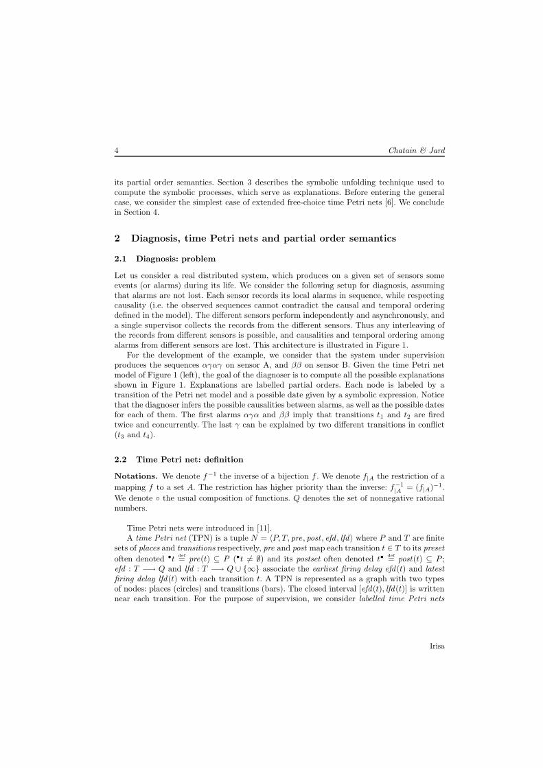
Time Petri nets were introduced in [11].A time Petri net (TPN) is a tuple N = 〈P, T, pre, post , efd , lfd〉 where P and T are finite

sets of places and transitions respectively, pre and post map each transition t ∈ T to its presetoften denoted •t

def= pre(t) ⊆ P (•t &= ∅) and its postset often denoted t•def= post(t) ⊆ P ;

efd : T −→ Q and lfd : T −→ Q ∪ {∞} associate the earliest firing delay efd(t) and latestfiring delay lfd(t) with each transition t. A TPN is represented as a graph with two typesof nodes: places (circles) and transitions (bars). The closed interval [efd(t), lfd(t)] is writtennear each transition. For the purpose of supervision, we consider labelled time Petri nets

Irisa

Time Supervision of Concurrent Systems 5

Diagnoser

System under super-vision

αΥαΥ

ββ

Sensor B

SensorA

P1 ●

P2 ●

P3 P4

t1

t3

t2t4

[0,∞[α

[2,2]γ

[1,2]β[0,0]

γ

t1

t2

t4

t1

t2

t3

e1(α)

e2(β)

e3(γ)e4(α)

e5(β)

e6(γ)

t1

t2

t4

t1

t2

t4

Explanations

P5

e1(α)

e2(β)

e3(γ)e4(α)

e5(β)

e7(γ)

Fig. 1. Model-based diagnosis of distributed systems using time Petri nets.

〈N,Λ,λ〉 where Λ is a set of event types (or alarms), and λ the typing of transitions (α,β, γin Figure 1).

A state of a time Petri net is given by a triple 〈M, dob, θ〉, where M ⊆ P is a markingdenoted with tokens (thick dots), θ ∈ Q is its date and dob : M −→ Q associates a date ofbirth dob(p) ≤ θ with each token (marked place) p ∈ M . A transition t ∈ T is enabled in thestate 〈M, dob, θ〉 if all of its input places are marked: •t ⊆ M . Its date of enabling doe(t) isthe date of birth of the youngest token in its input places: doe(t) def= maxp∈•t dob(p). All thetime Petri nets we consider in this article are safe, i.e. in each reachable state 〈M, dob, θ〉, ifa transition t is enabled in 〈M, dob, θ〉, then t• ∩ (M \ •t) = ∅.

A process of a TPN starts in an initial state 〈M0, dob0, θ0〉, which is given by the initialmarking M0 and the initial date θ0. Initially, all the tokens carry the date θ0 as date of birth:∀p ∈ M0 dob0(p) def= θ0.

The transition t can fire at date θ′ ≥ θ from state 〈M, dob, θ〉, if:

– t is enabled: •t ⊆ M ;– the minimum delay is reached: θ′ ≥ doe(t) + efd(t);– the enabled transitions do not overtake the maximum delays:

∀t′ ∈ T •t′ ⊆ M =⇒ θ′ ≤ doe(t′) + lfd(t′).

The firing of t at date θ′ leads to the state 〈(M \•t)∪t•, dob ′, θ′〉, where dob ′(p) def= dob(p)if p ∈ M \ •t and dob ′(p) def= θ′ if p ∈ t•.

PI n˚1740

6 Chatain & Jard

Finally we assume that time diverges: when infinitely many transitions fire, time neces-sarily diverges to infinity.

In the initial state of the net of Figure 1, p1 and p2 are marked and their date of birthis 0. t1 and t2 are enabled and their date of enabling is the initial date 0. t2 can fire in theinitial state at any time between 1 and 2. Choose time 1. After this firing p1 and p4 aremarked, t1 is the only enabled transition and it has already waited 1 time unit. t1 can fire atany time θ, provided it is greater than 1. Consider t1 fires at time 3. p3 and p4 are marked inthe new state, and transitions t3 and t4 are enabled, and their date of enabling is 3 becausethey have just been enabled by the firing of t1. To fire, t3 would have to wait 2 time units.But transition t4 cannot wait at all. So t4 will necessarily fire (at time 3), and t3 cannot fire.

Remark. The semantics of time Petri nets are often defined in a slightly different way: thestate of the net is given as a pair 〈M, I〉, where M is the marking, and I maps each enabledtransition t to the delay that has elapsed since it was enabled, that is θ − doe(t) with ournotations. It is more convenient for us to attach time information on the tokens of themarking than on the enabled transitions. We have chosen the date of birth of the tokensrather than their age, because we want to make the impact of the firing of transitions aslocal as possible. And the age of each token in the marking must be updated each timea transition t fires, whereas the date of birth has to be set only for the tokens that arecreated by t. Furthermore, usual semantics often deal with the delay between the firing oftwo consecutive transitions. In this paper we use the absolute firing date of the transitionsinstead. This fits better to our approach in which we are not interested in the total orderingof the events.

2.3 Partial order semantics

Processes. We will define the set X of (finite) processes of a safe time Petri net startingat date θ0 in the initial marking M0. These processes are those described in [1]. We definethem inductively and use a canonical coding like in [8]. The processes provide a partial orderrepresentation of the executions.

Each process will be a pair xdef= 〈E,Θ〉, where E is a set of events, and Θ : E −→ Q maps

each event to its firing date. Θ is sometimes represented as a set of pairs (e,Θ(e)). Eachevent e is a pair (•e, τ(e)) that codes an occurrence of the transition τ(e) in the process. •e

is a set of pairs bdef= (•b, place(b)) ∈ E × P . Such a pair is called a condition and refers to

the token that has been created by the event •b in the place place(b). We say that the evente

def= (•e, τ(e)) consumes the conditions in •e. Symmetrically the set {(e, p) | p ∈ τ(e)•} ofconditions that are created by e is denoted e•.

For all set B of conditions, we denote Place(B) def= {place(b) | b ∈ B}, and when therestriction of place to B is injective, we denote place−1

|B its inverse, and for all P ⊆ Place(B),

Place−1|B (P ) def= {place−1

|B (p) | b ∈ P}.The set of conditions that remain at the end of the process 〈E,Θ〉 (meaning that

they have been created by an event of E, and no event of E has consumed them) is

Irisa

Time Supervision of Concurrent Systems 7

↑(E) def=⋃

e∈E e• \⋃

e∈E•e (it does not depend on Θ). The state that is reached after

the process 〈E,Θ〉 is 〈Place(↑(E)), dob, maxe∈E Θ(e)〉, where for all p ∈ Place(↑(E)),dob(p) def= Θ(•b), with b

def= place−1|↑(E)(p).

We define inductively the set X of (finite) processes of a time Petri net starting at dateθ0 in the initial marking M0 as follows:

– 〈{⊥}, {(⊥, θ0)}〉 ∈ X , where ⊥ def= (∅, ε) represents the initial event. Notice that theinitial event does not actually represent the firing of a transition, which explains the useof the special value ε /∈ T . For the same reason, the set of conditions that are createdby ⊥ is defined in a special way: ⊥• def= {(⊥, p) | p ∈ M0}.

– For all process 〈E,Θ〉 ∈ X leading to state 〈M, dob, θ〉, if a transition t can fire atdate θ′ ≥ θ from state 〈M, dob, θ〉, then 〈E ∪ {e},Θ ∪ {(e, θ′)}〉 ∈ X , where the evente

def= (Place−1|↑(E)(

•t), t) represents this firing of t.

We define the relation → on the events as: e → e′ iff e• ∩ •e′ &= ∅. The reflexive tran-sitive closure →∗ of → is called the causality relation. For all event e, we denote4e5 def= {f ∈ E | f →∗ e}, and for all set E of events, 4E5 def=

⋃e∈E4e5. We also define

cnds(E) def=⋃

e∈E e• the set of conditions created by the events of E.Two events of a process that are not causally related are said to be concurrent.

Symbolic processes. We choose to group the processes that differ only by their firingdates to obtain what we call a symbolic process.

A symbolic process of a time Petri net is a pair 〈E, pred〉 with pred : (E −→ Q) −→ bool,such that for all mapping Θ : E −→ Q, if pred(Θ), then 〈E,Θ〉 ∈ X .

In practice, pred is described by linear inequalities. Examples of symbolic processes aregiven in Figure 1. The first explanation groups all the processes formally defined as 〈E,Θ〉where E contains the six following events, with the associated firing dates (the initial event⊥ is not represented):

1 = ({(⊥, P1)}, t1) Θ(1) ≥ Θ(⊥)2 = ({(⊥, P2)}, t2) 1 ≤ Θ(2) −Θ(⊥) ≤ 23 = ({(1, P3), (2, P4)}, t4) Θ(3) = max{Θ(1),Θ(2)}4 = ({(3, P1)}, t1) Θ(4) = Θ(3)5 = ({(3, P2)}, t2) Θ(5) = Θ(3) + 26 = ({(4, P3)}, t3) Θ(6) = Θ(4) + 2

2.4 Diagnosis: formal problem setting

Consider a net N modeling a system and an observation O of this system, which associatesa finite sequence of observed alarms (λs,1, . . . ,λs,ns) with each sensor s. The set of sensorsis denoted S. For each sensor s, Λs indicates which alarms the sensor observes.

To compute a diagnosis, we propose to build a net D(N, O) whose processes correspondto the processes of N which satisfy the observation O. The idea is to constrain the model by

PI n˚1740

8 Chatain & Jard

adding new places and transitions so that each transition of the model that sends an alarmto a sensor s is not allowed to fire until all the previous alarms sent to s have been observed.

To achieve this we create a place sλ for each alarm λ that may be sent to the sensors, plus one place s. For each transition t that sends an alarm λ to the sensor s, we add sλ

to the postset of t. After the ith alarm is sent to s, a new transition ts,i which models theobservation of this alarm by s, removes the token from sλ and creates a token in the place s,meaning that the alarm has been observed. s is added to the preset of each transition thatsends an alarm to s, so that it cannot fire before the previous alarm has been observed. Thetransitions ts,i are connected through places ps,i so that they must fire one after another.

Formally, for a net Ndef= 〈P, T, pre, post , efd , lfd〉 and an observation O from a set S of

sensors, we define a net D(N, O) def= 〈P ′, T ′,wpre ′, pre ′, post ′, efd ′, lfd ′〉. This net is almost atime Petri net: a weak preset wpre ′(t) ⊆ pre ′(t), denoted ◦t has been added for each transitiont ∈ T ′; only the date of birth of the tokens in the weak preset participate in the definitionof the date of weak enabling of t, which replaces the date of enabling in the semantics:dowe(t) def= maxp∈◦t dob(p). In the processes, for each event e, we denote ◦e

def= Place−1|•e(

◦τ(e)).Notice that the net may reach a degenerated state 〈M, dob, θ〉 where a weakly enabledtransition t has overtaken its maximum firing date (θ > dowe(t) + lfd(t)). In D(N, O) thissituation does not occur in the processes that generate explanations.

D(N, O) is defined as follows (where 6 denotes the disjoint union):

– P ′ def= P 6 {s | s ∈ S} 6 {sλ | s ∈ S ∧ λ ∈ Λs} 6 {ps,i | s ∈ S, i = 0, . . . , ns};– T ′ def= T 6 {ts,i | s ∈ S, i = 1, . . . , ns};– for all t ∈ T , wpre ′(t) def= pre(t), pre ′(t) def= wpre ′(t) 6 {s | λ(t) ∈ Λs},

post ′(t) def= post(t) 6 {sλ(t) | λ(t) ∈ Λs},efd ′(t) def= efd(t) and lfd ′(t) def= lfd(t);

– wpre ′(ts,i) = pre ′(ts,i)def= {ps,i−1, sλs,i}, post ′(ts,i)

def= {ps,i, s} andefd ′(ts,i) = lfd ′(ts,i)

def= 0.

Figure 2 shows the net of Figure 1 constrained by the observation αγαγ from sensor Aand ββ from sensor B.

We call diagnosis of observation O on net N any set of symbolic pro-cesses of D(N, O), which contain all the processes 〈E,Θ〉 of D(N, O) such that:{ps,ns | s ∈ S} 6 {sλ | s ∈ S ∧ λ ∈ Λs} ⊆ Place(↑(E)). Unless the model contains loops ofnon observable events, these processes can be described by a finite set of symbolic processes.These processes can be projected to keep only the conditions and events which correspondto places and transitions of the model. Then we obtain all the processes of N that are com-patible with the observation O, as shown in Figure 1. The construction of the explanations isbased on the unfolding of D(N, O). The notion of unfolding allows us to use a compact rep-resentation of the processes by sharing the common prefixes. The temporal framework leadsnaturally to consider the new notion of symbolic unfolding that we detail in the followingsection.

Irisa

Time Supervision of Concurrent Systems 9

P1 ●

P2 ●

P3 P4

t1

t3

t2

t4

[0,∞[α

[2,2]γ

[1,2]β[0,0]

γ

A● B

●A1

A2

A3

A4

Aα

Aγ

Bβ

B1

B2

P5

Fig. 2. Our example of TPN, constrained by the observation αγαγ from sensor A and ββ from sensor B.

3 Symbolic unfoldings of time Petri nets

Symbolic unfoldings have already been addressed in the context of high-level Petri nets [7].In this section we define the symbolic unfolding of time Petri nets, i.e. a quite compactstructure that contains all the possible processes and exhibits concurrency. Actually thetime Petri nets are extended with weak presets 1, as required by our diagnosis approach (seeSection 2.4).

For symbolic unfoldings of classical time Petri nets, consider that the weak preset ◦t ofany transition t ∈ T is equal to its preset •t.

3.1 Pre-processes

For the construction of symbolic unfoldings of time Petri nets, we need the notion of pre-process, that extends the notion of process.

For all process 〈E,Θ〉, and for all nonempty, causally closed set of events E ′ ⊆ E (⊥ ∈ E′

and 4E′5 = E′), 〈E′,Θ|E′〉 is called a pre-process. We often write 〈E ′,Θ〉 instead of 〈E′,Θ|E′〉for short. The definition of the state that is reached after a process is also used for pre-processes. We define the prefix relation ≤ on pre-processes as follows:

〈E,Θ〉 ≤ 〈E′,Θ′〉 iff E ⊆ E′ ∧ Θ = Θ′|E

1 We assume that the net never reaches a degenerated state 〈M, dob, θ〉 where a weakly enabledtransition t has overtaken its maximum firing date (θ > dowe(t) + lfd(t)).

PI n˚1740

10 Chatain & Jard

3.2 Symbolic unfoldings of extended free choice time Petri nets

An extended free choice time Petri net is a time Petri net such that:

∀t, t′ ∈ T •t ∩ •t′ &= ∅ =⇒ •t = •t′.

We define the symbolic unfolding U of an extended free choice time Petri net by collectingall the events that appear in its processes: U

def=⋃

〈E,Θ〉∈X E.This unfolding has two important properties in the case of extended free choice time

Petri nets:

Theorem 1. Let E ⊆ U be a nonempty finite set of events and Θ : E −→ Q associate afiring date with each event of E. 〈E,Θ〉 is a pre-process iff:

4E5 = E (E is causally closed)!e, e′ ∈ E e &= e′ ∧ •e ∩ •e′ &= ∅ (E is conflict free)∀e ∈ E \ {⊥} lpred(e,Θ) (all the events respect the firing delays)

where

lpred(e,Θ) def=

Θ(e) ≥ maxb∈•e Θ(•b) (t is strongly enabled when e fires)Θ(e) ≥ dowe(t) + efd(t) (the earliest firing delay is reached)∀t′ ∈ T •t′ = •t =⇒ Θ(e) ≤ dowe(t′) + lfd(t′)

(the latest firing delays are respected)

with tdef= τ(e) and

for all t′ ∈ T such that •t′ = •t, dowe(t′) def= maxb∈Place−1|•e

(◦t′) Θ(•b).

Theorem 2. For all edef= (B, t) ∈ cnds(U) × T ,

e ∈ U iff

Place(B) = •t!f, f ′ ∈ 4e5 f &= f ′ ∧ •f ∩ •f ′ &= ∅∃Θ : 4e5 −→ Q ∀f ∈ 4e5 \ {⊥} lpred(f,Θ)

The first theorem gives a way to extract processes from the unfolding, while the secondtheorem gives a direct construction of the unfolding: adding a new event e just requiressolving linear constraints on the Θ(f), f ∈ 4e5. This also happens with symbolic unfoldingsof high-level Petri nets introduced in [7].

We do not give proofs for the theorems 1 and 2 as they are particular cases of thetheorems 3 and 4: the symbolic unfolding of extended free choice time Petri nets as definedin this section is the same as the symbolic unfolding we obtain if we use the general definitionof the next section.

Irisa

Time Supervision of Concurrent Systems 11

3.3 Symbolic unfoldings of time Petri nets: general case

If we define the symbolic unfolding of a time Petri net in the general case as we have donefor extended free choice time Petri nets, none of the two previous theorems hold: extractinga process from the unfolding becomes complex (see [1]); and especially we do not knowany direct way to build the unfolding. It is also interesting to notice that the union of twopre-processes 〈E,Θ〉 and 〈E′,Θ′〉 is not necessarily a pre-process, even if Θ|E∩E′ = Θ′

|E∩E′

and E ∪ E′ is conflict free. In the example of Figure 1, we observe this if 〈E,Θ〉 is theprocess which contains a firing of t1 at time 0 and a firing of t2 at time 1, and 〈E ′,Θ′〉 is thepre-process that we obtain by removing the firing of t2 from the process made of t1 at time0, t2 at time 2 and t3 at time 2. These difficulties come from the fact that the condition thatallows us to extend a process x

def= 〈E,Θ〉 with a new event e concerns all the state reachedafter the process x, and however the conditions in •e refer only to the tokens in the inputplaces of τ(e).

From now on we assume that we know a partition of the set P of places of the net insets Pi ⊆ P of mutually exclusive places2; more precisely we demand that for all reachablemarking M , Pi ∩ M is a singleton. For all place p ∈ Pi, we denote p

def= Pi \ {p}. In theexample of Figure 1, we will use the partition {p1, p3, p5}, {p2, p4}.

Notion of partial state. A partial state of a time Petri net is a triple 〈L, dob, θ〉 withL ⊆ P , θ ∈ Q is a date and dob : L −→ Q associates a date of birth dob(p) ≤ θ with eachtoken (marked place) p ∈ L.

We define the relation 9 on partial states as follows:〈L, dob, θ〉 9 〈L′, dob ′, θ′〉 iff L ⊆ L′ ∧ dob = dob ′

|L ∧ θ ≤ θ′

Firing a transition from a partial state. Although the semantics of time Petri netsrequires to check time conditions for all the enabled transitions in the net, before firing atransition, there are cases when we know that a transition can fire at a given date θ′, evenif other transitions will fire before θ′ in other parts of the net. As an example consider thenet of Figure 1 starting at date 0 with the marking {p1, p2}. Although the semantics forbidsto fire t1 at date 10 before firing t2, we feel that nothing can prevent t1 from firing at date10, because only t1 can remove the token in place p1. By contrast, the firing of t3 highlydepends on the firing date of t2 because when t4 is enabled it fires immediately and disablest3. So if we want to fire t3 we have to check whether p2 or p4 is marked.

A partial state firing is a triple (S, t, θ′) where Sdef= 〈L, dobL, θL〉 is a partial state, t is a

transition such that •t ⊆ L, and θ′ ≥ θL is a date.2 If we do not know any such partition, a solution is to extend the structure of the net with one

complementary place for each place of the net and to add these new places in the preset (butnot in the weak preset) and in the postset of the transitions such that in any reachable markingeach place p ∈ P is marked iff its complementary place is not. This operation does not changethe behaviour of the time Petri net: since the weak presets do not change, the tokens in thecomplementary places do not participate in the definition of the date of enabling.

PI n˚1740

12 Chatain & Jard

The idea in partial state firings is that the partial state S gives enough information tobe sure that t can fire at date θ′.

It will be crucial in the following to know how to select partial state firings. Howeverseveral choices are possible. If we are given a predicate PSF on partial state firings, we canbuild extended processes by using only the extended processes that satisfy PSF . Then wewill try to map these extended processes into pre-processes. If PSF is valid, then all thepre-processes we obtain are correct.

Extended processes. Let PSF be a predicate on partial state firings.We will define a notion of extended process (parameterized by PSF ), which is close to

the notion of process, but the events are replaced by extended events which represent firingsfrom partial states and keep track of all the conditions corresponding to the partial state,not only those that are consumed by the transition: the other conditions will be treated ascontext of the event. This uses classical techniques of contextual nets or nets with read arcs(see [2,14]). It would also be possible to consume and rewrite the conditions in the contextof an event, but we feel that the notion of read arc or contextual is a good way to capturethe idea that we develop here.

For all extended event edef= (B, t), use the notations τ(e) def= t, •e

def= Place−1|B (•t),

◦edef= Place−1

|B (◦t), edef= B \ •e and e•

def= {(e, p) | p ∈ t•}. We define the relations → and ↗between extended events as:

– e → f iff e• ∩ (•f ∪ f) &= ∅ and– e ↗ f iff (e → f) ∨ (e ∩ •f &= ∅).

Like for processes, we define the set of conditions that remain at the end of the extendedprocess 〈E,Θ〉 as ↑(E) def=

⋃e∈E e• \

⋃e∈E

•e. But for extended processes we define not onlythe global state that is reached after 〈E,Θ〉, but a partial state RSΘ(B) associated witheach set of conditions B ⊆ ↑(E). The partial state associated with B does not depend on theset of events E provided

⋃b∈B4•b5 ⊆ E. It is defined as RSΘ(B) def= 〈Place(B), dobL, θL〉,

where dobL(p) def= Θ(•(place−1|B (p))) and θL

def= maxb∈B Θ(•b).We define the set XPSF of extended processes of a time Petri net starting at date θ0 in

the initial marking M0 as follows.

– Like for processes, 〈{⊥}, {(⊥, θ0)}〉 ∈ XPSF , where ⊥ def= (∅, ε) represents the initialevent. The set of conditions that are created by ⊥ is defined as: ⊥• def= {(⊥, p) | p ∈ M0}.

– For all extended process 〈E,Θ〉 ∈ XPSF , for all edef= (B, t) with B ⊆ ↑(E), and t ∈ T , for

all θ′ ≥ maxf∈E, f↗e Θ(f), if PSF (RSΘ(B), t, θ′) holds, then 〈E ∪ {e},Θ ∪ {(e, θ′)}〉 ∈XPSF .

Each extended event e can be mapped to the corresponding event

h(e) def=({

(h(f), p) | (f , p) ∈ •e}, τ(e)

).

Irisa

Time Supervision of Concurrent Systems 13

Corectness of PSF . We say that PSF is a valid predicate on partial state firings iff forall extended process 〈E,Θ〉 ∈ XPSF , 〈h(E),Θ ◦ h−1

|E 〉 is a pre-process (notice that h|E is

injective). In other terms there exists a process 〈E ′,Θ′〉 ∈ X such that 〈h(E),Θ ◦ h−1|E 〉 ≤

〈E′,Θ′〉.

Symbolic unfolding. As we did for extended free choice time Petri nets with events inSection 3.2, we define the symbolic unfolding UPSF of a time Petri net by collecting all theextended events that appear in its extended processes: UPSF

def=⋃

〈E,Θ〉∈XPSFE.

We have equivalents of the two theorems we had with symbolic unfoldings of extendedfree choice time Petri nets.

Theorem 3. Let E ⊆ UPSF be a nonempty finite set of extended events and Θ : E −→ Qassociate a firing date with each extended event of E. 〈E,Θ〉 is an extended process iff:

4E5 = E (E is causally closed)!e, e′ ∈ E e &= e′ ∧ •e ∩ •e′ &= ∅ (E is conflict free)!e0, e1, . . . , en ∈ E e0 ↗ e1 ↗ · · · ↗ en ↗ e0 (↗ is acyclic on E)∀e, e′ ∈ E e ↗ e′ =⇒ Θ(e) ≤ Θ(e′) (Θ is compatible with ↗)∀e ∈ E \ {⊥} PSF (RSΘ(•e ∪ e), τ(e),Θ(e)) (e corresponds to a partial state firing)

Proof. Let 〈E,Θ〉 ∈ XPSF be an extended process that satisfies the conditions in the curlybrace, let e

def= (B, t) with B ⊆ ↑(E) and t ∈ T and θ′ ≥ maxf∈E, f↗e Θ(f ) such thatPSF (RSΘ(B), t, θ′) holds. Then we will show that the extended process 〈E′,Θ′〉 def= 〈E ∪{e},Θ ∪ {(e, θ′)}〉 also satisfies the conditions in the curly brace. By construction E′ iscausally closed. Moreover for each condition b ∈ •e that is consumed by e, b ∈ ↑(E), whichimplies that b has not been consumed by any event of E. Thus for all f ∈ E, •e∩•f = ∅ and¬(e ↗ f). So E′ is conflict free and ↗ is acyclic on E′. Θ′ is compatible with ↗ because Θis compatible with ↗ and Θ′(e) = θ′ ≥ maxf∈E, f↗e Θ(f ).

Conversely let 〈E′,Θ′〉 satisfy the conditions in the curly brace. If E′ = {⊥}, then〈E′,Θ′〉 ∈ XPSF . Otherwise let e ∈ E′ be an extended event that has no succes-sor by ↗ in E′ (such an extended event exists since ↗ is acyclic on E′). 〈E,Θ〉 def=〈E′ \ {e},Θ′

|E′\{e}〉 satisfies the conditions in the curly brace. Assume that 〈E,Θ〉 ∈ XPSF .

As E is conflict free, •e ⊆ ↑(E). And as e has no successor by ↗ in E′, e ⊆ ↑(E).Furthermore Θ′(e) ≥ maxf∈E, f↗e Θ(f ) and PSF (RSΘ′(•e ∪ e), τ(e),Θ′(e)) holds. Thus〈E′,Θ′〉 = 〈E ∪ {e},Θ ∪ {(e,Θ′(e))}〉 ∈ XPSF .

Theorem 4. For all edef= (B, t) ∈ cnds(UPSF ) × T , e ∈ UPSF iff

!f , f ′ ∈ 4e5 f &= f ′ ∧ •f ∩ •f ′ &= ∅ (1)!e0, e1, . . . , en ∈ 4e5 e0 ↗ e1 ↗ · · · ↗ en ↗ e0 (2)

∃Θ : 4e5 −→ Q

{∀f , f ′ ∈ 4e5 f ↗ f ′ =⇒ Θ(f ) ≤ Θ(f ′)∀f ∈ 4e5 \ {⊥} PSF

(RSΘ(•f ∪ f), τ(f ),Θ(f)

) (3)

PI n˚1740

14 Chatain & Jard

Proof. Let e ∈ UPSF . There exists 〈E,Θ′〉 ∈ XPSF such that e ∈ E. 〈E,Θ′〉 satisfies theconditions in the curly brace of Theorem 3. As 4E5 ⊆ E, 4e5 also satisfies them. Then (1)and (2) hold. For (3) a possible Θ is Θ′

|+e,.

Conversely if edef= (B, t) satisfies (1), (2) and (3), consider a possible Θ for (3).

〈4e5 \ {e},Θ〉 satisfies the curly brace of Theorem 3. Then 〈4e5 \ {e},Θ〉 ∈ XPSF . More-over (1) implies that B ⊆ ↑(4e5 \ {e}). In addition Θ(e) ≥ maxf∈+e,, f↗e Θ(f ) andPSF (RSΘ(B), t,Θ(e)) holds. Thus 〈4e5,Θ〉 ∈ XPSF and therefore e ∈ UPSF .

Selecting partial state firings. The definition of extended processes is parameterized bya predicate PSF on partial state firings: each extended event must correspond to a partialfiring that satisfies PSF , the others are forbidden. A good choice for PSF takes three notionsinto account: completeness, redundancy and preservation of concurrency.

Completeness. A predicate PSF on partial state firings is complete if for all process〈E,Θ〉 ∈ X , there exists an extended process 〈E,Θ′〉 ∈ XPSF such that 〈h(E),Θ′ ◦ h−1

|E 〉 =〈E,Θ〉.

Redundancy. Given a predicate PSF on partial state firings and a process 〈E,Θ〉 ∈ X,there may exist several extended processes 〈E,Θ′〉 ∈ XPSF such that 〈h(E),Θ′ ◦ h−1

|E 〉 =〈E,Θ〉. This is called redundancy. In particular, if PSF contains two partial state firings(〈L, dob, θ〉, t, θ′) and (〈L′, dob ′, θ〉, t, θ′) where L′ " L and dob ′ = dob |L′ , then all the ex-tended processes involving (〈L, dob, θ〉, t, θ′) are redundant.

A trivial choice for PSF which does not preserve any concurrency. A trivial complete pred-icate PSF is the predicate that demands that the state S is a global state, and then checkthat t can fire at date θ′ from S. In addition, this choice gives little redundancy. But theextended events of the extended processes that we obtain in this case are totally ordered bycausality. In other words, these processes do not exhibit any concurrency at all. Actually weget what we call firing sequences in interleaving semantics.

A proposition for PSF. What we want is a complete predicate on partial state firings thatgenerates as little redundancy as possible and that exhibits as much concurrency as possible.

We first define a predicate PSF ′ on partial state firings as follows:PSF ′(〈L, dobL, θ〉, t, θ′) iff

– t is enabled: •t ⊆ L;– the minimum delay is reached: θ′ ≥ doe(t) + efd(t);– the transitions that may consume tokens of L are disabled or do not overtake the max-

imum delays:

∀t′ ∈ T •t′ ∩ L &= ∅ =⇒{

∃p ∈ •t′ p ∩ L &= ∅∨ θ′ ≤ max

p∈◦t′∩Ldob(p) + lfd(t′)

Irisa

Time Supervision of Concurrent Systems 15

Now we define PSF by eliminating some redundancy in PSF ′:PSF (〈L, dob, θ〉, t, θ′) iff PSF ′(〈L, dob, θ〉, t, θ′) and there exists no L′ " L such thatPSF ′(〈L′, dob |L′ , θ〉, t, θ′).

It is important that the constraints (see Theorems 3 and 4) can be solved automatically:with the definition of PSF we have proposed here, the quantifiers (∀ and ∃) on placesand transitions expand into disjunctions and conjunctions. The result is a disjunction ofconjunctions of linear inequalities on the Θ(e). When a “max” appears in an inequality, thisinequality can be rewritten into the desired form. These systems are shown near the eventsin Figure 3.

Theorem 5. PSF is a valid, complete predicate on partial state firings.

Proof. The proof of the validity is done in two parts:

1. For all 〈E,Θ〉 ∈ XPSF , denote 〈M, dob, θ〉 the global state reached after 〈E,Θ〉.〈h(E),Θ ◦ h−1

|E 〉 ∈ X iff

∀t ∈ T •t ⊆ M =⇒ θ ≤ dowe(t) + lfd(t). (1)

2. For all 〈E,Θ〉 ∈ XPSF , there exists 〈E′,Θ′〉 ∈ XPSF which satisfies (1) and such that〈E,Θ〉 ≤ 〈E′,Θ′〉.Consequently 〈h(E),Θ ◦ h−1

|E 〉 ≤ 〈h(E′),Θ′ ◦ h−1|E′〉 ∈ X .

Here are the proofs for these two points:

1. Let 〈E,Θ〉 ∈ XPSF and denote 〈M, dob, θ〉 the global state reached after 〈E,Θ〉.It follows from the definition of the processes that if 〈h(E),Θ◦h−1

|E 〉 ∈ X , then (1) holds.

Conversely, assume that 〈E,Θ〉 satisfies (1); choose e ∈ E such that Θ(e) = θ and !f ∈ Esuch that e ↗ f . Then denote 〈M ′, dob ′, θ′〉 the global state reached after 〈E \ {e},Θ〉and let t ∈ T such that •t ⊆ M ′. If •t∩•τ(e) = ∅, then dowe ′(t) = dowe(t) ≥ θ− lfd(t) ≥θ′ − lfd(t). Otherwise let L

def= •e ∪ e. As PSF (RSΘ(L), τ(e),Θ(e)) holds, then{

∃p ∈ •t p ∩ L &= ∅∨ θ ≤ max

p∈◦t∩Ldob ′(p) + lfd(t)

As •t ⊆ M ′, then !p ∈ •t such that p ∩ L &= ∅; thus θ ≤ maxp∈◦t∩L

dob ′(p) + lfd(t).

Hence dowe ′(t) = maxp∈◦t

dob ′(p) ≥ maxp∈◦t∩L

dob ′(p) ≥ θ − lfd(t) ≥ θ′ − lfd(t). As a result

〈E \ {e},Θ〉 ∈ XPSF and satisfies (1).Assume now that 〈E,Θ′〉 def= 〈h(E \ {e}),Θ ◦ h−1

|E 〉 ∈ X . It leads to 〈M ′, dob ′, θ′〉. As•τ(e) ⊆ M ′ and θ ≥ θ′ and θ ≥ dowe ′(τ(e)) + efd(τ(e)) and for all t ∈ T , •t ⊆ M ′ =⇒θ ≤ dowe ′(t) + lfd(t), then τ(e) can fire at date θ from 〈M ′, dob ′, θ′〉, which is coded bythe event (Place−1

|↑(E)(τ(e)), τ(e)) = h(e). Thus 〈h(E),Θ ◦ h−1|E 〉 ∈ X .

PI n˚1740

16 Chatain & Jard

2. Let 〈E,Θ〉 ∈ XPSF . If 〈E,Θ〉 satifies (1), then 〈E′,Θ′〉 def= 〈E,Θ〉 fits.Otherwise, choose t ∈ T such that •t ⊆ M ∧ θ > dowe(t) + lfd(t) and such thatt minimizes θt

def= dowe(t) + lfd(t). Let Fdef= {f ∈ E | Θ(f ) ≤ θt}. 〈F ,Θ|F 〉 ∈ XPSF .

Denote 〈M ′, dob ′, θ′〉 the global state reached after 〈F ,Θ|F 〉. PSF ′(〈M ′, dob ′, θ′〉, t, θt)holds. Thus there exists L ⊆ M ′ such that PSF (〈L, dob ′

|L, θ′〉, t, θt) holds. Let edef=

(Place−1|↑(F )

(L), t). We will show that 〈E ∪ {e},Θ ∪ {(e, θt)}〉 ∈ XPSF . Θ ∪ {(e, θt)} is

compatible with ↗: if an extended event f ∈ E is such that f ∩ •e &= ∅, then Θ(f ) ≤θt and if •f ∩ e &= ∅, then Θ(f) > θt. The strict inequality in the second case alsoguarantees that ↗ is acyclic on E ∪ {e}. As a result, we have built an extended process〈E ∪ {e},Θ ∪ {(e, θt)}〉 ∈ XPSF by adding the event to 〈E,Θ〉.Iterating this until 〈E,Θ〉 satisfies (1) terminates if we assume that time diverges: ateach step 〈F ,Θ|F 〉 satisfies (1), so 〈h(F ),Θ◦h−1

|F 〉 ∈ X ; moreover this process has strictlymore events at each step and the dates remain below θ, which does not increase.

This ends the proof of the validity of PSF . Now we have to prove that PSF is complete.Let 〈E,Θ〉 ∈ X leading to the global state 〈M, dob, θ〉, let t ∈ T be a transition that canfire at date θ′ ≥ θ from 〈M, dob, θ〉, and assume that there exists an extended process〈E,Θ′〉 ∈ XPSF such that 〈h(E),Θ′ ◦ h−1

|E 〉 = 〈E,Θ〉. PSF ′(〈M, dob, θ〉, t, θ′) holds. Thus

there exists L ⊆ M such that PSF (〈L, dob |L, θ〉, t, θ′) holds. Define edef= (Place−1

|↑E(L), t).

〈E ∪ {e},Θ′ ∪ {(e, θ′)}〉 ∈ XPSF and the event h(e) codes the firing of t at date θ′ after〈E,Θ〉.

3.4 Example of unfolding

We come back to our simple example of time Petri net given in Figure 1. Figure 3 shows aprefix of its symbolic unfolding. We have kept all the events concerned with the observations(this filtering is done by considering the time net D(N, O) defined in subsection 2.4). Tokeep the figure readable, we do not show in the unfolding the supplementary places andtransitions induced by the observations).

The explanations of Figure 1, given as symbolic processes, correspond to extended pro-cesses that appear in the prefix of unfolding of Figure 3. In this figure the rectangles representthe events, and the circles represent the conditions. An arrow from a condition b to an evente means that b ∈ •e. An arrow from an event e to a condition b means that b ∈ e•. A linewithout arrow between a condition b and an event e means that b ∈ e.

The constraint PSF (RSΘ(•e ∪ e), τ(e),Θ(e)) is represented near each event e of Figure 3.While extracting an extending process from this unfolding, we can solve the conjunction ofthe constraints appearing on the events of the extended process, plus the constraints thatensure that Θ is compatible with ↗. This gives all the possible values for the dates of theevents. For example, consider the extended process {e1, e2, e3, e4, e5, e6}. We obtain the

Irisa

Time Supervision of Concurrent Systems 17

following constraints:

0 ≤ Θ(e1) −Θ(⊥)1 ≤ Θ(e2) −Θ(⊥) ≤ 2Θ(e3) = max{Θ(e1), Theta(e2)}Θ(e3) −Θ(e1) ≤ 2 (t3 has not consumed

the token in p3 before t4 fires.)0 ≤ Θ(e4) −Θ(e3)1 ≤ Θ(e5) −Θ(e3) ≤ 2Θ(e6) −Θ(e4) = 2Θ(e6) −Θ(e3) ≤ 2 (t2 has not consumed

the token in p2 before t3 fires.)

∀e PSF (RSΘ(•e ∪ e), τ(e),Θ(e))

Θ(⊥) ≤ Θ(e1)Θ(⊥) ≤ Θ(e2)Θ(e1) ≤ Θ(e3)Θ(e2) ≤ Θ(e3)Θ(e3) ≤ Θ(e4)Θ(e3) ≤ Θ(e6)Θ(e4) ≤ Θ(e6)Θ(e3) ≤ Θ(e5)Θ(e6) ≤ Θ(e5)

∀e, e′ e ↗ e′ =⇒ Θ(e) ≤ Θ(e′).Notice that e6 ↗ e5.

These constraints can be simplified into:

Θ(⊥) ≤ Θ(e1)1 ≤ Θ(e2) −Θ(⊥) ≤ 2Θ(e3) = max{Θ(e1),Θ(e2)}Θ(e4) = Θ(e3)Θ(e6) = Θ(e4) + 2Θ(e5) = Θ(e3) + 2

The three maximal extended processes of Figure 3 share the prefix {e1, e2, e3, e4, e5}.The first extended process contains also e7. It corresponds to the second explanation ofFigure 1. The second extended process contains the prefix, plus e6 and the third containsthe prefix, plus e8. These two extended processes correspond to the same explanation: thefirst of Figure 1. This is what we have called redundancy. After solving the linear constraintswe see that the second occurrence of t1 must have occured immediately after t4 has firedand the second occurrence of t2 must have fired 2 time units later. Actually the extendedprocess with e6 and the one with e8 only differ by the fact that transition t3 has fired beforet2 in the first one, whereas t3 has fired after t2 in the second one. Because of transition t4,the firing of t2 has a strong influence on the firing of t3. This is the reason why there aretoo distinct cases in the unfolding.

PI n˚1740

18 Chatain & Jard

P1 P2

P3 P4

t1 t2

t4

e1 :0≤θ(e1)-θ(!!

e2 :1≤θ(e2)-θ(!!≤2

P1 P2

e3 :θ(e3)=max(θ(e1),θ(e2))

θ(e3)-θ(e1)≤2

P4

t2 e5 :1≤θ(e5)-θ(e3)≤2

P3

t1e4 :0≤θ(e4)-θ(e3)

t3 t4 t3

P1 P2 P5

e8 :θ(e8)-θ(e4)=2

θ(e8)≤max(θ(e4),θ(e5))

P5

e6 :θ(e6)-θ(e4)=2θ(e6)-θ(e3)≤2 e7 :

θ(e7)=max(θ(e4),θ(e5))θ(e7)-θ(e4)≤2

!

Fig. 3. A prefix of the symbolic unfolding of the time Petri net of Figure 1.

4 Conclusion

We have presented a possible approach to the supervision/diagnosis of timed systems, usingsafe time Petri nets. In such nets, time constraints are given by interval of nonnegative ra-tionals and are used to restrict the set of behaviours. The diagnosis problem is to recover thepossible behaviours from a set of observations. We consider that the observations are givenas a partial order (without any timing information) from the activity of several sensors. The

Irisa

Time Supervision of Concurrent Systems 19

goal of the supervisor is to select the possible timed behaviours of the model, which do notcontradict the observations: i.e. presents the same set of events labelled by the alarms and or-ders the events in the same direction that the sensors do. This goal is achevied by consideringa symbolic unfolding of time Petri nets, which is restricted by the observations. The result isa set of explanations, which explicit the causalities (both structural and temporal) betweenthe observations. At the same time, our algorithm infers the possible delays before the fir-ing of the transitions associated with them. Up to our knowledge, our symbolic unfoldingfor safe time Petri nets is original, and its application to compute symbolic explanations too.

A prototype implementation exists (a few thousands lines of Lisp code) and we plan touse it on real case studies. Another project is to define an algorithm to produce a completefinite prefix of the unfolding [9], which could be used for other applications than diagnosis(for which we do not need this notion since observations are finite sets).

At longer term, the notion of temporal diagnosis could be refined and revisited whenconsidering timed distributed systems, in which alarms could bring a time information.

References

1. Tuomas Aura and Johan Lilius. Time processes for time Petri nets. In ICATPN, pages 136–155,1997.

2. Paolo Baldan, Andrea Corradini, and Ugo Montanari. Contextual petri nets, asymmetric eventstructures, and processes. Inf. Comput., 171(1):1–49, 2001.

3. A. Benveniste, E. Fabre, C. Jard, and S. Haar. Diagnosis of asynchronous discrete event systems,a net unfolding approach. IEEE Transactions on Automatic Control, 48(5):714–727, May 2003.

4. Bernard Berthomieu and Michel Diaz. Modeling and verification of time dependent systemsusing time Petri nets. IEEE Trans. Software Eng., 17(3):259–273, 1991.

5. Bernard Berthomieu and Francois Vernadat. State class constructions for branching analysisof time Petri nets. In TACAS, pages 442–457, 2003.

6. Eike Best. Structure theory of Petri nets: the free choice hiatus. In Proceedings of an AdvancedCourse on Petri Nets: Central Models and Their Properties, Advances in Petri Nets 1986-PartI, pages 168–205, London, UK, 1987. Springer-Verlag.

7. Thomas Chatain and Claude Jard. Symbolic diagnosis of partially observable concurrent sys-tems. In FORTE, pages 326–342, 2004.

8. Joost Engelfriet. Branching processes of Petri nets. Acta Inf., 28(6):575–591, 1991.9. Javier Esparza, Stefan Romer, and Walter Vogler. An improvement of McMillan’s unfolding

algorithm. In TACAS, pages 87–106, 1996.10. Hans Fleischhack and Christian Stehno. Computing a finite prefix of a time Petri net. In

ICATPN, pages 163–181, 2002.11. P.M. Merlin and D.J. Farber. Recoverability of communication protocols – implications of a

theorical study. IEEE Transactions on Communications, 24, 1976.12. B. Pradin-Chezalviel, R. Valette, and L.A. Kunzle. Scenario duration characterization of t-

timed Petri nets using linear logic. In IEEE PNPM, pages 208–217, 1999.13. Alexei Semenov and Alexandre Yakovlev. Verification of asynchronous circuits using time Petri

net unfolding. In DAC’96: Proceedings of the 33rd annual conference on Design automation,pages 59–62, New York, NY, USA, 1996. ACM Press.

PI n˚1740

20 Chatain & Jard

14. Walter Vogler. Partial order semantics and read arcs. In MFCS, pages 508–517, 1997.

Irisa