i n s t i t u t d e s t a t i s t i q u e b i o s t a t i ... reddot/stat/documents... ·...
TRANSCRIPT

I N S T I T U T D E S T A T I S T I Q U E
B I O S T A T I S T I Q U E E T
S C I E N C E S A C T U A R I E L L E S
( I S B A )
UNIVERSITÉ CATHOLIQUE DE LOUVAIN
KLEIN, N., DENUIT, M., LANG, S. and T. KNEIB
D I S C U S S I O N
P A P E R
2013/45
Nonlife Ratemaking and Risk Management with Bayesian Additive Models for Location, Scale and Shape

Nonlife Ratemaking and Risk Management with
Bayesian Additive Models for Location, Scale and
Shape
Nadja Klein
University of Gottingen
Michel Denuit
Universite Catholique de Louvain
Stefan Lang
University of Innsbruck
Thomas Kneib
University of Gottingen
Abstract
Generalized additive models for location, scale and shape define a flexible, semi-
parametric class of regression models for analyzing insurance data in which the expo-
nential family assumption for the response is relaxed. This approach allows the actuary
to include risk factors not only in the mean but also in other parameters governing the
claiming behavior, like the degree of residual heterogeneity or the no-claim probability.
In this broader setting, the Negative Binomial regression with cell-specific heterogene-
ity and the zero-inflated Poisson regression with cell-specific additional probability
mass at zero are applied to model claim frequencies. Models for claim severities that
can be applied either per claim or aggregated per year are also presented. Bayesian
inference is based on efficient Markov chain Monte Carlo simulation techniques and
allows for the simultaneous estimation of possible nonlinear effects, spatial variations
and interactions between risk factors within the data set. To illustrate the relevance of
this approach, a detailed case study is proposed based on the Belgian motor insurance
portfolio studied in Denuit and Lang (2004).
Key words: overdispersed count data; mixed Poisson regression; zero-inflated Poisson;
Negative Binomial; zero-adjusted models; MCMC; probabilistic forecasts.
1

1 Introduction
Calculations of motor insurance premiums are based on detailed statistical analyses
of large data bases maintained by insurance companies, recording individual claim
experience. The actuarial evaluation relies on a statistical model incorporating all
the available information about the risk. Premiums then often vary by the territory
in which the vehicle is garaged, the use of the vehicle (driving to and from work
or business use) and individual characteristics (such as age, gender, occupation and
marital status of the main driver of the vehicle, for instance). If the policyholders
misrepresent any of these classification variables in their declaration, they are subject
to loss of coverage when they are involved in a claim. There is thus a strong incentive
for accurate reporting of risk characteristics making insurance data reliable.
It is now common practice to achieve a priori risk classification with the help of Gen-
eralized Linear Models (GLMs), see, e.g., Denuit et al. (2007) for an introduction in
relation with motor insurance. They are so called because they generalize the clas-
sical linear model based on the Normal distribution to similar regression models for
Poisson, Binomial, Gamma or Inverse-Gaussian responses, for instance. The main
drawback of GLMs is that covariate effects are modeled in the form of a linear pre-
dictor. This is not a problem for categorical explanatory variables coded by means of
binary variables, but a strong restriction for continuous explanatory variables which
may have a nonlinear effect on the score. It has been common practice in insurance
companies to model possibly nonlinear effects by means of polynomials. However, it
is now well documented that low-degree polynomials are often not flexible enough to
capture the variability in the data and that increasing their degree produces unstable
estimates, especially for extreme values of the covariates. Although banding results in
a loss of information, a model employing a banded version of a continuous covariate
is sometimes considered more practical than one which employs the (untransformed)
continuous variable. However, there is no general rule to determine the optimal choice
of cutoffs so that banding may bias risk evaluation.
Among continuous covariates, geographic area plays a particular role. It can either be
seen as a function of two coordinates if exact locations are available or a function of
an administrative areal variable if spatial information is aggregated for confidentiality
2

reasons. In any case, actuaries wish to estimate the spatial variation in risk premium
and to price accordingly. Spatial zip code methods for insurance rating attempt to
extract information which is in addition to that contained in standard factors (like age
or gender for instance). With the regression models discussed in the present paper,
the effect of continuous and spatial covariates is modeled on the score scale by means
of smooth, unspecified functions estimated from the data.
Generalized additive models (GAMs) as developed in Hastie and Tibshirani (1990)
and popularized by Wood (2006) provide a convenient framework to overcome the
linearity assumptions inherent to GLMs when smooth effects of continuous covariates
need to be included in an additive predictor. Inference can be realized by cross
validation as in Wood (2004), by mixed model representations as in Ruppert et al.
(2003), Fahrmeir et al. (2004) and Wood (2008) or by Markov chain Monte Carlo
(MCMC) simulations as in Brezger and Lang (2006), Julion and Lambert (2007) and
Lang et al. (2013).
The framework of generalized additive models for location, scale and shape
(GAMLSS) introduced by Rigby and Stasinopoulos (2005) allows to extend GAMs
to more complex response distributions where not only the expectation but multiple
parameters are related to structured additive predictors with the help of suitable link
functions. Structured additive regression relies on a unified representation of different
model terms like parametric linear effects, smooth nonlinear effects of continuous co-
variates, interaction terms based on varying coefficients and spatial effects (Fahrmeir
et al., 2013, Brezger and Lang, 2006). In particular, zero-inflated, skewed and zero-
adjusted distributions can be embedded in this framework as special cases where
all occurring parameters are related to regression predictors and may depend on a
complex covariate structure. All these model terms rely on a unifying representation
based on non-standard basis function specifications in combination with quadratic
penalties in a frequentist formulation or Gaussian priors in a Bayesian approach.
In this broader setting, the Poisson assumption for claim frequencies made in De-
nuit and Lang (2004) is replaced with a mixed Poisson one, with Gamma distributed
random effect (yielding the Negative Binomial distribution with cell-specific hetero-
geneity) or Bernoulli distributed random effect (yielding the zero-inflated Poisson
distribution with cell-specific additional probability mass at zero).
3

In addition to claim frequencies, we also consider regression models for claim sever-
ities. Much attention has been paid in the actuarial literature to find suitable dis-
tributions to model claim sizes; see for example Klugman et al. (2004). Whereas
Denuit and Lang (2004) studied claim frequencies and claim severities separately, we
consider in this paper the so-called zero-adjusted models that allow to account for
zeros in the analysis of the amount of loss directly without resorting to models for
claim frequencies. Zero-adjusted distributions combine a continuous distribution on
the positive real line and a point mass at zero, such that the probabilities for a claim
and quantiles of the claim size distribution can be estimated in one model. Zero-
adjusted models are in the line of Jørgensen and Paes de Souza (1994) and Smyth
and Jørgensen (2002) where the zero claims are included using the Tweedie distribu-
tion. However, this model has the disadvantage that the probability at zero cannot
depend on covariates whereas here, this key actuarial indicator is allowed to vary
according to risk characteristics.
To select an appropriate response distribution and to specify several predictors that
correspond for instance to variances, skewness or overdispersion of the distribution,
we rely mainly on the deviance information criterion (DIC) of Spiegelhalter et al.
(2002) whose performance in Bayesian count data regression within the framework of
GAMLSS has been tested in Klein et al. (2013a). The choice of the distribution will
be supported by normalized quantile residuals (Dunn and Smyth, 1996) and proper
scoring rules (Gneiting and Raftery, 2007).
We highlight the advantages of complex Bayesian count data, skewed and zero-
adjusted regression models for insurance claims data with a detailed analysis of a
Belgian data set with more than 160,000 policies. Specifically,
• we consider the Poisson, zero-inflated Poisson and Negative Binomial regression
models for claim frequencies, where suitable predictors are specified for the
expected number of claims as well as for the probability of the structural zeros
in zero-inflated Poisson and for the scale parameter of the Negative Binomial
distribution.
• for claim severities, we extend the continuous models to zero-adjusted versions
of the Gamma, Inverse-Gaussian and LogNormal distributions, we estimate the
corresponding location and scale or shape parameters as well as the probability
4

of a claim in terms of relevant covariates in an additive fashion.
• inference in all model formulations is based on iteratively weighted least squares
approximations to the full conditionals in Markov chain Monte Carlo (MCMC)
simulation techniques as suggested in Gamerman (1997) or Brezger and Lang
(2006) and extended to the general framework of GAMLSS by Klein et al.
(2013b).
• we benefit from a numerically efficient implementation in the free open software
BayesX also available via the R add-on package R2BayesX.
• compared to frequentist GAMLSS approaches, the approach adopted here di-
rectly includes the choice of smoothing parameters in the estimation run and
provides valid confidence intervals which are difficult to obtain from asymptotic
maximum likelihood theory.
Our approach to zero-inflated, skewed and zero-adjusted models has therefore the
full flexibility in the parametric distribution assumption. The structured additive
modeling of all parameters allows to focus on specific aspects of the data that go
beyond the mean. In particular,
• the separate modeling of the probability mass at zero as a function of the
observable characteristics allows for an accurate analysis of this key actuarial
indicator.
• cell-specific residual heterogeneity in the Negative Binomial model allows for
more accurate risk predictions when deriving the predictive distributions of
future claims.
• zero-augmented models for the annual claim amounts are in accordance with
the individual model of risk theory so that the actuarial analysis benefits from
the numerous tools developed in that setting.
The claim frequencies models considered in the present paper have already been ap-
plied to insurance data. See, e.g., Yip and Yau (2005) or Boucher et al. (2006). How-
ever, previous applications of Negative Binomial or zero-inflated Poisson regression
models to insurance data only allowed for linear effects of the covariates or applied
5

preliminary banding techniques to transform continuous covariates into categorical
ones. Zero-adjusted Gamma and Inverse-Gaussian models have been proposed by
Heller et al. (2006), Bortoluzzo et al. (2011) and Resti et al. (2013) but their analy-
sis only allowed for linear effects of the covariates, too. See also Heller et al. (2007)
for a related model extending the Tweedie construction beyond the Poisson-Gamma
setup. The present paper innovates in that nonlinear effects are allowed using the
efficient inference techniques developed by Klein et al. (2013a). The effect of contin-
uous covariates on the score are quantified by means of unknown smooth functions
that do not need to be specified a priori under parametric form but are estimated
directly from the data.
Let us now briefly present the data used to illustrate the techniques described in this
paper. The data set is the one analyzed in Denuit and Lang (2004) by means of
Poisson and LogNormal regression techniques. It relates to a Belgian motor third-
party liability insurance portfolio observed during the year 1997, comprising more
than 160,000 policies. The following information is available on an individual basis.
As far as policyholders’ characteristics are concerned, we know gender, age, place of
residence and use of the car. Concerning the insured vehicle, we have its ancientness,
the type of fuel, its power and whether the vehicle belongs to a fleet. About the
contract, we know the type of coverage (compulsory motor third party liability only,
or motor third party liability together with some optional coverages) and the level
occupied in the former Belgian bonus-malus scale. In addition to these covariates,
the number of claims filed by each policyholder during 1997, the exposure-to-risk
from which these claims originated, as well as the resulting total claim amount are
given. See Table 1 for a list of available explanatory variables with some descriptive
statistics.
Notice that the -1/+1 coding has been used for the binary covariates in Table 1
whereas actuaries usually resort to a 0/1 coding, with 0 for the most populated class
taken as reference (see, e.g., Denuit and Lang, 2004). This is because the -1/1 coding
often has a positive mixing behavior in MCMC. Of course, the actuary can easily
revert to the standard 0/1 coding, if needed, by an appropriate linear transformation
of the regression parameters. The extent of coverage has been coded in a similar way
6

Continuous covariates
variable description mean std dev. min/max
ageph age of policyholder 47 14.83 18/78
agec age of vehicle 7.35 4.12 0/30
power engine power 56.01 19.02 10/243
Binary covariates
variable description levels proportions in %
fuel fuel oils gas=1/diesel=-1 69.1/30.9
use use of vehicle work=1/private=-1 4.8/95.2
fleet belongings to a fleet yes=1/no=-1 3.2/96.8
sex gender of policyholder male=1/female=-1 73.5/26.5
Categorical covariates
variable description levels proportions in %
coverage guarantees subscribed TPL only (1) 58.2
TPL+limited material 28.3
damage and theft (2)
TPL+comprehensive damage (3) 13.6
bm bonus-malus level 0,. . . ,22
district spatial information 1,. . . ,589
Table 1: Covariates available in the car insurance data set.
7

by means of two auxiliary covariates cov1 and cov2 defined as follows:
cov1 = I[coverage = 1]− I[coverage = 3]
cov2 = I[coverage = 2]− I[coverage = 3]
where I[·] denotes the indicator function.
Even if it is common to include the gender of the main driver in the actuarial ratemak-
ing, some states have banned the commercial use of this rating factor (as in EU mem-
ber countries, for instance). Here, we assume that we deal with the technical price
list and we do not discuss the various adaptations made to produce the commercial
price list.
The remaining sections are organized as follows: In Section 2 we introduce the speci-
fication of Bayesian models for analyses of claim frequencies as well as severities. We
describe the underlying inference and we give guidelines for model choice. Sections
3 and 4 deal with claim frequency and claim severity models, respectively. The ap-
plicability of the proposed models is demonstrated on the Belgian data set presented
before. The analysis we conduct shows major improvements compared to existing
approaches and reveal new features of insurance data. Conclusions are given in the
last Section 5.
2 Regression Models
2.1 Generalized additive models for location scale and shape
(GAMLSS)
Suppose we have observations (yi,xi), i = 1, 2, . . . , n on a response variable Y and a
vector of covariates x. Here, Y may be either the claim size or the claim frequency.
The vector x is split up into a subset of continuous covariates, another subset of
categorical covariates, and geographical information. We assume that there are p
continuous covariates x1, . . . , xp, spatial region s, and that the remaining categorical
explanatory variables are coded by means of a vector z0 of covariates.
GAMLSS require a parametric distribution assumption for the response variable,
involving several parameters represented as functions of explanatory variables. In
8

GAMLSS the exponential family distribution assumption for the response Y is relaxed
so that the actuarial analysis is no more restricted to the distributions used in the
classical GLM setting. The systematic part of the model is expanded compared to
GLMs to allow modeling not only the mean (or location) but other parameters of the
distribution of the response as linear and/or nonlinear parametric and/or additive
non-parametric functions of explanatory variables.
More precisely, the model is built as follows: The form of the distribution assumed for
the response variable can be very general. The only restriction is that the individual
contribution to the log-likelihood and its first two derivatives with respect to each
of the parameters must be computable. Known monotonic link functions relate the
distribution parameters to explanatory variables. Specifically, distribution parameters
ϑ1, ϑ2, . . . are decomposed into hk(ϑk) = ηk for some known link function hk where
the score ηk is assumed to be of a semi-parametric additive form
ηk = z′0β0k +
p∑j=1
fkj(xj) + fk,spat(s)
where the functions fkj express the effect of continuous covariates on the score scale,
fk,spat accounts for spatial variations in the risk distribution, z′0β0k contains paramet-
ric, linear effects of covariates.
All the distribution parameters can be decomposed on the score scale as linear, non-
linear parametric, non-parametric (smooth) functions or spatial variations of the ex-
planatory variables. The parameters are estimated within the GAMLSS framework
by maximizing a penalized likelihood function. More details on how the penalized log
likelihood is maximized are given in Rigby and Stasinopoulos (2005). The available
distributions include all those commonly used in actuarial analyses. See Table 1 in
Stasinopoulos and Rigby (2007) for an exhaustive list.
2.2 Bayesian structured additive regression
Hereafter, we give a brief overview of the statistical concepts used in the GAMLSS
model terms. A more tutorial style introduction is given in Denuit and Lang (2004)
and in the textbook by Fahrmeir et al. (2013). In structured additive regression
each vector f containing the evaluations of a function f at the observed covariates
is approximated in terms of appropriate basis functions which allows the unified
9

representation
f = Zβ
where Z is a design matrix arising from evaluations of the basis functions and β is
the vector of regression coefficients.
Each predictor from the previous section can therefore be expressed in terms of
η = Z0β0 +Z1β1 + . . .+Zpβp +Zspatβspat
where for simplicity we drop the parameter name.
In a Bayesian framework a standard smoothness prior is a (possibly improper) Gaus-
sian prior of the form
p(β|τ 2) ∝(
1
τ 2
)rank(K)/2
exp
(− 1
2τ 2β′Kβ
)· I[Aβ = 0] (1)
where β may be any of the vectors β0,β1, . . . ,βp,βspat. The key components of
the prior are the penalty matrix K, the variance parameter τ 2 and the constraint
Aβ = 0.
The structure of the penalty or prior precision matrix K depends on the covariate
type and on prior assumptions about smoothness of f , see below. Usually, the penalty
matrix in our examples is rank deficient resulting in a partially improper prior. The
amount of smoothness is governed by the variance parameter τ 2: The smaller the
variance, the smoother the function estimates and the other way around. A conjugate
inverse Gamma prior is employed for τ 2 with small values for the hyperparameters
resulting in an uninformative prior on the log scale.
For instance, for modeling the nonlinear effect f(ageph) we apply Bayesian
P(enalized)-splines as proposed in Lang and Brezger (2004). P-splines assume that
the unknown functions can be approximated by a polynomial spline which can be
written in terms of a linear combination of B-spline basis functions. Hence, the
columns of the design matrix Z are given by the B-spline basis functions evaluated
at the observations. Lang and Brezger (2004) propose to use first or second order
random walks as smoothness priors for the regression coefficients, i.e.
βl = βl−1 + ul, or βl = 2βl−1 − βl−2 + ul, (2)
with Gaussian centered errors ul with common variance τ 2j and diffuse priors p(β1) ∝
const, or p(β1) and p(β2) ∝ const, for initial values. This prior is of the form (1) with
10

penalty matrix given by K = D′D, where D is a first or second order difference
matrix.
A common way to deal with the spatial covariate distr is to define a neighborhood
structure ∂s on the set {1, . . . , 589} of districts in Belgium and to assume that neigh-
boring regions are similar. In our case neighborhoods are simply given by common
borders. The design matrix is an indicator matrix connecting individual observations
with corresponding regions, i.e. the entry (i, s) of the matrix Z is one if observation
i belongs to region s and zero otherwise. To implement spatial smoothness, K is
chosen as an adjacency matrix indicating which regions are neighbors of each others,
see Rue and Held (2005) for details. The simplest smoothness prior is called Markov
random field. In this case, given βr, r 6= s and hyperparameter τ 2, βs is Normally dis-
tributed with mean∑
r∈∂s1
Nsβr and variance τ2
Ns, where Ns is the number of neighbors
of region s. In consequence, the conditional mean of βs given all other coefficients is
the average of the neighborhood regions. Further background about Markov random
fields can be found in Fahrmeir et al. (2013).
Especially in the application on claim sizes, it is useful to split up the effect fspat
into a spatially structured (smooth) effect fstr and a spatially unstructured effect
funstr, i.e. fspat = fstr + funstr. The unstructured part is modeled by independent and
identically distributed Gaussian random effects, i.e. Z is again an indicator matrix
as in the Markov random field and β is multivariate Normal with zero mean and
diagonal covariance matrix.
The type of modeling discussed so far can be embedded in a computationally very
powerful multilevel version of structured additive regression models where regression
coefficients may themselves depend on covariates and can be modeled by a structured
additive predictor. We refer the reader to Lang et al. (2013) for details. Bayesian
inference is based on highly efficient Markov chain simulation based on iteratively
weighted least squares proposals as suggested by Gamerman (1997) or Brezger and
Lang (2006) and for the models at hand in a recent paper by Klein et al. (2013b).
2.3 Model choice and predictive ability
Since we are dealing with many (possibly nonlinear) covariate effects and usually
several additive predictors, adequate model choice plays a crucial role when apply-
11

ing GAMLSS. Unfortunately, many diagnostic tools in Bayesian inference based on
MCMC are only useful for restricted classes of simple models with just a few pa-
rameters. Klein et al. (2013b) proposed a practical procedure for model selection in
Bayesian GAMLSS to find a suitable response distribution as well as parsimonious
specifications for all model predictors. We mainly follow their proposals since they
do not only focus on improving the fit to the data but also the quality of predictions
for new observations.
A first measure for the model fit that takes the estimated model complexity into
account is the deviance information criterion (DIC) proposed by Spiegelhalter et
al. (2002) that has become quite popular in Bayesian statistics as it can easily
be computed from the MCMC output. Let ϑ denote the vector of model param-
eters. If ϑ(1), . . . ,ϑ(T ) is an MCMC sample from the posterior distribution of model
parameters, then the DIC is based on the following two quantities: The deviance
D(ϑ) = −2 log(p(y|ϑ)) of the model that reflects the fit of the data and model com-
plexity through the effective number of parameters in the model pD. As derived by
Spiegelhalter et al. (2002), the latter is given by the difference of the posterior mean
of the deviance and the deviance of the posterior means, i.e. pD = D(ϑ) − D(ϑ),
where
D(ϑ) =1
T
T∑t=1
D(ϑ(t))
and ϑ =1
T
T∑t=1
ϑ(t).
The DIC is then defined as
DIC = D(ϑ) + 2pD = 2D(ϑ)−D(ϑ)
indicating a close relationship to the frequentist Akaike information criterion that
provides a similar compromise between fidelity to the data and model complexity.
A rough rule of thumb says that DIC differences of 10 and more between two com-
peting models indicate the model with the lower DIC to be superior. For fixed dis-
tributional assumptions for the response, we use the DIC for variable selection in all
predictors, as already described in the previous section. If for one distribution with
different parameter specifications several models have similar DIC with differences
smaller than 10, we usually decide for the sparser model in the sense that additional
non-significant effects are excluded from the predictors. Our variable selection typi-
cally starts with the examination of the location parameter of the distributions. After
12

having a reasonable predictor for this main parameter, we continue in determining
the remaining predictors by a stepwise search. Note that the performance of the DIC
in count data models has been evaluated in the supplement of Klein et al. (2013a)
and rated to provide valid guidance.
For discriminating between competing response distributions, we rely on normalized
quantile residuals and proper scoring rules. Stasinopoulos et al. (2008) suggested
normalized quantile residuals as a graphical device. For continuous response data,
the quantile residual relies on ui = Fi(yi|ϑ), where Fi is the cumulative distribution
function estimated for the ith individual, ϑ contains all estimated model parameters
and yi is the corresponding observation. If the estimated Fi is close to the true dis-
tribution of yi then ui approximately follows a uniform distribution. To use standard
quantile-quantile plots for the graphical investigation of the model fit, the residual
is finally defined as ri = Φ−1(ui) where Φ−1 is the inverse cumulative distribution
function of the standard Normal distribution. Hence, ri is approximately standard
Normal if the estimated model is close to the true one. For discrete response dis-
tributions, the definition has to be slightly extended and ui is defined as a random
number from the uniform distribution on the interval [Fi(yi − 1|ϑ), Fi(yi|ϑ)]. In any
case, the model fit can be evaluated by means of usual quantile-quantile plots: The
closer the residuals to the bisecting line, the better the fit to the data.
Gneiting and Raftery (2007) propose proper scoring rules as summary measures for
the evaluation of probabilistic forecasts based on the predictive distribution and the
observed realizations. In our analysis, we apply a selection of these scores that have
been assigned to the general framework of regression in GAMLSS by Klein et al.
(2013b). There are several candidates for the score function S, depending on whether
the response variable is discrete, continuous or mixed discrete-continuous. In all three
cases, we use the logarithmic, quadratic and spherical score which are all proper
scoring rules meaning that if Gi is the true distribution of the response yi then
S(Gi, Gi) ≥ S(Gi, Fi) holds for all Fi 6= Gi. We refer the reader to Gneiting and
Raftery (2007) for further details on these scores. In practice, the predictive distribu-
tions Fi for observations yi are obtained by ten-fold cross validation, that is, 10% of
the data set is left out and the parameters of the distributions are predicted based on
the estimations of the remaining 90%. The scores are then the sum of individual con-
13

tributions, where higher scores deliver better probabilistic forecasts when comparing
different models.
Since the total score is only a summary measure for the complete predictive distri-
bution, it does not allow to assess which parts of the true response distribution are
reflected well in the model and which aspects differ from the truth. For example,
there may be a distribution that fits the central part of the data well but fails to fit
the tails. In terms of a summarized score, it may then be difficult to distinguish this
behavior from another candidate distribution that differs from the true distribution
slightly over the whole domain. In such a case, it can be helpful to follow Gneiting
and Ranjan (2011) who suggest a quantile decomposition of the quantile score given
by
−2
∫ 1
0
(I[yi ≤ F−1
i (α)]− α
) (F−1i (α)− yi
)dα.
In this way, the performance of the distributions can be compared with respect to the
ability to fit specific quantiles of the true distribution. We apply this score later on to
compare distributions for analyzing the claim sizes and to determine claim sizes that
cause the largest deteriorations in the score. The whole integral over the quantile
decomposition leads to the continuous ranked probability score (CRPS) which is also
a proper scoring rule directly formulated in terms of the cumulative distribution
functions while the logarithmic, quadratic and spherical scores are computed from
the densities.
3 Modelling Claim Frequencies: Count Data Re-
gression
3.1 Negative Binomial regression with cell-specific hetero-
geneity
Insurance data often exhibits overdispersion because several important risk attitudes
cannot be observed (swiftness of reflexes, aggressiveness behind the wheel, consump-
tion of drugs, etc.). This can be modeled by the inclusion of a random heterogeneity
factor. Specifically, given Θi = θ, the number of claims Ni reported by policy-
holder i conforms to the Poisson distribution with mean µiθ. Here, we consider that
14

Θ1,Θ2,Θ3, . . . are independent and Gamma distributed random variables, with unit
mean and scale parameter δi depending on covariates (so that the heterogeneity may
be specific to risk classes). Therefore we obtain a Negative Binomial (NB) distribution
for Ni, that is,
Pr[Ni = k] =Γ(k + δi)
Γ(k + 1)Γ(δi)
( µiδi + µi
)k( δiδi + µi
)δi, k = 0, 1, 2, . . . (3)
where Γ(a) =∫∞
0exp(−t)ta−1dt for a > 0.
To compare with the results obtained by Denuit and Lang (2004), we also consider
the Poisson regression model for claim counts where Ni obeys the Poisson distribution
with mean λi. Both µ and λ are expressed in terms of frequency scores ηfreq using
log link, i.e. λfreq = exp(ηλfreq) and µfreq = exp(ηµfreq). In both cases, we end up with a
frequency score of the form
fµ1 (ageph) + sex fµ2 (ageph) + fµ3 (agec) + fµ4 (bm) + fµ5 (power) + fµspat(distr) + (zµ)′ β.
where µ is replaced by λ to obtain the frequency score of the Poisson model. Here,
z contains the linear effects fuel , coverage and fleet , an intercept and the logarithm
of the contract periods in days. The other categorical covariates do not significantly
influence the claim frequencies. Recall that in a Bayesian context an effect is seen as
not significant if the zero line is totally contained in the pointwise confidence interval.
The nonlinear functions f1, . . . , f5 are smooth estimates of continuous covariates. As
gender and age often interact, in the sense that the effect of age on the average claim
frequency is different for males than for females (typically, young male drivers are
more dangerous than young female drivers), we allow for such an effect in our study.
Formally, f2 is an interaction between the gender of the policyholder and age. With
the coding used in this paper, this means that the effect of age on the score scale
is f1(ageph) + f2(ageph) for males and f1(ageph) − f2(ageph) for females. Then,
fspat captures the spatial variation of the claim frequencies. Notice that we did not
include the logarithmic contract period in days as an offset but included it as a linear
covariate. If the assumption of an offset is justified then the corresponding estimated
coefficient should be close to one.
The scale parameter δfreq is expressed in terms of a score ηδfreq by means of a log link,
i.e. δfreq = exp(ηδreq). We start from a model with the intercept, only. Based on the
deviance information criterion (DIC) and significances in effects, we included step by
15

step further covariates and estimated in this way several models with different score
structures. This finally gives an optimal score of the form
ηδfreq = f δspat(distr) +(zδ)′βδ,
with zδ consisting of fuel , coverage, an intercept and the logarithm of the contract
periods in days.
Estimates of linear effects are given in Table 2 for the Poisson model and in Table 3
for the Negative Binomial regression model. Considering the values displayed in these
two tables, we see that the Negative Binomial and Poisson regression models produce
almost identical estimations for the linear part of the scores ηλfreq and ηµfreq. We see from
the estimations of βλ1 and βµ1 that gasoline vehicles appear to be less risky compared
to diesel ones. This effect prevails in Belgium and is often explained by the higher
annual mileage for diesel vehicles which are usually driven over longer distances to
compensate the higher buying cost of the car by the cheaper price of fuel oils. The
estimated values of βλ2 and βµ2 suggest that belonging to a fleet decreases the expected
claim number. The estimated values of (βλ3 , βλ4 ) and (βµ3 , β
µ4 ) reveal that buying only
TPL increases the frequency score by βλ3 or βµ3 (and thus the expected claim number)
whereas extending the coverage lowers it (by βλ4 or βµ4 for TPL+limited material
damage and theft and by −βλ3 − βλ4 or −βµ3 − βµ4 for TPL+comprehensive coverage).
This confirms the tendency for drivers subscribing more guarantees to report less
third-party liability claims. Considering the estimated βλ5 and βµ5 , we see that the
exposure-to-risk is multiplied by a coefficient strictly less than 1. This contradicts
the widely used offset construction which tends to grant too much importance to
this effect and questions the use of calendar time as the appropriate measure of risk
exposure, instead of the distance travelled (which is of course difficult to measure
accurately and subject to misreporting, but this may well change if pay-as-you-drive
systems become more popular).
In Figures 1 and 2, the estimated nonlinear effects on the mean λ in the Poisson
regression case and on the mean µ in the Negative Binomial regression model are
plotted together with 80% and 95% pointwise credible intervals. Vertical stripes
indicate the relative amount of data of the corresponding covariate values. Again,
we see that the estimated nonlinear effects are almost identical in the Poisson and
Negative Binomial regression models. Let us summarize the main findings as follows:
16

The effect of age on the score scale is depicted in Figure 1. The estimated functions
fλ1 , fλ2 , fµ1 and fµ2 are displayed there. The interaction age-gender is significant and
reveals the higher claim frequencies for young, unexperienced drivers. This effect
is much more pronounced for young male drivers. The total estimated age effect
fλ1 + fλ2 or fµ1 + fµ2 for males and fλ1 − fλ2 or fµ1 − fµ2 for females is also described in
Figure 1. Ages 35-45 correspond to the reference level for males whereas females are
subject to a peak around age 45. This phenomenon is usually attributed to accidents
caused by children learning to drive behind the wheel of their mother’s car. Also,
it was not uncommon in Belgium during the late 1990s to ask older relatives, often
the mother, to subscribe the policy in order to avoid premium surcharges imposed to
young drivers. Male drivers around 70 reveal a very low risk level. This beneficial
effect disappears at older ages (after age 80, the analysis suggests an increasing risk
level but no firm conclusion can be drawn as the right part of the estimated f1 + f2
does not significantly differ from 0). The risk seems to stay constant after age 60
for female drivers. The other estimated nonlinear effects are displayed in Figure
2. Considering the estimation of f3, we see that vehicles up to 3 years seem to be
riskier, which can be explained by the first annual mechanical check up imposed by
the Belgian state at that time. Drivers with high annual mileage tend to sell their
cars after 3 to 4 years, which explains the shape in f3. Occupying a higher level in
the bonus-malus scale results from a worse claim frequency experience so that f4 is
increasing, as expected. Also, f5 appears to be increasing so that more powerful cars
tend to cause more accidents. There is a clearly visible kink around power 50, with
a close-to-linear behavior before and after that value.
Figure 3 depicts the estimated spatial effects on λ and µ. The estimated spatial
variation in λ and µ is very similar for the Poisson and Negative Binomial regression
models. The structured spatial effect clearly indicates the higher risk associated with
the main cities: Brussels area in the center, Antwerp in the North, Liege in the
East and Charleroi in the South. On the contrary, living in the countryside reduces
the expected claim number, like in the Ardenne, South-East. These effects clearly
dominate as shown by the probability plots which isolate the significant effects: The
districts corresponding to significantly negative effects are colored in black, those with
significantly positive effects are colored in white whereas those colored in grey are not
17

20 40 60 80
−0.8
−0.6
−0.4
−0.2
0.0
0.2
0.4
0.6
Poisson: f1 λ(ageph)
ageph
20 40 60 80
−0.8
−0.6
−0.4
−0.2
0.0
0.2
0.4
0.6
NB: f1 µ(ageph)
ageph
20 40 60 80
−0.2
0.0
0.2
0.4
0.6
Poisson: f2 λ(ageph)*sex
ageph
20 40 60 80
−0.2
0.0
0.2
0.4
0.6
NB: f2 µ(ageph)*sex
ageph
20 40 60 80
−0.6
−0.4
−0.2
0.0
0.2
0.4
0.6
Poisson: f1 λ(ageph) + f2
λ(ageph)
ageph
20 40 60 80
−0.8
−0.6
−0.4
−0.2
0.0
0.2
0.4
0.6
NB: f1 µ(ageph) + f2
µ(ageph)
ageph
20 40 60 80
−0.6
−0.4
−0.2
0.0
0.2
0.4
0.6
Poisson: f1 λ(ageph) − f2
λ(ageph)
ageph
20 40 60 80
−0.8
−0.6
−0.4
−0.2
0.0
0.2
0.4
0.6
NB: f1 µ(ageph) − f2
µ(ageph)
ageph
Figure 1: Posterior mean estimates of nonlinear age effects (centered around zero) on
the expectation parameter together with pointwise 80% and 95% confidence intervals
in the Poisson (left panels) and Negative Binomial models (right panels).
18

0 5 10 15 20 25 30
−1.0
−0.5
0.0
0.5
Poisson: f3 λ(agec)
agec
0 5 10 15 20 25 30
−1.0
−0.5
0.0
0.5
NB: f3 µ(agec)
agec
0 5 10 15 20
−0.6
−0.4
−0.2
0.0
0.2
0.4
0.6
Poisson: f4 λ(bm)
bm
0 5 10 15 20
−0.6
−0.4
−0.2
0.0
0.2
0.4
0.6
NB: f4 µ(bm)
bm
50 100 150 200 250
−1.0
−0.5
0.0
0.5
1.0
1.5
Poisson: f5 λ(power)
power
50 100 150 200 250
−1.0
−0.5
0.0
0.5
1.0
1.5
NB: f5 µ(power)
power
Figure 2: Posterior mean estimates of nonlinear effects (centered around zero) on the
expectation parameter together with pointwise 80% and 95% confidence intervals in
the Poisson (left panels) and Negative Binomial models (right panels).
19

significant (i.e. their 80% confidence interval contains 0).
Considering the numerical results discussed so far, the Poisson and Negative Bino-
mial distributions provide very similar answers. The Negative Binomial regression
model nevertheless comprises and additional scale parameter δ controlling the de-
gree of residual heterogeneity within risk classes. The estimated score can easily be
interpreted from the variance
Var[Θi] =1
δi= exp(−ηδfreq)
which measures the cell-specific residual heterogeneity. We see from Table 3 that the
residual heterogeneity tends to be smaller for diesel vehicles compared to gasoline ones
and higher for the vehicles covered in TPL only or in TPL+limited material damage
and theft compared to vehicles with comprehensive coverage. These categories have
lower expected claim frequencies but tend to be less homogeneous. Considering the
spatial variation in δ displayed in Figure 4, we see that the residual heterogeneity
seems to be higher in the North-West part of the country, especially along the North
Sea coast. However, most districts have unsignificant spatial effects as shown by the
accompanying probability plot. These new findings are particularly interesting as the
a posteriori corrections must be more severe for higher residual heterogeneity, i.e. the
past claim experience must play a more important role for predicting future claims
when Var[Θi] gets larger. We come back to this issue in Section 3.4.2.
Parameter mean standard error 2.5% quantile median 97.5% quantile
βλ0 (const) -5.14 0.14 -5.42 -5.14 -4.87
βλ1 (fuel) -0.09 0.01 -0.11 -0.09 -0.08
βλ2 (fleet) -0.06 0.02 -0.10 -0.06 -0.02
βλ3 (cov1) 0.07 0.01 0.04 0.07 0.09
βλ4 (cov2) -0.04 0.01 -0.06 -0.04 -0.02
βλ5 (risk) 0.57 0.02 0.53 0.57 0.61
Table 2: Summary of estimated linear effects for λ in the Poisson model.
3.2 Zero-inflated Poisson regression model
Often, the number of observed zeros in insurance data sets is much larger than under
the Poisson assumption. This may be explained by the reluctance of some insured
20

Poisson: Estimated spatial effect on λ
−0.6 0.60
Poisson: 80% posterior probabilites of spatial effect on λ
−1 10
NB: Estimated spatial effect on µ
−0.6 0.60
NB: 80% posterior probabilites of spatial effect on µ
−1 10
Figure 3: Estimated posterior mean spatial effects fspat (centered around zero) on
the mean value of the Poisson (top panels) and Negative Binomial (bottom panels)
models together with corresponding probability plots.
21

NB: Estimated spatial effect on δ
−0.27 0.270
NB: 80% posterior probabilites of spatial effect on δ
−1 10
Figure 4: Estimated posterior mean spatial effect fspat (centered around zero) in the
scale parameter of the Negative Binomial model, together with the corresponding
probability plot.
Parameter mean standard error 2.5% quantile median 97.5% quantile
βµ0 (const) -5.16 0.15 -5.44 -5.16 -4.86
βµ1 (fuel) -0.09 0.01 -0.11 -0.09 -0.08
βµ2 (fleet) -0.06 0.02 -0.11 -0.06 -0.02
βµ3 (cov1) 0.07 0.01 0.04 0.07 0.09
βµ4 (cov2) -0.04 0.01 -0.06 -0.04 -0.01
βµ5 (risk) 0.58 0.02 0.53 0.58 0.61
βδ0 (const) -1.63 0.95 -3.46 -1.63 0.37
βδ1 (fuel) -0.24 0.10 -0.44 -0.25 -0.06
βδ3 (cov1) -0.39 0.26 -0.91 -0.34 -0.03
βδ4 (cov2) -0.50 0.29 -1.17 -0.44 -0.06
βδ5 (risk) 0.52 0.16 0.16 0.54 0.81
Table 3: Summary of estimated linear effects for µ and δ in the Negative Binomial
model.
22

drivers to report their accident: Due to bonus-malus mechanisms, some claims are not
filed to the company because policyholders think it is cheaper for them to defray the
third party (or to pay for their own costs in first party coverages) to avoid premium
surcharges. Deductibles also increase the proportion of zeros, since small claims are
not reported by insured drivers. For more details, see Denuit et al. (2007).
The Negative Binomial regression model indirectly accounts for this phenomenon as
it inflates the probability mass at zero compared to the Poisson law with the same
mean. Another, more direct approach consists in using a mixture of two distributions:
A degenerated distribution for the zero case combined with a Poisson distribution,
giving the zero-inflated Poisson (ZIP) distribution with probability mass function
Pr[Ni = k] =
πi + (1− πi) exp(−λi) for k = 0
(1− πi) exp(−λi)λki
k!for k = 1, 2, ...
(4)
where λi is the Poisson parameter and πi is the additional probability mass at zero.
The two first moments of the ZIP distribution are
E[Ni] = (1− πi)λi
Var[Ni] = E[Ni] + E[Ni](λi − E[Ni]) = (1− πi)λi + πi(1− πi)λ2i .
We see that both πi and λi enter the expected claim number, which differs from the
Poisson and Negative Binomial cases examined before (where the mean was one of
the parameters linked to covariates) and makes the interpretation of the results more
cumbersome. The variance clearly exceeds the mean so that the ZIP model accounts
for the overdispersion generally present in insurance data. Note that the ZIP model
can also be seen as a special case of a mixed Poisson distribution obtained with Θi
equal to 0 or 1 (with respective probabilities πi and 1 − πi) and conditional mean
λiΘi.
Both parameters λ and π are related to structured additive regression predictors
constructed from covariates via suitable link functions. The specification for λfreq =
exp(ηfreq) is the same as before with Poisson and Negative Binomial distributions and
we follow Baetschmann and Winkelmann (2012) who suggest the complementary log
log link for π when the exposure time varies, that is, we specify
πfreq = exp(− exp(ηπfreq)). (5)
23

We started from very simple models where πfreq is only estimated by a constant.
Based on the deviance information criterion (DIC) and significances in effects, further
covariates are included step by step. In this way, several models are estimated with
different predictor structures, ending up with the predictor structure
ηπfreq = fπ1 (ageph) + fπspat(distr) + (zπ)′ βπ,
for πfreq, where zπ consists of fuel , an intercept and the logarithm of the contract
period in days.
Estimates of linear effects are given in Table 4. We see that the gasoline vehicles have
a lower λ and a higher π so that both effects agree and tend to decrease the expected
number of claims. Belonging to a fleet reduces λ but does not impact π. Subscribing
to TPL only increases λ compared to when optional coverages are included in the
policy. Note also that risk exposure enters both λ and π, increasing λ but decreasing
π which conforms with intuition.
20 40 60 80
−0.8
−0.6
−0.4
−0.2
0.0
0.2
0.4
0.6
ZIP: f1 λ(ageph)
ageph
20 40 60 80
−0.2
0.0
0.2
0.4
0.6
ZIP: f2 λ(ageph)*sex
ageph
20 40 60 80
−0.8
−0.6
−0.4
−0.2
0.0
0.2
0.4
0.6
ZIP: f1 λ(ageph) + f2
λ(ageph)
ageph
20 40 60 80
−0.8
−0.6
−0.4
−0.2
0.0
0.2
0.4
0.6
ZIP: f1 λ(ageph) − f2
λ(ageph)
ageph
Figure 5: Posterior mean estimates of nonlinear age effects (centered around zero)
together with pointwise 80% and 95% confidence intervals in the ZIP model.
In Figures 5 and 6, the estimated nonlinear effects on λ and π are plotted together
with 80% and 95% pointwise confidence intervals. As before, vertical stripes indicate
24

0 5 10 15 20 25 30
−1.0
−0.5
0.0
0.5
ZIP: f3 λ(agec)
agec
0 5 10 15 20
−0.6
−0.4
−0.2
0.0
0.2
0.4
0.6
ZIP: f4 λ(bm)
bm
50 100 150 200 250
−1.0
−0.5
0.0
0.5
1.0
1.5
ZIP: f5 λ(power)
power
20 40 60 80
−1.0
0.0
0.5
1.0
1.5
ZIP: f1 π(ageph)
ageph
Figure 6: Posterior mean estimates of nonlinear effects (centered around zero) to-
gether with pointwise 80% and 95% confidence intervals in the ZIP model.
Parameter mean standard error 2.5% quantile median 97.5% quantile
βλ0 (const) -2.38 0.39 -3.13 -2.37 -1.62
βλ1 (fuel) -0.04 0.02 -0.07 -0.04 0.004
βλ2 (fleet) -0.06 0.02 -0.11 -0.06 - 0.02
βλ3 (cov1) 0.07 0.01 0.04 0.07 0.09
βλ4 (cov2) -0.04 0.01 -0.06 -0.04 -0.01
βλ5 (risk) 0.14 0.06 0.02 0.14 0.27
βπ0 (const) -3.53 0.50 -4.48 -3.53 -2.53
βπ1 (fuel) -0.11 0.04 -0.20 -0.11 -0.03
βπ5 (risk) 0.69 0.09 0.51 0.69 0.86
Table 4: Summary of estimated linear effects for λ and π in the ZIP model.
25

ZIP: Estimated spatial effect on λ
−0.6 0.60
ZIP: Estimated spatial effect on π
−0.06 0.060
ZIP: 80% posterior probabilites of spatial effect on λ
−1 10
ZIP: 80% posterior probabilites of spatial effect on π
−1 10
Figure 7: Estimated posterior mean spatial effects in the ZIP model (centered around
zero) together with corresponding probability plots.
26

the relative amount of data of the corresponding covariate values. The estimated
nonlinear effects and the spatial effect in λ are in line with those obtained before in
the Poisson and Negative Binomial models. The interaction between age and gender
is significant and indicates that males younger than 35 cause more accidents than
females of the same ages. In contrast, in the ages in between the behavior is converse
which can be explained as before. Cars seem to be more dangerous in the first three
years, as long as the annual check up organized by the state is not obligatory. The
effects of power of the car and the policyholder’s bonus-malus score are not far from
being linear with a kink at 50 for power. As expected, claim frequencies seem to
increase with the power of the vehicle and with the level occupied in the bonus-malus
scale.
Figure 7 depicts the estimated spatial effects on λ and π. Figure 7 clearly indicates
higher claim frequencies for urban areas like Brussels, Antwerp and Liege.
In the zero inflation parameter, we see that young drivers tend to have a lower π
whereas drivers around 60 have a significantly higher π. The spatial effect depicted in
Figure 7 is much weaker than in λ and basically suggests an inverse relation compared
to the findings in the parameter λ indicating that the expected excess of zeros is
smaller in urban areas and higher in rural areas. However, most districts have no
significant effects on π, as revealed by the accompanying probability plot.
3.3 Comparison of claim frequency models
For specifying all relevant effects in the different predictors, we estimated several
models and compared them based on DIC as explained before. Figure 8 shows the
normalized (random) quantiles of the final models for the three distributions Poisson,
NB and ZIP. Table 5 summarizes the corresponding calculated scores.
Model Brier Score Logarithmic Score Spherical Score DIC
Poisson -32,220.61 -61,946.27 145,416.6 123,455
ZIP -32,213.16 -61,803.56 145,420.2 123,226
NB -32,215.88 -61,803.40 145,419.7 123,230
Table 5: Summarized score contributions from a ten-fold cross validation and DIC
from estimations of the whole data set, optimal values appearing printed in bold.
27

Figure 8: Comparison of quantile residuals in the Poisson, ZIP and NB models.
The residuals of NB and ZIP are very close to the diagonal and indicate a very
good fit to the distribution of the claim frequencies while the residuals of the Poisson
regression indicate a lack of fit with a clear departure from linearity in the right
end. The differences in the computed scores are relatively small but provide further
evidence for zero-inflation or overdispersion since the Poisson model always yields the
smallest scores. The Brier and spherical score are greatest for the ZIP model while the
logarithmic score gives some evidence in favor of the Negative Binomial distribution.
In conclusion, NB and ZIP model both give reasonable fits and are clearly preferable
to the classical Poisson approach of Denuit and Lang (2004).
3.4 Actuarial applications
3.4.1 No-claim probability
The no-claim probability is a key actuarial indicator for underwriting and annual
policy renewal. This probability is given by
Pr[Ni = 0] =
exp(−λi) in the Poisson case(
δiδi+µi
)δiin the NB case
πi + (1− πi) exp(−λi) in the ZIP case.
Not surprisingly, given the high percentage of zero observations in the data basis, the
scores in the NB scale parameter δi and in the ZIP parameter πi essentially target
28

the no-claim probability.
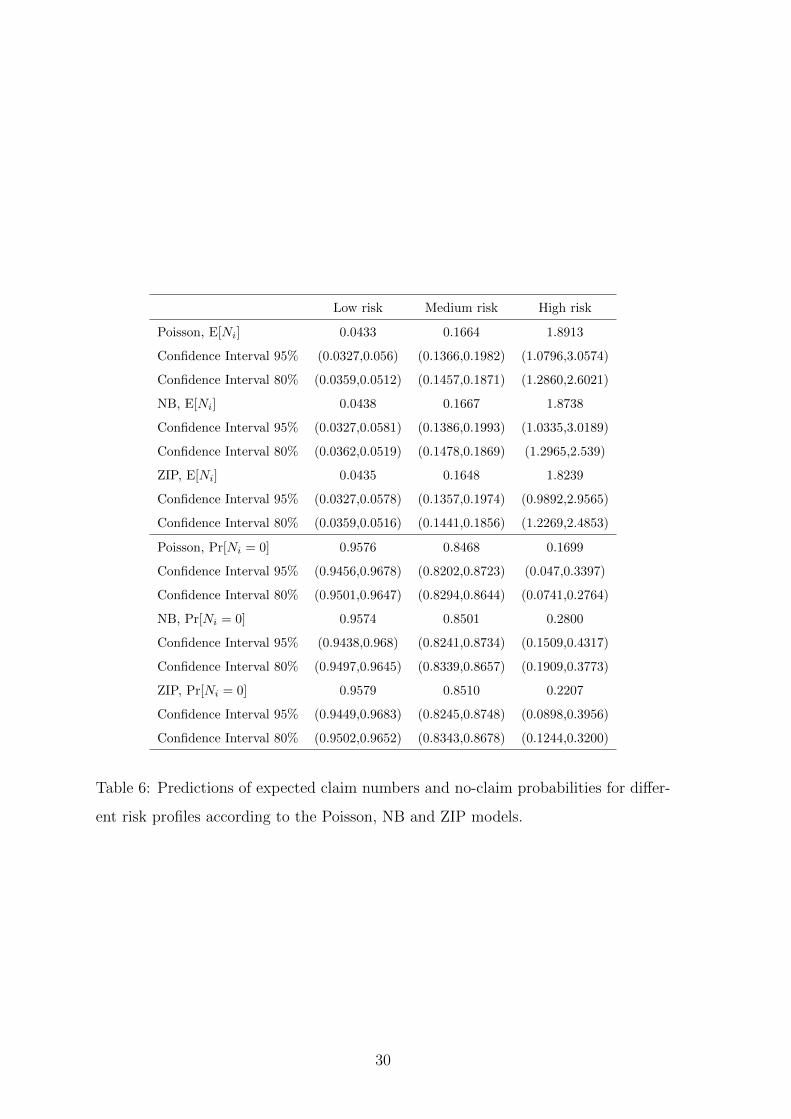
Table 6 gives the no-claim probability predicted by the Poisson, NB and ZIP models
for the following three risk profiles:
• high risk: unexperienced male driver aged 18 living in Brussels, driving a brand
new, gasoline, powerful car (power 200), occupying the initial level 11 in the
bonus-malus scale, subscribing TPL only.
• medium risk: middle-aged male driver aged 40 living in Liege driving a 4-year
diesel car with power 100, occupying level 2 in the bonus malus scale, subscribing
TPL+limited material damage and theft.
• low risk: retired male driver aged 70 living in the countryside, driving a 15-
year gasoline car with power 30, occupying level 0 in the bonus malus scale,
subscribing TPL+comprehensive coverage.
No vehicle belongs to a fleet and all policies are assumed to be in force for the whole
year.
As we can see from Table 6, the three models provide similar values for the expected
number of claims. This is also the case for no-claim probabilities, except for the high
risk profile where the Poisson model tends to underestimate this actuarial quantity,
making this profile less attractive at renewal compared to NB and ZIP models.
3.4.2 Credibility updates
In the Negative Binomial case, the probability density function of Θi given Ni = k is
exp (−θi (δi + µi)) θδi+k−1i∫ +∞
0exp (−ξ (δi + µi)) ξδi+k−1dξ
= exp (−θi (δi + µi)) θδi+k−1i
(δi + µi)δi+k
Γ (δi + k),
so that Θi given Ni = k obeys the Gamma distribution with updated parameter
values δi + k and δi + µi. Therefore, the expected relative risk level revised on the
basis of past experience is given by
E[Θi|Ni = k] =δi + k
δi + µi.
If the risk profile remains unchanged for the next year, the predicted expected claim
number µi is replaced with its update µi E[Θi|Ni = k] based on the information
29
Low risk Medium risk High risk
Poisson, E[Ni] 0.0433 0.1664 1.8913
Confidence Interval 95% (0.0327,0.056) (0.1366,0.1982) (1.0796,3.0574)
Confidence Interval 80% (0.0359,0.0512) (0.1457,0.1871) (1.2860,2.6021)
NB, E[Ni] 0.0438 0.1667 1.8738
Confidence Interval 95% (0.0327,0.0581) (0.1386,0.1993) (1.0335,3.0189)
Confidence Interval 80% (0.0362,0.0519) (0.1478,0.1869) (1.2965,2.539)
ZIP, E[Ni] 0.0435 0.1648 1.8239
Confidence Interval 95% (0.0327,0.0578) (0.1357,0.1974) (0.9892,2.9565)
Confidence Interval 80% (0.0359,0.0516) (0.1441,0.1856) (1.2269,2.4853)
Poisson, Pr[Ni = 0] 0.9576 0.8468 0.1699
Confidence Interval 95% (0.9456,0.9678) (0.8202,0.8723) (0.047,0.3397)
Confidence Interval 80% (0.9501,0.9647) (0.8294,0.8644) (0.0741,0.2764)
NB, Pr[Ni = 0] 0.9574 0.8501 0.2800
Confidence Interval 95% (0.9438,0.968) (0.8241,0.8734) (0.1509,0.4317)
Confidence Interval 80% (0.9497,0.9645) (0.8339,0.8657) (0.1909,0.3773)
ZIP, Pr[Ni = 0] 0.9579 0.8510 0.2207
Confidence Interval 95% (0.9449,0.9683) (0.8245,0.8748) (0.0898,0.3956)
Confidence Interval 80% (0.9502,0.9652) (0.8343,0.8678) (0.1244,0.3200)
Table 6: Predictions of expected claim numbers and no-claim probabilities for differ-
ent risk profiles according to the Poisson, NB and ZIP models.
30

contained in the number k of claims filed by policyholder i. The theoretical bonus-
malus coefficients E[Θi|Ni = k] exhibit some well-known features (see, e.g., Denuit et
al., 2007):
• the a posteriori corrections become more severe when the residual heterogeneity,
measured by Var[Θi], increases.
• considering two policyholders (numbered i1 and i2) such that i1 is a priori a
better driver than i2, that is, µi1 < µi2 ,
– if these policyholders do not report any claim (i.e., Ni1 = Ni2 = 0) then
the a priori worse driver receives more discount provided δi1 = δi2 .
– if these policyholders report k ≥ 1 claims (i.e., Ni1 = Ni2 = k) then the
penalty for the a priori bad driver is less severe than for the good one
provided δi1 = δi2 .
Compared to this classical setting, we have here a new effect coming from the respec-
tive values of δi1 and δi2 which may interfere with the preceding discussion.
Table 7 gives the theoretical bonus malus correction E[Θi|Ni = k] for the three risk
profiles according to the value of k and Table 8 displays the corresponding revised
expected claim frequencies. Considering the three risk profiles defined previously, we
know from Table 3 that δ tends to be larger for diesel vehicles compared to gasoline
ones and smaller for the vehicles covered in TPL only or in TPL+limited material
damage and theft compared to vehicles with comprehensive coverage. The spatial
variation in δ displayed in Figure 4 has no significant impact on the three risk profiles
we consider here. Including the intercept and the exposure-to-risk gives estimated
values of δ equal to exp(2.09) for the low risk profile, exp(1.18) for the medium risk
profile, and exp(0.81) for the high risk profile. Hence, the past claim experience plays
a more important role as the quality of the risk deteriorates, which conforms with
actuarial intuition.
If the low risk profile does not report any accident during the first year, we see
from Table 7 that the revision consists in multiplying the expected claim frequency
by 99.27%. This modest decrease is to be compared with the corresponding values
95.09% for the medium risk profile and 52.97% for the high risk profile. The discounts
31

Low risk
k E[Θi|Ni = k] Confidence Interval 95% Confidence Interval 80%
0 0.9927 (0.9815,0.9993) (0.9866,0.9984)
1 1.1617 (1.0172,1.4034) (1.0349,1.293)
2 1.3307 (1.0351,1.8257) (1.0715,1.6001)
3 1.4997 (1.0531,2.2479) (1.1081,1.905)
4 1.6688 (1.0711,2.6702) (1.1448,2.21)
5 1.8378 (1.089,3.0925) (1.1814,2.5165)
Medium risk
k E[Θi|Ni = k] Confidence Interval 95% Confidence Interval 80%
0 0.9509 (0.923,0.9733) (0.9348,0.9669)
1 1.2459 (1.1387,1.3773) (1.1717,1.327)
2 1.5409 (1.305,1.8292) (1.3752,1.7167)
3 1.8359 (1.4703,2.2851) (1.5786,2.105)
4 2.131 (1.6356,2.7356) (1.7831,2.4988)
5 2.426 (1.8009,3.1861) (1.9874,2.8907)
High risk
k E[Θi|Ni = k] Confidence Interval 95% Confidence Interval 80%
0 0.5297 (0.338,0.6975) (0.4079,0.6455)
1 0.7889 (0.5824,0.991) (0.6566,0.9174)
2 1.048 (0.796,1.3009) (0.8813,1.2135)
3 1.3072 (0.9963,1.6561) (1.0974,1.5229)
4 1.5664 (1.1922,2.0188) (1.3166,1.8275)
5 1.8256 (1.3854,2.3749) (1.5235,2.1403)
Table 7: Theoretical bonus malus correction E[Θi|Ni = k] for different risk profiles.
32

Low risk
k µi E[Θi|Ni = k] Confidence Interval 95% Confidence Interval 80%
0 0.0434 (0.0324,0.0577) (0.036,0.0514)
1 0.0508 (0.0367,0.0694) (0.0411,0.0614)
2 0.0581 (0.0394,0.0867) (0.0448,0.0733)
3 0.0654 (0.0407,0.1052) (0.0473,0.0866)
4 0.0728 (0.0415,0.1229) (0.0491,0.0993)
5 0.0801 (0.0427,0.1392) (0.0513,0.1129)
Medium risk
k µi E[Θi|Ni = k] Confidence Interval 95% Confidence Interval 80%
0 0.1584 (0.132,0.188) (0.1408,0.1769)
1 0.2075 (0.1701,0.254) (0.1816,0.2352)
2 0.2567 (0.2003,0.3267) (0.217,0.2977)
3 0.3058 (0.2277,0.4036) (0.251,0.3612)
4 0.3549 (0.2575,0.4781) (0.286,0.4261)
5 0.4041 (0.2868,0.558) (0.3192,0.4905)
High risk
k µi E[Θi|Ni = k] Confidence Interval 95% Confidence Interval 80%
0 0.958 (0.6408,1.3239) (0.7384,1.1807)
1 1.4283 (1.0242,1.8487) (1.1769,1.6907)
2 1.8986 (1.3382,2.3944) (1.563,2.2394)
3 2.3689 (1.6642,3.0078) (1.922,2.8068)
4 2.8392 (1.9959,3.6243) (2.2817,3.3782)
5 3.3095 (2.2739,4.2618) (2.6371,3.9529)
Table 8: Resulting revised expected claim frequency µi E[Θi|Ni = k] for different risk
profiles.
33

awarded to policyholders who do not report any accident to the insurance company are
thus increasing with the a priori annual expected claim frequency: The more claims
are expected by the insurance company on the basis of observable characteristics, the
higher the discount in case no claims are reported. This classical effect is amplified
here by the values of δ which put more weight on past experience for higher risk
profiles. Note however from Table 8 that the revised expected claim frequency is still
larger the higher the risk profile.
Now, considering the penalty in case one claim is reported, we see that when the low
risk profile reports one claim, the expected claim frequency is multiplied by 116.17%.
The corresponding values for the medium risk profile and for the high risk profile are
124.59% and 78.89%, respectively. The penalties in case an accident is reported to
the company are thus decreasing with the a priori annual expected claim frequencies.
Compared to the classical analyses where reporting a claim typically entails a penalty
comprised between 50 and 75%, we see that the present system based on accurate
risk classification appears to be less severe, and thus easier to implement in practice.
Moreover, the high risk profile still receives a discount in case only one claim is
reported, the penalty appearing when 2 or more claims are filed. Similar comments
apply when more claims are reported, i.e. for higher values of k. The corresponding
revised expected claim frequencies are displayed in Table 8.
Let us now consider the ZIP model. In this case, Θi is Bernoulli distributed with
mean 1− πi and
Pr[Θi = 0|Ni = ki] =
Pr[Θi=0]Pr[Ni=0]
= πiπi+(1−πi) exp(−λi) if ki = 0
0 if ki ≥ 1.
If Ni = 0 then the number of claims for next year is still ZIP with increased probability
mass at zero given by Pr[Θi = 0|Ni = 0]. If Ni ≥ 1 then the number of claims for next
year becomes Poisson distributed with mean λi and no further re-evaluation based on
claim experience is needed. As these re-evaluations are rather crude, the ZIP model
does not provide accurate enough credibility updates for claim frequencies and the
NB model is preferable.
34

4 Modelling Claim Sizes: Zero-Adjusted Regres-
sion
4.1 From individual to aggregate claim sizes
Large claims generally affect liability coverages. These major claim sizes require a
separate analysis as no simple standard parametric model seems to emerge as provid-
ing an acceptable fit to both small and large claims. Let us nevertheless mention the
composite models considered, e.g., in Pigeon and Denuit (2011) which can accomo-
date a mix of small and large claims but for which no regression analysis is available,
yet. Here, we restrict the analysis to observations with total claim size less than
exp(15) which corresponds to a threshold approximately equal to EUR 80,000 (or 3.2
millions Belgian francs) in the spirit of Cebrian et al. (2003).
With the noticeable exception of Jørgensen and Paes de Souza (1994), the vast ma-
jority of actuarial analyses of the pure premium so far have examined frequencies and
severities separately. The Tweedie GLM used by these authors is however quite re-
strictive as the no-claim probability is not allowed to depend on covariates. Heller et
al. (2007) extended this approach to Poisson, ZIP or NB claim frequencies combined
with Gamma or Inverse-Gaussian severities. The Tweedie distribution appears as a
special case corresponding to the Poisson-Gamma choice. In this section, we target
the total annual claim amount using zero-adjusted regression models. This provides
an alternative to these mixed Poisson compound models.
Before the Poisson regression became popular among actuaries, claims data were often
analyzed using logistic regression; see, e.g., Beirlant et al. (1991). Zero-adjusted
models are closely related to this approach but avoid the two-step analysis. As the
likelihood factors in two parts, one with the probability of reporting no claim and
another one with positive claim amounts, the two strategies lead to very similar
results. But analyzing the total claim amount by means of a single zero-adjusted
regression model allows the actuary to get accurate confidence intervals for several
key risk indicators, such as the expected claim cost, for instance. Confidence intervals
are more difficult to derive in the two-step approach because estimation errors from
the zero part and from the continuous part need to be combined. Moreover, it is not
35

that easy to obtain global DIC values when performing separate analyzes.
4.2 Zero-adjusted models
Zero-adjusted (ZA) models are discrete-continuous distributions with a probability
mass at zero and a continuous component which can be any parametric distribution
as long as first and second derivative of the log-likelihood can be computed. Therefore,
these models additionally allow to estimate the probability for positive claim sizes.
The idea of using such models to describe insurance data goes back to Heller et al.
(2006) who applied the zero-adjusted Inverse-Gaussian distribution as a model for
claim sizes, including zero claims. Whereas these authors confined to linear effects
of the covariates (a logit-linear model for the occurrence of a claim and log-linear
models for the expected claim size and for its dispersion when at least one claim is
reported), we allow here for nonlinear effects of the explanatory variables, including
spatial effects.
Consider the total claim sizes Yi and covariate vectors as in the previous section. The
distribution of Yi is defined by Pr[Yi = 0] = 1− πi and, given Yi > 0 (which happens
with probability πi) Yi has probability density function g(·) corresponding to some
continuous distribution with support in R+. Here, 1− πi is the no-claim probability,
not to be confused with the parameter πi in the ZIP model.
This representation corresponds to the individual model of risk theory. See, e.g.,
Chapter 2 in Kaas et al. (2008) for an introduction. In this model, the total claim
cost is decomposed into the product of an indicator for the event “the policy produces
at least one claim during the reference period” and a positive random variable repre-
senting the total claim amount produced by the policy when at least one claim has
been filed. This exactly corresponds to the construction of the ZA models. Numerous
powerful actuarial techniques have been developed for the individual model, which
are thus directly applicable to the ZA modeling output and facilitates the actuarial
analysis.
36

4.3 Numerical illustration
To model the total claim size, we used the LogNormal (LN), Gamma (GA) and
Inverse-Gaussian (IG) distribution supplemented with a probability mass at zero.
This allows for the simultaneous estimation of characteristics of the claim size distri-
bution and the no-claim probability. Explanatory variables are included in the three
parameters, the probability mass at zero 1 − π as well as both parameters of these
three continuous distributions. We use log link functions for positive parameters and
the identity link for the real-valued parameter of the LogNormal distribution. For the
claim probability π, the complementary log log link has been used. As for claim fre-
quencies, all models are compared graphically applying normalized quantile residuals
and by proper scoring rules. Predictor specifications were chosen by DIC together
with significances of the effects as described before. The spatial effect is modeled in
the spirit of Lang et al. (2013) consisting of a Markov random field and an additional
independent and identically distributed random effect.
Figure 9 shows the normalized quantile residuals computed from the subset of ob-
servations with positive claims. The residuals indicate that LN and IG are better
assumptions than the GA distribution since the residuals of the former two are very
close to the diagonal while the sample quantiles of the GA distribution greater than
3 are higher than the theoretical quantiles. This indicates that the GA model may
only be appropriate for modeling small claim sizes.
In Table 9, the computed scores and the DIC underline the preferences for applying
either the ZALN model (which would be chosen by DIC as well as the logarithmic,
quadratic and spherical score) or the ZAIG (with highest CRPS).
Model Brier Score Logarithmic Score Spherical Score CRPS DIC
ZALN 105,610.7 -171,614.4 125,911.6 -134,845.7 90,202
ZAIG 103,211.7 -172,983.5 124,908.4 -127,940.1 90,323
ZAGA 104,931.5 -174,303.7 125,533.1 -148,244.3 94,064
Table 9: Summarized scores from a ten-fold cross validation and DIC obtained from
estimations of the whole data set, optimal values appearing printed in bold.
For further illustration of this score, we performed a quantile decomposition and plot-
ted the scores against the quantiles in Figure 10. It gets obvious that for quantiles
37

Figure 9: Comparison of quantile residuals in the LogNormal, Inverse Gaussian and
Gamma model.
0.0 0.2 0.4 0.6 0.8 1.0
−1.
5−
1.0
−0.
50.
0
Quantile decomposition (zero−adjusted models)
Quantile
ZALNZAGAZAIG
Figure 10: Quantile decomposition of the CRPS.
smaller than 0.2 and greater than 0.9 the scores of ZALN and ZAIG are very similar,
while in between the ZAIG model delivers smaller losses. In a nutshell it can be
concluded that both the ZALN and ZAIG distributions seem to be very promising
candidates for the aggregate claim size distributions. For illustration and interpreta-
tion of effects we choose the ZALN model in the remainder of this section.
Given that the total claim size Yi is positive, we get
E[Yi|Yi > 0] = exp
(µi +
σ2i
2
)Var[Yi|Yi > 0] = exp
(2µi + σ2
i
)(exp(σ2
i )− 1).
Here, exp(µi) corresponds to the median claim cost when at least one claim has been
reported.
38

Based on the DIC we specified the following predictor structures for the location
parameter µcosts = ηµcosts ∈ R and scale parameter σ2costs = exp
(ησ
2
costs
)> 0. Here,
ηµcosts = fµ1 (ageph) + sex fµ2 (ageph) + fµ3 (agec) + fµ4 (bm) + fµspat(distr) + (zµ)′ βµ,
where zµ consists of fleet , coverage and an overall constant. For σ2 we get
ησ2
costs = fσ2
1 (ageph) + fσ2
spat(distr) +(zσ
2)′βσ
2
,
where zσ2
consists of fleet , coverage and an intercept.
For πcosts, we follow again Baetschmann and Winkelmann (2012) since there are sev-
eral policyholders with a contract shorter than one year and we choose
πcosts = 1− exp(− exp(ηπcosts)). (6)
It is instructive to compare the specifications (5) and (6): In the ZIP case π mod-
els the probability of observing structural zeros (compare Section 3.2) while in the
ZALN model π stands for the probability of observing a positive claim size, i.e.
πi = Pr[Yi > 0]. Therefore, equations (5) and (6) are reasonable since an increasing
contract period, included in the predictor, reduces π in the ZIP model and raises the
probability of observing a positive claim connected with a positive amount. Based
on this specification, we found as best predictor specification
ηπcosts = fπ1 (ageph)+sex fπ2 (ageph)+fπ3 (agec)+fπ4 (power)+fπ5 (bm)+fπspat(distr)+(zπ)′ βπ,
where zπ consists of fuel , fleet , coverage an intercept and the logarithm of the contract
period in days.
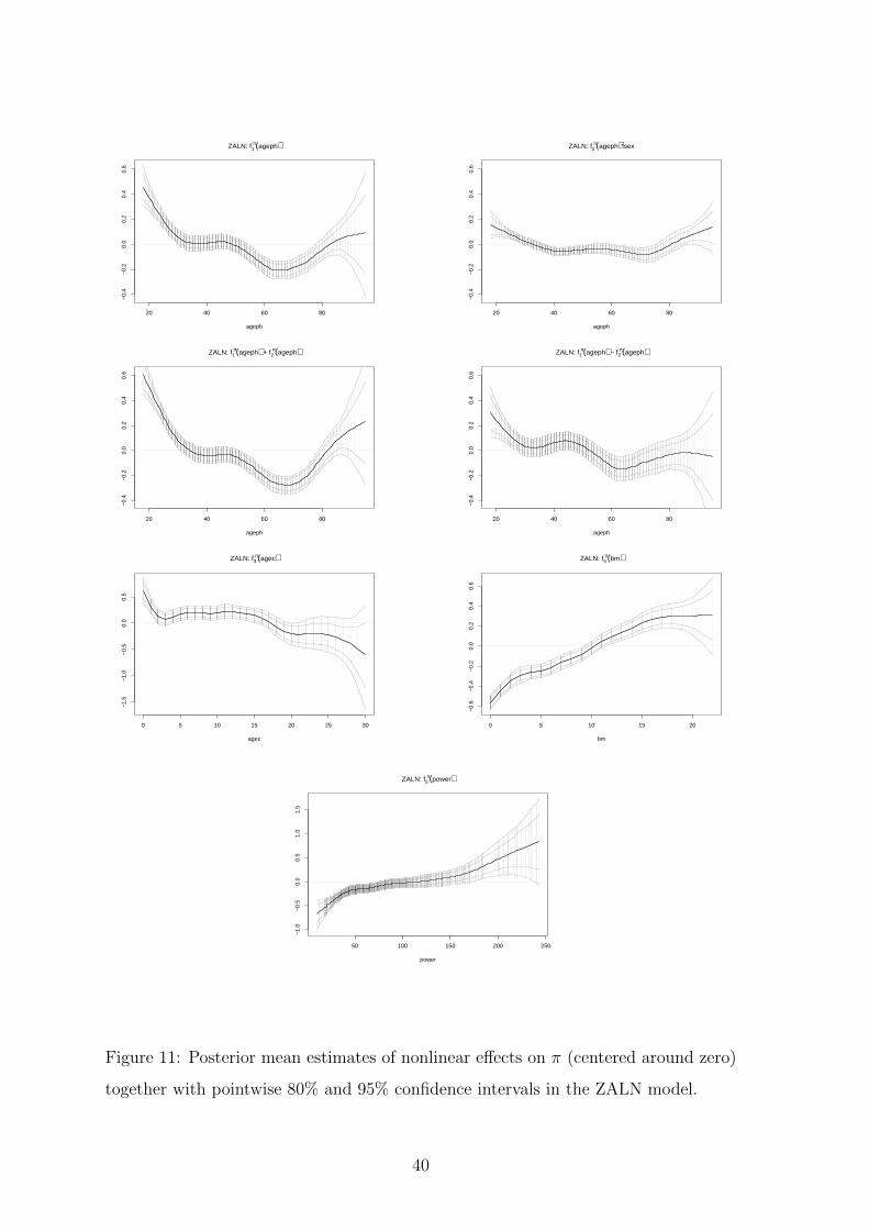
Figure 14 depicts the estimated spatial effects on µ, σ2 and π. Estimates of nonlinear
effects are shown in Figures 11, 12 and 13 while Table 10 summarizes all linear effects.
Considering the effects of the categorical covariates on the claim probability π, we see
from Table 10 that driving a diesel vehicle decreases the no-claim probability whereas
belonging to a fleet increases this probability. Also, extending the coverage increases
the no-claim probability. As expected, all estimated nonlinear effects on π are quite
similar to the ones we estimated in the ZIP model, so that the same comments apply
here, mutatis mutandis. This can be explained by the large number of policyholders
who either report no or only one claim. For the spatial effects, we can summarize
39
20 40 60 80
−0.4
−0.2
0.0
0.2
0.4
0.6
ZALN: f1 π(ageph)
ageph
20 40 60 80
−0.4
−0.2
0.0
0.2
0.4
0.6
ZALN: f2 π(ageph)*sex
ageph
20 40 60 80
−0.4
−0.2
0.0
0.2
0.4
0.6
ZALN: f1 π(ageph) + f2
π(ageph)
ageph
20 40 60 80
−0.4
−0.2
0.0
0.2
0.4
0.6
ZALN: f1 π(ageph) − f2
π(ageph)
ageph
0 5 10 15 20 25 30
−1.5
−1.0
−0.5
0.0
0.5
ZALN: f3 π(agec)
agec
0 5 10 15 20
−0.6
−0.4
−0.2
0.0
0.2
0.4
0.6
ZALN: f4 π(bm)
bm
50 100 150 200 250
−1.0
−0.5
0.0
0.5
1.0
1.5
ZALN: f5 π(power)
power
Figure 11: Posterior mean estimates of nonlinear effects on π (centered around zero)
together with pointwise 80% and 95% confidence intervals in the ZALN model.
40

20 40 60 80
0.0
0.5
1.0
ZALN: f1 µ(ageph)
ageph
20 40 60 80
0.0
0.5
1.0
ZALN: f2 µ(ageph)*sex
ageph
20 40 60 80
0.0
0.5
1.0
ZALN: f1 µ(ageph) + f2
µ(ageph)
ageph
20 40 60 80
0.0
0.5
1.0
ZALN: f1 µ(ageph) − f2
µ(ageph)
ageph
0 5 10 15 20 25 30
−1.5
−1.0
−0.5
0.0
0.5
ZALN: f3 µ(agec)
agec
0 5 10 15 20
−0.4
−0.2
0.0
0.2
ZALN: f4 µ(bm)
bm
Figure 12: Posterior mean estimates of nonlinear effects on µ (centered around zero)
together with pointwise 80% and 95% confidence intervals in the ZALN model
20 40 60 80
−0.6
−0.4
−0.2
0.0
0.2
ZALN: f1 σ2(ageph)
ageph
Figure 13: Posterior mean estimates of nonlinear effects on σ2 (centered around zero)
together with pointwise 80% and 95% confidence intervals in the ZALN model.
41

ZALN: Estimated spatial effect on π
−0.53 0.530
ZALN: 80% posterior probabilites of spatial effect on π
−1 10
ZALN: Estimated spatial effect on µ
−0.23 0.230
ZALN: 80% posterior probabilites of spatial effect on µ
−1 10
ZALN: Estimated spatial effect on σ2
−0.23 0.230
ZALN: 80% posterior probabilites of spatial effect on σ2
−1 10
Figure 14: Estimated posterior mean complete spatial effects in the ZALN model
(centered around zero) together with corresponding probability plots.
42
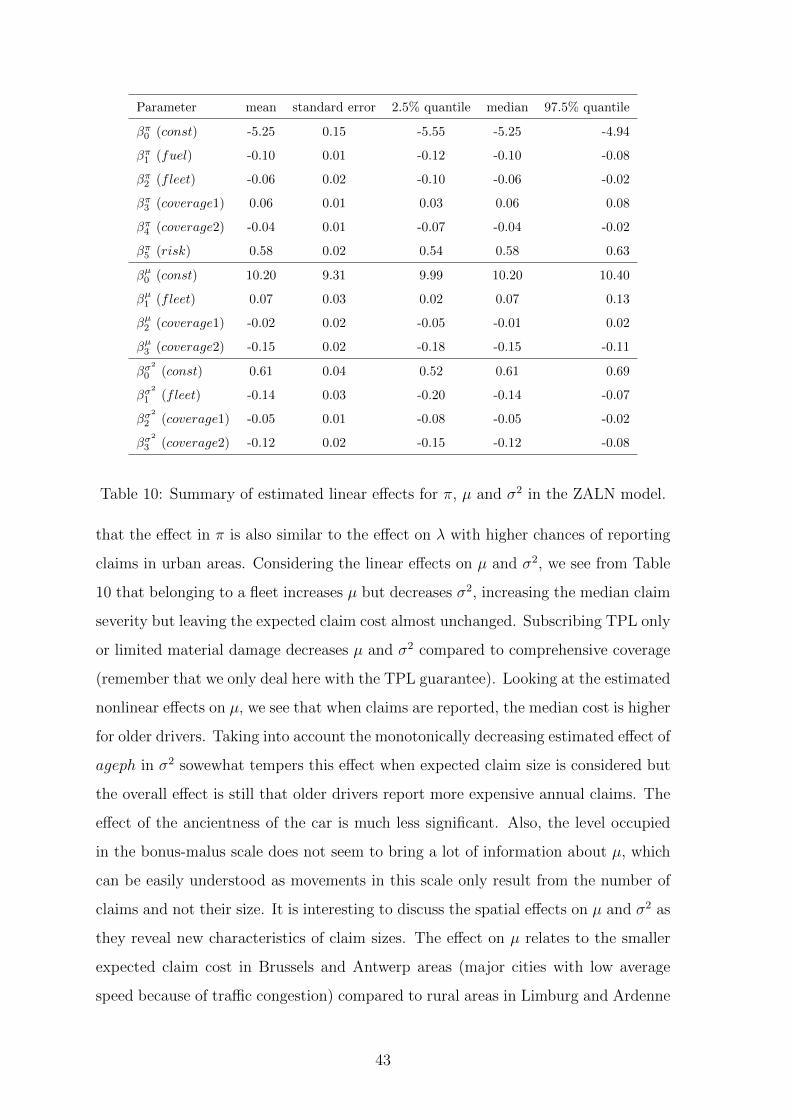
Parameter mean standard error 2.5% quantile median 97.5% quantile
βπ0 (const) -5.25 0.15 -5.55 -5.25 -4.94
βπ1 (fuel) -0.10 0.01 -0.12 -0.10 -0.08
βπ2 (fleet) -0.06 0.02 -0.10 -0.06 -0.02
βπ3 (coverage1) 0.06 0.01 0.03 0.06 0.08
βπ4 (coverage2) -0.04 0.01 -0.07 -0.04 -0.02
βπ5 (risk) 0.58 0.02 0.54 0.58 0.63
βµ0 (const) 10.20 9.31 9.99 10.20 10.40
βµ1 (fleet) 0.07 0.03 0.02 0.07 0.13
βµ2 (coverage1) -0.02 0.02 -0.05 -0.01 0.02
βµ3 (coverage2) -0.15 0.02 -0.18 -0.15 -0.11
βσ2
0 (const) 0.61 0.04 0.52 0.61 0.69
βσ2
1 (fleet) -0.14 0.03 -0.20 -0.14 -0.07
βσ2
2 (coverage1) -0.05 0.01 -0.08 -0.05 -0.02
βσ2
3 (coverage2) -0.12 0.02 -0.15 -0.12 -0.08
Table 10: Summary of estimated linear effects for π, µ and σ2 in the ZALN model.
that the effect in π is also similar to the effect on λ with higher chances of reporting
claims in urban areas. Considering the linear effects on µ and σ2, we see from Table
10 that belonging to a fleet increases µ but decreases σ2, increasing the median claim
severity but leaving the expected claim cost almost unchanged. Subscribing TPL only
or limited material damage decreases µ and σ2 compared to comprehensive coverage
(remember that we only deal here with the TPL guarantee). Looking at the estimated
nonlinear effects on µ, we see that when claims are reported, the median cost is higher
for older drivers. Taking into account the monotonically decreasing estimated effect of
ageph in σ2 sowewhat tempers this effect when expected claim size is considered but
the overall effect is still that older drivers report more expensive annual claims. The
effect of the ancientness of the car is much less significant. Also, the level occupied
in the bonus-malus scale does not seem to bring a lot of information about µ, which
can be easily understood as movements in this scale only result from the number of
claims and not their size. It is interesting to discuss the spatial effects on µ and σ2 as
they reveal new characteristics of claim sizes. The effect on µ relates to the smaller
expected claim cost in Brussels and Antwerp areas (major cities with low average
speed because of traffic congestion) compared to rural areas in Limburg and Ardenne
43

(with weaker traffic intensity and higher average speed resulting in more expensive
accidents when they occur). This main effect is refined by the spatial structure in
σ2, somewhat increasing the expected claim severities in some urban districts and
decreasing the average claim cost in Wallonia compared to Flanders and Brussels.
This might be explained by the higher living standards in Flanders and Brussels
where more expensive cars may be driven, increasing the average claim size.
Low risk Medium risk High risk
ZALN, E[Yi] 3965.87 5699.8 88031.46
Confidence Interval 95% (2620.23,5833) (4246.14,7566.32) (49504.56,150846.18)
Confidence Interval 80% (2969.85,5044.94) (4674.02,6758.25) (58426.16,121233.93)
ZALN, πi = Pr[Yi > 0] 0.0425 0.1522 0.7801
Confidence Interval 95% (0.032,0.0548) (0.1274,0.1798) (0.5867,0.9383)
Confidence Interval 80% (0.0351,0.0501) (0.1353,0.1706) (0.6617,0.8896)
ZALN, µi = E[log(Yi)|Yi > 0] 10.3627 9.6232 10.1496
Confidence Interval 95% (10.1217,10.5796) (9.4573,9.7911) (9.8048,10.5242)
Confidence Interval 80% (10.2165,10.5127) (9.5106,9.7353) (9.923,10.3756)
ZALN, σ2i = Var[log(Yi)|Yi > 0] 2.1375 1.802 2.8976
Confidence Interval 95% (1.6951,2.6315) (1.5231,2.0831) (2.2863,3.6579)
Confidence Interval 80% (1.8561,2.4481) (1.6246,1.9902) (2.4674,3.3468)
Table 11: Predictions of expected claim amounts in Belgian francs (1EUR being
approximately equal to 40 Belgian francs) and of parameters π, µ and σ2 for different
risk profiles in the ZALN model.
Table 11 displays the predictions obtained from the ZALN model for the three risk
profiles defined earlier in the paper. Again, we discover there new features of the
insurance data set as the three risk profiles greatly differ in their respective no-claim
probabilities but not that much on the expected claim size when claims are reported.
We see from Table 11 that E[Yi|Yi > 0] is similar for the low and high risk profiles,
but smaller for the medium risk profile. This conforms with actuarial intuition: Indi-
vidual drivers’ characteristics are more efficient at explaining the number of reported
TPL claims than their corresponding costs which depend to a large extent on the
third party involved. Considering the variations in the no-claim probabilities, we
nevertheless end up with an expected claim cost E[Yi] which increases with the risk
profile considered.
44
5 Discussion
The present paper extends the study conducted by Denuit and Lang (2004) to gener-
alized additive models for location, scale and shape (GAMLSS). This flexible, semi-
parametric class of regression models turns out to be particularly suitable for analyz-
ing insurance data. The restrictive exponential family assumption for the response
is relaxed compared to standard GLM-based analysis which opens the door to nu-
merous response distributions in line with the specificities of insurance data. While
ordinary regression analyzes only the effects of covariates on the mean of a response,
the approach proposed in the present paper allows the actuary to include risk factors
not only in the mean but also in other parameters governing the claiming behavior,
like the degree of residual heterogeneity or the no-claim probability. In this broader
setting, the Poisson assumption made in Denuit and Lang (2004) is replaced with a
mixed Poisson one, either the Negative Binomial distribution with cell-specific het-
erogeneity or the zero-inflated Poisson distribution with cell-specific probability mass
at zero. Bayesian inference is based on efficient Markov chain Monte Carlo simu-
lation techniques with appropriate proposal densities based on iteratively weighted
least square approximations to the full conditionals. In this way, simultaneous estima-
tion of possible nonlinear effects, spatial variations, random effects and interactions
between risk factors within the data set are possible.
In addition to these models for claim frequencies, new models for claim severities are
also presented, either per claim or aggregated per year. In the former case, location
and scale parameters in the LogNormal, Gamma or Inverse Gaussian distributions
may depend on covariates. Total claim amounts distributions are then obtained by
combining estimated frequencies with estimated claim sizes by means of Panjer al-
gorithm, for instance. In the latter case, an additional probability mass is placed at
zero, corresponding to the policies without claims, allowing the actuary to account
for zeros in the analysis of the amount of loss directly without resorting to models for
claim frequencies. This yields zero-adjusted LogNormal, Gamma or Inverse Gaussian
distributions able to deal with the large number of zero observations within the insur-
ance data sets. Such zero-adjusted models based on distributions with a probability
mass at zero and a continuous component thus allow for analyzing claim sizes in due
45

consideration of claim-free policyholders. In all cases, linear and nonlinear effects of
the covariates can be accounted for, with or without parametric formulation in the
latter case. Interactions between risk factors are allowed and spatial correlations as
well as unobserved heterogeneity can be captured.
To illustrate the relevance of this approach, we performed a detailed illustrative anal-
ysis based on the Belgian motor insurance portfolio studied in Denuit and Lang
(2004). These highly flexible regression models reveal new features of insurance data
and have important consequences for a priori risk management and for credibility
updating mechanisms. Guidelines for model choice with respect to the response dis-
tributions and for further model specifications are also provided. For the comparison
of models with respect to the distribution, we consider quantile residuals as an effec-
tive graphical device and scoring rules that allow to quantify the predictive ability of
the models. The deviance information criterion is used for further model specification.
To end with, let us mention that GAMLSS models have numerous additional poten-
tial applications to insurance. For instance, the GAMLSS family includes the Beta
distribution inflated at 0, at 1 or at 0 and 1. This framework is thus appropriate to
model material damage claims which are expressed as a percentage of the sum insured
(the value of the insured vehicle, in motor insurance). Applications to life and health
insurance are also promising, in the spirit of Gschlossl et al. (2011).
References
Baetschmann, G., Winkelmann, R., 2012. Modelling zero-inflated count data when exposure varies
with an application to sick leave. Technical Report.
Beirlant, J., Derveaux, V., De Meyer, A.M., Goovaerts, M.J., Labies, E., Maenhoudt, B., 1991. Sta-
tistical risk evaluation applied to (Belgian) car insurance. Insurance: Mathematics and Economics
10, 289-302.
Bortoluzzo, A.B., Claro, D.P., Caetano, M.A.L., Artes, R., 2011. Estimating total claim size in
the auto insurance industry: A comparion between Tweedie and zero-adjusted Inverse Gaussian
distribution. Brazilian Administration Review 8, 37-47.
Boucher, J.-Ph., Denuit, M., Guillen, M., 2007. Risk classification for claim counts: A comparative
analysis of various zero-inflated mixed Poisson and hurdle models. North American Actuarial Journal
11, 110-131.
Brezger, A., Lang, S., 2004. Bayesian P-splines. Journal of Computational and Graphical Statistics
46

13, 183–212.
Brezger, A., Lang, S., 2006. Generalized structured additive regression based on Bayesian P-splines
Computational Statistics & Data Analysis 50, 967–991.
Cebrian, A., Denuit, M., Lambert, Ph., 2003. Generalized Pareto fit to the society of Actuaries
large claims database. North American Actuarial Journal 7, 18-36.
Denuit, M., Lang, S., 2004. Nonlife ratemaking with Bayesian GAM’s. Insurance: Mathematics and
Economics 35, 627-647.
Denuit, M., Marechal, X., Pitrebois, S., Walhin, J.-F., 2007. Actuarial Modelling of Claim Counts:
Risk Classification, Credibility and Bonus-Malus Systems. Wiley, New York.
Dunn, P.K., Smyth, G.K., 1996. Randomized quantile residuals. Computational and Graphical
Statistics 5, 236–245.
Eilers, P.H.C., Marx, B.D., 1996. Flexible smoothing using B-splines and penalized likelihood (with
comments and rejoinder). Statistical Science 11, 89-121.
Fahrmeir, L., Kneib, T., Lang, S., 2004. Penalized additive regression for space-time data: A
Bayesian perspective. Statistica Sinica 14, 713-743.
Fahrmeir, L., Lang, S., 2001a. Bayesian inference for generalized additive mixed models based on
Markov random field priors. Journal of the Royal Statistical Society – Series C 50, 201-220.
Fahrmeir, L., Lang, S., 2001b. Bayesian semiparametric regression analysis of multicategorical time-
space data. Annals of the Institute of Statistical Mathematics 53, 10-30.
Fahrmeir, L., Tutz, G., 2001. Multivariate Statistical Modelling Based on Generalized Linear Mod-
els. Springer-Verlag, New York.
Fahrmeir, L., Kneib, T., Lang, S., Marx, B., 2013. Regression - Models, Methods and Applications.
Springer.
Friedman, J.H., 1991. Multivariate adaptive regression splines (with discussion). Annals of Statistics
19, 1-141.
Gamerman, D., 1997. Sampling from the posterior distribution in Generalized Linear Mixed Models.
Statistics and Computing 7, 57–68.
George, A., Liu, J.W., 1981. Computer Solution of Large Sparse Positive Definite Systems. Prentice-
Hall.
Gneiting, T., Raftery, A.E., 2007. Strictly proper scoring rules, prediction, and estimation. Journal
of the American Statistical Association 102, 359–378.
Gneiting, T., Ranjan, R., 2011. Comparing density forecasts using threshold and quantile-weighted
scoring rules. Journal of Business & Economic Statistics 29, 411–421.
Green, P.J., 2001. A primer in Markov Chain Monte Carlo. In: Barndorff-Nielsen, O.E., Cox, D.R.,
Kluppelberg, C. (Eds.), Complex Stochastic Systems. Chapmann and Hall, London, pp. 1-62.
Gschlossl, S., Schoenmaekers, P., Denuit, M., 2011. Risk classification in life insurance: Methodology
and case study. European Actuarial Journal 1, 23-41.
47

Hastie, T., Tibshirani, R., 1990. Generalized Additive Models. Chapman and Hall, London.
Hastie, T., Tibshirani, R., 1993. Varying-coefficient models. Journal of the Royal Statistical Society
– Series B 55, 757-796.
Heller, G., Stasinopoulos, D. M., Rigby R. A., 2006. The zero-adjusted Inverse Gaussian distribution
as a model for insurance data. Proceedings of the 21th International Workshop on Statistical
Modelling, J. Hinde, J. Einbeck, J. Newell Editors, pp. 226-233.
Heller, G., Stasinopoulos, D. M., Rigby R. A., de Jong, P., 2007. Mean and dispersion modeling for
policy claim costs. Scandinavian Actuarial Journal, 281-292.
Jørgensen, B., Paes de Souza, M.C., 1994. Fitting Tweedie’s compound Poisson model to insurance
claims data. Scandinavian Actuarial Journal 69-93.
Jullion, A., Lambert, P., 2007. Robust specification of the roughness penalty prior distribution
in spatially adaptive Bayesian P-splines models. Computational Statistics & Data Analysis 51,
2542–2558.
Kaas, R., Goovaerts, M.J., Dhaene, J., Denuit, M., 2008. Modern Actuarial Risk Theory Using R.
Springer, New York.
Klein, N., Kneib, T., Lang, S., 2013a. Bayesian Generalized Additive Models for Loca-
tion, Scale and Shape for Zero-Inflated and Overdispersed Count Data. Technical Report,
http://econpapers.repec.org/paper/innwpaper/2013-12.htm.
Klein, N., Kneib, T., Lang, S., 2013b. Bayesian Structured Additive Distributional Regression.
Technical Report.
Klugman, S., Panjer, H., Willmot, G., 2004. Loss Models: From Data to Decisions. Wiley, New
York.
Lang, S., Brezger, A., 2004. Bayesian P-splines. Journal of Computational and Graphical Statistics
13, 183-212.
Lang, S., Umlauf, N., Wechselberger, P., Harttgen, K., Kneib, T., 2013. Multilevel Structured
Additive Regression. Statistics and Computing 23, in press.
Lin, X., Zhang, D., 1999. Inference in Generalized Additive Mixed Models by using Smoothing
Splines. Journal of the Royal Statistical Society – Series B 61, 381-400.
Ngo, L.,Wand, M.P., 2003. Smoothing with mixed model software. Journal of Statistical Software
9. Also available at http://www.maths.unsw.edu.au/Eœwand/.
Pigeon, M., Denuit, M., 2011. Composite Lognormal-Pareto model with random threshold. Scandi-
navian Actuarial Journal, 177-192.
Resti, Y., Ismail, N., Jamaan, S.H., 2013. Estimation of claim cost data using zero-adjusted Gamma
and Inverse Gaussian regression models. Journal of Mathematics and Statistics 9, 186-192.
Rigby, R.A., Stasinopoulos, D.M., 2005. Generalized additive models for location, scale and shape
(with discussion). Applied Statistics 54, 507–554.
Rue, H., Held, L., 2005. Gaussian Markov Random Fields. Chapman & Hall / CRC.
48

Ruppert, D., Wand, M.P., Carroll, R.J., 2003. Semiparametric Regression. Cambridge University
Press.
Spiegelhalter, D.J., Best, N.G., Carlin, B.P., Van der Linde, A., 2002. Bayesian measures of model
complexity and fits (with discussion). Journal of the Royal Statistical Society – Series B 64, 583-639.
Stasinopoulos, D.M., Rigby, R.A., 2007 Generalized additive models for location scale and shape
(GAMLSS) in R. Journal of Statistical Software 23, 1-46.
Stasinopoulos, D.M., Rigby, B., Akantziliotou, C., 2008. Instructions on how to use the gamlss
package in R, Second Edition.
Smyth, G.K., Jørgensen, B., 2002. Fitting Tweedie’s compund Poisson model to insurance claims
data: Dispersion modeling. Astin Bulletin 32, 143–157.
Wand, M.P., 2003. Smoothing and mixed models. Computational Statistics 18, 223-249.
Wood, S.N., 2000. Modelling and smoothing parameter estimation with multiple quadratic penalties.
Journal of the Royal Statistical Society – Series B 62, 413-428.
Wood, S.N., 2001. mgcv: GAMs and generalized ridge regression for R. R News 1, 20-25.
Wood, S.N., 2003. Thin plate regression splines. Journal of the Royal Statistical Society – Series B
65, 95-114.
Wood, S. N., 2004. Stable and efficient multiple smoothing parameter estimation for generalized
additive models. Journal of the American Statistical Association 99, 673–686.
Wood, S.N., 2006. Generalized Additive Models : An Introduction with R. Chapmann & Hall.
Wood, S. N., 2008. Fast stable direct fitting and smoothness selection for Generalized Additive
Models. Journal of the Royal Statistical Society – Series B 70, 495–518.
Yip, K.C.H., Yau, K.K.W., 2005. On modeling claim frequency data in general insurance with extra
zeros. Insurance: Mathematics and Economics 36, 153-163.
49