Extracting Progenitor Parameters of Rotating CCSNe via Pattern Recognition and MachineLearning

Laksh Bhasin1

Mentor: Alan Weinstein. Co-Mentor: Sarah Gossan.1LIGO SURF 2014, California Institute of Technology, 1200 E California Blvd., Pasadena, CA 91125, USA

AbstractCore-collapse supernovae (CCSNe) are among the most energetic events in the universe, releasing up to 1053 erg = 100 B ofgravitational potential energy. Based on theoretical predictions, they are also expected to emit bursts of gravitational waves(GWs) that will be detectable by second-generation laser interferometer GW observatories such as Advanced LIGO (aLIGO),Advanced Virgo, and KAGRA. In a novel pattern-recognition approach, we investigate the inference of progenitor parametersfrom numerical GW signals produced by state-of-the-art rotating core-collapse simulations. After associating physical processeswith characteristic spectrogram features, we develop several machine-learning (ML) algorithms that can accurately (oftenwithin ±20% relative error on average) and precisely determine progenitor parameters from optimally-oriented CCSN signalslocated 5 kpc away from Earth. In particular, our ±2σ prediction intervals for βic,b (the ratio of rotational kinetic energy togravitational energy of the inner core at bounce) are ∼ 0.03 wide on average at 5 kpc. At a source distance of 10 kpc, we stillachieve average relative errors within ±20% for our mean predictions, though our ±2σ prediction intervals for βic,b become∼ 0.05 wide. In addition to our hand-picked “physical” feature vector (FV) approach, we also investigate FV constructions withprincipal component analysis (PCA) and the scale-invariant feature transform (SIFT). In the future, our analysis could beimplemented in the aLIGO data analysis pipelines to help determine the inner core dynamics of the next galactic CCSN; thisinformation would otherwise be inaccessible via electromagnetic radiation.

I. Introduction

Towards the end of its hydrostatic-burning phase, a mas-sive star (i.e. 8 − 10M . M . 130M at zero-age mainsequence (ZAMS)) is composed of several concentric shellsthat represent its previous burning phases: hydrogen, helium,carbon, neon, oxygen, and silicon. As the silicon shell burns,an iron core starts to develop and increase in mass; whenthe mass of this core becomes sufficiently large, electron de-generacy pressure can no longer stabilize the core againstgravitational forces [1]. This triggers the collapse of the innercore, where material is compressed to supranuclear densitiesof ρ & ρ0 ∼ 2.7 × 1014 g/cm3. Due to the low compressibil-ity of nuclear matter (i.e. the stiffening of the equation ofstate) and the repulsive nature of the nuclear force, the innercore decelerates and starts to “bounce” back; this creates ahydrodynamic shock wave that propagates outwards untilit collides with the supersonically-infalling outer core (seeFigure 1, adapted from [1]). However, energy losses (e.g. todisassociation of heavy nuclei in the post-shock region) stallthe shock wave, and the wave must somehow be revived topass through the remaining outer core, produce a supernova(SN), and leave behind a neutron star. If this revival doesnot take place, black hole formation will occur instead of acore-collapse supernova (CCSN).As one of the most energetic processes in the universe –

releasing 1053 erg = 100 B of gravitational energy, ∼99% ofwhich is carried away by neutrinos [2] – core-collapse super-novae (CCSNe) are of high astrophysical significance. How-ever, while the above description is in general accurate, thetrue process that triggers the shock wave’s revival is not wellunderstood. The actual CCSN mechanism is believed tobe a combination of convection, rotation, neutrino heating,magnetic fields, and accretion shock instabilities.

To get a better understanding of the core dynamics in-volved in a CCSN, we can study the gravitational waves(GWs) emitted. These waves are emitted from dense nuclearregions that are impenetrable by photons, and carry valuableinformation about the progenitor’s parameters and its innercore’s physical processes. Moreover, unlike electromagneticwaves, they remain largely unaffected by intervening materialas they travel at the speed of light towards Earth.Rotating CCSNe are of particular interest to GW as-

tronomers, since the rotation in these progenitors leads to anoblate deformation of the collapsing core. As this deformedcore passes through the collapse and bounce phases, it un-dergoes extreme amounts of acceleration that in turn lead tostrong time-varying quadrupole moments. The resulting GWburst signal from pressure-driven core bounce can thereforebe fairly strong; for rapidly-rotating cores, it can be detectedby second-generation GW detectors out to > 10 kpc [3].

Recent estimates based on historical records of supernovaeand the simulated observability at a latitude of 35N suggesta galactic CCSN rate of 3.2+7.3

−2.6 per century [4]. Given thesechances of observability, it is therefore necessary to develop aset of tools that will let us analyze a given GW signature froma CCSN and determine the underlying progenitor parameters.Unfortunately, core collapse events in general cannot be han-dled with the same template search methods that have beensuccessful with binary inspiral mergers, since their resultingGW strains are dependent on many more variables (e.g. theequation of state (EOS) and neutrino transport schemes, bothof which are themselves highly parametrized). Since it is cur-rently not computationally feasible to cover the entire signalparameter space of CCSNe via numerical simulations, alter-native parameter estimation and waveform reconstructiontechniques have been developed.Many of these alternative techniques have focused on the

GW signal from rotating core collapse, as this tends to have

1

Figure 1: A schematic representation of the post-bounce shock-propagation stage that occurs during a core-collapsesupernova. The upper half of this image depicts dy-namical conditions, with arrows representing velocityvectors; these indicate a clear shock-wave expansionagainst gravitational collapse forces. The lower halfindicates the star’s nuclear composition and nuclearand weak processes; among these, we find neutrinobursts that result from the shock wave losing energy toneutrinos. The horizontal axis gives the enclosed massin M, and the vertical axis shows the correspondingradii in km (where RFe is the iron core radius and Rνis the neutrinosphere radius). Figure adapted from [1].

a relatively simple morphology. In particular, the signalconsists of a pre-bounce rise in the strain h, a large spike atbounce, and a brief (. 10 ms) postbounce ringdown [5] (see,for example, Figure 3). If we purely consider this rotation-induced segment of the GW signal, and ignore the ensuingstrains produced from convection, we can also make severalsimplifications in our parameter estimation problem. Forinstance, Dimmelmeier et al. [6], who considered two finite-temperature nuclear equations of state, found a fairly weakdependence of this GW signal on the EOS. Furthermore, arecent study by Ott et al. [3] established a phenomenon knownas the “universality of rotating core collapse.” Looking atboth 12M and 40M progenitors with the same precollapserotation rates, Ott et al. found fairly minimal differencesin the spectral GW energy density dEGW/df in the case ofeven moderate progenitor rotation. In fact, as Abdikamalovet al. [5] recently established, the morphology of the rotatingCCSN’s GW signal depends most noticeably on the angularmomentum of the precollapse core.

This relative simplicity of rotating CCSNe has recently beenleveraged by Engels et al. [7] for waveform reconstruction.After performing singular value decomposition (SVD) on theAbdikamalov catalog [5] to create a principal component (PC)basis of strain waveforms, Engels et al. used least-squaresregression to link physical parameters to members of the PCbasis. This allowed for an accurate prediction of waveformsgiven a set of physical progenitor parameters. Furthermore, in

the realm of parameter estimation, Abdikamalov et al. wereable to use matched filtering on noisy waveforms from theirown CCSN catalog to infer the total angular momentum ofthe inner core at bounce; their mean predictions achievedrelative errors within ±20%, assuming optimally-orientedprogenitors located 10 kpc away from Earth [5]. Edwardset al. [8] also managed to achieve accurate results on weakGW CCSN signals by using Bayesian techniques to regresscontinuous physical parameters on the PC basis from theAbdikamalov training catalog. With a separate set of noisyinjection waveforms, they then used their regression modelto fit physical parameters on the posterior means of the PCcoefficients. By applying this technique to waveforms withlow signal-to-noise ratios (SNRs) of 20, they achieved 90%confidence intervals for βic,b (the ratio of rotational kineticenergy to gravitational energy of the inner core at bounce)that were only ∼ 0.06 wide in the case of an unknown arrivaltime.

In this paper, we investigate a pattern-recognition/machine-learning (ML) approach to parameter estimation for rotatingCCSNe. In particular, we analyze the spectrogram-domain(time-frequency plane) and time-domain waveforms from theAbdikamalov catalog and identify key visual similarities anddifferences between GWs produced via different progenitors.By developing various image-processing and signal-processingalgorithms to automate this feature-identification process,and by combining these features into a feature vector (FV),we are able to simultaneously estimate various progenitorparameters of a given CCSN GW signal via ML techniques.Assuming optimally-oriented progenitors located D = 5 kpcfrom Advanced LIGO (aLIGO), the mean predictions of ourbest-performing algorithms tend to have relative errors within±20% for most waveforms in the Abdikamalov catalog. Fur-thermore, our ±2σ prediction intervals for βic,b are ∼ 0.03wide on average when D = 5 kpc; this width gives a reason-able estimate of the spread of our predictions due to differentaLIGO noise instantiations. At the fiducial galactic distanceof D = 10 kpc, our average predictions still remain within±20% of the true parameter values in terms of relative error,yet the ±2σ intervals for βic,b become ∼ 0.05 wide on average.

In addition to βic,b, we also look into predicting Jic,b (thetotal angular momentum of the inner core at bounce), Mic,b

(the total mass of the inner core at bounce), and the degreeof differential rotation. Our results show that Mic,b can bepredicted very accurately (with mean predictions well within±5% relative error) for progenitors 5 and 10 kpc away, due tothe dense sampling ofMic,b space by the Abdikamalov catalog.We also find more accurate differential rotation predictions forhigher values of βic,b at D = 5 kpc, due to slight differences inwaveform morphology that occur in rapidly-rotating models.

The aforementioned results were all achieved with our hand-picked set of seven spectrogram-based and strain-based fea-tures (e.g. spectrogram “blob” bandwidths), which we willhereafter refer to as our “physical” feature set. We use theword “physical” to distinguish our choice of features from thatof (for instance) principal component analysis (PCA), which

2

involves unphysical principal components. For completeness,we also constructed ML feature vectors using both the PCAof our spectrograms and the scale-invariant feature transform(SIFT, an image-processing algorithm). The SIFT-based “vi-sual bag-of-words” technique is popular for object recognitionin real-life images, but it is not sufficiently accurate or precisefor our application, even at D = 1 kpc. On the other hand,spectrogram-based PCA performs well at D = 1 kpc, but itspredictions are not as accurate or as precise as those of ourphysical FV approach at D = 5 kpc.The remainder of this paper is organized as follows. In

Section II, we describe our GW data, progenitor parameters,and spectrogram construction procedures. This is followedby a description of our physical FV construction in SectionIII. In Section IV, we discuss our ML algorithm choice, train-ing/testing procedure, and the details of our random forestimplementation. The main parameter prediction results ofthis paper, based on our physical FV and random forest, arepresented in Section V. Lastly, in Section VI, we look intoPCA and SIFT as alternative FV construction methods.

II. GW Data and Preparation

I. Catalog and Physical Parameters

With regards to our strain data, we use the numericallygenerated waveforms from Abdikamalov et al. [5]. Thesewaveforms were generated in axisymmetric (2D) conformally-flat GR with the CoCoNuT code [9]. For the nuclear physics,Abdikamalov et al. used the Lattimer and Swesty (LS) EOS(available for download from stellarcollapse.org) with anincompressibility parameter of K = 220MeV. For neutrino-related physics, the parametrized deleptonization scheme of[6] and neutrino leakage scheme of [3] were employed. Lastly,due to the universality of rotating core collapse [3], only asingle ZAMS mass of 12M and solar metallicity (from [10])is considered.As for the progenitor variables, the waveforms are

parametrized by five different degrees of differential rotation(represented by the letter A in [5]) and various initial centralangular velocities Ωc. Assuming a cylindrical rotation law,the differential rotation parameter A modifies the angularvelocity distribution Ω(s) via the following equation:

Ω(s) = Ωc

[1 +

( sA

)2]−1

, (1)

where s is the cylindrical distance from the center of theprogenitor. The differential parameter A was chosen to takeon the following five values: A1 = 300 km, A2 = 417 km, A3= 634 km, A4 = 1268 km, and A5 = 10000 km. These choiceswere made so that, in the inner core (i.e. the inner ∼ 1.5M)of the progenitor model used, A1 corresponds to extremedifferential rotation (i.e. Ω changes rapidly with s), whereasA5 corresponds to more uniform differential rotation [5]. Forthe remainder of this report, the Abdikamalov waveforms are

referred to by their degree of differential rotation (A1, A2,etc) and their Ωc value. For instance, “A1O01” refers to awaveform with the A1 level of differential rotation and withΩc = 1 rad/s.

Instead of predicting Ωc, we choose instead to infer βic,b, theratio of rotational kinetic energy T to gravitational potentialenergy |W | of the inner core at bounce. As identified inAbdikamalov et al. [5], this ratio seems to have a more clearand direct impact on the morphology of a given signal thanA and Ωc individually do (due to degeneracies between theimpacts of A and Ωc). In addition to βic,b, we predict twoother continuous progenitor parameters tabulated in [5]: Jic,b(the total angular momentum of the inner core at bounce) andMic,b (the mass of the inner core at bounce). Both of thesevariables tend to positively correlate with βic,b irrespective ofthe degree of differential rotation A, as shown in Figure 2.With regards to estimating the differential rotations of

our waveforms, we decided to switch to a regression-basedapproach in place of the discrete classification used in [5] and[8], since the A values essentially represent various numericaldistance scales. A regression-based approach would also allowus to simultaneously predict all of our progenitor parameters(the remainder of which are continuous) via a single MLregression algorithm.

Given the large range of distances covered by the A values,it would not make sense to simply determine A via regression,as interpolating between largely different values would bedifficult. Moreover, according to the cylindrical rotation law(Equation (1)), the rotation profiles Ω(s) do not tend tochange as much when A is increased from (say) 9000 km to10000 km, but they do change quite noticeably from 400 to1400 km. These facts seem to instead motivate a logarithmicapproach. If we take log10 (A/(1 km)) (hereafter referred toas log10(A) for simplicity), then we get logs of 2.48 (A1), 2.62(A2), 2.80 (A3), 3.10 (A4), and 4.00 (A5) for our differentialrotations. We can therefore see that log10(A1) and log10(A2)are separated by around the same amount as log10(A2) andlog10(A3) are. If we correspondingly look at the rotationprofiles in Figure 1 of [5], we can see that the profiles ofA1 and A2 waveforms are visually separated by around thesame amount as the profiles of A2 and A3 waveforms arefrom one another (loosely speaking). Thus, when it comes toconsidering the physical impact of a given differential rotationA on the rotation profile, it makes more sense to look atlog10(A) instead.

II. Training and Testing Data

A supervised ML algorithm has to be trained on a set of datain order to “learn” the associations between multidimensionalfeature vectors and their corresponding (known) responsevariables (in our case, the progenitor parameters of interest).In order to evaluate the generalization of such an algorithm,we must test it on a different set of data and measure theaccuracy of its predictions.

3

(a) Jic,b vs βic,b (b) Mic,b vs βic,b

Figure 2: Jic,b and Mic,b vs βic,b for the Abdikamalov catalog’s waveforms. All three variables correlate positively with one another,irrespective of the degree of differential rotation A.

We therefore split the Abdikamalov waveforms into trainingand testing sets. The 92 waveforms that we used for trainingwere the same ones listed in Table II of [5]; these had Ωc

values separated by 0.5 rad/s for each differential rotation.The 31 waveforms used for testing our procedure came froma subset of the injection set in [5] (partly listed in Table III);we did not consider progenitor masses of 40M (signified by“s” in the Abdikamalov catalog), different electron fractionparametrizations Ye (signified by “m” and “p” in the Abdika-malov catalog), or non-LS equations of state (i.e. we neglectedthe Shen EOS models). These testing waveforms had valuesof Ωc that differed from those in the training set by at least0.25 rad/s.

III. Strain and Spectrogram Data Preparation

To work with our chosen waveforms in the short-time Fouriertransform (STFT) spectrogram domain, we resample themevenly at a frequency of 8192 Hz using NumPy’s spline lin-ear interpolation method. This frequency was chosen sincethe spectrograms typically contained negligible power den-sity at frequencies > 4096 Hz; thus, by the Nyquist-ShannonSampling Theorem, we would not risk aliasing or lose much fre-quency information by sampling our data at 8192 Hz. Finally,to make the waveforms more consistent in their appearance,we aligned their positive peak at bounce (referred to as h1,posin [5]) to the 1s mark, and padded the signals with zerosuntil they were all 3s long. This alignment is completelyirrelevant in the eyes of our “physical” feature vector andSIFT approaches, but is important for PCA (where consistentpositioning of GW signals is important).

One of the most crucial trade-offs in spectrogram analysis isthe uncertainty principle, which applies generally to Fourier-transform pairs. In our case, the Gabor limit requires that∆t∆f ≥ 1

4π , where ∆t is the width of time-domain bins in ourspectrogram and ∆f is the bandwidth of frequency-domain

bins. This affects our choice for the NFFT of our spectro-grams, i.e. the number of samples used in each short-timeFourier Transform (STFT). Yet another important parameteris the window function for the spectrogram, which is usedto minimize the effects of spectral leakages and taper eachstrain segment at its ends to create a more periodic structure.Since window functions get rid of information at the taperedends, we make use of sliding windows with an overlap.After looking at a few “toy model” functions such as sine-

Gaussians, we decided to use Kaiser window functions forthe purposes of this investigation. These functions have theadvantage of an adjustable parameter β (not to be confusedwith the astrophysical β = T/|W |), which can be used tofinely tweak the narrowness of the window; a value of β = 0looks similar to a rectangular window, while β = 5 lookssimilar to a Hamming window. Decreasing β (i.e. wideningthe window) typically produces spectrogram features that arecloser to their true frequencies. However, smaller values ofβ also produce artifacts due to spectral leakage. Taking intoaccount all of these considerations, we tweaked spectrogramgeneration parameters for our strain data in order to opti-mally highlight important features in the GW signals. For awaveform sampled at 8192 Hz, we found that an NFFT of16 worked well at capturing time-dependent variations in ourCCSN signals without losing too much frequency resolution(which ended up being 32 Hz per bin). Moreover, a Kaiserwindow with β = 3 and an overlap of 66% sufficiently nar-rowed the frequency spread of features without introducingartifacts.

A typical noiseless waveform and STFT spectrogram (gener-ated with the aforementioned settings) from the Abdikamalovcatalog can be seen in Figure 3; we assume that the source isoptimally oriented and located D = 1 kpc from Earth. At thebeginning of the signal, we see the characteristically sharpbounce spike associated with the pressure-dominated bounce;this spike is especially noticeable in this waveform due to

4

Figure 3: Strain h+ in the time and spectrogram domains for a12M progenitor located 1 kpc away, with differentialrotation A1 and Ωc = 13 rad/s. The units for thespectrogram’s power density (represented by the colorbar) are in strain2 Hz−1.

the relatively high Ωc of 13 rad/s. After the spike, we see∼ 10 ms of ringdown, which physically corresponds to the pro-toneutron star (PNS) dissipating its leftover energy. Lastly,around the 1.02 s mark, we start to see growing amplitudesdue to prompt convection. Note that we do not see any signsof the violent, sloshing standing accretion shock instability(SASI) since this typically occurs hundreds of millisecondsafter bounce [11] – well beyond the Abdikamalov waveforms’simulation length.In the spectrogram domain (the lower half of Figure 3),

all of these features manifest themselves as “blobs” with vari-ous durations and frequency bandwidths, and we can clearlydistinguish the pressure-driven bounce blob from the con-vection blobs as it is much “taller” (i.e. has a much largerfrequency bandwidth and higher central frequency). Thesereadily-recognizable features are particularly useful for animage-processing approach.

IV. Noise Generation

In order to create a noisy GW signal, we scale a clean signalto the desired progenitor distance D and then add it tosimulated Gaussian Advanced LIGO (aLIGO) detector noise,where the detector is assumed to be in “zero detuning, high-power” (ZDHP) mode [12]. To create this noise, we firstgenerate N points of random Gaussian noise with a mean of0 and a standard deviation of 1, where N = fst is the numberof samples desired, fs is the sampling rate (in Hz), and t isthe signal length (in s). We then get the FFT of the randomnoise and its corresponding frequencies, and then evaluatethe ZDHP power spectral density (PSD) at these frequenciesvia spline-linear interpolation. Since these frequencies can benegative, we take their absolute value before looking at thePSD. We also give the 9 Hz noise value for frequencies < 9Hz as there is no available data for any lower frequencies.

After evaluating the ZDHP PSD at the noise frequencies,we get our coloring spectrum Sc(f). The aLIGO-colored noisein the frequency domain is then given by

√Sc(f)× fs/2 times

the FFT of the Gaussian noise, where√fs/2 is a normalizing

factor that accounts for our sampling frequency. We thentake the IFFT of this product and discard the imaginary partto get our Gaussian aLIGO-colored noise in the time domain.

III. Physical FV Construction

In the following subsections, we describe how we arrivedat seven strain-based and spectrogram-based features thatcorrelated with βic,b – and therefore also with Jic,b and Mic,b

due to Figure 2.

I. Spectrogram-Based Features

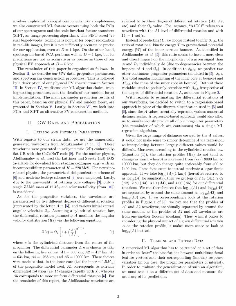
As mentioned in [5], most of the information about the rota-tional parameters of a CCSN is encoded in its pressure-drivenbounce signal, which manifests itself as a large-bandwidthblob in the spectrogram domain. In particular, if we increaseΩc while holding A constant as shown in Figure 4, we findthe following trends in our spectrogram:• The pressure-driven bounce blob becomes more promi-

nent relative to the post-bounce convection blobs.• The bounce blob’s frequency bandwidth decreases.• The bounce blob’s central frequency decreases.• The bounce blob becomes slightly wider (in the time

domain), especially for extreme values of Ωc.From a signal-processing perspective, the second and third

bullet points agree with the fourth: since the bounce takesslightly longer as Ωc and βic,b increase, it can be approximatedby a lower-frequency sinusoidal wave. Physically, this meansthat CCSNe with larger angular velocities have a slightlylonger bounce, which makes sense given their larger angularmomenta. We can also see that more rapidly rotating CCSNehave a more powerful bounce blob in the spectrogram domain;this is just a consequence of their more strongly time-varyingquadrupole moments during the collapse and bounce phases.

Based on this visual trend, we note that an image-processingalgorithm can key in on the “prominence,” bandwidth, centralfrequency, and duration of the pressure-driven bounce blobin order to infer progenitor parameters. However, no clearcorrelations could be established between the post-bounceconvection blobs’ shapes and any rotation-specific parameters;these blobs simply fluctuated too much in bandwidth, timedelay, time duration, and power without obeying any cleartrend. Furthermore, in practice, the (relatively) low-frequencyconvection blobs were more susceptible to being wiped outby noise in the spectrogram domain.

We therefore only have to consider the bounce portion of theGW signal in the spectrogram domain, as the rest of the signaldoes not clearly encode any physical parameters. While thissomewhat limits the efficacy of our image-processing approach,it also simplifies matters greatly since we only need to focuson the bounce blob.

5

(a) Ωc = 5 rad/s (b) Ωc = 10 rad/s (c) Ωc = 15 rad/s

Figure 4: Strain h+ in the time and spectrogram domains for various different values of Ωc, holding A (the differential rotationparameter) constant at A1. The units for the spectrogram’s power density (represented by the color bar) are in strain2 Hz−1.

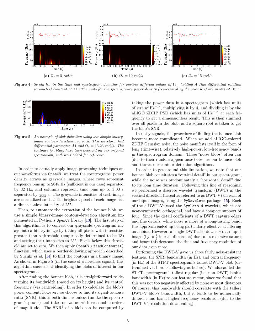
Figure 5: An example of blob detection using our simple binary-image contour-detection approach. This waveform haddifferential parameter A1 and Ωc = 15.25 rad/s. Thecontours (in blue) have been overlaid on our originalspectrogram, with axes added for reference.

In order to actually apply image processing techniques onour waveforms via OpenCV, we treat the spectrograms’ powerdensity arrays as grayscale images, where rows representfrequency bins up to 2048 Hz (sufficient in our case) separatedby 32 Hz, and columns represent time bins up to 3.00 sseparated by 3

4096 s. The grayscale intensities of each imageare normalized so that the brightest pixel of each image hasa dimensionless intensity of 255.Then, to automate the extraction of the bounce blob, we

use a simple binary-image contour-detection algorithm im-plemented in Python’s OpenCV library [13]. The first step ofthis algorithm is to convert our grayscale spectrogram im-age into a binary image by taking all pixels with intensitiesgreater than a threshold (empirically determined to be 13)and setting their intensities to 255. Pixels below this thresh-old are set to zero. We then apply OpenCV’s findContours()function, which uses a border-following approach describedby Suzuki et al. [14] to find the contours in a binary image.As shown in Figure 5 (in the case of a noiseless signal), thisalgorithm succeeds at identifying the blobs of interest in ourspectrograms.After finding the bounce blob, it is straightforward to de-

termine its bandwidth (based on its height) and its centralfrequency (via centroiding). In order to calculate the blob’spower content, however, we choose to find its signal-to-noiseratio (SNR); this is both dimensionless (unlike the spectro-gram’s power) and takes on values with reasonable ordersof magnitude. The SNR2 of a blob can be computed by

taking the power data in a spectrogram (which has unitsof strain2 Hz−1), multiplying it by 4, and dividing it by theaLIGO ZDHP PSD (which has units of Hz−1) at each fre-quency to get a dimensionless result. This is then summedover all pixels in the blob, and a square root is taken to getthe blob’s SNR.In noisy signals, the procedure of finding the bounce blob

becomes more complicated. When we add aLIGO-coloredZDHP Gaussian noise, the noise manifests itself in the form oflong (time-wise), relatively high-power, low-frequency bandsin the spectrogram domain. These “noise blobs” often can(due to their random appearances) obscure our bounce bloband thwart our contour-detection algorithms.In order to get around this limitation, we note that our

bounce blob constitutes a “vertical detail” in our spectrogram,while the noise was predominately a “horizontal detail” dueto its long time duration. Following this line of reasoning,we performed a discrete wavelet transform (DWT) in thevertical direction (hereafter referred to as DWT-V) on each ofour input images, using the PyWavelets package [15]. Eachof these DWT-Vs used the Symlets 4 wavelets, which arenear-symmetric, orthogonal, and have a compact support offour. Since the detail coefficients of a DWT capture edgesand fine details, while noise is more of a long-lasting band,this approach ended up being particularly effective at filteringout noise. However, a single DWT also downsizes an inputimage (by ≈ 1

2 in each dimension) due to its recursive nature,and hence this decreases the time and frequency resolution ofour data even more.

Performing the DWT-V gave us three fairly noise-resistantfeatures: the SNR, bandwidth (in Hz), and central frequency(in Hz) of the STFT spectrogram’s tallest DWT-V blob (de-termined via border-following as before). We also added theSTFT spectrogram’s tallest regular (i.e. non-DWT) blob’sbandwidth (in Hz) to our feature vector, since we found thatthis was not too negatively affected by noise at most distances.Of course, this bandwidth should correlate with the tallestDWT-V blob’s bandwidth, but it tends to be numericallydifferent and has a higher frequency resolution (due to theDWT-V’s resolution downscaling).

6

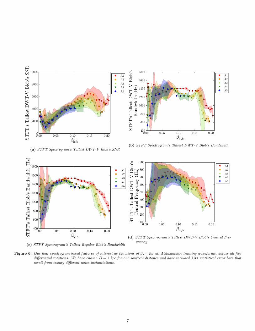
(a) STFT Spectrogram’s Tallest DWT-V Blob’s SNR(b) STFT Spectrogram’s Tallest DWT-V Blob’s Bandwidth

(c) STFT Spectrogram’s Tallest Regular Blob’s Bandwidth

(d) STFT Spectrogram’s Tallest DWT-V Blob’s Central Fre-quency

Figure 6: Our four spectrogram-based features of interest as functions of βic,b for all Abdikamalov training waveforms, across all fivedifferential rotations. We have chosen D = 1 kpc for our source’s distance and have included ±3σ statistical error bars thatresult from twenty different noise instantiations.

7

The relations between our four spectrogram-based featuresand βic,b are shown in Figure 6. To include the effects ofnoise in this figure, we use twenty separate instantiations ofaLIGO noise for each waveform in the catalog, where eachwaveform is scaled to D = 1 kpc before adding noise. Wethen graph the mean feature values for each waveform withpoints, and use translucent shading for ±3σ statistical errorbars to show the expected spread due to noise. While onecould argue that symmetric, ±3σ intervals are a bit excessive,they do reasonably indicate the kinds of variation we couldexpect simply due to randomness in the aLIGO measurementprocedure.

As Figure 6 demonstrates, our spectrogram-based featuresseem to depend mostly on βic,b, with significantly less depen-dence on the differential rotation. We also see the aforemen-tioned visual trends in our figure. For instance, the tallestDWT-V blob’s SNR tends to increase with βic,b before mostlyflattening out. In the central frequency graph and the twobandwidth graphs, we see a decreasing trend for βic,b & 0.05as mentioned earlier. On the other hand, for βic,b . 0.05, thebandwidth and central frequency increase with βic,b as theblob is starting to fade into view on our spectrogram. Unfor-tunately, for very low values of βic,b, there is no clear trend inany of these visual features since the bounce blob is too dimto be seen. This is another important drawback of taking animage-processing approach to parameter estimation.

II. Strain-Based Features

Since the four aforementioned spectrogram-based features arenot sufficient for an ML algorithm – especially since only oneof them changes monotonically with βic,b – we also includethree additional features that can be determined directly fromthe strain h+(t) without image processing.For example, we can directly use the strain data to get a

sense of “how much” of our entire waveform’s signal is due to(say) convection, and how much is due to the pressure-drivenbounce. This can be quantized by looking at the signal-to-noise ratio (SNR) integrand of our training waveforms overvarious bands in frequency space, since we expect the pressure-driven bounce signal to occupy higher frequencies than theconvection signal. The integrand of interest in this case isgiven by:

SNRSI = 4

∣∣∣h(f)∣∣∣2

Sh(f), (2)

where h(f) is the Fourier transform of the strain h(t), Sh(f)is the one-sided aLIGO ZDHP spectral noise density, andSNRSI stands for “SNR Squared’s Integrand.” In Figure 7, wehave plotted this integrand as a function of frequency for thenoiseless A1O07 (Ωc = 7 rad/s), A1O12.5 (Ωc = 12.5 rad/s),and A1O15.5 (Ωc = 15.5 rad/s) waveforms. We can clearlysee the emergence of the pressure-driven bounce in the 400+Hz band of Figure 7b. Moreover, as we increase Ωc, the peakcorresponding to the pressure-driven bounce shifts towardslower frequencies. This agrees with what we had seen in the

Figure 8: SNR in various frequency bands for noiseless A1 wave-forms from the Abdikamalov catalog, as a function ofΩc. We set D = 1 kpc for these waveforms.

spectrogram domain: the bounce blob’s central frequencytends to decrease as we increase Ωc (holding A constant).In order to quantify the amount of signal from each con-

tributing source (e.g. pressure-driven bounce vs. convection)in each waveform, we split up our frequency domain intothree bands: a 60-200 Hz band for low-frequency neutrinoconvection content; a 200-400 Hz band for higher-frequencyprompt convection; and a 400-1100 Hz band that predom-inantly captures the pressure-driven bounce (although thebounce sometimes shifted towards frequencies less than 400Hz). Higher-frequency content was ignored as it was mostlysuppressed by the aLIGO noise PSD. We then performedRiemann integration on the SNRSI to calculate the SNR2

in each of the three bands, and took the square root of thisresult to get a total of three SNR features.

The results of this integration are shown in Figure 8, wherewe plot each SNR as a function of Ωc for noiseless A1 wave-forms, assuming a 1 kpc distance from the source. Thepressure-driven bounce’s gradual emergence can be seen inthe almost monotonic increase of the 400-1100 Hz SNR fromΩc = 4 rad/s to Ωc = 12 rad/s. At higher values of Ωc,the bounce signal starts to move into the 200-400 Hz bandinstead. We can also see a general (but less clear) increasein the 200-400 Hz SNR as a function of Ωc. Physically, thismight seem to indicate an increase in prompt convection withΩc, but it is more likely that some of the bounce signal iscreeping into the 200-400 Hz band.The 60-200 Hz band, on the other hand, exhibits very

unclear behavior as a function of Ωc. It’s possible that thisis just the physical truth, i.e. that the neutrino convectionsignal is simply too stochastic (in both the time and frequencydomains) for us to extract any meaningful conclusions aboutprogenitor parameters. On the other hand, it is likely that theAbdikamalov simulations did not run long enough to resolve

8

(a) Ωc = 7 rad/s (b) Ωc = 12.5 rad/s (c) Ωc = 15.5 rad/s

Figure 7: The SNRSI (defined in (2)) as a function of frequency for three A1 (strongly differentially rotating) waveforms from theAbdikamalov catalog. We set D = 1 kpc. Note that we have not added any noise to the underlying waveforms.

all of the post-bounce convection, and so we simply haveincomplete convection data.Despite these concerns, the 200-400 Hz and 400-1100 Hz

SNRs are still useful features to use for categorizing our wave-forms. Moreover, the SNR integrals tend to be very robust tonoise. While the individual integrands (at specific frequencies)might be less robust to random, Gaussian, aLIGO-colorednoise, the effects of noise tend to “cancel out” reasonably wellwhen it comes to measuring the integral as a whole.

As our third and final strain-based feature, we looked intomeasuring a proxy for the bounce duration. As mentionedin the previous subsection, the bounce blob became slightlywider in the time domain, especially for large values of βic,b.However, we cannot easily measure the bounce blob’s durationvia the STFT spectrogram due to its limited time resolution,and so we instead use time-domain methods. In order totackle noise, we first apply a 20th-order low-pass Butterworthfilter to our signal, with a passband frequency of 1530 Hzand a stopband frequency of 1800 Hz. This gets rid of someof the very high-frequency random noise in our strain dataand helps minimize the number of “false peaks” in our strainsignal. Next, we apply a 3rd-order high-pass Butterworthfilter with a passband frequency of ∼ 82 Hz and a stopbandfrequency of ∼ 20.5 Hz. This removes most low-frequency,large oscillations from our strain signal, and helps ensure that– at points where no CCSN signal was present – the filteredh(t) was close to zero.After applying these two filters, we determined the most

negative minimum in the strain, and assumed it was thenegative trough that occurs at bounce time in CCSN signals.We then found the positive maximum right before this trough,and assumed that it was the positive peak in h(t) right beforebounce. These points can be seen in Figure 9. As a proxyfor the bounce duration, we then take the time differencebetween these two extrema. In general, this algorithm workswell for finding the bounce duration for βic,b & 0.025; forlower values, it often keys in on unrelated convection extremasince the bounce signal is too weak.In Figure 10, we plot our three strain-based features of

interest as functions of βic,b for all differential rotations. Once

Figure 9: Filtering and extrema-finding on a noisy strain signal(D = 1 kpc) for the A1O04 waveform.

again, we scale our waveforms to D = 1 kpc, use twentyinstantiations of aLIGO noise per waveform, and include ±3σstatistical error bars.It is worth noting that, in Figure 10b, for high values of

βic,b (i.e. βic,b ≥ 0.10), there are discrepancies in the 400-1100 Hz SNR for different differential rotations (holding βic,bconstant). This finding agrees with Figure 9 of [5], whereAbdikamalov et al. noticed that rapidly spinning models(with βic,b ∼ 0.10) had significant differences in waveformmorphology with different values of A. Specifically, while thelength of the bounce spike (in the time domain) remained thesame for all values of A, more strongly differentially rotatingmodels had more extreme strain values during the bouncephase. In our case, this directly corresponds to different valuesfor the 400-1100 Hz SNR (Figure 10b) for βic,b ≥ 0.10, as wellas slight differences in the tallest DWT-V blob’s SNR (Figure6a) for the same range of βic,b values. These deviations areuseful in helping us estimate the degree of differential rotationA for rapidly rotating cores (βic,b ≥ 0.10).

9

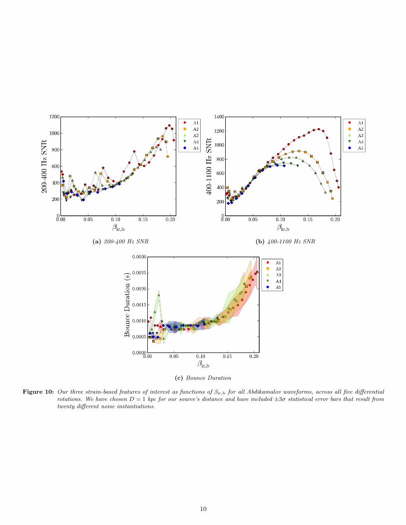
(a) 200-400 Hz SNR (b) 400-1100 Hz SNR

(c) Bounce Duration

Figure 10: Our three strain-based features of interest as functions of βic,b for all Abdikamalov waveforms, across all five differentialrotations. We have chosen D = 1 kpc for our source’s distance and have included ±3σ statistical error bars that result fromtwenty different noise instantiations.

10

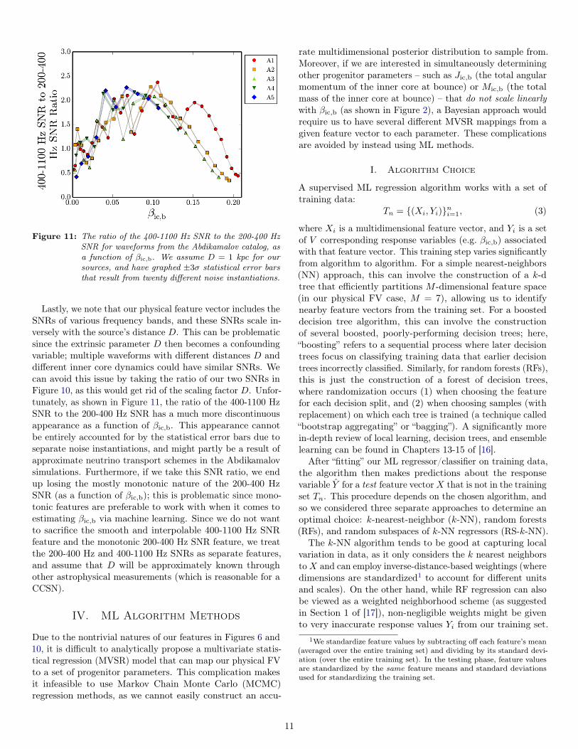
Figure 11: The ratio of the 400-1100 Hz SNR to the 200-400 HzSNR for waveforms from the Abdikamalov catalog, asa function of βic,b. We assume D = 1 kpc for oursources, and have graphed ±3σ statistical error barsthat result from twenty different noise instantiations.

Lastly, we note that our physical feature vector includes theSNRs of various frequency bands, and these SNRs scale in-versely with the source’s distance D. This can be problematicsince the extrinsic parameter D then becomes a confoundingvariable; multiple waveforms with different distances D anddifferent inner core dynamics could have similar SNRs. Wecan avoid this issue by taking the ratio of our two SNRs inFigure 10, as this would get rid of the scaling factor D. Unfor-tunately, as shown in Figure 11, the ratio of the 400-1100 HzSNR to the 200-400 Hz SNR has a much more discontinuousappearance as a function of βic,b. This appearance cannotbe entirely accounted for by the statistical error bars due toseparate noise instantiations, and might partly be a result ofapproximate neutrino transport schemes in the Abdikamalovsimulations. Furthermore, if we take this SNR ratio, we endup losing the mostly monotonic nature of the 200-400 HzSNR (as a function of βic,b); this is problematic since mono-tonic features are preferable to work with when it comes toestimating βic,b via machine learning. Since we do not wantto sacrifice the smooth and interpolable 400-1100 Hz SNRfeature and the monotonic 200-400 Hz SNR feature, we treatthe 200-400 Hz and 400-1100 Hz SNRs as separate features,and assume that D will be approximately known throughother astrophysical measurements (which is reasonable for aCCSN).

IV. ML Algorithm Methods

Due to the nontrivial natures of our features in Figures 6 and10, it is difficult to analytically propose a multivariate statis-tical regression (MVSR) model that can map our physical FVto a set of progenitor parameters. This complication makesit infeasible to use Markov Chain Monte Carlo (MCMC)regression methods, as we cannot easily construct an accu-

rate multidimensional posterior distribution to sample from.Moreover, if we are interested in simultaneously determiningother progenitor parameters – such as Jic,b (the total angularmomentum of the inner core at bounce) or Mic,b (the totalmass of the inner core at bounce) – that do not scale linearlywith βic,b (as shown in Figure 2), a Bayesian approach wouldrequire us to have several different MVSR mappings from agiven feature vector to each parameter. These complicationsare avoided by instead using ML methods.

I. Algorithm Choice

A supervised ML regression algorithm works with a set oftraining data:

Tn = (Xi, Yi)ni=1, (3)

where Xi is a multidimensional feature vector, and Yi is a setof V corresponding response variables (e.g. βic,b) associatedwith that feature vector. This training step varies significantlyfrom algorithm to algorithm. For a simple nearest-neighbors(NN) approach, this can involve the construction of a k-dtree that efficiently partitions M -dimensional feature space(in our physical FV case, M = 7), allowing us to identifynearby feature vectors from the training set. For a boosteddecision tree algorithm, this can involve the constructionof several boosted, poorly-performing decision trees; here,“boosting” refers to a sequential process where later decisiontrees focus on classifying training data that earlier decisiontrees incorrectly classified. Similarly, for random forests (RFs),this is just the construction of a forest of decision trees,where randomization occurs (1) when choosing the featurefor each decision split, and (2) when choosing samples (withreplacement) on which each tree is trained (a technique called“bootstrap aggregating” or “bagging”). A significantly morein-depth review of local learning, decision trees, and ensemblelearning can be found in Chapters 13-15 of [16].

After “fitting” our ML regressor/classifier on training data,the algorithm then makes predictions about the responsevariable Y for a test feature vectorX that is not in the trainingset Tn. This procedure depends on the chosen algorithm, andso we considered three separate approaches to determine anoptimal choice: k-nearest-neighbor (k-NN), random forests(RFs), and random subspaces of k-NN regressors (RS-k-NN).

The k-NN algorithm tends to be good at capturing localvariation in data, as it only considers the k nearest neighborstoX and can employ inverse-distance-based weightings (wheredimensions are standardized1 to account for different unitsand scales). On the other hand, while RF regression can alsobe viewed as a weighted neighborhood scheme (as suggestedin Section 1 of [17]), non-negligible weights might be givento very inaccurate response values Yi from our training set.

1We standardize feature values by subtracting off each feature’s mean(averaged over the entire training set) and dividing by its standard devi-ation (over the entire training set). In the testing phase, feature valuesare standardized by the same feature means and standard deviationsused for standardizing the training set.

11

This renders the RF approach slightly more susceptible toinaccurate response values.

At the same time, the RF approach has two main benefitsover k-NN: it can account for correlations between responsevariables, as well as unbalanced training sets. With regardsto correlations in predicting a set of V variables, k-NN simplytreats the V response variables independently. Specifically, itjust finds the closest k feature vectors to X in the training setand weights their response variables by Euclidean distance;thus, factoring out noise, we expect the same prediction re-sults regardless of whether k-NN separately or simultaneouslydetermined the V variables. Even if the popular Mahalanobisdistance metric is applied, only correlations between featurevector components can be accounted for, not those betweenresponse variables. On the other hand, when random forestsdeal with V > 1 response variables, they compute the av-erage reduction in their quality criterion (e.g. mean squareerror) across all V outputs to arrive at a splitting criterionfor each node. If the output values for a given feature vectorare correlated, looking at the average reduction in a singleforest (instead of building independent forests) lets us takeinto account these correlations. This is advantageous for ussince we know that Mic,b, Jic,b, and βic,b are correlated, andall three of these are dependent on the rotation profile andhence log10(A).

Moreover, random forests have a more appropriate methodof dealing with the issue of unbalanced classes. This occurswhen the training data is (1) split unequally among the classesof interest, and (2) we have reason to believe that this splittingmethod is not representative of how real data will actuallybe partitioned. In the case of the Abdikamalov trainingcatalog, we have a relative abundance of strongly differentiallyrotating models (e.g. A1) and a relative dearth of uniformlydifferentially rotating models (e.g. A5). This is problematicsince it would make our algorithm relatively poor at inferringlog10(A) from uniformly rotating CCSN signals.

This discrepancy in waveform numbers occurs since, whilethe training models for each differential rotation are alwaysseparated by ∆Ωc = 0.5 rad/s, models with low to moderatedifferential rotation tend to not collapse at large values of Ωc.Physically, this occurs since – with higher Ωc – uniformly andmildly differentially rotating models (e.g. A3-A5) have a largeramount of centrifugal support at the start of a simulation, andhence do not collapse [5]. But this does not necessarily meanthat CCSNe from strongly differentially rotating progenitorswill occur more frequently in nature, since stellar evolutionmight not favor such progenitors.

For the purposes of our ML approach, we want to assumea uniform prior and consider all differential rotations equallylikely. From the random forest point of view, this is easilyaccomplished by re-weighting the priors used for each node’ssplitting criterion. In our case, we re-weight all of the wave-forms of a given differential rotation A by αmin/α, whereα is the number of training waveforms with differential ro-tation A and αmin is the lowest value of α. On the otherhand, k-NN cannot really tweak any priors; to account for

unbalanced classes, one must either undersample the majorityclass or oversample the minority class [16]. Undersamplingis infeasible since there are three times more A1 waveformsthan A5 ones. Oversampling, on the other hand, involvessynthesizing new feature vectors via the Synthetic Minor-ity Oversampling Technique (SMOTE) [18], which randomlyinterpolates between the nearest same-class neighbors to agiven waveform. While it is already problematic to deal withunphysical, synthesized data, SMOTE also has the drawbackof only oversampling by integer factors; thus, true equalitycannot be achieved.To decide between RF and k-NN for our physical FV ap-

proach, we empirically evaluate the aforementioned trade-offswith the Python ML library scikit-learn [19]. HoldingD constant at 5 kpc, we find that k-NN2 is noticeably lessprecise than balanced RF3 in terms of the width of its ±2σprediction intervals for most progenitor parameters. Qualita-tive comparisons between the βic,b predictions of these twomethodologies can be found in Appendix A. Due to RF’s ro-bustness to noise and aforementioned theoretical advantages,we therefore focus solely on RF-related results in Section V.

Lastly, we briefly consider the RS-k-NN approach since –while a single k-NN regressor might do reasonably well – NNalgorithms tend to perform relatively poorly with very-high-dimensional data due to the so-called “curse of dimensionality”[16]. Thus, we apply the random subspace (RS) ensemblelearning approach with 150 4-NN regressors trained on 40randomly chosen training samples (with D = 5 kpc) andthree randomly chosen features each. As shown in Figure 22of Appendix A, however, the RS-4-NN method actually tendsto undershoot more often at high βic,b values compared tothe usual 4-NN approach, and is overall slightly less accurate.This seems to suggest that the curse of dimensionality is not avery significant issue for us. To the contrary, we need all sevenfeature vector dimensions to properly distinguish betweentraining waveforms at all βic,b values, and randomness canoften exclude useful monotonic features.

II. RF Algorithm Implementation

To construct our regression algorithms, we use theRandomForestRegressor module from scikit-learn. Forour forest parameters, we grow 150 decision trees (as RF doesnot overfit) with bootstrap aggregation (“bagging”), max-imal depth (i.e. nodes expanded until all leaves are pure,where purity is measured by the mean-square-error (MSE)quality criterion), and consider all features at each decisionsplit. To account for correlations, we simultaneously pre-dict all four progenitor parameters – βic,b, Jic,b, Mic,b, andlog10(A) – with a single random forest. Lastly, we re-weightour training waveforms’ priors to account for unbalanced dif-ferential rotation classes, using the aforementioned procedure

2With an optimal case of k = 4, inverse-distance-based weightings,and 3-nearest-neighbors SMOTE-balancing for log10(A) regression

3Implementation details for RF are outlined in the following subsec-tion.

12

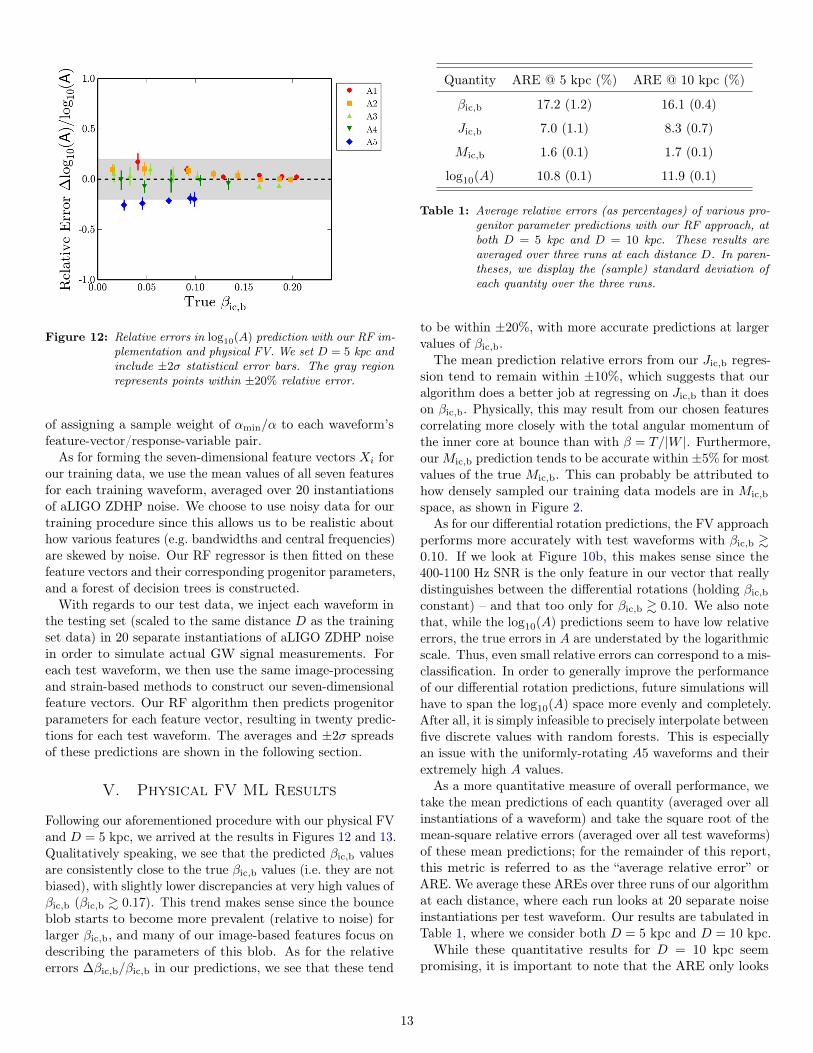
Figure 12: Relative errors in log10(A) prediction with our RF im-plementation and physical FV. We set D = 5 kpc andinclude ±2σ statistical error bars. The gray regionrepresents points within ±20% relative error.

of assigning a sample weight of αmin/α to each waveform’sfeature-vector/response-variable pair.

As for forming the seven-dimensional feature vectors Xi forour training data, we use the mean values of all seven featuresfor each training waveform, averaged over 20 instantiationsof aLIGO ZDHP noise. We choose to use noisy data for ourtraining procedure since this allows us to be realistic abouthow various features (e.g. bandwidths and central frequencies)are skewed by noise. Our RF regressor is then fitted on thesefeature vectors and their corresponding progenitor parameters,and a forest of decision trees is constructed.

With regards to our test data, we inject each waveform inthe testing set (scaled to the same distance D as the trainingset data) in 20 separate instantiations of aLIGO ZDHP noisein order to simulate actual GW signal measurements. Foreach test waveform, we then use the same image-processingand strain-based methods to construct our seven-dimensionalfeature vectors. Our RF algorithm then predicts progenitorparameters for each feature vector, resulting in twenty predic-tions for each test waveform. The averages and ±2σ spreadsof these predictions are shown in the following section.

V. Physical FV ML Results

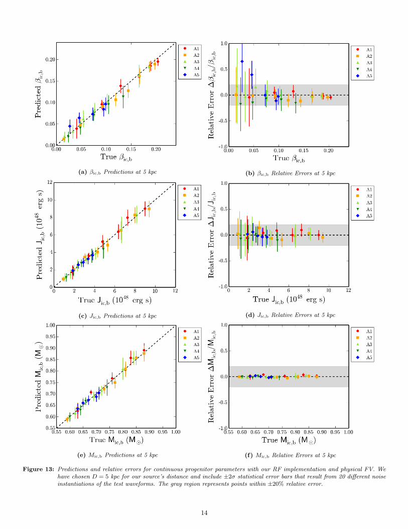
Following our aforementioned procedure with our physical FVand D = 5 kpc, we arrived at the results in Figures 12 and 13.Qualitatively speaking, we see that the predicted βic,b valuesare consistently close to the true βic,b values (i.e. they are notbiased), with slightly lower discrepancies at very high values ofβic,b (βic,b & 0.17). This trend makes sense since the bounceblob starts to become more prevalent (relative to noise) forlarger βic,b, and many of our image-based features focus ondescribing the parameters of this blob. As for the relativeerrors ∆βic,b/βic,b in our predictions, we see that these tend

Quantity ARE @ 5 kpc (%) ARE @ 10 kpc (%)

βic,b 17.2 (1.2) 16.1 (0.4)

Jic,b 7.0 (1.1) 8.3 (0.7)

Mic,b 1.6 (0.1) 1.7 (0.1)

log10(A) 10.8 (0.1) 11.9 (0.1)

Table 1: Average relative errors (as percentages) of various pro-genitor parameter predictions with our RF approach, atboth D = 5 kpc and D = 10 kpc. These results areaveraged over three runs at each distance D. In paren-theses, we display the (sample) standard deviation ofeach quantity over the three runs.

to be within ±20%, with more accurate predictions at largervalues of βic,b.

The mean prediction relative errors from our Jic,b regres-sion tend to remain within ±10%, which suggests that ouralgorithm does a better job at regressing on Jic,b than it doeson βic,b. Physically, this may result from our chosen featurescorrelating more closely with the total angular momentum ofthe inner core at bounce than with β = T/|W |. Furthermore,ourMic,b prediction tends to be accurate within ±5% for mostvalues of the true Mic,b. This can probably be attributed tohow densely sampled our training data models are in Mic,b

space, as shown in Figure 2.As for our differential rotation predictions, the FV approach

performs more accurately with test waveforms with βic,b &0.10. If we look at Figure 10b, this makes sense since the400-1100 Hz SNR is the only feature in our vector that reallydistinguishes between the differential rotations (holding βic,bconstant) – and that too only for βic,b & 0.10. We also notethat, while the log10(A) predictions seem to have low relativeerrors, the true errors in A are understated by the logarithmicscale. Thus, even small relative errors can correspond to a mis-classification. In order to generally improve the performanceof our differential rotation predictions, future simulations willhave to span the log10(A) space more evenly and completely.After all, it is simply infeasible to precisely interpolate betweenfive discrete values with random forests. This is especiallyan issue with the uniformly-rotating A5 waveforms and theirextremely high A values.

As a more quantitative measure of overall performance, wetake the mean predictions of each quantity (averaged over allinstantiations of a waveform) and take the square root of themean-square relative errors (averaged over all test waveforms)of these mean predictions; for the remainder of this report,this metric is referred to as the “average relative error” orARE. We average these AREs over three runs of our algorithmat each distance, where each run looks at 20 separate noiseinstantiations per test waveform. Our results are tabulated inTable 1, where we consider both D = 5 kpc and D = 10 kpc.

While these quantitative results for D = 10 kpc seempromising, it is important to note that the ARE only looks

13

(a) βic,b Predictions at 5 kpc (b) βic,b Relative Errors at 5 kpc

(c) Jic,b Predictions at 5 kpc (d) Jic,b Relative Errors at 5 kpc

(e) Mic,b Predictions at 5 kpc (f) Mic,b Relative Errors at 5 kpc

Figure 13: Predictions and relative errors for continuous progenitor parameters with our RF implementation and physical FV. Wehave chosen D = 5 kpc for our source’s distance and include ±2σ statistical error bars that result from 20 different noiseinstantiations of the test waveforms. The gray region represents points within ±20% relative error.

14

Figure 14: Predicted βic,b values (with ±2σ statistical error bars)for our RF implementation with physical FVs at D =10 kpc.

at the relative error of the mean predicted value (averagedover 20 noise instantiations). In other words, it does notgive us a sense of the spread of our predicted values dueto different noise instantiations, and this spread tends toincrease with D. This increase can be seen by looking atFigure 14, where we set D = 10 kpc and predict βic,b. Atthis distance, our predictions retain their levels of accuracy(on average), but are only precise in the case of rapidly-rotating models (βic,b & 0.17), where the bounce blob is moreprominent and where some trends (e.g. changes in the bounceduration) become more extreme. Statistically, the impreciseperformance of our algorithm at 10 kpc makes sense sincemany of the trends in our feature vector data can becomeobscured by detector noise as our signal gets weaker. Otherprogenitor parameter predictions show similar decreases inaccuracy and increases in statistical error when we increaseD to 10 kpc.

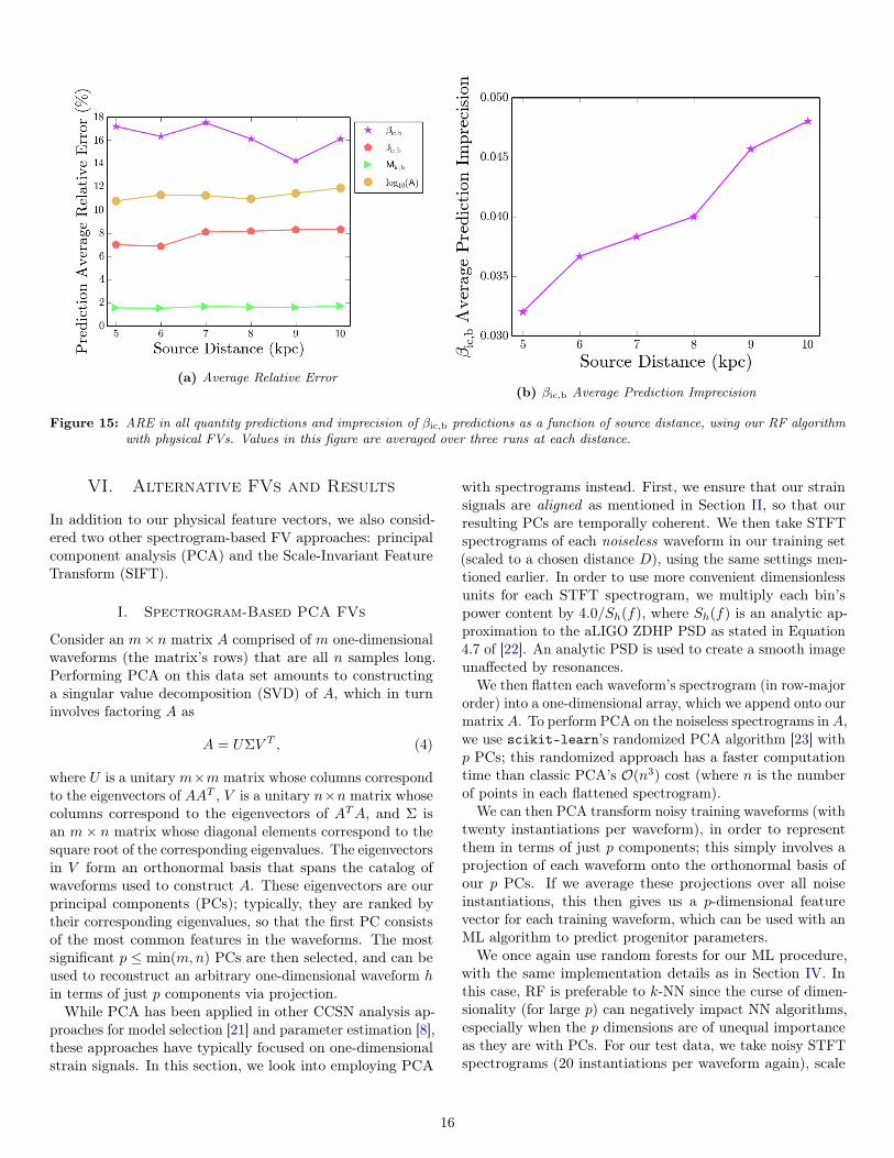
To determine how our algorithm’s performance varies withD, we graphed our predictions’ AREs as a function of D forsix source distances from 5 to 10 kpc. We also graph ouraverage βic,b prediction imprecision as a function of D; thislatter quantity is measured as the average full width of our±2σ prediction intervals for βic,b over all 31 test waveforms.Our results are shown in Figure 15; for each distance, we haveaveraged results over three runs of our algorithm.Figure 15a shows that there is no significant trend in the

ARE of most of our quantities’ predictions as a function ofsource distance D. While this seems counter-intuitive, it isimportant to remember that our algorithm uses a differentset of training data for each distance D, in order to accountfor how feature trends appear different with weaker signals(e.g. the SNRs inversely scale with D). Since our chosenphysical features still remain mostly interpolable in our train-ing data, it therefore makes sense that our noisy test datawould yield accurate results on average, even as D increases.However, the spreading effect of noise becomes clear in Figure

Feature Importance

STFT’s Tallest DWT-V

Blob’s SNR0.069

STFT’s Tallest DWT-V

Blob’s Bandwidth0.033

STFT’s Tallest Regular

Blob’s Bandwidth0.063

STFT’s Tallest DWT-V

Blob’s Central Frequency0.030

200-400 Hz SNR 0.538

400-1100 Hz SNR 0.109

Bounce Duration 0.157

Table 2: Feature importances computed by scikit-learn for ourRF algorithm. These values are based on training datawith D = 5 kpc, and are only meant to give a qualita-tive idea of importances; due to randomness, they willfluctuate slightly from forest to forest.

15b, as our average βic,b imprecision worsens from ∼ 0.03 to∼ 0.05; similar trends apply to the prediction imprecisions ofother progenitor parameters.

As a final point of interest, we record in Table 2 the featureimportances produced by scikit-learn for our RF algorithmwith D = 5 kpc. A feature’s “importance” in this sense isdirectly related to the decision trees constructed for a setof training data. One can imagine treating the depth (ina tree) of a feature used as a decision node as a measureof the relative importance of that feature when it comes topredicting the response variable; features near the top of atree tend to contribute to the final prediction result for a muchlarger fraction of test data. Following this line of reasoning,a feature’s importance in scikit-learn is defined as theexpected fraction of samples whose classifications are aidedby that feature [20]. These importance values are normalizedso as to sum to unity.

Table 2 suggests that, in determining progenitor parametersvia random forests, the 200-400 Hz SNR, 400-1100 Hz SNR,and bounce duration play the most important roles when itcomes to decision splits. This can be understood by lookingat the relatively non-fluctuating relationships between thesefeatures and βic,b in Figure 10. Moreover, since the 200-400Hz SNR has a mostly monotonic dependence on βic,b, it makessense that its importance would be particularly high; this alsoexplains the relatively high importance of the monotonicallyincreasing bounce duration. Spectrogram-based (i.e. bounce-blob-related) features, on the other hand, tend to have lowerfeature importances due to their fluctuations and mostlynonmonotonic behaviors.

15

(a) Average Relative Error(b) βic,b Average Prediction Imprecision

Figure 15: ARE in all quantity predictions and imprecision of βic,b predictions as a function of source distance, using our RF algorithmwith physical FVs. Values in this figure are averaged over three runs at each distance.

VI. Alternative FVs and Results

In addition to our physical feature vectors, we also consid-ered two other spectrogram-based FV approaches: principalcomponent analysis (PCA) and the Scale-Invariant FeatureTransform (SIFT).

I. Spectrogram-Based PCA FVs

Consider an m×n matrix A comprised of m one-dimensionalwaveforms (the matrix’s rows) that are all n samples long.Performing PCA on this data set amounts to constructinga singular value decomposition (SVD) of A, which in turninvolves factoring A as

A = UΣV T , (4)

where U is a unitary m×m matrix whose columns correspondto the eigenvectors of AAT , V is a unitary n×n matrix whosecolumns correspond to the eigenvectors of ATA, and Σ isan m× n matrix whose diagonal elements correspond to thesquare root of the corresponding eigenvalues. The eigenvectorsin V form an orthonormal basis that spans the catalog ofwaveforms used to construct A. These eigenvectors are ourprincipal components (PCs); typically, they are ranked bytheir corresponding eigenvalues, so that the first PC consistsof the most common features in the waveforms. The mostsignificant p ≤ min(m,n) PCs are then selected, and can beused to reconstruct an arbitrary one-dimensional waveform hin terms of just p components via projection.While PCA has been applied in other CCSN analysis ap-

proaches for model selection [21] and parameter estimation [8],these approaches have typically focused on one-dimensionalstrain signals. In this section, we look into employing PCA

with spectrograms instead. First, we ensure that our strainsignals are aligned as mentioned in Section II, so that ourresulting PCs are temporally coherent. We then take STFTspectrograms of each noiseless waveform in our training set(scaled to a chosen distance D), using the same settings men-tioned earlier. In order to use more convenient dimensionlessunits for each STFT spectrogram, we multiply each bin’spower content by 4.0/Sh(f), where Sh(f) is an analytic ap-proximation to the aLIGO ZDHP PSD as stated in Equation4.7 of [22]. An analytic PSD is used to create a smooth imageunaffected by resonances.

We then flatten each waveform’s spectrogram (in row-majororder) into a one-dimensional array, which we append onto ourmatrix A. To perform PCA on the noiseless spectrograms in A,we use scikit-learn’s randomized PCA algorithm [23] withp PCs; this randomized approach has a faster computationtime than classic PCA’s O(n3) cost (where n is the numberof points in each flattened spectrogram).

We can then PCA transform noisy training waveforms (withtwenty instantiations per waveform), in order to representthem in terms of just p components; this simply involves aprojection of each waveform onto the orthonormal basis ofour p PCs. If we average these projections over all noiseinstantiations, this then gives us a p-dimensional featurevector for each training waveform, which can be used with anML algorithm to predict progenitor parameters.We once again use random forests for our ML procedure,

with the same implementation details as in Section IV. Inthis case, RF is preferable to k-NN since the curse of dimen-sionality (for large p) can negatively impact NN algorithms,especially when the p dimensions are of unequal importanceas they are with PCs. For our test data, we take noisy STFTspectrograms (20 instantiations per waveform again), scale

16

(a) PCA-Based 50-Component FV at 1 kpc (b) Physical 7-Dimensional FV at 1 kpc

(c) PCA-Based 50-Component FV at 5 kpc (d) Physical 7-Dimensional FV at 5 kpc

Figure 16: Predicted βic,b vs true βic,b, using both PCA-based FVs and physical FVs. We include results for both D = 1 kpc and D = 5kpc.

17

Figure 17: The tiling of time-frequency-Q space in a QT spec-trogram. The tiles are spaced linearly in time andlogarithmically in frequency and Q. Figure adaptedfrom [25].

them by 4.0/Sh(f), flatten them into one dimension, andPCA transform to get a p-dimensional feature vector. Ourtest waveforms must also be aligned as before, since PCArelies on temporal coherence (in our case, a known bouncetime).From a qualitative point of view, we found that more PC

components generally led to a better performance in predictingβic,b. In the end, we decided on p = 50 since we found thatour random forest’s feature importances were on the order of10−4 when additional PCs were added.

Our results for βic,b prediction with this ML procedure atD = 1 kpc and D = 5 kpc are shown in Figure 16, placedside-by-side with the results from our physical FV approach(similar results qualitatively apply for other progenitor pa-rameters). We can see that, at D = 1 kpc, the PCA approachactually performs better in terms of both precision and accu-racy. However, when we increase D to 5 kpc, PCA becomesless accurate and significantly less precise. This poor perfor-mance might result from PCA keying in on noise or otherfeatures (e.g. convection blobs) that are not strongly corre-lated with our chosen progenitor parameters. It might alsoresult from the loss of phase information and suboptimal time-frequency resolutions in spectrograms, which would suggestthat PCA is not entirely suited for spectrogram-only use.

II. SIFT-Based FVs

In the image-processing community, David Lowe’s scale-invariant feature transform (SIFT) is often used in conjunctionwith the “visual bag-of-words” technique to categorize and(later) recognize real-life objects. SIFT uses a difference-of-Gaussians (DoG) pyramid approach at various image scalesto identify the high-contrast parts (e.g. edges or corners) ofan image. Keypoints are identified as scale-space extremaon each of these DoG pyramids. In order to describe thesekeypoints in an orientation-independent manner, the SIFTalgorithm determines the overall orientation of a keypointbased on its pixels’ gradient magnitudes and orientations. Thealgorithm then uses a 128-dimensional keypoint descriptor to

Figure 18: Grayscale QT spectrogram of noisy A1O10 waveformat 1 kpc, with SIFT keypoints overlaid as coloredcircles. Axes are logarithmically scaled in frequency(vertical axis) and linearly scaled in time (horizontalaxis). Note that SIFT keys in on the bounce andconvection blobs, but ignores noise blobs.

store information about keypoint pixels’ gradients relative tothis overall orientation. The interested reader should refer toLowe’s original paper [24] for further information on SIFT.Due to the STFT’s poor time resolution, we chose to use

Q-Transform (QT) spectrograms instead of STFT spectro-grams. QT spectrograms differ from conventional STFTspectrograms in that they use non-orthogonal sine-Gaussianfunctions with differing quality factors Q as their basis, asopposed to the orthogonal family of trigonometric functionsused in the STFT. Unlike the STFT, QTs do not have arectangular time-frequency tiling. Instead, they have a highertime resolution at high frequencies, and hence a lower fre-quency resolution at those frequencies (due to the Gaborlimit). For this reason, they tend to be logarithmically tiledin frequency space. This tiling can be seen visually in Figure17.

To bring out convection blobs more (as these tend to be atlow frequencies) and achieve a finer time resolution, we uselogarithmically-spaced frequencies, time bins that are 1/2048 slong, and Q = 0.2 as parameters for astroML’s wavelet_PSDfunction [26]. We then convert our QT spectrogram intostrain2 units by multiplying its powers by 4.0/Sh(f). Toavoid resonances, which can create edges in our spectrogram,we use the analytic expression for Sh(f) as before. Ourspectrogram is then normalized so that the brightest pixelhas an intensity of 255.

18

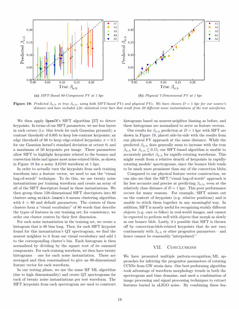
(a) SIFT-Based 80-Component FV at 1 kpc (b) Physical 7-Dimensional FV at 1 kpc

Figure 19: Predicted βic,b vs true βic,b, using both SIFT-based FVs and physical FVs. We have chosen D = 1 kpc for our source’sdistance and have included ±2σ statistical error bars that result from 20 different noise instantiations of the test waveforms.

We then apply OpenCV’s SIFT algorithm [27] to detectkeypoints. In terms of our SIFT parameters, we use four layersin each octave (i.e. blur levels for each Gaussian pyramid); acontrast threshold of 0.005 to keep low-contrast keypoints; anedge threshold of 80 to keep edge-related keypoints; σ = 0.5for our Gaussian kernel’s standard deviation at octave 0; anda maximum of 50 keypoints per image. These parametersallow SIFT to highlight keypoints related to the bounce andconvection blobs and ignore most noise-related blobs, as shownin Figure 18 for a noisy A1O10 waveform at 1 kpc.

In order to actually turn the keypoints from each trainingwaveform into a feature vector, we need to use the “visualbag-of-words” technique. To do this, we use twenty noiseinstantiations per training waveform and create an array ofall of the SIFT descriptors found in these instantiations. Wethen group these 128-dimensional SIFT descriptors into 80clusters using scikit-learn’s k-means clustering algorithmwith k = 80 and default parameters. The centers of theseclusters form a “visual vocabulary” of 80 words that describethe types of features in our training set; for consistency, weorder our cluster centers by their first dimension.

For each noise instantiation in the training set, we create ahistogram that is 80 bins long. Then, for each SIFT keypointfound for this instantiation’s QT spectrogram, we find thenearest neighbor to it from our visual vocabulary and add 1to the corresponding cluster’s bin. Each histogram is thennormalized by dividing by the square root of its summedcomponents. For each training waveform, we then have twentyhistograms – one for each noise instantiation. These areaveraged and then renormalized to give an 80-dimensionalfeature vector for each waveform.In our testing phase, we use the same RF ML algorithm

(due to high dimensionality) and create QT spectrograms foreach of twenty noise instantiations per test waveform. TheSIFT keypoints from each spectrogram are used to construct

histograms based on nearest-neighbor binning as before, andthese histograms are normalized to serve as feature vectors.

Our results for βic,b prediction at D = 1 kpc with SIFT areshown in Figure 19, placed side-by-side with the results fromour physical FV approach at the same distance. While thepredicted βic,b does generally seem to increase with the trueβic,b for βic,b . 0.15, our SIFT-based algorithm is unable toaccurately predict βic,b for rapidly-rotating waveforms. Thismight result from a relative dearth of keypoints in rapidly-rotating models’ spectrograms, since the bounce blob tendsto be much more prominent than any of the convection blobs.Compared to our physical feature vector construction, we

can also see that the SIFT/“visual bag-of-words” approach isfar less accurate and precise at predicting βic,b, even at therelatively close distance of D = 1 kpc. This poor performanceoccurs for many reasons. For example, SIFT misses outon the context of keypoints (e.g. relative positions) and isunable to stitch them together in any meaningful way. Inaddition, SIFT is mostly useful for recognizing starkly differentobjects (e.g. cars vs bikes) in real-world images, and cannotbe expected to perform well with objects that morph as slowlyas our bounce blob. Lastly, it’s possible that SIFT is thrownoff by convection-blob-related keypoints that do not varycontinuously with βic,b or other progenitor parameters – andhence cannot be reasonably “interpolated.”

VII. Conclusions

We have presented multiple pattern-recognition/ML ap-proaches for inferring the progenitor parameters of rotatingCCSNe from GW strain data. Our best-performing algorithmtook advantage of waveform morphology trends in both thespectrogram and time domains, and used a combination ofimage processing and signal processing techniques to extractfeatures buried in aLIGO noise. By combining these fea-

19

tures into a seven-dimensional feature vector and applying arandom forest machine-learning algorithm, we were able tosimultaneously estimate various progenitor parameters for agiven CCSN. Our predictions were accurate on average atboth D = 5 kpc and D = 10 kpc, with average relative errors(for the mean prediction) remaining within ±20% for βic,b,±10% for Jic,b, and ±5% for Mic,b. However, the spread ofour predictions increased noticeably with D; for instance, theaverage full width of ±2σ βic,b prediction intervals increasedfrom ∼ 0.03 at 5 kpc to ∼ 0.05 at 10 kpc.When it comes to determining differential rotations, our

physical FV approach only really performed accurately forβic,b & 0.10. This was the point where slight differencesin waveform morphology started to emerge between modelswith the same βic,b and different differential rotations. Eventhough our procedure performed more accurately with rapidly-rotating models, it was still difficult to interpolate betweenthe five discrete log10(A) values presented in the Abdikamalovcatalog. Future simulations will have to cover log10(A) spacemore evenly and completely if differential rotations are to benumerically predicted from actual signals – especially in thecase of near-uniform rotation.To explore additional image-processing approaches to FV

construction, we also looked into both spectrogram-basedPCA and SIFT. The SIFT-based “visual bag-of-words” tech-nique was found to be very inaccurate and imprecise at D = 1kpc. On the other hand, spectrogram-based PCA workedvery well at D = 1 kpc, although its predictions became no-ticeably less accurate and precise at D = 5 kpc – especially incomparison to our physical FV approach. Thus, it might beworthwhile to use PCA at small source distances D, especiallysince – at these distances – the diminished impact of noisemakes it easier to determine the signal’s arrival time.With regards to future work, the pattern-recognition and

ML algorithms that we’ve described in this paper can bereused to train and test on new rotating core-collapse mod-els as they become available. By training on newer andpresumably more accurate data, our algorithm will becomebetter-equipped at inferring parameters from actual rotatingCCSN GW signals buried in aLIGO noise.

VIII. Acknowledgments

I would like to thank my mentors Alan Weinstein and SarahGossan for their support, discussions, comments, and sug-gested references over the course of my Summer Undergradu-ate Research Fellowship (SURF) at Caltech. I would also liketo acknowledge the NSF for funding my research.

A. Comparisons of ML Algorithms onPhysical FVs

I. RF vs 4-NN

Qualitatively, the 4-NN algorithm is much less precise thanRF in its predictions at both D = 5 kpc and D = 10 kpc, asshown in Figures 20 (5 kpc) and 21 (10 kpc).

(a) RF βic,b Predictions at 5 kpc

(b) 4-NN βic,b Predictions at 5 kpc

Figure 20: Predicted βic,b vs true βic,b, using both 4-NN andRF regressions. We have chosen D = 5 kpc for oursource’s distance and have included ±2σ statisticalerror bars that result from 20 different noise instanti-ations of the test waveforms.

20

(a) RF βic,b Predictions at 10 kpc

(b) 4-NN βic,b Predictions at 10 kpc

Figure 21: The same comparison as in Figure 20, but with D =10 kpc.

II. RS-4-NN vs 4-NN

A qualitative comparison between 4-NN and RS-4-NN isshown in Figure 22, where we predict βic,b with D = 5 kpc.Both algorithms perform similarly, although RS-4-NN tendsto be less accurate at predicting βic,b, especially in the caseof rapidly rotating models (specifically, for βic,b & 0.15).

(a) RS-4-NN βic,b Predictions

(b) 4-NN βic,b Predictions

Figure 22: Predicted βic,b vs true βic,b, using both RS-4-NN and4-NN regressions. We have chosen D = 5 kpc forour source’s distance and have included ±2σ statis-tical error bars that result from 20 different noiseinstantiations of the test waveforms.

21

References

[1] Janka HT, Langanke K, Marek A, Martínez-PinedoG, and Müller B (2007). “Theory of Core-CollapseSupernovae.” Physics Reports, vol. 442, pp. 38-74.doi:10.1016/j.physrep.2007.02.002.

[2] Ott CD (2009). “Topical Review: The Gravitational-Wave Sig-nature of Core-Collapse Supernovae.” Classical and QuantumGravity, vol. 26. doi:10.1088/0264-9381/26/6/063001.

[3] Ott CD et al (2012). “Correlated Gravitational Waveand Neutrino Signals from General-Relativistic Rapidly Ro-tating Iron Core Collapse.” Physical Review D, vol. 86.doi:10.1103/PhysRevD.86.024026.

[4] Adams SM, Kochanek CS, Beacom JF, Vagins MR, andStanek KZ (2013). “Observing the Next Galactic Supernova.”Astrophysical Journal, vol. 778, pp. 164-178. doi:10.1088/0004-637X/778/2/164.

[5] Abdikamalov E, Gossan S, DeMaio AM, and Ott CD (2013).“Measuring the Angular Momentum Distribution in Core-Collapse Supernova Progenitors with Gravitational Waves.”ArXiv e-prints. doi:2013arXiv1311.3678A.

[6] Dimmelmeier H, Ott CD, Marek A, and Janka HT(2008). “Gravitational Wave Burst Signal from Core Col-lapse of Rotating Stars.” Physical Review D, vol. 78.doi:10.1103/PhysRevD.78.064056.

[7] Engels WJ, Frey R, and Ott CD (2014). “Multivariate Re-gression Analysis of Gravitational Waves from Rotating CoreCollapse.” ArXiv e-prints. arXiv:1406.1164.

[8] Edwards MC, Meyer R, and Christensen N (2014). “BayesianParameter Estimation of Core Collapse Supernovae Us-ing Gravitational Wave Simulations.” ArXiv e-prints.arXiv:1407.7549.

[9] CoCoNuT Code. Accessed June 2014. URL.

[10] Woosley SE and Heger A (2007). “Nucleosynthesis and Rem-nants in Massive Stars of Solar Metallicity.” Physics Reports,vol. 442, pp. 269âĂŞ283. doi:10.1016/j.physrep.2007.02.009.

[11] Müller B, Janka HT, and Marek A (2013). “A New Multi-Dimensional General Relativistic Neutrino HydrodynamicsCode of Core-Collapse Supernovae.” The Astrophysical Jour-nal, vol. 766. doi:10.1088/0004-637X/766/1/43.

[12] Advanced LIGO Anticipated Sensitivity Curves. AccessedJune 2014. URL.

[13] OpenCV 3.0.0-dev Documentation. Accessed May 2014. URL.

[14] Suzuki S and Abe K (1985). “Topological Structural Analysisof Digitized Binary Images by Border Following.” ComputerVision, Graphics, and Image Processing, vol. 30, pp. 32âĂŞ46.doi:10.1016/0734-189X(85)90016-7.

[15] PyWavelets – Discrete Wavelet Transform in Python. Ac-cessed June 2014. URL.

[16] Narsky I and Porter FC (2014). “Statistical Analysis Tech-niques in Particle Physics: Fits, Density Estimation andSupervised Learning.” Wiley-VCH, ed. 1. ISBN 978-3-527-41086-6.

[17] Lin Y and Jeon Y (2002). “Random Forests and AdaptiveNearest Neighbors.” Journal of the American Statistical As-sociation. doi:10.1.1.153.9168.

[18] Chawla NV, Bowyer KW Bowyer, Hall LO, and KegelmeyerWP (2002). “SMOTE: Synthetic Minority Over-SamplingTechnique.” Journal of Artificial Intelligence Research, vol.16, pp. 321-357. doi:10.1613/jair.953.

[19] Pedregosa F et al (2011). “Scikit-learn: Machine Learning inPython.” Journal of Machine Learning Research, vol. 12, pp.2825-2830. URL.

[20] Ensemble Methods – scikit-learn 0.15.0 Documentation.Accessed July 2014. URL.

[21] Logue J, Ott CD, Heng IS, Kalmus P, and ScargillJHC (2012). “Inferring Core-Collapse Supernova PhysicsWith Gravitational Waves.” Physical Review D, vol. 86.doi:10.1103/PhysRevD.86.044023.

[22] Ajith P (2011). “Addressing the Spin Question inGravitational-Wave Searches: Waveform Templates for Inspi-ralling Compact Binaries with Nonprecessing Spins.” PhysicalReview D, vol. 84. doi:10.1103/PhysRevD.84.084037.

[23] Halko N, Martinsson P, Shkolnisky Y, and Tygert M (2011).“An Algorithm for the Principal Component Analysis of LargeData Sets.” SIAM Journal on Scientific Computing, vol. 33,pp. 2580-2594. arXiv:1007.5510.

[24] Lowe DG (2004). “Distinctive Image Featuresfrom Scale-Invariant Keypoints.” InternationalJournal of Computer Vision, vol. 60, pp. 91-110.doi:10.1023/B:VISI.0000029664.99615.94.

[25] Chatterji, SK (2004). “The Q Transform Search forGravitational-Wave Bursts With LIGO.” 9th GravitationalWave Data Analysis Workshop. LIGO-G040521-00-Z.

[26] astroML: Machine Learning and Data Mining for Astronomy.Accessed July 2014. URL.

[27] OpenCV SIFT. Accessed June 2014. URL.

22