i fm radio signals - popleteevpopleteev.com/static/pdf/2011/indoor positioning using fm radio... ·...
TRANSCRIPT
PhD Dissertation
April 2011
International Doctorate School in Information and Communication Technologies
DIT - University of Trento
INDOOR POSITIONING USING FM RADIO SIGNALS
Andrei Popleteev
Advisors:
Dr. Oscar Mayora
Dr. Venet Osmani
Prof. Imrich Chlamtac


Abstract
Location based services are becoming an indispensable part of the life.
Wide adoption of the Global Positioning System in mobile devices, com-
bined withWi-Fi and cellular networks, have practically solved the problem
of outdoor localization and opened a new market. This, however, is the
case only for outdoors. There are numerous areas of ubiquitous computing,
which require the knowledge of user position indoors. Awareness of user’s
location is important in such areas as smart environments, assisted daily
living, behaviour analysis studies.
Over the past years, a significant effort has been dedicated to devel-
opment of indoor localization systems. The results vary in characteris-
tics, performance, and cost. Despite the effort, the existing indoor posi-
tioning systems are still limited: they either require expensive infrastruc-
ture (UWB, ultrasound), have limited coverage (Wi-Fi, Bluetooth, RFID,
DECT) or low accuracy (cellular networks). The cost of commercial sys-
tems is prohibitive for their wide adoption (Ubisense).
The main objective of this thesis was to determine the feasibility of
indoor positioning using FM radio signals, generated either by local trans-
mitters or by broadcasting FM stations. The performance of FM localiza-
tion cannot be simply predicted from other technologies, such as Wi-Fi or
GSM, due to significantly lower frequencies (around 100 MHz vs. units of
GHz) leading to differences in signal propagation. Moreover, FM repre-
sents a popular and well-established technology, readily available in many

mobile devices. At the infrastructure side, broadcasting FM stations pro-
vide almost ubiquitous coverage, while short-range FM transmitters are
available license-free from conventional electronics markets.
The results indicate that indoor positioning using broadcasting FM sta-
tions outperforms in terms of accuracy both Wi-Fi and GSM indoor local-
ization systems (for confidence levels up to 90% and in all cases, respec-
tively). Due to the passive nature of the client devices, the system can
be used in sensitive areas where local radio transmission, such as Wi-Fi
or GSM, is prohibited for safety or security reasons. Finally, an FM re-
ceiver has significantly lower power consumption than a Wi-Fi module and
provides 2.6 to 5.5 times longer battery life in localization mode.
Keywords
indoor positioning, FM radio, signal fingerprinting
4
Contents
1 Introduction 1
2 Background 5
2.1 Indoor positioning methods . . . . . . . . . . . . . . . . . . 7
2.1.1 Proximity based . . . . . . . . . . . . . . . . . . . . . 7
2.1.2 Direction based . . . . . . . . . . . . . . . . . . . . . 8
2.1.3 Time based (multilateration) . . . . . . . . . . . . . . 9
2.1.4 Signal property based . . . . . . . . . . . . . . . . . . 10
2.1.5 Summary . . . . . . . . . . . . . . . . . . . . . . . . . 14
2.2 State of the art wireless indoor positioning systems . . . . . 16
2.2.1 Wi-Fi-based systems . . . . . . . . . . . . . . . . . . . 16
2.2.2 Cellular network-based systems . . . . . . . . . . . . . 18
2.2.3 FM radio-based systems . . . . . . . . . . . . . . . . . 21
2.2.4 Other systems . . . . . . . . . . . . . . . . . . . . . . 23
2.2.5 Summary . . . . . . . . . . . . . . . . . . . . . . . . . 25
2.3 FM radio technology . . . . . . . . . . . . . . . . . . . . . . 27
2.3.1 Overview . . . . . . . . . . . . . . . . . . . . . . . . . 27
2.3.2 Properties of FM radio signals . . . . . . . . . . . . . 28
2.3.3 Stereo FM and RDS . . . . . . . . . . . . . . . . . . . 30
2.3.4 Short-range FM transmitters . . . . . . . . . . . . . . 31
2.4 Summary . . . . . . . . . . . . . . . . . . . . . . . . . . . . 32
i
3 FM positioning 35
3.1 Proposed approach . . . . . . . . . . . . . . . . . . . . . . . 35
3.2 Distance-dependent features . . . . . . . . . . . . . . . . . . 38
3.2.1 Received signal strength . . . . . . . . . . . . . . . . . 38
3.2.2 Audio signal-to-noise ratio . . . . . . . . . . . . . . . 40
3.2.3 Stereo channel separation . . . . . . . . . . . . . . . . 44
3.2.4 Stereo pilot phase . . . . . . . . . . . . . . . . . . . . 46
3.2.5 Summary . . . . . . . . . . . . . . . . . . . . . . . . . 47
3.3 Beacon identification methods . . . . . . . . . . . . . . . . . 48
3.3.1 Radio channels . . . . . . . . . . . . . . . . . . . . . . 48
3.3.2 Audio signals . . . . . . . . . . . . . . . . . . . . . . . 49
3.3.3 RDS data . . . . . . . . . . . . . . . . . . . . . . . . . 51
3.3.4 Summary . . . . . . . . . . . . . . . . . . . . . . . . . 53
3.4 Data analysis methods . . . . . . . . . . . . . . . . . . . . . 54
3.4.1 K-nearest neighbour classifier . . . . . . . . . . . . . . 55
3.4.2 Gaussian processes regression . . . . . . . . . . . . . . 56
3.4.3 Performance evaluation . . . . . . . . . . . . . . . . . 57
3.5 Fingerprint stability and accuracy degradation . . . . . . . . 58
3.5.1 Spontaneous recalibration . . . . . . . . . . . . . . . . 60
4 Evaluation of FM positioning using local transmitters (FML) 65
4.1 FML positioning system performance . . . . . . . . . . . . . 65
4.1.1 Experimental setup . . . . . . . . . . . . . . . . . . . 65
4.1.2 FML positioning using RSSI . . . . . . . . . . . . . . 67
4.1.3 FML positioning using audio signal features . . . . . . 69
4.1.4 Comparison of FML and Wi-Fi positioning accuracy . 73
4.1.5 Performance of a combined FML and Wi-Fi system . . 74
4.2 Recognition of orientation . . . . . . . . . . . . . . . . . . . 76
4.2.1 Impact of orientation on positioning accuracy . . . . . 76
ii
4.2.2 Analysis of user’s orientation . . . . . . . . . . . . . . 79
4.3 Accuracy degradation . . . . . . . . . . . . . . . . . . . . . 81
4.3.1 Lessening the causes of degradation . . . . . . . . . . 82
4.3.2 Spontaneous recalibration approach . . . . . . . . . . 83
4.4 Power consumption analysis . . . . . . . . . . . . . . . . . . 86
4.5 Summary . . . . . . . . . . . . . . . . . . . . . . . . . . . . 89
5 Evaluation of FM positioning using broadcasting stations
(FMB) 91
5.1 Detection of active broadcasting stations . . . . . . . . . . . 91
5.2 FMB positioning system performance . . . . . . . . . . . . . 95
5.2.1 Accuracy vs. number of beacons . . . . . . . . . . . . 97
5.2.2 Comparison of FMB and Wi-Fi positioning accuracy . 101
5.2.3 Performance of a combined FMB and Wi-Fi system . 102
5.2.4 Comparison of FMB and GSM positioning accuracy . 104
5.3 RSSI stability and people’s presence . . . . . . . . . . . . . 105
5.3.1 Experiment 1 (medium activity levels) . . . . . . . . . 106
5.3.2 Experiment 2 (low activity levels) . . . . . . . . . . . 110
5.4 Summary . . . . . . . . . . . . . . . . . . . . . . . . . . . . 113
6 Application scenario 115
7 Conclusion 119
7.1 Future work . . . . . . . . . . . . . . . . . . . . . . . . . . . 122
Bibliography 123
A Relevant publications 143
B Experimental details 145
B.1 Device characteristics . . . . . . . . . . . . . . . . . . . . . . 145
B.2 SCS experimental setup . . . . . . . . . . . . . . . . . . . . 146
iii


List of Tables
2.1 Summary of indoor positioning methods. . . . . . . . . . . . . 15
2.2 Summary of wireless indoor localization technologies. . . . . . 26
2.3 FM broadcast characteristics in different countries. . . . . . . . 27
3.1 Summary of distance-dependent features of FM radio signal. . 47
3.2 Summary of beacon identification methods for FM radio. . . . 53
4.1 Mapping of FM and Wi-Fi RSSI (HTC Artemis). . . . . . . . . 67
4.2 FM RSSI sample acquisition time vs. number of beacons. . . . 87
5.1 RSSI statistics over all beacons (student canteen). . . . . . . . 110
5.2 RSSI statistics over all beacons (office). . . . . . . . . . . . . . 113
5.3 Summary of FMB, Wi-Fi and GSM indoor positioning accuracy. 114
B.1 Characteristics of the mobile devices. . . . . . . . . . . . . . . 145
v


List of Figures
2.1 Angle-of-arrival positioning method. . . . . . . . . . . . . . . . 8
2.2 FM radio coverage in Europe. . . . . . . . . . . . . . . . . . . 28
2.3 Spectrum of a multiplexed FM signal. . . . . . . . . . . . . . . 31
3.1 RSSI dependence on distance. . . . . . . . . . . . . . . . . . . 40
3.2 RSSI variation while moving along the room. . . . . . . . . . . 41
3.3 Audio SNR dependence on distance. . . . . . . . . . . . . . . . 42
3.4 Audio SNR dependence on distance (auto-mute off). . . . . . . 43
3.5 Stereo channel separation (SCS) dependence on distance. . . . 45
3.6 A possible beacon network structure. . . . . . . . . . . . . . . 52
3.7 Spontaneous recalibration approach. . . . . . . . . . . . . . . . 63
4.1 Experimental testbed layout. . . . . . . . . . . . . . . . . . . . 66
4.2 FM transmitter and Wi-Fi access point. . . . . . . . . . . . . . 66
4.3 FML positioning system performance. . . . . . . . . . . . . . . 69
4.4 Accuracy of FM positioning system using audio signal features. 71
4.5 Relationship between SNR, SCS and RSSI. . . . . . . . . . . . 72
4.6 FM versus Wi-Fi positioning system. . . . . . . . . . . . . . . 73
4.7 Performance of a combined FM and Wi-Fi positioning system. 75
4.8 Positioning accuracy depending on orientation. . . . . . . . . . 78
4.9 User orientation detection results. . . . . . . . . . . . . . . . . 80
4.10Effect of preprocessing (PP) on the positioning accuracy. . . . 83
4.11Positions of the points used for spontaneous recalibration. . . . 84
vii

4.12Effect of the spontaneous recalibration on system performance. 84
4.13Recalibrated accuracy vs. number of reference points. . . . . . 85
4.14Battery life in FM and Wi-Fi fingerprinting modes. . . . . . . . 88
5.1 Detection of active FM channels using RSSI data. . . . . . . . 94
5.2 FMB and FML positioning accuracy. . . . . . . . . . . . . . . . 96
5.3 FM positioning accuracy vs. number of beacons. . . . . . . . . 98
5.4 RSSI difference caused by path loss at indoor and outdoor scales. 99
5.5 FMB positioning using 7 beacons with highest signal diversity. 100
5.6 FMB and Wi-Fi positioning accuracy using all beacons. . . . . 102
5.7 Combined FMB and Wi-Fi positioning accuracy . . . . . . . . . 103
5.8 FMB and GSM positioning performance. . . . . . . . . . . . . 105
5.9 Canteen occupation profile during the “crowded” phase of the
first experiment. . . . . . . . . . . . . . . . . . . . . . . . . . . 106
5.10FM RSSI statistics for empty and crowded environment. . . . . 108
5.11Wi-Fi RSSI statistics for empty and crowded environment. . . 108
5.12Relative changes of RSSI characteristics. . . . . . . . . . . . . . 109
5.13Statistical characteristics of FM and Wi-Fi RSSI in the empty
and crowded canteen. . . . . . . . . . . . . . . . . . . . . . . . 110
5.14FM and Wi-Fi RSSI statistics for an office environment. . . . . 112
5.15Statistical characteristics of FM and Wi-Fi RSSI in the office. . 113
6.1 5-day log of user location and psychological parameters. . . . . 116
6.2 Average signal-space distance between training FM fingerprints
and those measured in real life. . . . . . . . . . . . . . . . . . . 117
7.1 Accuracy of FML, FMB, Wi-Fi and GSM indoor positioning
systems. . . . . . . . . . . . . . . . . . . . . . . . . . . . . . . 120
viii
List of Abbreviations
AM Amplitude modulation
AOA Angle of arrival
CDMA Code Division Multiple Access
CDF Cumulative distribution function
DECT Digital Enhanced Cordless Telecommunication
DTMF Dual Tone Multi-Frequency
ECG Electrocardiography
FFT Fast Fourier transform
FCC Federal Communications Commission (USA)
FM Frequency modulation
FML FM positioning using local transmitters
FMB FM positioning using broadcasting stations
GNSS Global Navigation Satellite System
GPS Global Positioning System
GP Gaussian process
GSM Global System for Mobile Communications
IEC International Electrotechnical Commission
IR Infrared
ISM Industrial, scientific and medical radio band
kNN K-nearest neighbor
LBS Location-based service
LOS Line of sight
ix

NaN Not-a-number
NLOS Non line-of-sight
ODA Open data applications
PCB Printed circuit board
PCL Passive coherent location
RDS Radio Data System
RF Radio frequency
RFID Radio Frequency IDentification
RSS Received signal strength
RSSI Received signal strength indicator
s.d. Standard deviation
SCS Stereo channel separation
SNR Signal-to-noise ratio
UHF Ultra high frequency (300–3000 MHz)
UWB Ultra wide band
VHF Very high frequency (30–300 MHz)
Wi-Fi Wireless fidelity; IEEE 802.11 wireless networks
x
Chapter 1
Introduction
Positioning systems have a long history, traceable back to the ancient
guiding-star navigation. Since then, technological advances and the Global
Positioning System (GPS) have practically solved the problem of outdoor
localization. Mobile devices with GPS receivers made the technology avail-
able to wide public and created the market of location-based services.
However, there are numerous pervasive computing applications which
would benefit from position information within indoor environments, where
GPS signal is too weak. Indoor location awareness is important for such
fields as ambient intelligence, assisted daily living, behavior analysis, social
interaction studies, and myriads of other context-aware applications.
Despite the substantial research and development efforts, the existing
indoor positioning systems remain too limited for wide adoption. The
current de-facto standard, Wi-Fi based localization, has a limited cover-
age. Other systems, based on RFID, infrared, ultrasound or ultra-wide
band (UWB) approaches, require specialized hardware and dedicated in-
frastructure, and therefore have high costs. The systems based on cellular
networks, in turn, provide a good coverage, but low positioning accuracy.
FM radio is a popular and well-established technology. Broadcasting
FM stations provide almost ubiquitous worldwide coverage, while short-
1

CHAPTER 1. INTRODUCTION
range license-free FM transmitters are available at low cost from conven-
tional supermarkets. FM receivers, already embedded in many mobile
devices, have low power consumption and do not interfere with sensitive
equipment or other wireless technologies. The described features make FM
radio an interesting option for a positioning system.
However, there are very few publications which have investigated the
suitability of FM radio signals for localization [1, 2]. Moreover, all authors
considered only outdoor scenarios. The achieved accuracy discouraged any
indoor applications; no works have been published about indoor position-
ing using FM radio. The outdoor results, however, cannot be directly
projected onto indoor scenario, as indoor and outdoor environments are
notably different with regard to signal propagation [3].
The main objective of this thesis was to determine whether FM radio
signals are suitable for indoor positioning. The operational frequencies
of FM radio are significantly (9 to 50 times) lower than those of other
technologies, such as Wi-Fi or GSM, which results in different properties
of signal propagation. Thus, the FM positioning performance cannot be
simply predicted from other technologies.
The main contributions of this thesis are:
• identification of FM signal features suitable for localization and dis-
covering their limitations;
• demonstration that indoor positioning using FM signals produced by
local short-range transmitters is feasible and its accuracy is compara-
ble to Wi-Fi positioning;
• demonstration that indoor localization using signals transmitted by
broadcasting FM stations (without in-building infrastructure) is fea-
sible and outperforms GSM and, for confidence levels of up to 90%,
Wi-Fi based systems;
2

CHAPTER 1. INTRODUCTION
• a novel approach for maintaining the performance of a fingerprinting-
based positioning system affected by accuracy degradation;
• an analysis of how people’s presence affects the FM and Wi-Fi signal
strengths.
The thesis is organized as follows.
Chapter 2 reviews the related work, motivates the selection of used meth-
ods and provides a brief review of relevant features of FM radio tech-
nology.
Chapter 3 describes the proposed approach and identifies the properties
of FM signals relevant for localization, with focus on indoor environ-
ments. It also introduces the spontaneous recalibration method to
counter accuracy degradation.
Chapters 4 and 5 present the experimental evaluation of FM position-
ing performance, spontaneous recalibration approach and compare the
stability of FM and Wi-Fi signals in the presence of people.
Chapter 6 details an application scenario of FM positioning.
Chapter 7 provides the summary of contributions and directions for fu-
ture work.
3


Chapter 2
Background
A localization system is a technological setup employed to determine the
location of a mobile client within an environment. Typically, such systems
also include a set of stationary devices (called beacons hereinafter) which
interact with the mobile part. Once the position is identified, it can be
reported in different formats:
Physical The physical location is expressed as a point within some coor-
dinate system, either local or global (such as WGS-84 [4]).
Relative The relative position is expressed with regard to a local reference
point. Often, the reference point is represented by a system beacon; in
some cases it can also be a previously estimated client position (dead
reckoning [5]). If the absolute coordinates of the reference point are
known, it is possible to transform the relative client position into the
absolute one.
Symbolic The symbolic position is represented by an identifier of the
place the client is at. This type of position is similar to relative posi-
tion, but unlike the latter, it does not have a concept of distance. A
symbolic location can be converted to a physical one using a database
associating location identifiers with their coordinates.
5

CHAPTER 2. BACKGROUND
Depending on the target environment, a positioning system can be clas-
sified as either indoor, outdoor, or mixed type. This thesis focuses on lo-
calization within indoor environments, such as buildings or other enclosed
spaces. For a wireless positioning system, indoor settings have a number
of important differences in comparison to outdoors:
• Smaller dimensions;
• Higher density of obstacles;
• Inherently multipath propagation: signals are reflected and attenu-
ated by walls and furniture [6];
• Large number of small-sized obstacles which scatter the signal;
• Highly dynamic environment, due to movement of people, furniture,
doors, and other factors [7];
• Lower movement velocities (walking instead of driving);
• Minimal influence of weather conditions, except the cases when exter-
nal beacons are used; and
• Mostly non-line-of-sight (NLOS) reception.
The relatively small dimensions of indoor environments and high density of
their internal structure put stricter requirements to the positioning accu-
racy. Indeed, while a hundred-meter accuracy is enough to find a shopping
mall, it is utterly insufficient to locate a specific shop inside. Moreover,
numerous internal obstacles result in very complex propagation conditions,
so that even a small change of position may lead to a significant change
of signal properties. This is particularly important when the positioning
system relies on distant external beacons, such as cellular or broadcast-
ing radio stations. The signals of these beacons are powerful enough to
6

CHAPTER 2. BACKGROUND 2.1. INDOOR POSITIONING METHODS
propagate across tens of kilometers, and free-space propagation losses are
negligible at the indoor scale; in this case, signal variations inside buildings
are caused mainly by fast fading due to the obstacles. In more detail this
effect is analyzed in Section 5.2.1.
The following sections present an overview of state-of-the-art indoor
positioning methods and some of their most notable implementations.
2.1 Indoor positioning methods
2.1.1 Proximity based
One of the simplest varieties of positioning methods is the proximity based
approach, sometimes called connectivity-based. This method employs bea-
cons with known positions and limited range, so that only one or few bea-
cons are visible to the mobile unit at any point. The client location is then
approximated as that of the nearest beacon. A more accurate estimate can
be obtained by evaluating a centroid of nearby beacons’ positions [8].
For a uniform grid of beacons, the worst-case accuracy of the connectivity-
based approach is the grid step. While this provides an opportunity to
boost the positioning accuracy by installing additional beacons, the accu-
racy improvement is limited due to the rapidly increasing hardware costs.
Although in comparison to other methods the proximity based approach
provides relatively low per-beacon accuracy, it is widely used for its sim-
plicity. This method is used with several wireless positioning technologies,
including GSM (Cell-ID) [9], RFID [7, 10], infrared [11], Bluetooth [12],
and custom radio devices [8].
7

2.1. INDOOR POSITIONING METHODS CHAPTER 2. BACKGROUND
2.1.2 Direction based
The direction-based approach leverages the information about the angle at
which a signal transmitted by the mobile client arrives to the beacons (see
Figure 2.1).
Figure 2.1: Angle-of-arrival positioning method.
In contrast to the previous method, which required a large number of
beacons, the angle-of-arrival (AOA) approach requires only two beacons to
estimate position in 2D (three beacons for 3D localization). On the other
hand, however, angle-of-arrival measurements require highly directional
antennas or antenna arrays, which increase both the cost of the system
and beacons’ size, so that the system might be too large for some areas.
Moreover, applicability of this method in indoor environments is further
limited by multipath and NLOS propagation of signals, along with reflec-
tions form walls and other objects. These factors can significantly change
the direction of signal arrival and thus severely degrade the accuracy of an
indoor AOA-based positioning system.
8

CHAPTER 2. BACKGROUND 2.1. INDOOR POSITIONING METHODS
2.1.3 Time based (multilateration)
Time-based methods leverage the fact that the distance travelled by a sig-
nal is proportional to the propagation time. There are two main approaches
based on timing information:
Time of arrival (TOA) approach requires that the client device and the
beacons are accurately synchronized. For localization, the client de-
vice transmits a timestamped signal; when the beacons receive this
signal, they calculate its travel time and thus the distance to the mo-
bile unit. Three beacons are required to perform 2D positioning. The
major drawback of the TOA approach is the need for precise synchro-
nization of all the devices.
Time difference of arrival (TDOA) method uses the difference of time
it takes the signal from the client to reach each of the synchronized
beacons. Each time-difference measurement defines a hyperbolic line
with constant distance difference between a pair of beacons; this curve
specifies the possible locations of the client. Thus, two TDOA mea-
surements (three beacons) are sufficient to acquire 2D position of the
mobile unit. Clearly, the reverse approach is also possible, where the
client receives timestamped signals from the beacons with known po-
sitions. The most prominent example of this class of methods is the
Global Positioning System (GPS) [13], where the mobile receivers es-
timate their location using timestamped signals from synchronized
satellites and information about satellites movement (ephemeris)).
Using the signals from a set of GPS satellites, a basic GPS receiver is
able to compute its position with the accuracy of about 8 m [13, p. 22].
Unfortunately, GPS signal is too weak in buildings which makes the
system inoperative indoors.
In contrast to the TOA method, the differential approach does not re-
9

2.1. INDOOR POSITIONING METHODS CHAPTER 2. BACKGROUND
quire time synchronization of the client device. The beacons, however,
still must be precisely synchronized.
Due to the requirement of precise synchronization, the time-based methods
require expensive specialized hardware (GPS satellites use atomic clocks
for timekeeping [13]). Moreover, the accuracy of these methods indoors
is limited because of inherently multipath and NLOS propagation. These
issues can be alleviated by installation of a high-density beacon infrastruc-
ture, which, however, increases the hardware and deployment costs of the
system.
2.1.4 Signal property based
In contrast to previous approaches, which exploited either signal presence,
propagation time or direction, this group of localization methods considers
the characteristics of the received signal itself. These characteristics include
such properties as phase, signal-to-noise ratio (SNR), and signal strength.
The most popular feature employed in wireless localization systems
is received signal strength (RSS), or its representation in device-specific
units, received signal strength indication (RSSI). There are two general
approaches to localization using RSSI: propagation modelling and finger-
printing.
2.1.4.1 Propagation modelling
The propagation modelling approach leverages the physical laws of signal
propagation in order to correlate the signal strength with the travel dis-
tance. Having acquired RSSI values for three or more beacons, the mobile
unit can use the propagation model in order to estimate the distances to
each of the beacons, and thus own location.
Propagation models are typically expressed in terms of path loss, which
represents how much a signal is attenuated as it propagates through space [14].
10
CHAPTER 2. BACKGROUND 2.1. INDOOR POSITIONING METHODS
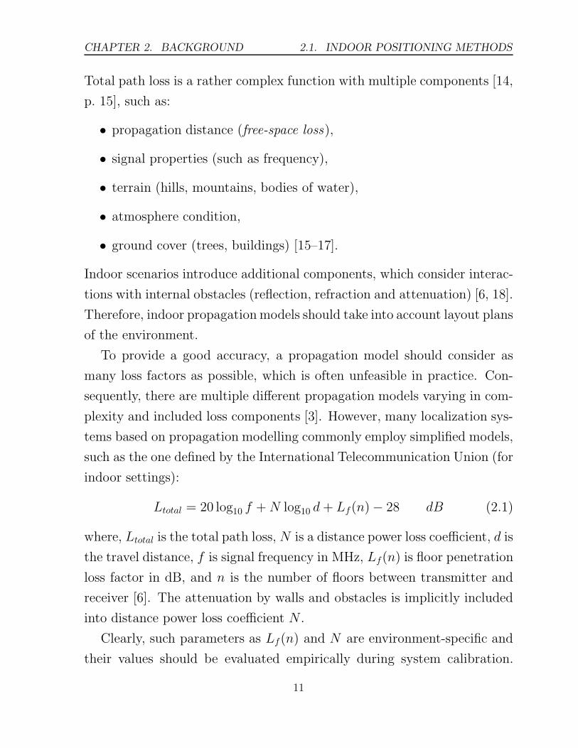
Total path loss is a rather complex function with multiple components [14,
p. 15], such as:
• propagation distance (free-space loss),
• signal properties (such as frequency),
• terrain (hills, mountains, bodies of water),
• atmosphere condition,
• ground cover (trees, buildings) [15–17].
Indoor scenarios introduce additional components, which consider interac-
tions with internal obstacles (reflection, refraction and attenuation) [6, 18].
Therefore, indoor propagationmodels should take into account layout plans
of the environment.
To provide a good accuracy, a propagation model should consider as
many loss factors as possible, which is often unfeasible in practice. Con-
sequently, there are multiple different propagation models varying in com-
plexity and included loss components [3]. However, many localization sys-
tems based on propagation modelling commonly employ simplified models,
such as the one defined by the International Telecommunication Union (for
indoor settings):
Ltotal = 20 log10 f +N log10 d+ Lf(n)− 28 dB (2.1)
where, Ltotal is the total path loss, N is a distance power loss coefficient, d is
the travel distance, f is signal frequency in MHz, Lf(n) is floor penetration
loss factor in dB, and n is the number of floors between transmitter and
receiver [6]. The attenuation by walls and obstacles is implicitly included
into distance power loss coefficient N .
Clearly, such parameters as Lf(n) and N are environment-specific and
their values should be evaluated empirically during system calibration.
11
2.1. INDOOR POSITIONING METHODS CHAPTER 2. BACKGROUND
Moreover, signal attenuation by floors (and walls) depends both on building
materials and signal frequency (9 dB at 900 MHz and 16 dB at 5.2 GHz [6,
Table 3]). If the beacons are located outdoors, the model must also con-
sider building penetration loss, which depends on building orientation, wall
materials, internal layout, floor height and windowing area [18], and varies
from 7 to 27 dB [3] or from -2 to 24 dB, increasing with frequency[18].
The major advantages of the propagation modelling are straight-forward
localization phase and good scalability. Creation of an accurate model,
however, requires a considerable effort for evaluation of site-specific char-
acteristics, such as power loss coefficients and floor layout. This approach is
best suited for line-of-sight (LOS) and obstacle-free propagation, — condi-
tions which are rarely met indoors. The positioning accuracy is determined
by the model complexity and the quality of the environment layout plan,
and is generally worse than that of fingerprinting [19, 20].
2.1.4.2 Signal fingerprinting
The signal fingerprinting is an empirical approach, which makes no assump-
tions about the environment or signal propagation paths therein [21]. This
method includes two stages: calibration and localization. The calibration
phase is a site survey comprising the collection of signal characteristics
(signal fingerprints) at predefined points, and building a database which
matches fingerprints with their locations. During the localization phase,
the mobile client acquires a fingerprint and the positioning system utilizes
the calibration data and appropriate algorithms to determine the location
to which the collected fingerprint most probably belongs.
The machine learning methods which associate fingerprints with posi-
tions during the localization phase, employ various approaches: determin-
istic and probabilistic [20, 22–24], classification and regression [25–27]. The
most popular approach is k-nearest neighbour [28], which can be attributed
12

CHAPTER 2. BACKGROUND 2.1. INDOOR POSITIONING METHODS
to its intuitiveness and good positioning results [22, 23, 25]. However, more
advanced methods can also be used: artificial neural networks [22, 23],
Bayesian inference [1, 29], support vector machines [30] or their combina-
tions [31].
The major drawback of the fingerprinting approach is the laborious
and time-consuming calibration process. Several works found that the
calibration efforts can be significantly reduced with minimal impact on
localization accuracy [19, 27, 32, 33]. Also, there are methods for automatic
acquisition of the calibration data, either with [7, 19] or without auxiliary
hardware [32, 34].
Another problem is that the localization performance of a fingerprinting
based system is prone to degradation due to changing conditions in the
environment, which result in changes in signal propagation. The dynamic
factors are air humidity, opening doors and windows, movement of people
and furniture [7, 35, 36]. To maintain the positioning accuracy in a dynamic
environment, the calibration process should be periodically repeated to
update the training dataset.
To address this, some projects employ a variety of sensors that provide
the system with updated fingerprints from predefined points in the area of
interest. Chen et al. [7] designed a Wi-Fi based positioning system that
uses RFID based sensors to provide the system with reference locations as
a user passes by. Assuming that the user walking speed is constant, the
system is able to periodically update the calibration data even between
the RFID readers. Another approaches employ a set of stationary signal
sniffers [37] or a mobile robot capable of autonomously collecting Wi-Fi
signal strength measurements in different locations [19].
This thesis, in turn, addresses the problem by introducing the novel
concept of spontaneous recalibration, which does not require any additional
hardware (see Section 3.5.1). The literature suggests that this method has
13

2.1. INDOOR POSITIONING METHODS CHAPTER 2. BACKGROUND
never been presented before.
Despite the described limitations, the fingerprinting approach provides
the best accuracy in complex environments [20, 21], such as indoors, and
works well with reflected, diffracted, and scattered signals with either LOS
or NLOS reception. Moreover, in contrast to all other methods, fingerprint-
ing does not require any knowledge about beacon positions, which makes
this method the only option for a positioning system leveraging external
beacons, such as cellular network nodes or broadcasting FM stations. The
described reasons have motivated the use of the fingerprinting approach in
this thesis.
2.1.5 Summary
Table 2.1 summarizes the localization methods discussed above.
14

CHAPTER 2. BACKGROUND 2.1. INDOOR POSITIONING METHODS
Table 2.1: Summary of indoor positioning methods.
Method Indooraccu-racy
LOS/NLOS
Affectedby mul-tipath
Cost Note
Proximity low tohigh
both no low tohigh1
• Accuracy can be improvedby additional beacons, which,however, increase the cost.
• Beacon locations must beknown.
Direction(AOA)
medium LOSonly
yes high • Accuracy depends on antenna’sangular characteristics.
• Beacon locations must beknown.
Time(TOA,TDOA)
high LOSonly
yes high • Requires precise time synchro-nization.
• Beacon locations must beknown.
Propagationmodelling
medium LOSonly
yes medium • Requires the knowledge of floorlayout and building materials.
• Beacon locations must beknown.
Finger-printing
high both no medium • Requires laborious calibration.• Beacon locations are not re-
quired.
1The cost of a proximity-based system depends on the number of beacons, which, in turn, dependson the desired accuracy.
15

2.2. STATE OF THE ART SYSTEMS CHAPTER 2. BACKGROUND
2.2 State of the art wireless indoor positioning
systems
This section presents a review of most notable state-of-the-art indoor posi-
tioning systems. The main focus is put on the radio based systems, because
unlike other signals, such as ultrasound, infrared or visible light, the ra-
dio waves can penetrate walls and thus are suitable for NLOS conditions
inherent to indoor environments.
2.2.1 Wi-Fi-based systems
Wi-Fi networks (IEEE 802.11 standard) are a popular basis for indoor posi-
tioning systems. Their popularity among the researchers can be explained
by high availability of the network infrastructure, Wi-Fi-enabled mobile
devices, and a good localization performance. Wireless networks are de-
ployed in many office buildings and homes, and the positioning system can
exploit already existing beacons.
One of the pioneering projects in RSSI-based Wi-Fi positioning was
RADAR [20]. The authors applied both propagation modelling and finger-
printing and achieved 2.94 m median error [20]; with some enhancements,
the accuracy could be increased to 2 m [38]. Ferris et al. [26] designed
a Wi-Fi localization system using Gaussian processes in conjunction with
graph-based tracking. They modeled users moving through the rooms on
the same floor, as well as more complicated patterns of moving, such as
going up and downstairs. When tested over the 3 km of test data in
a three-floor building with 54 rooms, the average error was 2.12 meters.
With advanced probabilistic methods, the median error of a Wi-Fi based
system can reach 1.2–1.45 m [39, 40].
Brunato and Battiti [30] compared the performance of Wi-Fi fingerprint-
ing localization for several machine learning methods, such as multi-layer
16

CHAPTER 2. BACKGROUND 2.2. STATE OF THE ART SYSTEMS
perceptron (MLP), support vector machine (SVM) and k-nearest neigh-
bour (kNN), both weighted and unweighted. The SVM approach demon-
strated the best median accuracy (2.75 m). Notably, the median perfor-
mance of a simple unweighted kNN classifier was only 0.16 m less, while
95th percentile errors were almost the same (6.09 m for SVM and 6.10 m
for kNN).
Chen et al. [7] investigated the dependence of the Wi-Fi positioning
accuracy on such environmental factors as humidity, doors, and people
presence. Door states (open or closed) and people presence in receiver’s
vicinity were found to have a significant impact on positioning error (236%
and 86% increase, respectively), while the humidity had smaller effect (43%
increase). While such degradation of performance is typical for fingerprint-
ing based systems, the impact of each component varies with signal fre-
quency: when the obstacles are small in comparison to wavelength, their
interaction with the wave is negligible [41, p. 132]. Therefore, environmen-
tal factors could have smaller impact on lower-frequency FM radio waves.
However, most indoor propagation measurements have been done for fre-
quencies above 1 GHz [3] and there is a lack of results for lower frequencies.
The environment dynamics also create a possibility that some beacons
present in calibration data are missing from the test set, or vice versa. This
can be caused by rearrangements of network infrastructure; a more frequent
reason, however, is the limited sensitivity of Wi-Fi modules, which cannot
detect beacon presence if its signal strength is below certain threshold. An
explicit consideration of such cases can significantly improve the positioning
accuracy [42].
Wi-Fi based positioning systems have several advantages, such as: lever-
aging the existing infrastructure, wide availability in mobile devices, and
good accuracy. However, there are also certain limitations:
Limited coverage. Despite the popularity, the coverage of Wi-Fi net-
17
2.2. STATE OF THE ART SYSTEMS CHAPTER 2. BACKGROUND
works are mostly concentrated in office buildings and dense urban
areas. Wi-Fi networks are rare in less populated cities and developing
countries [43]. Broadcasting FM stations, in contrast, transmit at high
power levels and cover areas with radius of up to several hundreds of
kilometers [44], providing almost world-wide availability. Short-range
FM transmitters, in turn, provide a cost-effective alternative to Wi-
Fi access points in areas where Wi-Fi infrastructure is not readily
available.
Interference. The 2.4 GHz industrial, scientific and medical (ISM) band
used by Wi-Fi is shared by many other electronic devices, such as
cordless phones [45] and microwave ovens [46], which may interfere
with Wi-Fi signals and affect the positioning accuracy. The FM radio
is more protected in this regard, as it operates in a dedicated frequency
band with minimal interference from other devices. Moreover, Wi-
Fi transmissions can be prohibited in sensitive environments, while
the passive FM tuners can be safely used to receive the signals from
broadcasting stations.
Power consumption. Another factor, rarely taken into account [22], is
power efficiency of the positioning system, especially on the battery-
powered mobile devices. Wi-Fi modules have a substantial power
consumption (about 300 mW in idle power-saving mode [47]), which
shortens the battery life of the mobile device. FM receivers are signifi-
cantly simpler than Wi-Fi units, and operate in passive receiving-only
mode, which results in notably longer battery life.
2.2.2 Cellular network-based systems
Cellular networks, such as GSM and CDMA, provide noticeably better
coverage than Wi-Fi. However, for a long time they were not considered
18
CHAPTER 2. BACKGROUND 2.2. STATE OF THE ART SYSTEMS
for indoor localization due to the low accuracy demonstrated in outdoor
settings [43, 48, 49].
The first results for GSM indoor positioning performance have been
published by Otsason et al. [50]. They used a GSM modem to collect wide
RSSI fingerprints which included information from 6 strongest base sta-
tions, extended by up to 35 channels which could report the RSSI but not
the Cell-ID. The experimental results for different buildings have demon-
strated a median accuracy from 3.4 to 11 m with six strongest stations,
and from 2.5 to 5.4 m with wide fingerprints. In many cases the GSM
accuracy with wide fingerprints was comparable to the Wi-Fi positioning
performance. The authors also reported that the RSSI of GSM signals was
more stable than Wi-Fi RSSI [50].
In contrast to GSM, CDMA base stations networks can dynamically
adjust their transmission power according to the network load [51], which
makes RSSI fingerprinting impractical. However, the CDMA stations are
synchronized to a common time reference (provided by GPS), which en-
ables application of time based localization methods. Using a CDMA scan-
ner, ur Rehman et al. [51] were able to evaluate signal delays from nearby
stations. Unlike the RSSI, signal delays were found to be rather stable
in time. The median localization accuracy of a system using signal delay
fingerprints reached 4.5 m (with all channels employed).
Cellular network based indoor positioning systems have three main ad-
vantages:
Coverage Unlike Wi-Fi, the GSM/CDMA networks are currently widely
available in most countries; the size of large macrocells can reach
30 km [9].
Low cost While GSM/CDMA base stations are themselves very expensive
(up to $1 million [50]), the costs are covered by the cellular network op-
19

2.2. STATE OF THE ART SYSTEMS CHAPTER 2. BACKGROUND
erator (and ultimately, the subscribers). Thus, the positioning system
can exploit readily available stations and does not require installation
of a dedicated indoor infrastructure as Wi-Fi does.
Battery life Although a cellular transceiver module is rather battery-
consuming even in an idle state [52], in many scenarios it remains
powered in order to provide the voice or data connectivity. Thus, the
overhead introduced by a positioning system relates only to location
estimation and excludes powering additional wireless module, which
is often the case for Wi-Fi.
However, GSM/CDMA positioning has also several shortcomings:
Low accuracy The presented works rely on the use of wide fingerprints
in order to provide a good accuracy. Acquisition of extended data,
however, required special hardware (programmable GSM modem and
CDMA scanner). With the narrow fingerprints which could be ac-
quired with conventional hardware, the localization accuracy was rather
low.
Low reliability Given that GSM/CDMA beacons are situated outdoors,
the signal propagation conditions vary due to environmental factors,
such as weather and terrain. In particular, radio signals with frequen-
cies above 1 GHz are affected by rain scatter interference [53, p. 8] and
terrain vegetation [17]; trees in leaf can cause a 20% higher attenuation
than leafless trees [17, p. 3]. In theory, these factors can significantly
affect the positioning performance; however, no experimental studies
are available yet.
20

CHAPTER 2. BACKGROUND 2.2. STATE OF THE ART SYSTEMS
2.2.3 FM radio-based systems
There are only few works dedicated to FM radio based positioning. The
first localization system based on FM radio signals was presented by Krumm
et al. [54]. It was an outdoors-only positioning system that employed a pro-
totype wristwatch device (with an FM receiver) to distinguish six districts
of Seattle using the signals broadcast from public FM stations. The au-
thors were able to identify the correct district in about 80% of cases. More
advanced algorithms, combined with propagation modelling, enabled the
system to locate the user with 8 km median accuracy [1].
Fang et al. [2] presented a comparison of FM and GSM outdoor localiza-
tion within 20 reference points in an urban area of about 1 km2. Using the
data collected with a professional spectrum analyzer, the authors demon-
strated that with six-channel fingerprints the GSM accuracy was better
than that of FM; however, when the number of FM channels was increased
to 11 the situation reversed (error below 20 m in 67% of cases). In a rural
area, however, GSM signals were weaker and 5-channel FM positioning
outperformed the 8-channel GSM based system; the FM positioning error
was within 35 m with 67% probability. Unfortunately, the reported data
is not suffucient to compare FM accuracy in urban and rural areas for
equal number of used channels. The authors also reported better temporal
stability of FM signals in comparison to GSM.
Recently, the same group evaluated the positioning performance of mul-
tiple wireless technologies (FM, GSM, DVB, Wi-Fi) in both outdoor and
indoor settings. However, FM measurements were performed only out-
doors [55] and therefore FM positioning was not included into comparison
of indoor localization systems.
All the systems described above utilize the differences of signal strength
between different locations. The two main sources of signal attenuation
(leading to spatial variation of the fingerprints) in outdoor settings are:
21

2.2. STATE OF THE ART SYSTEMS CHAPTER 2. BACKGROUND
free-space propagation loss (in order of 20 log d, where d is travel distance)
and shadowing by terrain and buildings [14, 56]. In [2], the distance be-
tween test points was about 100 m, and free-space propagation loss con-
tributed about 40 dB to the signal strength differences between locations.
At indoor scales, however, the free-space propagation loss is negligible and
the main source of spatial signal variation is fast fading caused by indoor
obstacles and multipath propagation [6, 14]. Thus, the discussed FM po-
sitioning systems rely on outdoor-only propagation phenomena and their
results cannot be simply scaled down to indoor scenario.
In 1994, Giordano et al. [57] proposed (and patented [58–60]) an FM
based outdoor localization system which leverages differences of FM stereo
pilot phase (see Section 2.3.3), as received by the mobile unit and a fixed
observer. The authors claimed the accuracy “on the order of 10–20 m de-
pending on channel conditions” [57, p. 1144]. However, the origins of these
numbers are questionable, since the authors have not provided any exper-
imental proofs of the claimed performance. Moreover, there are certain
indications that the pilot tone, although transmitted with a good stability,
is distorted by multipath [61, 62] and non-linear effects in the receiver [63,
p. 5]. For instance, typical peak-to-peak pilot phase fluctuations observed
by Howe [62] were of about 2 µs, which corresponds to about 600 m dis-
tance for a 19 kHz pilot tone. Such a low accuracy is unsuitable for indoor
positioning, and the phase-difference approach is listed in this thesis only
for completeness.
Broadcasting FM stations can also be employed as “illuminators of op-
portunity” for passive coherent location (PCL) systems [64, 65]. PCL sys-
tems exploit civilian ground-based stations such as FM radio, digital and
analog TV, cellular networks as the transmitters in bistatic radar setup
(spatially separated stationary transmitter and receiver). This setup is ef-
fective against stealth technology, while passive receivers make the radars
22
CHAPTER 2. BACKGROUND 2.2. STATE OF THE ART SYSTEMS
less vulnerable for electronic counter measures. By correlating the direct
and target-scattered signals, a PCL system is able to estimate the distance
to the target. FM-based PCL systems have a theoretical range resolution
of up to 1 km [66] with the coverage of tens of kilometers [64]. PCL sys-
tems, however, are largely out of the scope of this thesis and are mentioned
only for completeness.
As the literature shows, the previous works have focused only on outdoor
localization using broadcast FM signals and special receivers (prototype
wristwatch [1], professional spectrum analyzer [2] and special radar equip-
ment [64, 66]). This thesis, in contrast, focuses on indoor positioning with
consumer-grade mobile devices. This is first study of indoor localization
using FM-band radio signals.
2.2.4 Other systems
While Wi-Fi and cellular networks represent the prevailing infrastructures
for indoor localization due to their availability, there are many other posi-
tioning technologies. This section presents a short overview of the relevant
systems and an analysis of their properties.
Practically every Wi-Fi enabled mobile device, such as cellphone or
computer, also has an embedded Bluetooth module. The distance range
of the typical class-II devices is 10 m. Moreover, Bluetooth hardware and
communication protocol have been designed with a focus on low power
consumption. All of this makes Bluetooth an interesting technology for
indoor positioning, and there are several works dedicated to Bluetooth
based localization systems [67, 68]. However, the coverage of such systems
is very limited due to the short range of Bluetooth modules, and, more
importantly, the lack of stationary Bluetooth devices. Another drawback
is that each location acquisition runs the device discovery procedure; this
significantly increases both the localization latency (10–30 s) and power
23

2.2. STATE OF THE ART SYSTEMS CHAPTER 2. BACKGROUND
consumption. Therefore, Bluetooth is commonly agreed [67] to be unsuit-
able for localization systems.
Ultra-wide band (UWB) systems, on contrary, demonstrate very good
localization accuracy. The commercially available indoor localization sys-
tem Ubisense [69] employs TDOA and AOA methods for UWB radio sig-
nals and is capable of achieving 15 cm accuracy in three dimensions. How-
ever, the system has a very high cost which severely impacts wide adoption.
Radio Frequency IDentification (RFID) technology is widely used for
asset tracking and shop security systems. Due to the short communication
range (dozens of centimeters), it provides a good localization accuracy. The
short reading distance, however, also significantly limits its possible appli-
cation areas. While RFID based systems can accurately detect proximity
and are used for activity recognition [70], a wide-scale indoor localization
requires a dense infrastructure of either tags (for mobile reader) or readers
(for mobile tags). The limited coverage and sporadic location updates make
RFID based systems unsuitable for general-purpose indoor localization.
An interesting approach to indoor positioning has been proposed by [71].
The system included two beacons which injected radio frequency (RF) sig-
nals into domestic powerline. These signals were then detected by a spe-
cialised receiver and associated with the user’s location using the finger-
printing approach. An extended, wide-band version of the system achieved
a room-level accuracy of 90% [72]. While only two beacons are sufficient for
an entire building, the system relies on specialised hardware with limited
availability.
Digital Enhanced Cordless Telecommunication (DECT) phones, despite
their popularity in Europe, have received little attention with regard to
their suitability for indoor localization. This can be explained by limited
availability of DECT systems capable of providing signal information to
external devices (such as computers or smartphones) and high cost of such
24

CHAPTER 2. BACKGROUND 2.2. STATE OF THE ART SYSTEMS
systems. However, recently, Kranz et al. [73] presented a DECT position-
ing system employing an open DECT stack implementation. The authors
demonstrated that in all indoor scenarios DECT localization outperformed
the Wi-Fi based system. This can be explained by the relatively high trans-
mission power of DECT stations (up to 250 mW [74, p. 27]), which results
in significantly higher number of DECT stations in each fingerprint, in
comparison to Wi-Fi.
Contrary to indoor results, the accuracy of DECT localization in out-
door scenario was lower than Wi-Fi, despite the larger number of DECT
stations. This demonstrates that the differences between indoor and out-
door environments with regard to localization accuracy vary depending on
the environment, and a low accuracy outdoors is not necessarily the case
indoors. Thus, the low outdoors accuracy of FM radio based systems dis-
cussed in previous section, cannot constitute a basis for assumptions about
FM radio’s applicability for indoor localization.
While DECT presents an interesting opportunity for localization sys-
tems, its coverage is currently limited to European urban environments; no
DECT signals were detected in US [75]. DECT based localization would
also require hardware modifications of the mobile devices. These reasons
significantly limit the feasibility of DECT localization at the present time.
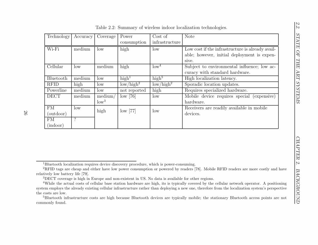
2.2.5 Summary
A summary of the wireless positioning technologies discussed above is pre-
sented in Table 2.2.
25
2.2.
STATE
OFTHEART
SYSTEMS
CHAPTER
2.
BACKGROUND
Table 2.2: Summary of wireless indoor localization technologies.
Technology Accuracy Coverage Powerconsumption
Cost ofinfrastructure
Note
Wi-Fi medium low high low Low cost if the infrastructure is already avail-able; however, initial deployment is expen-sive.
Cellular low medium high low4 Subject to environmental influence; low ac-curacy with standard hardware.
Bluetooth medium low high1 high5 High localization latency.RFID high low low/high2 low/high2 Sporadic location updates.Powerline medium low not reported high Requires specialized hardware.DECT medium medium/
low3
low [76] low Mobile device requires special (expensive)hardware.
FM(outdoor)
lowhigh low [77] low
Receivers are readily available in mobiledevices.
FM(indoor)
?
1Bluetooth localization requires device discovery procedure, which is power-consuming.2RFID tags are cheap and either have low power consumption or powered by readers [78]. Mobile RFID readers are more costly and have
relatively low battery life [79].3DECT coverage is high in Europe and non-existent in US. No data is available for other regions.4While the actual costs of cellular base station hardware are high, its is typically covered by the cellular network operator. A positioning
system employs the already existing cellular infrastructure rather than deploying a new one, therefore from the localization system’s perspectivethe costs are low.
5Bluetooth infrastructure costs are high because Bluetooth devices are typically mobile; the stationary Bluetooth access points are notcommonly found.
26
CHAPTER 2. BACKGROUND 2.3. FM RADIO TECHNOLOGY
2.3 FM radio technology
This section provides background information about FM radio technology
and its specifics. This material is necessary for complete understanding of
some aspects of the proposed approach.
2.3.1 Overview
Despite its considerable age, FM radio is still very popular. It is widely
available across the world, and most households have even more than one
receiver [80, p. 7]. Car manufacturers consider FM radio as a de-facto
standard feature [80]. Although currently there are global trends of sub-
stituting analog broadcasts by digital ones, the European Radio Spectrum
Policy Group notes that “there is no indication of any progress anywhere
to cease analogue radio in the foreseeable future” [80].
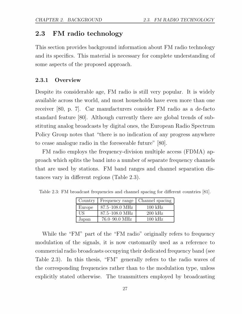
FM radio employs the frequency-division multiple access (FDMA) ap-
proach which splits the band into a number of separate frequency channels
that are used by stations. FM band ranges and channel separation dis-
tances vary in different regions (Table 2.3).
Table 2.3: FM broadcast frequencies and channel spacing for different countries [81].
Country Frequency range Channel spacing
Europe 87.5–108.0 MHz 100 kHzUS 87.5–108.0 MHz 200 kHzJapan 76.0–90.0 MHz 100 kHz
While the “FM” part of the “FM radio” originally refers to frequency
modulation of the signals, it is now customarily used as a reference to
commercial radio broadcasts occupying their dedicated frequency band (see
Table 2.3). In this thesis, “FM” generally refers to the radio waves of
the corresponding frequencies rather than to the modulation type, unless
explicitly stated otherwise. The transmitters employed by broadcasting
27
2.3. FM RADIO TECHNOLOGY CHAPTER 2. BACKGROUND
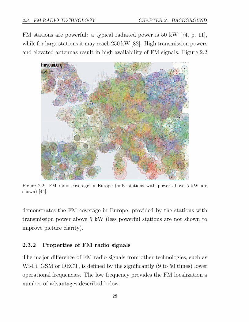
FM stations are powerful: a typical radiated power is 50 kW [74, p. 11],
while for large stations it may reach 250 kW [82]. High transmission powers
and elevated antennas result in high availability of FM signals. Figure 2.2
Figure 2.2: FM radio coverage in Europe (only stations with power above 5 kW areshown) [44].
demonstrates the FM coverage in Europe, provided by the stations with
transmission power above 5 kW (less powerful stations are not shown to
improve picture clarity).
2.3.2 Properties of FM radio signals
The major difference of FM radio signals from other technologies, such as
Wi-Fi, GSM or DECT, is defined by the significantly (9 to 50 times) lower
operational frequencies. The low frequency provides the FM localization a
number of advantages described below.
28

CHAPTER 2. BACKGROUND 2.3. FM RADIO TECHNOLOGY
Firstly, FM signals are less affected by weather conditions. The rec-
ommendations of the International Telecommunication Union suggest that
rain scatter interference is negligible for frequencies below 1 GHz [53, 83,
p. 8], while fog and clouds can be ignored for up to 10 GHz [16].
Secondly, low frequency radio waves are less sensitive to the terrain
conditions. In particular, the specific attenuation in woodland at 100 MHz
is typically about 0.04 dB/m, while for GSM frequencies (0.9/1.8 GHz)
the attenuation increases to 0.1–0.3 dB/m, with additional 20% for trees
in leaf [17]. The foliage movement due to wind may produce additional
attenuation at higher frequencies [17]. FM signals are thus not affected by
these minor influences.
Thirdly, the attenuation of radio waves by building materials increases
with frequency [41, 74] and thus FM signals penetrate walls more easily
than Wi-Fi or GSM. This ensures high availability of positioning signals
in indoor settings.
Finally, the FM wavelength of about 3 m results in different interac-
tion with most indoor objects, as compared to 0.12 m Wi-Fi waves. At
low frequencies, when the obstacles are small compared to wavelength,
they do not interact significantly with the electromagnetic fields of the
wave [41, p. 132]. However, when the size of an obstacle is comparable to
the wavelength, interaction is very strong and produces complex interfer-
ence patterns [14, 41]. Ultimately, this means that most indoor objects are
transparent for long FM radio waves, but do interact with shorter Wi-Fi
and GSM signals. Clearly, this makes FM signals less perceptive to small
object movements than Wi-Fi or GSM.
The described considerations suggest that FM based indoor positioning
has a number of theoretical advantages over the current high-frequency
systems.
29
2.3. FM RADIO TECHNOLOGY CHAPTER 2. BACKGROUND
2.3.2.1 Capture effect
For amplitude modulated signals, when two stations broadcast on the same
or nearby frequencies, both of them will be heard at the receiver side. This,
however, is not the case for frequency modulation, which is inherently
more robust to interference. Due to the so-called FM capture effect, only
the station with the strongest signal will be demodulated and reach the
receiver’s output, while the other will be attenuated to a high degree [84]
(assuming that both signal levels are above the capture threshold [85]).
The capture effect enables situations when several FM beacons can oc-
cupy the same frequency channels without interfering with each other. The
receiver will notice only the strongest beacon.
2.3.3 Stereo FM and RDS
Due to relatively wide channels, FM broadcasts may include more infor-
mation than just monophonic audio, and transmit also stereo sound and
digital data.
The currently used stereophonic multiplexing scheme has been proposed
by Zenith Corp. and General Electric Company [86]. Although its stereo-
phonic quality was somewhat lower than that of a competing system, it
had smaller losses for monophonic reception and had significantly lower
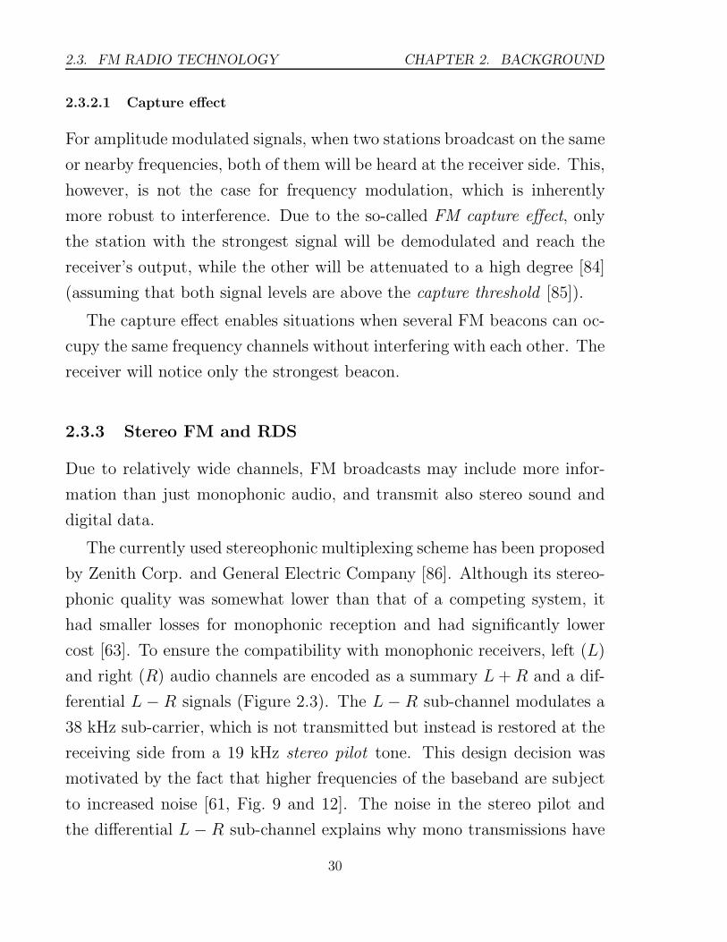
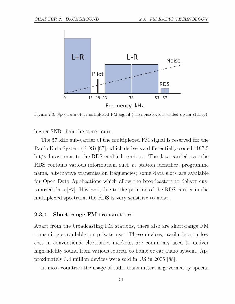
cost [63]. To ensure the compatibility with monophonic receivers, left (L)
and right (R) audio channels are encoded as a summary L+ R and a dif-
ferential L − R signals (Figure 2.3). The L − R sub-channel modulates a
38 kHz sub-carrier, which is not transmitted but instead is restored at the
receiving side from a 19 kHz stereo pilot tone. This design decision was
motivated by the fact that higher frequencies of the baseband are subject
to increased noise [61, Fig. 9 and 12]. The noise in the stereo pilot and
the differential L − R sub-channel explains why mono transmissions have
30
CHAPTER 2. BACKGROUND 2.3. FM RADIO TECHNOLOGY
Figure 2.3: Spectrum of a multiplexed FM signal (the noise level is scaled up for clarity).
higher SNR than the stereo ones.
The 57 kHz sub-carrier of the multiplexed FM signal is reserved for the
Radio Data System (RDS) [87], which delivers a differentially-coded 1187.5
bit/s datastream to the RDS-enabled receivers. The data carried over the
RDS contains various information, such as station identifier, programme
name, alternative transmission frequencies; some data slots are available
for Open Data Applications which allow the broadcasters to deliver cus-
tomized data [87]. However, due to the position of the RDS carrier in the
multiplexed spectrum, the RDS is very sensitive to noise.
2.3.4 Short-range FM transmitters
Apart from the broadcasting FM stations, there also are short-range FM
transmitters available for private use. These devices, available at a low
cost in conventional electronics markets, are commonly used to deliver
high-fidelity sound from various sources to home or car audio system. Ap-
proximately 3.4 million devices were sold in US in 2005 [88].
In most countries the usage of radio transmitters is governed by special
31
2.4. SUMMARY CHAPTER 2. BACKGROUND
regulations. While Wi-Fi is widely adopted and generally does not re-
quire licensing, different rules may apply to short-range FM transmitters,
depending on local laws.
In EU countries, the usage of short-range FM transmitters operating
within 88–108 MHz frequency band is governed by European Commission
Decision 2009/381/EC [89]. According to it, the FM transmitters with
effective radiated power of less than 50 nW do not require licensing. Com-
plying devices bear the “CE” certification mark. In US, all radio devices
must comply with the FCC Part 15 regulations. In particular, a short-
range FM transmitter must produce less that 250 mV field strength in an
average receiver placed 3 m away [90, Section 15.239b]. The device can be
used only with the antenna furnished with it [90, Section 15.203] (Euro-
pean regulations do not include this requirement). Certified devices have
an explicit statement of their conformity to the FCC Part 15 regulations.
For home-build transmitters, there is an additional limit of no more than
five devices per person [90, Section 15.23a].
2.4 Summary
The analysis of the state of the art demonstrates that at the moment there
are no perfect indoor localization systems reported in the literature. The
major problems are limited coverage (Wi-Fi, Bluetooth, RFID, powerline,
DECT), high power consumption (Wi-Fi, cellular, mobile RFID readers),
low accuracy (GSM) and high hardware costs (Bluetooth access points,
powerline, RFID readers, specialized DECT receivers).
FM radio stations, in contrast, provide worldwide coverage; FM re-
ceivers are already embedded in many mobile devices and have small power
consumption. However, in the current literature the accuracy of FM based
positioning has been evaluated in outdoor settings only and there are no
32

CHAPTER 2. BACKGROUND 2.4. SUMMARY
results for its indoor performance. This gap is addressed by the present
thesis.
33


Chapter 3
Indoor positioning using FM radio
signals
This chapter introduces the FM radio based positioning system, analyze
the features it relies upon and provide an in-depth description of the used
methods and techniques.
3.1 Proposed approach
The indoor positioning system proposed in this thesis is based on finger-
printing of FM radio signals. As stated in Section 2.1.4.2, the fingerprinting
approach is well-suited for indoor conditions, characterized by multipath
and non-line-of-sight (NLOS) propagation, refraction and attenuation by
internal obstacles, such as walls, furniture and smaller objects [3]. De-
spite the complex conditions, fingerprinting provides a good accuracy with
minimal infrastructure costs [21, 91]. Clearly, while the proximity-based
systems are easy to implement, their accuracy directly depends on the
spatial density of the beacons. Better accuracy requires more beacons and
increases both hardware and deployment costs. The systems based on the
direction of signal arrival require sophisticated antenna arrays which are ex-
pensive and can be too large for some environments. Time-based systems,
35

3.1. PROPOSED APPROACH CHAPTER 3. FM POSITIONING
as mentioned in Section 2.1.3, can provide high positioning accuracy, but
require precise synchronisation of beacon clocks and suffer from multipath
and NLOS propagation typical for indoors. The systems based on finger-
printing are well-suited for complex environments and demonstrate good
performance with relatively small number of beacons (Section 2.1.4.2).
In this work, two types of FM radio transmitters (beacons) are consid-
ered:
• local beacons, such as short-range transmitters deployed in the indoor
environment (referenced as FML hereinafter);
• external beacons, such as broadcasting FM stations (referenced as
FMB).
Local beacons can be installed at arbitrary locations, where the positioning
system is to be used. Additional beacons improve the accuracy of the
system (which depends on the spatial density of the beacons), but increase
the infrastructure costs. An FM positioning system with local beacons
has substantionally lower cost than an equivalent Wi-Fi based system, yet
demonstrates comparable or better performance (see Chapter 4).
In the case of broadcasting stations, it is impossible to set the posi-
tion of the beacons, their number or the transmitted signals. Thus, it is
difficult to predict the accuracy of the system in different areas without
actual measurements. However, this kind of system does not require any
additional infrastructure, which can be a significant advantage over other
indoor positioning systems. An experimental evaluation of this approach
(Chapter 5) demonstrates that accuracy of an FMB positioning system is
comparable with that of other systems.
This thesis focuses mainly on self-positioning paradigm [91], whereby
the mobile device estimates its location using the signals received from the
beacons. An inverse approach, where a number of interconnected station-
36
CHAPTER 3. FM POSITIONING 3.1. PROPOSED APPROACH
ary receivers estimate the location of a mobile transmitter, could also be
possible. However, this approach has a number of disadvantages in compar-
ison to self-positioning using FM radio signals. A radio transmission from
the mobile device would significantly impact its battery life. Moreover, it
could also possibly affect user’s privacy, as in a network-based positioning
system the user has no control over processing of the location information.
In the FM-based self-positioning approach, in contrast, the mobile unit is
merely a receiver, invisible to the beacons, and sensitive location data can
be processed locally by the mobile device, thus ensuring user’s privacy. Due
to the described reasons, the proposed FM localization system employs the
self-positioning approach.
In any positioning system, there are two core components:
• a method for distinguishing different reference points (beacons), and
• a measure of distance or angle between the mobile unit and the bea-
cons.
Beacon identity is usually encoded in the signal it transmits. While in
many systems this information is easily available from the hardware layer
(MAC address for Wi-Fi and Bluetooth, Cell-ID for GSM, tag number
for RFID), FM radio has not been initially designed to deliver machine-
understandable station ID. This thesis proposes several ways to identify
a beacon within an FM positioning system, such as: by radio channel,
using audio-encoded message, and using RDS data. An analysis of these
methods, their features and limitations, will be presented in Section 3.3.
The literature review in Section 2.1 suggests a variety of distance-
dependent features of radio signals. The most prominent and widely used
feature is the strength of the received radio signal (RSS), or its representa-
tion by the receiver’s hardware, called the received signal strength indicator
(RSSI ). An FM radio signal, however, also carries a lower-frequency audio
37
3.2. DISTANCE-DEPENDENT FEATURES CHAPTER 3. FM POSITIONING
component which could provide distance information. This thesis identified
four distance-dependent features suitable for FM-based localization:
• received signal strength indicator (RSSI),
• audio signal-to-noise ratio (SNR),
• stereo channel separation (SCS), and
• phase of the stereo pilot tone.
Although the last feature has been found to be unsuitable for indoor po-
sitioning, it is included for completeness. The audio-based methods (SNR
and SCS) demonstrated limited dependence on the transmitter-to-receiver
distance. The main focus of this thesis is dedicated to the RSSI, which
yielded the best positioning performance. A detailed analysis of distance-
dependent features is presented in the following section.
3.2 Distance-dependent features of FM radio signal
The relative position of the user with regard to a beacon can be char-
acterised by the angle between directed antennas, signal propagation time
and certain properties of the received signal. For the FM radio, a set of four
distance-dependent feature candidates have been identified within this the-
sis, namely: received signal strength, audio signal quality (represented by
signal-to-noise ratio), separation of stereo channels, and pilot tone phase.
The following sections discuss each feature in detail.
3.2.1 Received signal strength
Received signal strength indicator (RSSI) is one of the most popular feature
used for positioning (see Section 2.1.4.2). The RSSI corresponds to the
amplitude of the received radio-frequency signal. It can be expressed in
38

CHAPTER 3. FM POSITIONING 3.2. DISTANCE-DEPENDENT FEATURES
decibels or in abstract units, such as percents or even categorical values
like “excellent” or “poor”. Most of the current FM receivers employ the
RSSI to provide seek tuning functionality [77]; some of them also provide
the RSSI value to the software layer.
Theoretically, received signal strength is inversely proportional to the
square of travel distance (see Section 2.1.4.1). In practice, however, the
RSSI dependence on distance is subject to multiple factors, such as envi-
ronment properties, transmitter and receiver characteristics (power, sensi-
tivity, signal processing methods).
In order to evaluate the applicability of the RSSI for FM positioning, two
tests with local short-range FM transmitters [92] were performed. The re-
ceiver employed in both tests was Nokia N800, which distinguishes 16 RSSI
levels (see Appendix B.1).
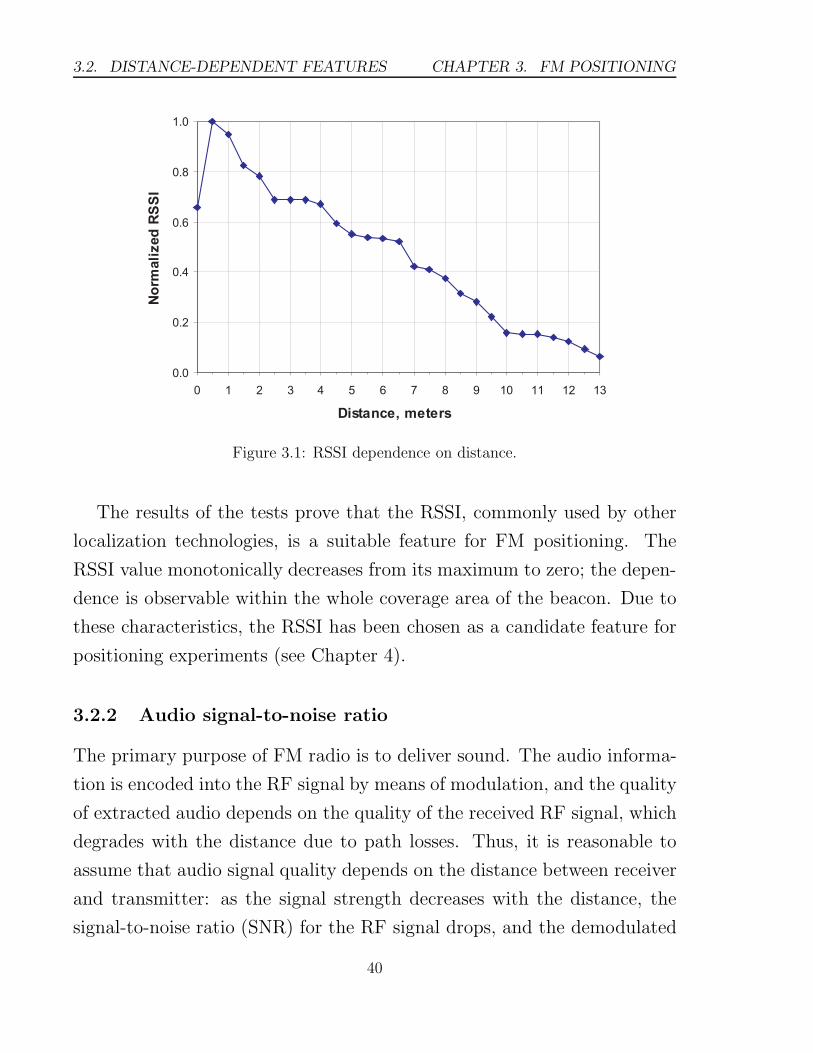
The first test evaluated the RSSI dependence on the distance from the
transmitter. To avoid any interference from furniture, this test was per-
formed outdoors. The results are presented in Figure 3.1. The RSSI de-
pendence on distance is relatively smooth and monotone starting from
0.5 m, and proves the RSSI to be a suitable feature for positioning1. The
plateau-looking areas can be explained by the limited number of RSSI
levels recognized by the receiver used in the test.
In the second test, the measurements were performed indoors. Fig-
ure 3.2a shows the RSSI from three transmitters (represented by antenna
signs in Figure 3.2b) while the user was moving from Transmitter 1 to
Transmitter 3 along the dashed line in the floorplan. Although the depen-
dencies are not very smooth, which is caused by the distortions from the
furniture and multipath propagation, the general trends, nevertheless, are
clearly observable.
1The RSSI values at distance “0” have been measured in the close vicinity of the transmitter’s antenna,which constitutes the near-field region of the radiation, where reactive component dominates the distanceone [74, p. 46]. Therefore the RSSI near the antenna does not follow the general trend.
39
3.2. DISTANCE-DEPENDENT FEATURES CHAPTER 3. FM POSITIONING
Figure 3.1: RSSI dependence on distance.
The results of the tests prove that the RSSI, commonly used by other
localization technologies, is a suitable feature for FM positioning. The
RSSI value monotonically decreases from its maximum to zero; the depen-
dence is observable within the whole coverage area of the beacon. Due to
these characteristics, the RSSI has been chosen as a candidate feature for
positioning experiments (see Chapter 4).
3.2.2 Audio signal-to-noise ratio
The primary purpose of FM radio is to deliver sound. The audio informa-
tion is encoded into the RF signal by means of modulation, and the quality
of extracted audio depends on the quality of the received RF signal, which
degrades with the distance due to path losses. Thus, it is reasonable to
assume that audio signal quality depends on the distance between receiver
and transmitter: as the signal strength decreases with the distance, the
signal-to-noise ratio (SNR) for the RF signal drops, and the demodulated
40
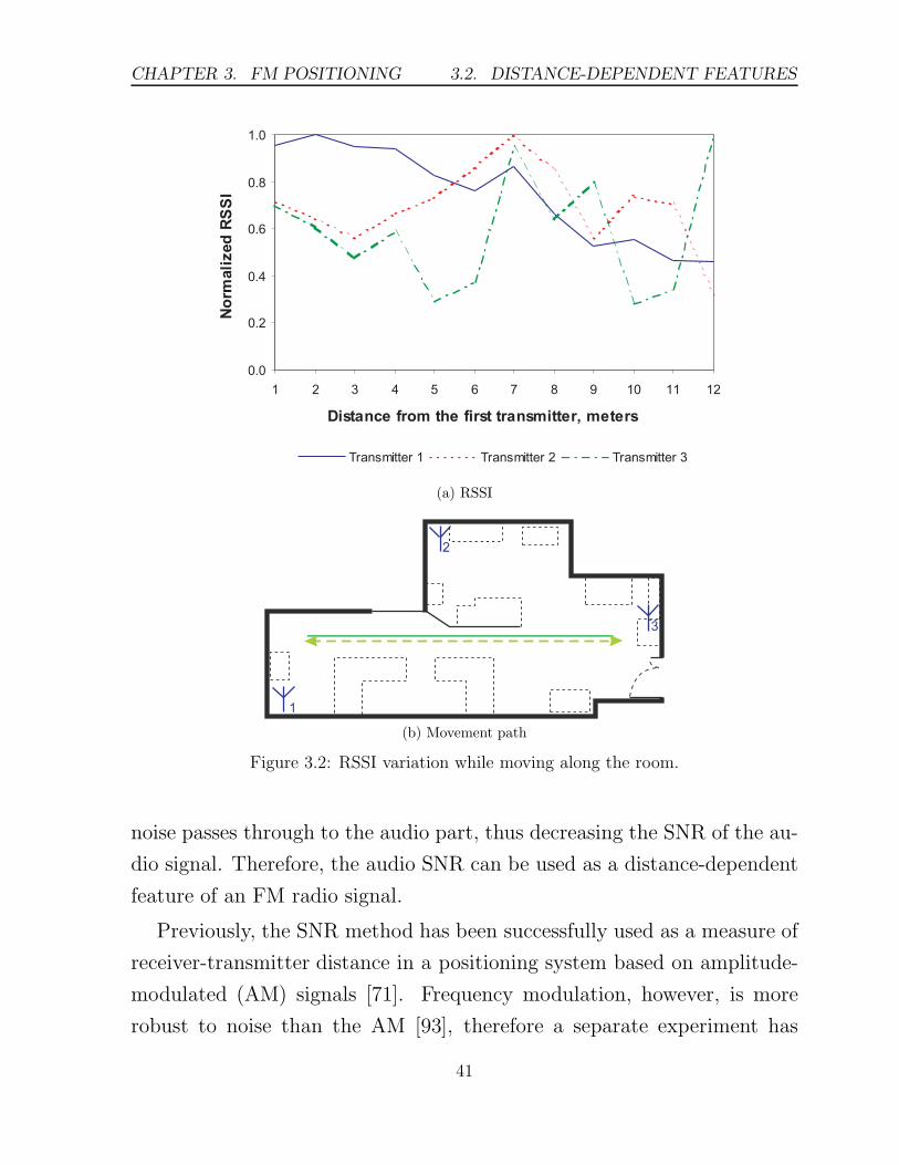
CHAPTER 3. FM POSITIONING 3.2. DISTANCE-DEPENDENT FEATURES
(a) RSSI
(b) Movement path
Figure 3.2: RSSI variation while moving along the room.
noise passes through to the audio part, thus decreasing the SNR of the au-
dio signal. Therefore, the audio SNR can be used as a distance-dependent
feature of an FM radio signal.
Previously, the SNR method has been successfully used as a measure of
receiver-transmitter distance in a positioning system based on amplitude-
modulated (AM) signals [71]. Frequency modulation, however, is more
robust to noise than the AM [93], therefore a separate experiment has
41

3.2. DISTANCE-DEPENDENT FEATURES CHAPTER 3. FM POSITIONING
been performed to evaluate the relationship between distance and audio
SNR of FM radio.
To test the applicability of audio SNR method for FM positioning, a
short-range FM transmitter has been set to broadcast a continuous dual
tone multi-frequency (DTMF) signal for digit “1”, compose of 1209 Hz and
697 Hz sine waves. At the client side, the signal was received by a conven-
tional FM radio (Creative MuVo TX FM). The audio signal was sampled
by a laptop sound card at 8 kHz sampling frequency and transformed to
the frequency domain using 1024-band FFT. For each distance, 32 spectra
were recorded and then averaged. The SNR was then calculated as follows:
SNR =band697Hz + band1209Hz
mean(all bands)
The experiment discovered no clear dependency of audio SNR from the
distance to the transmitter (see Figure 3.3). The distances from 0 to about
Figure 3.3: Audio SNR dependence on distance.
0.6 m correspond to near field of the antenna[74, p. 46] and are not relevant
for positioning. In range from 0.9 m to 3.6 m the mean SNR value remained
42

CHAPTER 3. FM POSITIONING 3.2. DISTANCE-DEPENDENT FEATURES
almost constant (varied within 5%), between 3.6 m and 4.5 m it became
unstable, and then rapidly degraded to the noise level. Such behaviour can
be explained by the FM capture effect which improves the post-detection
SNR for non-linear modulations (such as FM) when the pre-detection SNR
is above a certain level, called “capture threshold”; below this threshold the
SNR drops dramatically [85].
However, the observed behavior can also be attributed to the receiver’s
noise-reduction circuitry which automatically mutes the audio output if
the received signal is too weak [94]. To verify this hypothesis, a separate
experiment has been performed with a programmable FM tuner with auto-
mute feature disabled.
Figure 3.4: Audio SNR dependence on distance (auto-mute off).
The results in Figure 3.4 confirm the assumption, and demonstrate that
audio SNR does in fact reflect the distance from the signal source, even
though the dependence is less smooth than in the case of RSSI (see Fig-
ure 3.1). At short distances, the reception quality is almost perfect, and
SNR is limited by the SNR characteristics of the transmitter and receiver.
43

3.2. DISTANCE-DEPENDENT FEATURES CHAPTER 3. FM POSITIONING
As the distance increases, the SNR declines.
Thus, audio SNR can be utilized as a distance-dependent feature, pro-
vided that audio quality augmentation features of the receiver are switched
off. The positioning performance of the SNR approach is evaluated in Sec-
tion 4.1.3.
3.2.3 Stereo channel separation
The FCC rules [95] define “stereophonic separation” as
The ratio of the electrical signal caused in sound channel A to
the signal caused in sound channel B by the transmission of only
a channel B signal. Channels A and B may be any two channels
of a stereophonic sound broadcast transmission system.
The motivation for considering the stereo channel separation (SCS) as
a measure of distance is two-fold. Firstly, the stereophonic signal is more
sensitive to noise than the monophonic one [63]. At the same RSS level,
the SNR difference between the two modes can reach 20 dB [61, Fig. 12].
The inherent white noise of the RF signal transforms after the detection
to a noise linearly increasing with the frequency [61, Fig. 9]. As described
in Section 2.3.3, this noise mostly affects the pilot subcarrier and the dif-
ferential L − R part of the stereo signal, where L and R denote the left
and the right audio channels, respectively. The summary L + R signal,
however, is less affected. Secondly, the quality of the stereo signal strongly
depends on the quality of the received pilot subcarrier and distortions in
the pilot affect the quality of the stereo signal. When the distance to the
beacon increases and the RF signal quality degrades, the differential L−R
part of the audio signal is affected the most, and the receiver gradually
combines the stereo channels to maintain the sound quality [77, p. 17].
44

CHAPTER 3. FM POSITIONING 3.2. DISTANCE-DEPENDENT FEATURES
Consequently, the L + R part will dominate in the output of the receiver,
which results in the reduction of stereo channel separation.
Figure 3.5: Stereo channel separation (SCS) dependence on distance.
Figure 3.5 shows the experimental results for SCS dependence on dis-
tance to the beacon (the experimental setup is described in Appendix B.2).
As the distance increases, the SCS quickly deteriorates, reaches its mini-
mum and remains constant while the distance grows further. The minimum
of the SCS corresponds to no channel separation, or monophonic mode.
The use of stereo channel separation as a measure of distance is unique
for FM positioning and, according to the literature, has never been evalu-
ated before. However, it has certain limitations. First of all, the beacons
must transmit a known stereo signal, so that the client can estimate the
cross-talk between the channels. This limits the SCS approach to local bea-
cons only, as the signal of broadcasting FM stations (voice, music) changes
dynamically and is generally unknown. Secondly, the SCS method is usable
in a smaller range of distances than the RSSI one, as when the distance
— and hence the noise — increases, it becomes impossible to maintain
the stereo decoding, and the receiver switches to monophonic mode, ef-
45

3.2. DISTANCE-DEPENDENT FEATURES CHAPTER 3. FM POSITIONING
fectively converging the channel separation to zero. The RSSI, however,
remains non-zero and sufficient to keep mono reception. The experimental
evaluation of the FM positioning system based on the SCS approach is
presented in Section 4.1.3
3.2.4 Stereo pilot phase
All stereophonic FM transmissions contain a special signal, known as pi-
lot tone, which is required to decode the multiplexed audio signal (Sec-
tion 2.3.3). The stability of this 19 KHz pilot defines the quality of the
output stereo signal and therefore the accuracy of the pilot tone is guar-
anteed by the corresponding standards [96].
Provided that the pilot signal is very stable, it might be possible to use
the phase difference of pilot tones from multiple stations to estimate the
client position. This idea is presented in [57] and a number of patents [60,
97]. For example, US patent #5689270 [60] proposes to estimate distance
between the client and a reference point using the the phase difference of
the pilot measured at these two locations. To acquire the position of the
client, multiple FM signals (pilot tones) must be collected.
However, this approach is unsuitable for indoor positioning. Despite
the pilot stability at the transmitting side, in real world its phase at the
receiver is subject to distortions caused by RF channel conditions, receiver
noise [63, p. 5], and multipath propagation [61, 62, Fig. 17], which is typical
for indoor environments. The experiments conducted by Howe [62] show
that a typical jitter of the pilot tone phase is about 2 µs; given the pilot
frequency of 19 kHz and thus the wavelength of about 15 km, the jitter
would result in about 600 m positioning error. Clearly, such a high error
is insufficient for an indoor positioning system.
46

CHAPTER 3. FM POSITIONING 3.2. DISTANCE-DEPENDENT FEATURES
3.2.5 Summary
A summary of distance-dependent features is presented in Table 3.1.
Table 3.1: Summary of distance-dependent features of FM radio signal.
Method Workingrange
Computationcomplexity
Note
RSSI all low • Directly provided by radio hardware.SNR far high • Beacons must transmit a specific or known
signal (inapplicable to broadcasting sta-tions).
• Audio sample acquisition takes some time.• Requires noise-reduction functions to be
switched off (impossible for some receivers).SCS near medium • Beacons must transmit a specific or known
signal (inapplicable to broadcasting sta-tions).
• Effective algorithms exist for extracting sep-arate frequency components [98].
• Audio sample acquisition takes some time.• Requires stereo-capable hardware.• Highly sensitive to noise.
Stereopilotphase
— high • Too low potential accuracy for indoors.• Highly sensitive to noise.• Pilot phase has large fluctuations [62].
As the table shows, the RSSI approach is the best candidate for FM
positioning system. The audio-signal based methods, SNR and SCS, have a
number of limitations, but can also be used for localization. The estimated
minimal accuracy of the pilot phase method is about 600 m, which is far
larger than most of indoor dimensions; therefore, this method was not
considered any further.
The experimental evaluation of the positioning performance of the RSSI,
SNR and SCS methods will be presented in Chapter 4.
47
3.3. BEACON IDENTIFICATION CHAPTER 3. FM POSITIONING
3.3 Beacon identification methods
3.3.1 Radio channels
FM radio broadcast utilizes the frequency division multiple access (FDMA)
model, where each transmitting station occupies one or more radio chan-
nels. The number of channels and their frequencies are defined by the
corresponding standards; in Europe this results in 205 RF channels (from
87.5 to 108.0 MHz, with 100 KHz spacing [77]).
In this approach, each beacon transmits FM radio signals on its own
predefined frequency channel and the mobile unit can identify the beacon
by simply checking the current frequency of the FM receiver. Essentially,
the primary purpose of this method is beacon selection; the identification
comes as side effect, subject to the “one beacon — one channel” condition.
While this method is very simple and has minimal computational re-
quirements, there are several limitations that should be taken into account.
Firstly, the number of RF channels is limited, therefore a careful network
planning is required to ensure that nearby beacons do not interfere with
each other. In this case, the RF channels of N nearest (strongest) beacons
heard by the receiver at any location should constitute a unique set. This
would allow reuse of frequency channels by more distant beacons, and thus
improve the scalability of this beacon identification approach.
Secondly, with the the RF channel identification method the mobile unit
only assumes that there is an active beacon transmitting on the selected
channel. This, however, might not always be the case, as there can be a
hardware failure of the beacon, or its signal could be suppressed by a more
powerful interfering transmitter. The mobile unit has no means of detect-
ing such cases and thus it will unwarily rely on the parameters extracted
from the interfering signal or noise, instead of those from the positioning
beacon. Obviously, such events might significantly affect the localization
48
CHAPTER 3. FM POSITIONING 3.3. BEACON IDENTIFICATION
accuracy. The robustness of the system to such errors can be improved
by increasing the number of beacons scanned by the mobile unit. In this
case, individual channel failures would have less impact on the position-
ing. A further stability improvement can be achieved by combining the
RF channel approach with other beacon identification methods discussed
below.
Apart from the already mentioned simplicity, this method is very fast, as
the current frequency is immediately available from the receiver’s hardware,
in contrast to other beacon identification methods, which require relatively
long data acquisition step. Another advantage of this approach is that it
can be used with either local or broadcasting beacons in a uniform manner
and even work transparently with a mix of different beacons. Due to
the described advantages and low computational requirements, the beacon
identification by RF channel has been selected as the main approach for
this thesis.
3.3.2 Audio signals
Apart from the transmission frequency, positioning beacons can be iden-
tified by the information they deliver in the sound part of the FM radio
signal. The information can be embedded into the audio in several ways,
from continuous pilot tones with specific frequencies, to advanced mod-
ulation schemes [93]. It is important, however, to take into account the
following consideration.
Firstly, audio processing requires acquisition of a sound sample. Given
that during the localization step the mobile device typically has to query
multiple beacons, it is important to keep the length of the identification
sound sample minimal (but sufficient for reliable analysis).
The second factor, complimenting the previous one, is that an erroneous
recognition of the beacon ID may severely affect the positioning accuracy.
49
3.3. BEACON IDENTIFICATION CHAPTER 3. FM POSITIONING
Therefore, when the received sound is noisy and the ID recognition is
ambiguous, the processing algorithm should discard the result rather than
return the most probable result. The validity of the ID can be verified by
a checksum attached to the transmitted data packet. If the mobile unit is
unable to recognize the beacon ID, or the received signal is too noisy so that
the checksum verification fails, the corresponding beacon will be considered
as “out of range” (which is often the case for noisy reception) and will not
be used for positioning. Thus, in contrast to RF channel approach, failed
or unreliable beacons do not introduce any additional positioning error.
In comparison to the RF channel method, the audio ID approach is
more demanding to the mobile device resources due to the need to decode
the beacon sound signal. It also takes some time to acquire the sound
sample and analyze it, while in the RF channel approach the beacon ID
is known immediately. Also, as the beacons must emit a specific signal,
the audio-based beacon ID approach is limited only to local beacons and
cannot be used with broadcasting FM stations.
On the other hand, the audio approach has a number of advantages as
compared to identification using RF channel.
• The client is able to detect a beacon failure (no ID transmitted) and to
ignore the missing beacon during localization. In case of identification
based only on RF channel, the mobile unit is unable to distinguish a
failed local beacon from a distant same-channel station, and will rely
on the latter for position estimation.
• The audio beacon identification can be easily combined with the audio-
based distance estimation methods like SNR or SCS (Section 3.2), as
both identification and distance-dependent feature extraction meth-
ods can use the same sound sample and share some audio processing
steps, thus reducing resource requirements and overall processing time.
50

CHAPTER 3. FM POSITIONING 3.3. BEACON IDENTIFICATION
In the combined approach, each beacon uses one of the stereo chan-
nels to transmit several sound tones with non-interfering harmonics.
The client calculated the spectrum of the received sound signal and
recognizes the pilot frequencies, which identify the beacon. The ratio
of their magnitudes to the rest of spectrum bands is the SNR. That
ratio calculated on the other (silent) stereo channel provides the value
of channel cross-talk (reciprocal of channel separation).
• The audio ID method does not rely on specific RF channels, so the
positioning system has more flexibility with regard to network plan-
ning.
• Multiple beacons can be used on one RF channel. Due to the FM
capture effect (see Section 2.3.2.1), only the sound from the strongest
beacon will be heard by the mobile client, while the signal from other
beacons will be attenuated. The possible number of beacons is no
longer limited by the available radio channels, as in case of RF-channel
approach. With appropriate network planning, it is possible to cover
an arbitrarily large areas using only three RF channels (Figure 3.6).
3.3.3 RDS data
The Radio Data System (RDS) [87] is a standard way of transferring digital
data over conventional FM radio channels (see Section 2.3.3). The RDS is
widely used to deliver additional information about the radio station, such
as station name, alternative frequencies, current playing title, or local traf-
fic information. The RDS format is extensible with open data applications
(ODA) which enable the stations to deliver arbitrary custom data.
There are two approaches for beacon identification using RDS. In the
first approach, the beacon transmits its ID directly, either as an 8-character
Programme Station (PS) name RDS field, or as ODA data. This method,
51

3.3. BEACON IDENTIFICATION CHAPTER 3. FM POSITIONING
Figure 3.6: A possible beacon network structure utilizing only three RF channels. Circlesrepresent beacons, digits represent channel numbers.
however, is suitable only for local beacons that are programmable. The
second approach combines beacon selection using RF-channel approach
(Section 3.3.1) and validation of the beacon by its PS name. This approach
is suitable for broadcasting stations.
The RDS approach has a number of advantages. Firstly, the RDS pro-
cessing is done in the receiver hardware, and the decoded data is readily
available for the client device, which saves computational and battery re-
sources. Secondly, the RDS envisages error-correcting encoding of all data.
Finally, the RDS specification suggests that the program station name
should be invariant for the channel [87, Section 6.1.5], which provides a
reliable way of identification of broadcasting FM stations.
However, the RDS employs 57 kHz subcarrier, which is subject to in-
creased noise (see Section 2.3.3). The reception and decoding of PS name
takes at least 470 ms (RDS synchronization takes about 120 ms [99], af-
ter this, the PS name is transmitted in four 104-bit groups with duration
52

CHAPTER 3. FM POSITIONING 3.3. BEACON IDENTIFICATION
87.6 ms each [87]). Moreover, the acquisition time may significantly in-
crease in case of noisy reception. Nevertheless, the RDS approach is the
only method of validating the identity of a broadcasting beacon.
3.3.4 Summary
A summary of the beacons identification methods discussed above is pre-
sented in Table 3.2.
Table 3.2: Summary of beacon identification methods for FM radio.
Method Beaconselection
BeaconID check
Beacontype
Acquisitiontime
Sensitivityto noise
Resourcesrequired
RF channel yes no local,broadcasting
short n/a low
Audio no yes local only medium medium highRDS no yes local,
broadcastinghigh high low
Although audio and RDS based methods provide a reliable recognition
of beacon ID and are capable of detecting beacon failures, they have long
acquisition times, high computational complexity (audio) and require spe-
cific hardware support (RDS). The RF-channel approach, in contrast, pro-
vides almost instantaneous results with minimal resource requirements; the
beacon failure detection feature was irrelevant for controlled tests. There-
fore, this thesis employed the RF channel approach for the performance
evaluation experiments.
53
3.4. DATA ANALYSIS METHODS CHAPTER 3. FM POSITIONING
3.4 Data analysis methods for positioning
In a positioning system based on fingerprinting, the data analysis meth-
ods solve the problem of associating acquired fingerprints with locations,
using the data collected during calibration phase. There are two groups
of machine learning methods applicable for this task: classification and
regression.
The classification approach considers each calibration point as a dis-
crete class. Given a fingerprint, a classifier returns the class to which this
fingerprint most likely belongs. This methods considers all locations as in-
dependent and is most suitable for symbolic positioning, as it immediately
returns the location name or ID. Nevertheless, the classification approach
can be easily extended to coordinate-based positioning by including point
coordinates into class labels and parsing them later from the classifier out-
put.
The regression approach, in turn, is best suited to work with continuous
values. The calibration data is used to train a model (or fit a curve) which
associates fingerprints with floating-point values, such as coordinates. At
the positioning stage, the acquired fingerprint is fed into the model, which
subsequently produces the corresponding coordinate values as its output.
Due to the continuous nature of the regression method, it is not suitable
for symbolic localization.
The difference between classification and regression is defined by the
difference of their output formats: categorical class labels for the first one
and continuous values for the second. A classifier can produce only those
class labels that were present in the training data. Thus, the positioning
accuracy of the classification approach is limited by the granularity of the
calibration data, that is the spatial density of the calibration points. If
the calibration dataset has been collected for points forming a 1-m grid,
54

CHAPTER 3. FM POSITIONING 3.4. DATA ANALYSIS METHODS
a classifier can either recognize the location correctly, or make at least
1-meter error. With leave-one-out evaluation (see Section 3.4.3), correct
recognition is not possible and thus the classification error is always larger
or equal to the grid step.
The regression approach is free from this limitation, as the regression
model effectively interpolates the data between training points. Thus, the
positioning error for a regression can be smaller than the calibration points
spacing. However, the accuracy of the regression approach heavily depends
on the choice of the fitting model. If the chosen model does not correspond
to data, the positioning accuracy remains low, regardless the amount or
the spatial density of the calibration data.
The following sections describe the classification and regression methods
employed in this thesis.
3.4.1 K-nearest neighbour classifier
There are various classifiers that have been successfully used for posi-
tioning, such as: neural networks [22, 30], support vector machines [30],
Bayesian models [1, 29]. However, as the literature shows, the k-nearest
neighbour (kNN) classifier provides very good [30] or best localization ac-
curacy [22].
KNN is a simple yet powerful classification method, widely used in in-
door localization systems based on fingerprinting approach [20, 22, 50].
Given a fingerprint to classify, the algorithm evaluates the distances in sig-
nal space from this fingerprint to the fingerprints in the training set, and
selects k nearest ones. From the corresponding k labels, the most frequent
one is returned as the classification result [28]. The algorithm works with
any suitable distance measure. The commonly utilized Euclidean distance
55

3.4. DATA ANALYSIS METHODS CHAPTER 3. FM POSITIONING
measure has been used in this thesis:
d(~a,~b) =√
∑
i
(ai − bi)2 (3.1)
The method has one parameter, k, the number of considered neighbors.
The optimal value of k is task-specific. The optimal values of k are found
using leave-one-out cross-validation (see Section 4.1.2).
While the kNN method is computationally intensive and does not scale
well, it does have a number of advantages, such as very simple and fast
training phase (which comprises only storing the training data) and often
the best positioning performance [22, 27, 100]. Moreover, kNN demon-
strates superior performance in obstructed areas [25] (such as indoors).
The described reasons have motivated the application of kNN as the main
classification approach in this thesis.
3.4.2 Gaussian processes regression
The Gaussian process (GP) regression [101] is widely used for location
estimation [26, 27, 102]. Ferris et al. [26] specifically emphasize the GP
regression method for RSSI-based localization, because GP is suitable for
approximation of a wide range of non-linear functions; moreover, the GP
provides uncertainty estimates for its predictions; finally, the algorithm’s
parameters can be learned from training data via well-know algorithms.
This motivated the use of the GP regression algorithm in some experiments
(see Chapter 4).
For fingerprint-based localization, the output values of a localization
algorithm (that is, coordinates) can be represented as yi = f(x)+ ε, where
x are input fingerprints, and ε is a Gaussian noise with zero mean and
variance σ2n, since in practice only noisy observations of the dependence
are available. These observed outputs are jointly Gaussian:
56

CHAPTER 3. FM POSITIONING 3.4. DATA ANALYSIS METHODS
y ∼ N(0, K + σ2nI) (3.2)
where K is a matrix of covariance functions. A covariance function,
or kernel, reflects the underlying idea of the GP that the function values
at different points are correlated. While there are many different covari-
ance functions, the most commonly used one is the squared exponential
covariance function:
k(xp, xq) = σ2fexp
(
−1
2l2|xp − xq|
2)
(3.3)
where l is the length-scale and σ2f is signal variance. The free parameters
l, σ2f and σ2
n are called hyper-parameters and have a strong influence on
the smoothness of the estimated functions [101].
Taking into account training data (X, y), one can write the joint distri-
bution of the target values y and the function values f∗ for a new input
vector x∗ as:
y
f∗
∼ N
0,
K(X,X) + σ2nI k(X, x∗)
k(x∗, X) k(x∗, x∗)
(3.4)
The optimal hyper-parameter values are estimated by log likelihood
maximization [101]. Training of the GP model (that is, estimation of
hyper-parameters) is a computationally intensive process, and its complex-
ity rapidly grows with the dimensionality of the input data. As the FMB
fingerprints are rather wide (dozens of stations), the GP regression has been
used only in FML localization experiments with few beacons (Chapter 4).
3.4.3 Performance evaluation
Supervised machine learning methods (such as kNN and GP) typically
require two datasets: for training and for testing. However, collecting
57
3.5. FINGERPRINT STABILITY CHAPTER 3. FM POSITIONING
two separate datasets can be rather laborious and time-consuming process
in fingerprinting-based systems, due to the number of locations and the
measurement time.
A possible solution is to collect a single extensive dataset and split it to
the training and testing sets. However, if signal fingerprints are relatively
stable (or acquisition time is short), this approach may result in the same
data being present in both datasets, which would significantly boost the
recognition accuracy (up to 100%), but provide little information about
the real localization accuracy of the system.
Therefore, the positioning performance of localization systems is com-
monly evaluated with leave-one-out approach [20, 30, 50, 51]. From a single
dataset, this method at each step extracts one point to be used for test-
ing, while all the other points are used for training. When all the points
are processed, the resulting set of recognized coordinates is processed in
order to build the cumulative distribution function (CDF) of localization
error. It should be noted, however, that leave-one-out approach provides
a pessimistic estimate of the real localization accuracy when used with a
classifier, since the classifier cannot return a point which was not present
in the training set, and thus the best achievable accuracy is defined by the
grid step [20].
3.5 Fingerprint stability and accuracy degradation
An FM positioning system, similarly to other localization systems based
on fingerprinting approach, depends on the assumption that the signal
properties measured during the calibration phase do not drift over time.
Unfortunately, this assumption holds only for short intervals of time, while
in longer-term perspective fingerprints are prone to fluctuations caused
by various external factors (Section 2.1.4.2). Such fluctuations inevitably
58
CHAPTER 3. FM POSITIONING 3.5. FINGERPRINT STABILITY
affect the positioning accuracy and consequently require a periodic re-
acquisition of the calibration data, thus increasing the maintenance costs
of the system. It has been demonstrated, that many current fingerprinting-
based systems are affected by the signal stability problems [72, 103].
A number of factors that may cause fluctuations of fingerprints for a
system using local beacons (Wi-Fi or FML), such as:
• Furniture layout in the room of interest;
• Furniture layout in nearby rooms;
• Air temperature and humidity;
• Temperature of the beacons’ components (Wi-Fi access points may
warm up under a heavy load);
• Presence of people.
The systems employing external beacons, such as GSM or FMB stations,
have additional sources of uncertainty:
• Buildings and other large structures (especially RF-reflective);
• Weather conditions (rain, clouds, thunderstorms);
• Vegetation, season of the year [104].
It is worth noting, however, that FM, Wi-Fi and GSM operate at signif-
icantly different frequencies (87.5–108 MHz, 2.4/5 GHz and 0.9/1.8 GHz,
respectively) and the above factors may have different impact on these sys-
tems. In particular, it has been shown that for nearby FM stations with
high RSS levels the long-term variations are relatively small [104, Figure 5].
Thus, an important step for ensuring the temporal stability of the FMB
positioning system is careful selection of beacon stations. The empirical
59
3.5. FINGERPRINT STABILITY CHAPTER 3. FM POSITIONING
results of FM RSSI statistics over several hours and days, as well as the
influence of people’s presence, are presented in Section 5.3.
The problem of maintaining the accuracy of a fingerprinting-based po-
sitioning system is addressed by the spontaneous recalibration approach
described in the following section.
3.5.1 Spontaneous recalibration
An effective, although rather naıve, approach of countering the accuracy
degradation is to perform a complete calibration for the whole environ-
ment. Acquiring a new set of fingerprints, however, is a labor-intensive
process which requires expert knowledge. Thus, full periodic recalibra-
tion results in high maintenance costs. To address this issue, a number
of projects rely on additional hardware (e.g. RFID or dedicated robot) to
obtain new measurements from well-known points [19, 37, 105]. However,
these auxiliary devices increase the installation and maintenance costs. In
contrast, the method proposed by this thesis does not rely on additional
hardware and is transparent for the users.
The spontaneous recalibration approach is based on the observation that
in indoor environments there are predefined locations where the position of
the mobile device can be derived from context sensors other than the po-
sitioning system. Examples of such locations include mobile phone cradle,
wall charger, night stand, inductive charging pad, or other places where the
device typically remains stationary for prolonged periods of time (hours).
These locations can often be easily identified (for example, when the mo-
bile device is placed into a cradle or being charged on a night stand during
night time). When the location is known, the device initiates acquisition
of updated fingerprints for this location. In contrast to other solutions, the
proposed method is capable of updating the signal fingerprints without any
additional hardware.
60

CHAPTER 3. FM POSITIONING 3.5. FINGERPRINT STABILITY
The spontaneous recalibration counters the accuracy degradation by
exploiting well-known locations and updating the corresponding points in
the calibration dataset. The known locations can be recognized based
on certain events detected by the mobile device, such as start of battery
charging, or inferred from time, or from their combination. Whenever
the mobile device recognizes one of such places, it acquires a stable signal
fingerprint F and compares it with the fingerprint F0 from the training set.
If their difference δF is above a threshold, the calibration data is updated
with the new values.
Updating only the current location, however, is insufficient to obtain a
noticeable accuracy improvement, because in a typical indoor environment
there can be only few reference places with known locations, which con-
stitute only a small fraction of all the calibration points. Thus, updating
only few points would not result in a visible improvement of the real posi-
tioning performance; an evaluation with leave-one-out method would not
demonstrate any changes at all.
This problem can be solved using the following observations. First of
all, the reference locations often have a number of unobstructed calibration
points nearby. An example can be a nightstand, which is likely to have
a passage to it and a bed nearby. Secondly, the RSSI fingerprints of two
nearby points with no obstacles around them fluctuate in a correlated
manner, as the RF channel changes are insignificant over short distances [3,
p. 954], and the signal strengths in nearby points can thus be described by
the signal propagation model [20]:
P (d)[dBm] = P (d0)[dBm]− 10n logd
d0−WAF (3.5)
where n is path loss change rate, P (d0) is the signal power at a reference
distance d0 and P (d) is the signal power at the location at distance d
from the transmitter; WAF is a wall attenuation factor, which accounts
61
3.5. FINGERPRINT STABILITY CHAPTER 3. FM POSITIONING
for losses incurred by walls between transmitter and receiver. For two
nearby locations with no obstacles,WAF and P (d0) are constant, and P (d)
depends only on the distance d between the location and the transmitter.
As the signal fingerprints of a reference location and its immediate neigh-
bours change in a correlated manner, an increase of signal strength in the
reference point is reflected by the proportional increase in the adjacent
points, and vice versa. Unfortunately, as the distance between a calibra-
tion point and the reference location increases, so does the chance of finding
an obstacle. Therefore, when the calibration set is updated, the fingerprint
difference δF is added to the training points with a weighting coefficient
f(d), where d is the distance between the reference point and the point
being updated. An exponential weight function f(d) = e−1.5d led to the
best experimental results (Section 4.3).
A schematic one-dimensional representation of the spontaneous recali-
bration approach is presented in Figure 3.7. Figure 3.7a shows a possible
change of RSSI distribution over some line in the environment; the posi-
tions of the reference points are indicated by dashed lines. Figure 3.7b, in
turn, explains how the RSSI changes in reference positions are applied to
update the neighbouring points.
As shown in this section, the spontaneous recalibration approach coun-
ters the accuracy degradation by employing a number of fixed locations
with known positions. It recalibrates the system regularly, with no addi-
tional hardware or user effort. The experimental evaluation of the spon-
taneous recalibration approach, presented in Section 4.3, proves method’s
capability to maintain the positioning accuracy over time.
62

CHAPTER 3. FM POSITIONING 3.5. FINGERPRINT STABILITY
(a) RSSI fluctuation along a coordinate axis.
(b) Propagation of the new calibration data to the reference point neighbours.
Figure 3.7: Spontaneous recalibration approach.
63

Chapter 4
Evaluation of FM positioning using
local transmitters (FML)
This chapter presents the results of performance evaluation of FML po-
sitioning system, its dependence on user orientation and its comparison
to Wi-Fi positioning. The experimental evaluation of the positioning ac-
curacy decay and the spontaneous recalibration approach is also provided.
Finally, a comparison of battery life in FM and Wi-Fi fingerprinting modes
is presented.
4.1 FML positioning system performance
4.1.1 Experimental setup
The experimental evaluation of an FM indoor positioning system using
local short-range transmitters has been performed in a room with dimen-
sions 12 × 6 m; its shape, the beacon locations and the furniture setting
are shown in Figure 4.1.
Three short-range FM transmitters (Konig [92]) and three collocated
Wi-Fi stations (Cisco Aironet 1300) shown in Figure 4.2 served as the lo-
calization beacons. An initial scan of the FM band has been performed
to identify the frequency channels free from broadcast. The FM transmit-
65

4.1. FML PERFORMANCE CHAPTER 4. FML EVALUATION
ters were then tuned to these free channels; two-meter wires were used as
transmitters’ antennas1.
Figure 4.1: Experimental testbed layout (UBiNT lab [106]).
Figure 4.2: FM transmitter and Wi-Fi access point.
1The use of short-range FM transmitters with third-party antennas is allowed in EU (where thisexperiment was performed), but forbidden in US (see Section 2.3.4). The compliance with the USregulations might have limited the coverage of the transmitters and possibly vary the experimental results,but would not affect the concepts presented in this chapter.
66

CHAPTER 4. FML EVALUATION 4.1. FML PERFORMANCE
4.1.2 FML positioning using RSSI
The first experiment explored the accuracy of a system leveraging the RSSI
as a distance-dependent signal feature.
In this experiment, an HTC Artemis smartphone (see Appendix B.1)
has been used for data collection. The device features an embedded FM
receiver and a Wi-Fi module. The data acquisition software has been writ-
ten in C# using .NET Compact Framework. The FM tuner was controlled
through a custom, low-level library written in C++, while the Wi-Fi RSSI
values were provided by the OpenNetCF SDF library [27]. A standard
HTC headset has been used as an FM antenna.
Due to the firmware design, the mobile device used in the experiment
reported the Wi-Fi signal strength as one of six different levels. The FM
RSSI, in turn, is represented with 63 levels; the maximum RSSI values,
observed in the proximity of the transmitters, were below 45. In order to
ensure a fair comparison of FM and Wi-Fi, the precision of acquired FM
RSSI samples were reduced to 6 levels as shown in Table 4.1. Note that this
Table 4.1: Mapping of FM and Wi-Fi RSSI (HTC Artemis).
Original FM RSSI 6-level FM RSSI Wi-Fi RSSI40 to 49 -50 Excellent30 to 39 -60 Very good20 to 29 -70 Good10 to 19 -80 Low1 to 9 -90 Very low
0 0 No signal
conversion has an adverse effect on FM positioning accuracy and has been
applied only for comparison with Wi-Fi. While FM transmitters were dis-
tinguished by their radio frequency, the different Wi-Fi access points were
recognized by their MAC addresses. The RSSI values received from dif-
ferent access points were assumed to be independent since the interference
does not have an important influence on the system [107].
67

4.1. FML PERFORMANCE CHAPTER 4. FML EVALUATION
There are no guidelines for choosing the size of the grid which defines
the data collection points. Kaemarungsi and Krishnamurthy [108] demon-
strated that with smaller grid size the probability of exact location recogni-
tion drops. The issue, however, should be analyzed from a wider perspec-
tive: it might be acceptable to sacrifice some “exact match” accuracy for
better median precision or 95th percentile precision. Several works [42, 100]
showed that using a smaller grid spacing does improve the overall localiza-
tion performance; however, after a certain threshold the accuracy starts to
level off or even degrade [100].
Taking this into account, both Wi-Fi and FM signal measurements were
carried out in each accessible point in the room (see Figure 4.1) initially
following a grid of 1.0 m and then switching to 0.5 m grid (which resulted
in 30 cm lower median error). Since not all points were accessible in the
room, these datasets contained 40 and 140 points, respectively. The person
performing the experiment was always facing the same direction. (The
experiments which considered four different orientations will be presented
in Section 4.2.)
The location recognition has been performed by kNN classifier and GP
regression (see Section 3.4). For the kNN, k = 1 provided the best results.
The positioning accuracy was evaluated using the leave-one-out approach
of sequentially selecting one point from the dataset as a test point while
excluding the rest of the measurements that correspond to this point from
the training set (see Section 3.4.3). This procedure was then repeated
for the entire set and the errors were calculated as a Euclidian distance
between the location estimation and the ground truth. The cumulative
distribution function (CDF) of the error distances was then plotted and
used as the indicator of the system’s performance.
Initially, the system accuracy was tested using all the 100 signal samples
collected at each point. However, the results with only 20 samples per point
68
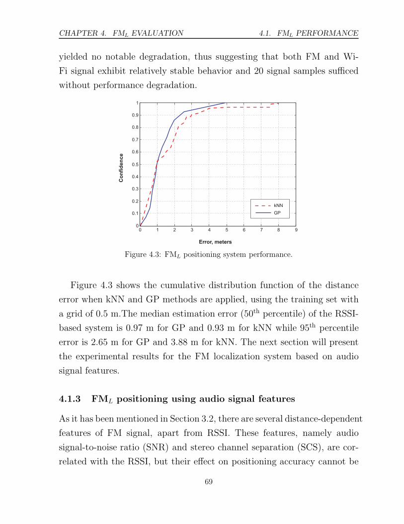
CHAPTER 4. FML EVALUATION 4.1. FML PERFORMANCE
yielded no notable degradation, thus suggesting that both FM and Wi-
Fi signal exhibit relatively stable behavior and 20 signal samples sufficed
without performance degradation.
Figure 4.3: FML positioning system performance.
Figure 4.3 shows the cumulative distribution function of the distance
error when kNN and GP methods are applied, using the training set with
a grid of 0.5 m.The median estimation error (50th percentile) of the RSSI-
based system is 0.97 m for GP and 0.93 m for kNN while 95th percentile
error is 2.65 m for GP and 3.88 m for kNN. The next section will present
the experimental results for the FM localization system based on audio
signal features.
4.1.3 FML positioning using audio signal features
As it has been mentioned in Section 3.2, there are several distance-dependent
features of FM signal, apart from RSSI. These features, namely audio
signal-to-noise ratio (SNR) and stereo channel separation (SCS), are cor-
related with the RSSI, but their effect on positioning accuracy cannot be
69

4.1. FML PERFORMANCE CHAPTER 4. FML EVALUATION
directly inferred. This section provides an experimental evaluation of the
positioning accuracy of an FML positioning system based on audio SNR
and stereo channel separation.
The experiment has been conducted in the testbed described in the
previous section. The beacons were set to transmit a stereophonic audio
signal; each stereo channel contained a sinusoidal signal of specific fre-
quency. The frequencies were selected so that the sine waves from different
channels, nor their harmonics, did not overlap. This has been achieved by
employing a DTMF signal [109]: 1209 Hz for the left channel, and 697 Hz
for the right one (these correspond to DTMF signal for “1”). At the client
side, there was a laptop computer equipped with a Brando USB FM Ra-
dio receiver [110]. For each accessible point of a 1 m grid in the testbed,
the client recorded a 5 s long audio sample from each beacon (44100 Hz
sampling frequency, stereo) and simultaneously acquired the RSSI values
for the beacon being recorded (the RSSI was sampled every 100 ms).
The recorded audio samples were processed to estimate the SNR and
channel separation values. The procedure was the following. Firstly, the
right channel data was discarded and only left channel data has been used
for processing. Then, the spectrum of left channel signal was evaluated by
fast fourier transform (FFT) with Hanning window of length 8192. The
signal magnitude was the magnitude of 1209 Hz band, as 1209 Hz signal
was the one actually transmitted in the left channel. The 697 Hz band, in
turn, represented the magnitude of the right-channel signal leaked into the
left one due to channel cross-talk. Thus, the stereo channel separation was
evaluated as the difference between 1209 Hz and 697 Hz band magnitudes.
The SNR was evaluated as the ratio of 1209 Hz band magnitude to the
average magnitude of all the other bands. Finally, the SNR, RSSI and
channel separation measurements for each point were averaged.
The evaluation of the positioning accuracy for each method has been
70

CHAPTER 4. FML EVALUATION 4.1. FML PERFORMANCE
performed using a kNN classifier (k = 1) and leave-one-out approach,
implemented in R language [111]. The results are presented in Figure 4.4.
Figure 4.4: Accuracy of FM positioning system using audio signal features.
The results confirm the feasibility of FM positioning based on audio sig-
nal properties, as all methods perform better than the baseline (where the
system returned a random training point for any input fingerprint). The
SCS approach demonstrates a slightly better performance than the SNR
one, and provides the best median accuracy of 2.1 m over all competitors.
However, the best overall accuracy is demonstrated by the RSSI approach.
In order to understand the reasons behind the inferior performance of
audio-based approaches, let us analyze the dependencies between the col-
lected SNR, SCS and RSSI values, presented in Figure 4.5.
Figure 4.5a shows the relationship between SNR and RSSI. As one can
see, for low RSSI values the SNR increases linearly or quasi-linearly. At a
certain point, however, the SNR reaches its maximum of about 50 dB and
saturates. This means that the SNR approach is usable for positioning only
71

4.1. FML PERFORMANCE CHAPTER 4. FML EVALUATION
(a) SNR vs. RSSI (b) SCS vs. RSSI
Figure 4.5: Relationship between SNR, SCS and RSSI.
at relatively long distances. At shorter range, when the signal strength is
high, the SNR’s dependence on distance is weak. This explains why SNR
demonstrated lower positioning accuracy than SCS: the power of the used
transmitters was sufficient to provide the good audio quality in most parts
of the test environment.
Figure 4.5b demonstrates the dependence of channel separation from
RSSI. When the signal is weak, the reception is monophonic and the chan-
nel separation is low. As the RSSI increases, the receiver eventually picks
up the stereo pilot tone and switches to stereophonic mode; the channel
separation improves with the further growth of the RSSI.
The experimental results demonstrate that SNR and SCS approaches
are more limited than the RSSI one. SCS works at shorter distances with
high RSSI values, while the SNR approach is more suitable at longer ranges
with low RSSI values. While SNR and SCS methods can be used for posi-
tioning, the RSSI is applicable for all ranges and provides better accuracy.
Therefore, all further experiments focus on the RSSI approach.
72

CHAPTER 4. FML EVALUATION 4.1. FML PERFORMANCE
4.1.4 Comparison of FML and Wi-Fi positioning accuracy
In order to understand how FM performance relates to other techniques,
and to ensure a fair comparison, another set of experiments has been per-
formed to evaluate the FM and Wi-Fi positioning systems performance in
the same testbed. As previously mentioned in Chapter 2, Wi-Fi localiza-
tion systems have gained a notable popularity due to the availability of
Wi-Fi infrastructure in many office buildings. This motivated the choice
of Wi-Fi as the localization technology to compare FM with.
(a) kNN (b) GP
Figure 4.6: FM versus Wi-Fi positioning system.
Figure 4.6 demonstrates the error distance CDFs for Wi-Fi and FM po-
sitioning systems utilizing two machine learning algorithms, namely kNN
and GP. As mentioned in Section 4.1.2, the test device (HTC Artemis) re-
ported Wi-Fi RSSI in a coarse-grained manner due to firmware limitations.
To ensure fair comparison of the two methods, the FM signal strengths were
mapped to a scale similar to Wi-Fi (see Table 4.1). Under these conditions,
Wi-Fi and FM systems demonstrate very similar performance (Figure 4.6).
From the comparison of the two graphs, one can note that the classi-
fication approach provides slightly better median accuracy, but it is more
prone to distant outliers, which increase the error for high confidence levels.
73

4.1. FML PERFORMANCE CHAPTER 4. FML EVALUATION
The regression approach, in contrast, is more suitable for applications that
require high reliability of position information. Also, it should be noted
that the nature of classification method makes it impossible for kNN to
provide any estimation with an error smaller than the dimension of used
grid (in this experiment it was 1 m) while this is not the case for GP
regression.
4.1.5 Performance of a combined FML and Wi-Fi system
In the literature, there are a number of reports demonstrating that the
positioning systems which perform a fusion of different localization tech-
nologies usually provide better accuracy than any of these technologies in
isolation [10, 43, 112]. This section presents the performance results of a
system combining FM and Wi-Fi fingerprinting.
The data fusion has been done by merging the FM and Wi-Fi finger-
prints into wider FM+Wi-Fi fingerprints. Despite the simplicity of such
data fusion approach, it has been previously demonstrated as being capa-
ble to provide an improved localization performance [50, 51, 72]. In this
experiment, each wide fingerprint included 6 RSSI values: 3 for FM and 3
for Wi-Fi. The FM RSSI values were of full precision, without conversion
to the 6-level values.
The localization accuracy of the combined FM+Wi-Fi system is pre-
sented in Figure 4.7. For both data processing methods, the combined
system outperforms each of the underlying technologies alone. While for
GP the difference is minor, in the case of kNN even low-precision Wi-Fi
fingerprints can significantly improve the positioning accuracy of pure-FM
approach. The fusion of FM and Wi-Fi positioning technologies improved
the positioning accuracy by up to 22% (0.85 m at 95th percentile for kNN).
Combining Wi-Fi and FM positioning systems also has a number of
other advantages. In the environments with existing Wi-Fi infrastruc-
74
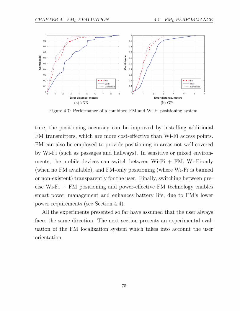
CHAPTER 4. FML EVALUATION 4.1. FML PERFORMANCE
(a) kNN (b) GP
Figure 4.7: Performance of a combined FM and Wi-Fi positioning system.
ture, the positioning accuracy can be improved by installing additional
FM transmitters, which are more cost-effective than Wi-Fi access points.
FM can also be employed to provide positioning in areas not well covered
by Wi-Fi (such as passages and hallways). In sensitive or mixed environ-
ments, the mobile devices can switch between Wi-Fi + FM, Wi-Fi-only
(when no FM available), and FM-only positioning (where Wi-Fi is banned
or non-existent) transparently for the user. Finally, switching between pre-
cise Wi-Fi + FM positioning and power-effective FM technology enables
smart power management and enhances battery life, due to FM’s lower
power requirements (see Section 4.4).
All the experiments presented so far have assumed that the user always
faces the same direction. The next section presents an experimental eval-
uation of the FM localization system which takes into account the user
orientation.
75

4.2. RECOGNITION OF ORIENTATION CHAPTER 4. FML EVALUATION
4.2 Recognition of orientation
The orientation of a user might have a significant impact on the observed
signal strength and consequently on the localization accuracy. The reasons
for that lie in the direction of mobile unit’s antenna, reflections of the radio
signals and the fact that components of the mobile unit can partly shield
signals from certain directions [113]. For Wi-Fi signals, the user body
has a noticeable effect on the signal strength variations [20, 107]. This is
explained by the fact that a human body is 70% composed of water and that
the resonant frequency of water is 2.4 GHz (similar to Wi-Fi frequencies),
which ultimately results in the attenuation of Wi-Fi radio signals by up
to 9 dB [107] due to human body. Thus, changing the direction of the
mobile device will result in the change of the RSS, even if the position
remains fixed. The RADAR project [20] investigated the case in which the
training set points were acquired while facing a single direction, while the
test samples corresponded to the other three directions. In this case, their
results showed a significant (up to 67%) degradation of the localization
accuracy.
However, the frequencies of FM radio signals are by orders of magnitude
less than the resonant frequency of water, and the effect of user body orien-
tation on the positioning accuracy can be different from Wi-Fi results. The
following sections will examine the accuracy of the FML positioning sys-
tem considering the orientation, and test whether the orientation-induced
changes in RSS can provide means for detecting user’s facing direction.
4.2.1 Impact of orientation on positioning accuracy
This section considers two possible solutions for overcoming the problem
of user orientation affecting the RSS fingerprints.
• The first solution consists of having four different training sets (one
76
CHAPTER 4. FML EVALUATION 4.2. RECOGNITION OF ORIENTATION
for each orientation). To estimate the location, one of these sets would
be used depending on the user’s orientation at any given time. The
current orientation would be detected using an additional sensor, such
as a compass.
• The second solution is based on using one extensive training set that
is composed of signal strengths from the three FM beacons for all four
orientations in each physical point.
These two approaches have been tested experimentally in order to verify
whether having an additional sensor for orientation is an acceptable trade-
off in terms of localization accuracy.
The RSSI measurements have been performed in 40 physically accessible
points in the testbed, following a 1-meter grid (Figure 4.1). In each point,
20 samples were taken for all four directions: facing North, South, East and
West. This resulted in four training sets, one for each direction. The first
approach assumes that the orientation is known, so to estimate the user’s
position one of the four training sets is used accordingly. The accuracy for
each orientation has been evaluated by applying the leave-one-out method
on four training datasets separately (North, South, East and West graphs
in Figure 4.8). Note that the mobile device may be oriented in between
of two orientations, such as between North and West for example. In this
case, the closest of the four orientations should be taken as the actual user’s
orientation and the corresponding training set should be used. This means
that 45◦is the maximal error, which, according to the experimental results,
does not significantly affect the RSSI.
In order to compare this approach with the second solution, a leave-one-
out evaluation has been performed on the dataset composed of previously
used four datasets containing North, South, East and West orientations,
all merged together. For each physical point, the leave-one-out method
77

4.2. RECOGNITION OF ORIENTATION CHAPTER 4. FML EVALUATION
(a) kNN
(b) GP
Figure 4.8: Positioning accuracy depending on orientation.
78
CHAPTER 4. FML EVALUATION 4.2. RECOGNITION OF ORIENTATION
excludes from the training set all the measurements (for all orientations)
that belong to the current point, and assigns all the other samples (for
all four orientations) to the training set. The results are presented in
Figure 4.8 for both kNN and GP localization methods.
From the obtained results it can be seen that one extensive training
set containing measurements for all four orientations provides a similar
localization accuracy to the case when the orientation is known and the
corresponding training set is used. In particular, the graphs show that the
localization accuracy of using the merged training set with four orientations
is very similar to the result of fixed orientation training sets West and East
for kNN and North and West for GP (Figure 4.8).
Intuitively, a number of different fingerprints associated to one physical
point would result in decreased localization accuracy, since the probability
of having similar fingerprints in two or more physical points is higher (for
example, facing North in one point may produce the same fingerprint as
facingWest in another point). Despite this intuition, however, the accuracy
of the FM localization system degrades negligibly even if the calibration
set includes fingerprints for all orientations. This may be attributed to
relatively small interaction of human body with the FM-band radio waves,
in comparison to higher-frequency Wi-Fi signals.
Thus, the experimental results demonstrate that the impact of the user
body orientation on the FM localization accuracy is minimal, which pro-
vides a good basis for a real-life localization system.
4.2.2 Analysis of user’s orientation
Although the user body orientation has been shown to have a minor impact
on the localization accuracy, the RSSI readings are nevertheless affected by
the orientation. This motivated the investigation of whether it is possible
to recognize the user facing direction from the RSSI readings.
79
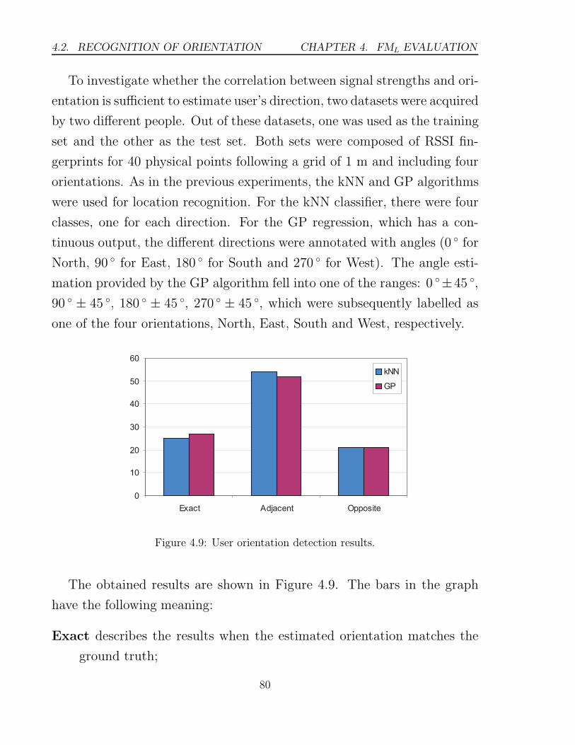
4.2. RECOGNITION OF ORIENTATION CHAPTER 4. FML EVALUATION
To investigate whether the correlation between signal strengths and ori-
entation is sufficient to estimate user’s direction, two datasets were acquired
by two different people. Out of these datasets, one was used as the training
set and the other as the test set. Both sets were composed of RSSI fin-
gerprints for 40 physical points following a grid of 1 m and including four
orientations. As in the previous experiments, the kNN and GP algorithms
were used for location recognition. For the kNN classifier, there were four
classes, one for each direction. For the GP regression, which has a con-
tinuous output, the different directions were annotated with angles (0 ◦ for
North, 90 ◦ for East, 180 ◦ for South and 270 ◦ for West). The angle esti-
mation provided by the GP algorithm fell into one of the ranges: 0 ◦±45 ◦,
90 ◦ ± 45 ◦, 180 ◦ ± 45 ◦, 270 ◦ ± 45 ◦, which were subsequently labelled as
one of the four orientations, North, East, South and West, respectively.
Figure 4.9: User orientation detection results.
The obtained results are shown in Figure 4.9. The bars in the graph
have the following meaning:
Exact describes the results when the estimated orientation matches the
ground truth;
80
CHAPTER 4. FML EVALUATION 4.3. ACCURACY DEGRADATION
Adjacent corresponds to the cases when the estimated and real orienta-
tion are adjacent (for example, when the system recognizes the true
West orientation as North);
Opposite depicts the cases when the estimated and real orientation have
opposite directions.
It can be seen that the results are similar to a random prediction: around
25% for the accurate estimation, around 50% for one of two adjacent ori-
entations and almost 25% for the opposite directions.
Therefore, the correlation between signal strengths and orientations
proved to be insufficient for detection of user body orientation in an FM
localization system. These results are in line with the literature reports for
Wi-Fi signals. Saha et al. [114] found that while the variation of Wi-Fi sig-
nal due to user direction were within 3–4 dB, this value was less than RSSI
variation across different locations and even below the RSSI fluctuations
within a fixed location (5–7 dB) [114]. Thus, both FM and Wi-Fi systems
cannot recognize user body orientation from localization RSSI fingerprints.
4.3 Accuracy degradation
Radio signal propagation in an indoor environment is affected by a number
of factors, both dynamic (people movement) and long-lasting (furniture
layout changes, atmosphere conditions). These factors can change the
propagation conditions so that the previously collected fingerprints differ
from the current ones, which might significantly decrease the localization
accuracy [103].
To evaluate the long-term stability of the FM localization, a number of
fingerprint datasets have been collected over the period of seven months,
from December 2008 till July 2009. Unexpectedly, the test that was per-
formed in July using the set of fingerprints measured in June showed more
81

4.3. ACCURACY DEGRADATION CHAPTER 4. FML EVALUATION
degradation in comparison to the tests in June and July using the training
set acquired in December. Such results point to a conclusion that finger-
print fluctuations are derived from a random process and are difficult to
predict. The following experiments consider the datasets with the highest
accuracy degradation (June and July 2009).
4.3.1 Lessening the causes of degradation
The first step of addressing the performance degradation is to lessen the
causes of degradation through preprocessing the input data. Some environ-
mental factors, such as air humidity, simultaneously affect the RSSI from
all beacons. To compensate for such changes, the RSSI readings from the
three FM transmitters have been represented as a matrix with columns
ss1, ss2, and ss3 and preprocessed in the following way. Firstly, the ab-
solute RSSI values were converted to their pairwise differences (ss1− ss2,
ss2−ss3, ss1−ss3). Then, each column was divided by its maximum value
and finally the resulting values were centered around zero by subtracting
each column’s mean value. The idea behind this procedure was to miti-
gate the RSSI changes over time and to make new inputs less dependent
on their absolute values.
The described preprocessing has improved the performance of the GP
regression (even for the same dataset, see Figure 4.10), but had an adverse
impact on kNN results and therefore was used only with GP.
Applying the GP regression to the preprocessed data proved the as-
sumption that all transmitters generally follow the same pattern of change
or exhibit same degradation levels and that the described preprocessing
procedure can mitigate the system degradation to a certain extent. As
a result, the median accuracy of the system trained on the June dataset
and tested on the July one, improved from 2 m to 1.45 m only due to
preprocessing (Figure 4.10).
82
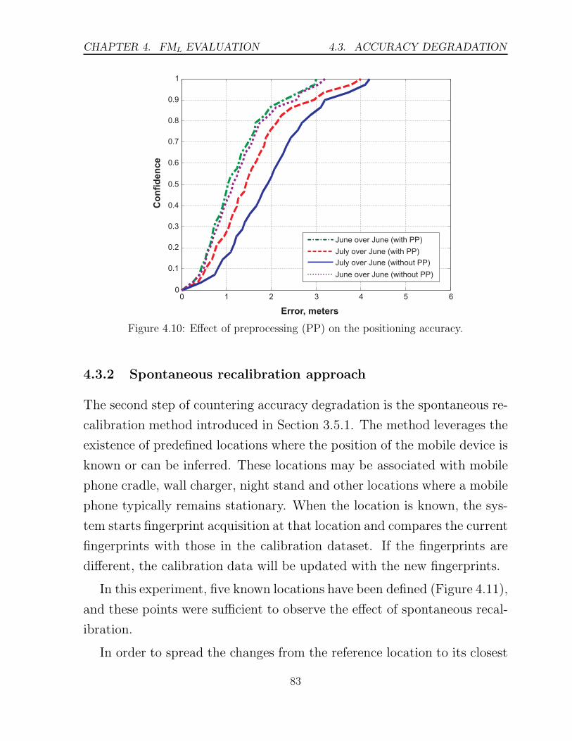
CHAPTER 4. FML EVALUATION 4.3. ACCURACY DEGRADATION
Figure 4.10: Effect of preprocessing (PP) on the positioning accuracy.
4.3.2 Spontaneous recalibration approach
The second step of countering accuracy degradation is the spontaneous re-
calibration method introduced in Section 3.5.1. The method leverages the
existence of predefined locations where the position of the mobile device is
known or can be inferred. These locations may be associated with mobile
phone cradle, wall charger, night stand and other locations where a mobile
phone typically remains stationary. When the location is known, the sys-
tem starts fingerprint acquisition at that location and compares the current
fingerprints with those in the calibration dataset. If the fingerprints are
different, the calibration data will be updated with the new fingerprints.
In this experiment, five known locations have been defined (Figure 4.11),
and these points were sufficient to observe the effect of spontaneous recal-
ibration.
In order to spread the changes from the reference location to its closest
83

4.3. ACCURACY DEGRADATION CHAPTER 4. FML EVALUATION
Figure 4.11: Positions of the points used for spontaneous recalibration.
neighboring points, a propagation model has been employed (Formula 3.5
in Section 3.5.1). The parameters of the model have been found empirically
from the initial training set. The best suited value for the path loss change
rate n was 2, while the wall attenuation factor was set to zero, as there were
no walls between adjacent points. For each reference point, eight neighbor-
ing points have been adjusted using the propagation model. Thus, 45 out
of 140 points were updated (5 reference locations plus 5 × 8 neighboring
points). As a result, the spontaneous recalibration further improved the
median localization accuracy from 1.45 m to 1.2 m (Figure 4.12a).
(a) Using separate training and testing sets (b) Using leave-one-out approach
Figure 4.12: Effect of the spontaneous recalibration on system performance.
84
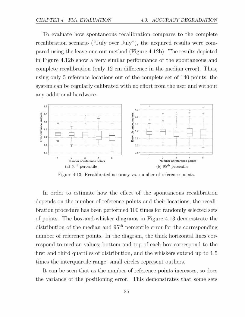
CHAPTER 4. FML EVALUATION 4.3. ACCURACY DEGRADATION
To evaluate how spontaneous recalibration compares to the complete
recalibration scenario (“July over July”), the acquired results were com-
pared using the leave-one-out method (Figure 4.12b). The results depicted
in Figure 4.12b show a very similar performance of the spontaneous and
complete recalibration (only 12 cm difference in the median error). Thus,
using only 5 reference locations out of the complete set of 140 points, the
system can be regularly calibrated with no effort from the user and without
any additional hardware.
(a) 50th percentile (b) 95th percentile
Figure 4.13: Recalibrated accuracy vs. number of reference points.
In order to estimate how the effect of the spontaneous recalibration
depends on the number of reference points and their locations, the recali-
bration procedure has been performed 100 times for randomly selected sets
of points. The box-and-whisker diagrams in Figure 4.13 demonstrate the
distribution of the median and 95th percentile error for the corresponding
number of reference points. In the diagram, the thick horizontal lines cor-
respond to median values; bottom and top of each box correspond to the
first and third quartiles of distribution, and the whiskers extend up to 1.5
times the interquartile range; small circles represent outliers.
It can be seen that as the number of reference points increases, so does
the variance of the positioning error. This demonstrates that some sets
85

4.4. POWER CONSUMPTION ANALYSIS CHAPTER 4. FML EVALUATION
of reference positions are more effective than the others, and by carefully
selecting the reference points it is possible to significantly reduce the ac-
curacy degradation. The graphs also show that the accuracy of a recali-
brated system generally improves as the number of reference points grows.
As explained above, the accuracy gain can be further increased by careful
selection of the reference locations.
4.4 Analysis of FM and Wi-Fi power consumption
This section provides a theoretical and experimental comparison of FM
and Wi-Fi power consumption.
Unlike Wi-Fi modules, the FM tuners are designed for receiving signals
and cannot transmit them. Moreover, Wi-Fi requires complicated data pro-
cessing, while FM demodulation is rather straight-forward process. Due to
these two facts, FM receivers have considerably lower power consumption
than Wi-Fi modules. Depending on the complexity of its circuitry, an FM
receiver can consume from about 15 mW (TDA7088 [94], analog–only) to
about 50 mW (Si4703 [77] with RDS enabled). In contrast, Anand et al.
[47] have reported idle-state Wi-Fi power consumption varying from 190–
390 mW in power-saving mode to 1200 mW in constantly-active mode.
Evidently, FM tuners are significantly more power-effective than Wi-Fi
network modules. However, the runtime of a mobile device also depends
on other components (such as CPU and display) and CPU load. Therefore,
it is more appropriate to measure the total battery life of the device, rather
than the consumption of separate components.
The battery life tests were carried out using a Samsung Omnia 2 smart-
phone running My Experience tool [115] with FM and Wi-Fi fingerprinting
sensors. My Experience is a popular platform for acquisition of user experi-
ence data, which often includes location. Thus, the experiment simulated
86

CHAPTER 4. FML EVALUATION 4.4. POWER CONSUMPTION ANALYSIS
one of the real applications for a positioning system. During the tests,
My Experience periodically acquired location fingerprint and stored it in a
database; the device was kept in the “unattended” power state [116], with
screen and backlight turned off. All tests started with a completely charged
battery and continued until the device run out of power and switched off.
The running time was then extracted from My Experience logs.
Two groups of tests have been performed, separately for Wi-Fi and FM.
In order to minimize the influence of other components, all unused wireless
modules were switched off (GSM and Bluetooth — for all tests, Wi-Fi
— during FM tests, and FM — during Wi-Fi tests). The modules were
configured for localization purposes in the following way. For FM tests, a
standard headset was connected to the device to serve as an FM antenna;
Wi-Fi module was switched off; sound volume was set to zero. During
Wi-Fi tests, FM was switched off; Wi-Fi network card was not associated
with any nearby access points, to ensure that there are no background data
transfers. Both modules used the available power saving routines.
The FM-related tests took into account the number of beacons in fin-
gerprint. While for Wi-Fi the fingerprint acquisition time of 1 s was rela-
tively constant and independent on the number of beacons, an FM receiver
needed to switch from one beacon to another explicitly. Thus, wider FM
fingerprints imply longer duty cycles due to increased channel switching
and longer sample acquisition times; this potentially leads to higher power
consumption. FM sample acquisition times are presented in Table 4.2.
Table 4.2: FM RSSI sample acquisition time for different fingerprint width.
Beacons in fingerprint Acquisition time, s3 0.410 1.545 9.0205 36
87

4.4. POWER CONSUMPTION ANALYSIS CHAPTER 4. FML EVALUATION
Figure 4.14: Battery life in FM and Wi-Fi fingerprinting modes. The baseline correspondsto all wireless modules switched off.
Figure 4.14 presents the results of battery life measurements in FM
and Wi-Fi fingerprinting modes for different scan intervals. As expected,
the run time of the device grows as the time interval between scans in-
creases.Unfortunately, it was impossible to evaluate Wi-Fi performance
with 1 s update period, as the Wi-Fi driver was unstable at high sampling
rates and quickly crashed. From the general trend, however, it is evident
that the result would have been less than 7.4 h, which is still significantly
below the 27.9 h demonstrated by FM with 3 beacons. Overall, FM demon-
strates superior power efficiency, providing 2.6 to 5.5 times longer battery
life than Wi-Fi and closely approaching the baseline maximum.
88

CHAPTER 4. FML EVALUATION 4.5. SUMMARY
4.5 Summary
The evaluation presented in this chapter demonstrated the possibility of in-
door localization using signals of local short-range FM transmitters. Both
RF signal strength and audio signal characteristics, such as signal-to-noise
ratio (SNR) and stereo channel separation (SCS) can be used for position-
ing. It has been found, however, that SCS method works only at short
distances from transmitters while the SNR one — only at longer distances.
The RSSI, in turn, covers the whole range and provides superior positioning
accuracy.
FML provided similar accuracy to the Wi-Fi localization system in-
stalled in the same environment; the median error for FML was 0.9 m in a
50m2 room. It has been demonstrated that combination with FML can im-
prove performance of an existing Wi-Fi positioning system. The two data
analysis approaches used, classification (kNN) and regression (Gaussian
processes), demonstrated better median accuracy for classification, but re-
gression has faster convergence and excelled at high confidence levels. The
experiments on direction recognition have shown that RSSI is affected by
the user orientation. However, the accuracy of direction recognition us-
ing RSSI fingerprints was indistinguishable from random. The positive
result was that user orientation had only minimal impact on localization
accuracy.
This chapter also demonstrated that the gradual degradation of accu-
racy, which is inherent to any fingerprinting based system, can be countered
by fingerprint preprocessing and spontaneous recalibration. The latter is
capable of periodical updating the calibration dataset transparently to the
user and without any additional hardware.
Finally, the power consumption tests have shown that FM fingerprinting
is significantly more power-efficient than Wi-Fi. Depending on sampling
89

4.5. SUMMARY CHAPTER 4. FML EVALUATION
rate and number of scanned beacons, the mobile device with FM position-
ing client provides 2.6 to 5.5 times longer battery life than in the case of
Wi-Fi localization, closely approaching the device’s maximum run time.
90

Chapter 5
Evaluation of FM positioning using
broadcasting stations (FMB)
This chapter presents the results of experimental evaluation of indoor po-
sitioning based on broadcasting FM stations (FMB), the comparison with
other positioning systems, such as Wi-Fi and GSM. Also, an experimental
evaluation of FMB RSSI stability and its dependence on people’s presence
is provided.
5.1 Detection of active broadcasting stations
In Europe, the FM band spans from 87.5 to 108.0 MHz with 100 kHz
channel spacing. This results in 205 FM channels. While there are many
FM stations, usually not all of the available channels are utilized. Clearly, it
makes little sense for FM positioning to consider inactive channels without
transmission, as they introduce additional noise into fingerprints, increase
scanning time and storage requirements. Therefore, there is a need for a
method capable of detecting the channels with active transmission.
The common method of finding active broadcasting stations during seek
tuning, employed by virtually all FM receivers, is RSSI thresholding, where
the receiver registers a broadcasting station at a specific channel if its RSSI
91

5.1. ACTIVE STATION DETECTION CHAPTER 5. FMB EVALUATION
level is above the predefined threshold [77, 94, 117]. While this approach
is widely used due to its simplicity, it is not very robust, as setting the
threshold too low would increase the number of false-positive detections.
On the other hand, with a too high threshold the receiver may not rec-
ognize less powerful stations. The manufacturers of FM receiver solutions
address this problem by introducing additional channel validation criteria,
such as peak noise detectors [77] and SNR estimates [117, 118], interme-
diate frequency checks [119, 120]. These measures significantly decrease
the number of false channel detections. Unfortunately, in some cases the
additional seek tuning qualifiers are not available, either due to hardware
limitations or when the channel activity data has not been recorded.
In order to evaluate the possibility of detecting active FM channels using
only RSSI data, the following experiment has been performed. Initially,
the list of active channels has been acquired using the receiver’s hardware
seek tuning functionality. The receiver was Brando USB FM radio (based
on Si4700 chip [121]), the channel spacing was set to 100 kHz and the RSSI
threshold was set to 15/63. The procedure was repeated three times and
the channels detected in all three cases were listed. Totally, 54 channels
have been detected; 7 of them had very high level of audio noise. At the
next step, the whole FM band was scanned three times and mean RSSI
values for each channel were recorded. The acquired data is presented in
Figure 5.1.
According to the results, the assumption that active stations correspond
to peaks on RSSI graph, is not valid. Instead, the active stations usually
appear within 100 kHz from the peaks, which are produced by additive
interference of adjacent channels (see, for example, 91.6 MHz in Figure 5.1).
Such cases are usually associated with a sharp increase of the RSSI. If there
was no sharp increase of the RSSI, then the station is probably associated
with the peak. Finally, all the active stations found by seek tuning have
92
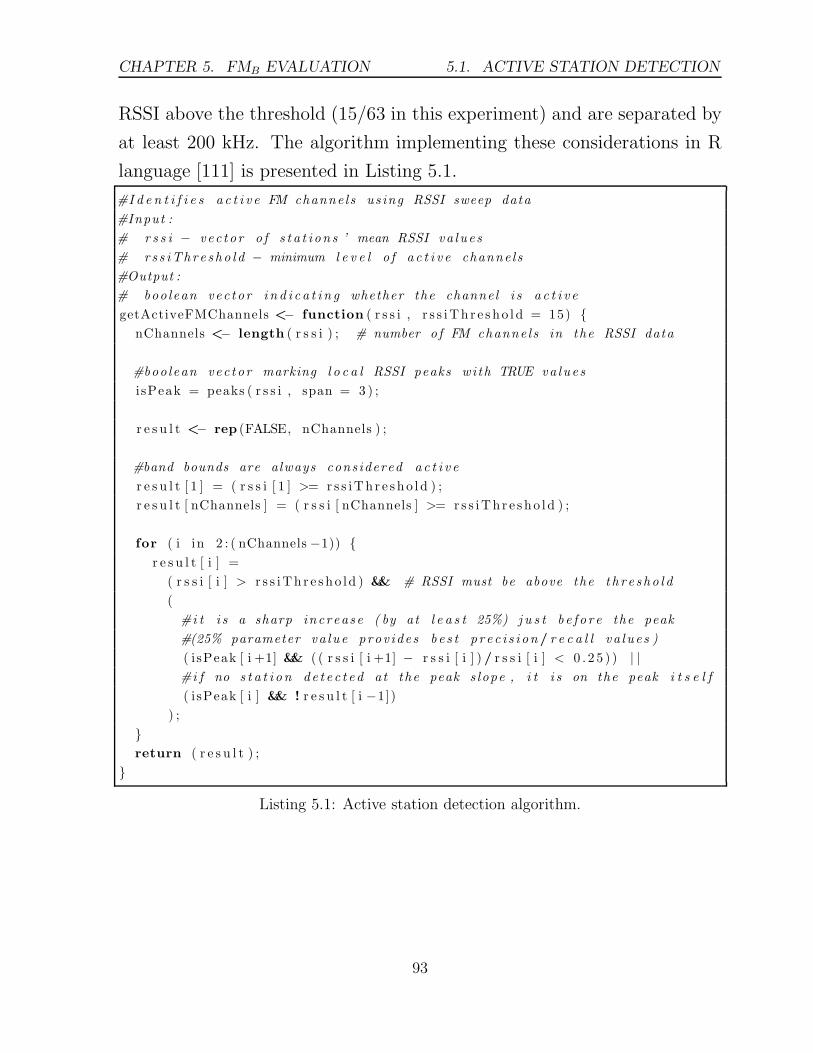
CHAPTER 5. FMB EVALUATION 5.1. ACTIVE STATION DETECTION
RSSI above the threshold (15/63 in this experiment) and are separated by
at least 200 kHz. The algorithm implementing these considerations in R
language [111] is presented in Listing 5.1.
#I d e n t i f i e s a c t i v e FM channe l s us ing RSSI sweep data
#Input :
# r s s i − vec t or o f s t a t i on s ’ mean RSSI va lu e s
# r s s iThr e s ho l d − minimum l e v e l o f a c t i v e channe l s
#Output :
# boolean vec t or i n d i c a t i n g whether the channel i s a c t i v e
getActiveFMChannels <− function ( r s s i , r s s iTh r e s ho l d = 15) {
nChannels <− length ( r s s i ) ; # number o f FM channe l s in the RSSI data
#boolean vec t or marking l o c a l RSSI peaks wi th TRUE va lues
i sPeak = peaks ( r s s i , span = 3 ) ;
r e s u l t <− rep (FALSE, nChannels ) ;
#band bounds are always cons idered a c t i v e
r e s u l t [ 1 ] = ( r s s i [ 1 ] >= r s s iTh r e s ho l d ) ;
r e s u l t [ nChannels ] = ( r s s i [ nChannels ] >= r s s iTh r e s ho l d ) ;
for ( i in 2 : ( nChannels −1)) {
r e s u l t [ i ] =
( r s s i [ i ] > r s s iTh r e s ho ld ) && # RSSI must be above the t h r e s ho l d
(
#i t i s a sharp increase ( by at l e a s t 25%) j u s t b e f o r e the peak
#(25% parameter va lu e prov ide s b e s t p r e c i s i on / r e c a l l va lu e s )
( isPeak [ i +1] && ( ( r s s i [ i +1] − r s s i [ i ] ) / r s s i [ i ] < 0 . 2 5 ) ) | |
#i f no s t a t i o n de t e c t e d at the peak s lope , i t i s on the peak i t s e l f
( isPeak [ i ] && ! r e s u l t [ i −1])
) ;
}
return ( r e s u l t ) ;
}
Listing 5.1: Active station detection algorithm.
93
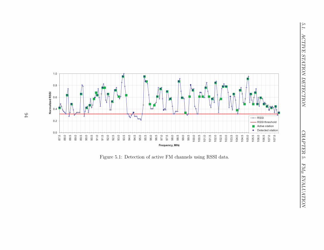
5.1.
ACTIV
ESTATIO
NDETECTIO
NCHAPTER
5.
FM
BEVALUATIO
N
Figure 5.1: Detection of active FM channels using RSSI data.
94
CHAPTER 5. FMB EVALUATION 5.2. FMB PERFORMANCE
The results of active channel detection using RSSI data are presented
in Figure 5.1. The algorithm found 45 active channels, with 80% precision
and 67% recall with regard to the 54 channels found by seek tuning. For
the FM positioning, it is more important to minimize the number of false
positive detections rather than false negatives; in other words, it is better
to miss some active stations rather than rely on high-power noise. The 80%
precision demonstrated by the presented algorithm provides a suitable basis
for identification of active FM channels using only RSSI data.
5.2 FMB positioning system performance
This section provides performance evaluation results of the positioning
system using RSSI fingerprints of broadcasting FM stations.
The experimental environment was the same as in the FML positioning
experiments (Figure 4.1 in Chapter 4). The furniture layout, however, has
changed since then, which changed the spatial distribution of RSSI and
also influenced the positioning accuracy results. Due to these changes, the
FML results presented in this section are different from the FML results
previously reported in Section 4.1.2.
Before the measurements, the list of active FM channels was acquired at
several parts of the room using Brando USB FM receiver’s “seek tuning”
capability (RSSI threshold was set to 15/63). All detected channels were
combined into a single list of 76 active FM stations. Three local FM
transmitters were installed at the locations shown in Figure 4.1 and tuned
to transmit DTMF “1” signal at frequencies not occupied by broadcasting
stations.
FM fingerprints were acquired by Samsung Omnia 2 smartphone. The
RSSI values were collected at the points defined by a 1 m grid; due to the
furniture, totally 40 points have been measured in the 12×6 m room. The
95

5.2. FMB PERFORMANCE CHAPTER 5. FMB EVALUATION
experimenter was always facing the same direction. Each FM fingerprint
included 10 RSSI samples of each of 79 channels (76 broadcasting stations
and 3 local transmitters).
The preprocessing step comprised normalization of the fingerprints’ RSSI
values to 0..1 range in accordance with the characteristics of the corre-
sponding receivers (Appendix B.1). To recognize locations by fingerprints,
a k-nearest neighbour classifier (k = 1) has been used (see Section 3.4).
The positioning performance was evaluated using leave-one-out approach
(Section 3.4.3).
Figure 5.2: FMB and FML positioning accuracy.
The performance results of the FMB positioning system using all broad-
casting FM stations are presented in Figure 5.2 (local beacons are ex-
cluded). The median positioning error of the system is 0.91 m, the 95th
percentile error is 4.71 m. For confidence levels of up to 90%, FMB out-
performs the FML positioning based on three local beacons. Evidently,
such a high FMB performance should be attributed to the high number of
96

CHAPTER 5. FMB EVALUATION 5.2. FMB PERFORMANCE
used beacons: there is evidence in the literature that suggests that wider
fingerprints result in better positioning performance [2, 50, 51, 72].
5.2.1 Accuracy vs. number of beacons
In the previous section, all the beacons have been used for positioning.
However, wide fingerprints take more time to acquire and increase the
dimensionality of the classification task, thus increasing the computational
requirements of the positioning system. Therefore, it would be beneficial
to find a trade-off between the fingerprint width and localization accuracy,
assuming that not all of the beacons contribute to positioning equally.
Indeed, if the character of obstacles between the test environment and
certain broadcasting stations is the same for the majority of test points,
the signal properties from such station are likely to remain the same for the
large part of the environment and such a station can be safely excluded.
This section describes a number of FMB beacon selection approaches and
evaluates how number of beacons (fingerprint width) affects the positioning
accuracy.
One of the most obvious, although rather naıve, methods is to select the
stations with highest signal strength, which comes along with the inverse
approach of preferring the stations with low RSSI values. The results for
these approaches are presented in Figure 5.3. As one can see, the two
methods have similar performance in terms of median error (Figure 5.3a).
For higher confidence levels, the results are inconsistent: sometimes weaker
stations perform worse (at 67%), sometimes better (at 95%). The unstable
performance of strong stations at 95% confidence (Figure 5.3c) can be
explained by increased variation of the high RSSI levels, which results in
few points with high positioning error, which, in turn, significantly affect
the high-confidence positioning performance.
The presented findings are in contradiction with the results previously
97
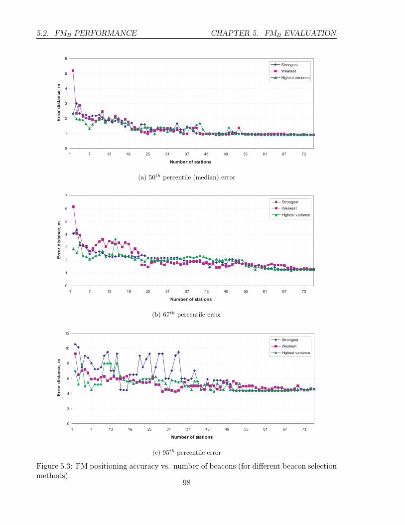
5.2. FMB PERFORMANCE CHAPTER 5. FMB EVALUATION
(a) 50th percentile (median) error
(b) 67th percentile error
(c) 95th percentile error
Figure 5.3: FM positioning accuracy vs. number of beacons (for different beacon selectionmethods).
98

CHAPTER 5. FMB EVALUATION 5.2. FMB PERFORMANCE
Figure 5.4: RSSI difference caused by path loss at indoor and outdoor scales.
demonstrated for outdoors. Fang et al. [2] have found that in outdoor
scenarios selecting stations with stronger signals leads to better position-
ing accuracy than for weak-signal stations [2, Fig. 4]. To understand the
reasons of this inconsistency, let us consider the difference between indoor
and outdoor positioning using broadcasting beacons. In outdoor scenario,
the distances between test points are relatively large (100–150 m in [2]).
At such distances, the signals of nearby (strong-signal) stations are subject
to significant path loss (see Section 2.1.4.1). In indoor environments, the
distances between test points are by orders of magnitude smaller (1 m in
Section 5.2), and path loss has minimal effect on signal propagation (see
Figure 5.4). In this case, the FM signal RSSI varies between indoor loca-
tions mainly due to walls and other obstacles, which equally affect all bea-
cons transmitting from the same direction, despite their signal strengths.
99

5.2. FMB PERFORMANCE CHAPTER 5. FMB EVALUATION
Therefore, in indoor scenarios stronger stations have no advantage over
weaker ones in terms of positioning performance.
As the results suggest, the averaged signal strengths of individual sta-
tions are not a good indication of their contribution to positioning per-
formance. Instead, the suitability of each station should be estimated by
taking into account the properties of the test environment. The third ap-
proach considers this by selecting the stations with the most diverse signals
across the test points. In particular, it evaluates the standard deviation
of signals from a beacon using averaged fingerprints of every test point. It
can be argued, that a high signal diversity might be caused by external
interfering factors rather than by the location of test points. Nevertheless,
the described approach outperforms the strongest/weakest station methods
for small number of beacons (see Figure 5.3). As the number of beacons
increases, the accuracy of this approach becomes similar to the others,
possibly due to the external interference mentioned above.
Figure 5.5: FMB positioning using 7 beacons with highest signal diversity.
The “highest diversity” graphs in Figure 5.3 have an evident local min-
100

CHAPTER 5. FMB EVALUATION 5.2. FMB PERFORMANCE
imum at 7 stations, for which the accuracy of the system is only slightly
inferior to that with all 76 beacons. Figure 5.5 confirms that the median
error of a system using only 10% of all beacons is 1.3 m, or only 0.4 m
worse than that of the full-scale system.
The presented results confirm that careful selection of broadcasting FM
beacons can reduce the fingerprint width by 90% with only minor degra-
dation of positioning accuracy.
5.2.2 Comparison of FMB and Wi-Fi positioning accuracy
This section provides a comparison of experimental results of FMB po-
sitioning performance and that of Wi-Fi, which is the current de-facto
standard of indoor localization.
The Wi-Fi fingerprints were collected with Samsung Omnia 2 device,
simultaneously with the FM data, as described in Section 5.2. 10 Wi-Fi
samples were acquired at each point with 1 s interval. Totally, there were
17 different Wi-Fi beacons in the dataset (many of them only at certain
points). The collected RSSI values were normalized to 0..1 range according
to the device specifications (Appendix B.1).
For classification was used the same kNN (k = 1) method as in the
FMB case. The beacons missing in particular fingerprints, were marked by
not-a-number (NaN) RSSI values and were ignored by the kNN. So, the
distance between fingerprints was evaluated using information only about
the beacons present in the test fingerprint. The classification accuracy was
evaluated using leave-one-out method.
The results are presented in Figure 5.6. The median error for the Wi-Fi
system is 1.6 m (versus 0.9 m for FMB) and in all cases the positioning
accuracy is within 4.5 m (6.0 m for FMB). As shown in the graph, FMB
outperforms Wi-Fi system for confidence levels of up to 90%. This can be
explained by the significantly higher number of FMB beacons (76 versus
101

5.2. FMB PERFORMANCE CHAPTER 5. FMB EVALUATION
Figure 5.6: FMB and Wi-Fi positioning accuracy using all beacons (76 and 17, respec-tively).
17 of Wi-Fi). On the other hand, all Wi-Fi beacons are installed in the
same building and are less affected by external interference sources.
5.2.3 Performance of a combined FMB and Wi-Fi system
In the related work, it has been demonstrated that a fusion of different
positioning methods can result in better positioning performance [43, 112,
122]. This section evaluates the performance of a combined FMB and Wi-
Fi positioning system.
A simple data fusion approach has been used to combine the two sys-
tems, where the FMB fingerprints acquired in previously described experi-
ments were widened with Wi-Fi fingerprints. A normalization of the RSSI
values according to specifications of the appropriate wireless module has
been performed to ensure balanced contribution of both technologies. It
should be noted, however, that the imbalance caused by different width
of the original fingerprints was not addressed, and the system with wider
102

CHAPTER 5. FMB EVALUATION 5.2. FMB PERFORMANCE
fingerprints influenced the similarity evaluation to a larger extent.
(a) Using all 76 FMB and all 17 Wi-Fi beacons
(b) Using 7 best FMB and all 17 Wi-Fi beacons
Figure 5.7: Combined FMB and Wi-Fi positioning accuracy .
Figure 5.7 provides the comparison of standalone and combined sys-
tem for the case when all FMB beacons are used and a more practical
103
5.2. FMB PERFORMANCE CHAPTER 5. FMB EVALUATION
option, when only a subset of beacons is employed (the selection criteria
are described in Section 5.2). In both cases, the combined system slightly
outperforms the standalone ones, except for the 100% confidence level,
where Wi-Fi dominates. In practical use, when absolute accuracy is not
required, the combined FMB+Wi-Fi system employing all the beacons pro-
vides 2.8 m accuracy (with 90% confidence), which is better than for any
of the systems used alone.
5.2.4 Comparison of FMB and GSM positioning accuracy
Some promising results have been previously demonstrated for indoor GSM
localization (see Section 2.2.2). GSM networks are similar to FMB in the
sense that the beacons are external to the test environment and in most
cases provide zero-cost infrastructure for an indoor positioning system.
This section compares the performance of FMB and GSM indoor position-
ing systems.
The GSM data were collected simultaneously with the FM and Wi-Fi
fingerprints, as described in previous sections. An HTC Artemis smart-
phone was used to collect the RSSI fingerprints for 7 nearby GSM base
stations. For each test point, 6 GSM samples were recorded with 5 s inter-
val, which is the smartphone’s internal update rate of GSM information.
Totally, there were 15 different cell IDs in the dataset. The RSSI values
were normalized to 0..1 range; the values for beacons not detected in a
particular fingerprint were set to “not a number” (NaN) value.
As in the previous cases, the association between fingerprints and lo-
cations was performed by a kNN (k = 1) classifier and evaluated by the
leave-one-out approach (Section 3.4.3). Similarly to the Wi-Fi evaluation,
missing GSM beacons (labelled by “NaN” RSSI values) were ignored by
the kNN distance evaluation.
The results presented in Figure 5.8 are consistent with GSM position-
104
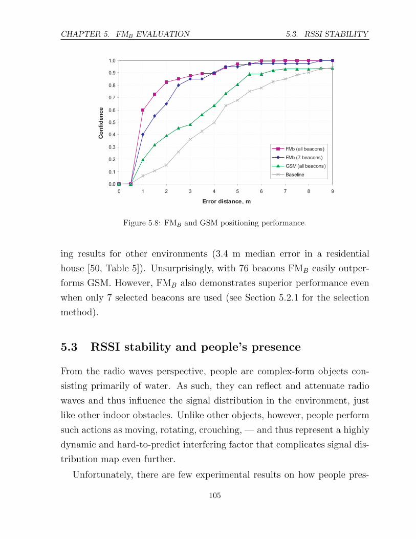
CHAPTER 5. FMB EVALUATION 5.3. RSSI STABILITY
Figure 5.8: FMB and GSM positioning performance.
ing results for other environments (3.4 m median error in a residential
house [50, Table 5]). Unsurprisingly, with 76 beacons FMB easily outper-
forms GSM. However, FMB also demonstrates superior performance even
when only 7 selected beacons are used (see Section 5.2.1 for the selection
method).
5.3 RSSI stability and people’s presence
From the radio waves perspective, people are complex-form objects con-
sisting primarily of water. As such, they can reflect and attenuate radio
waves and thus influence the signal distribution in the environment, just
like other indoor obstacles. Unlike other objects, however, people perform
such actions as moving, rotating, crouching, — and thus represent a highly
dynamic and hard-to-predict interfering factor that complicates signal dis-
tribution map even further.
Unfortunately, there are few experimental results on how people pres-
105

5.3. RSSI STABILITY CHAPTER 5. FMB EVALUATION
ence and movement influence radio-based positioning system performance.
Moreover, the existing results are contradictory. Zemek et al. [35] per-
formed experiments in a shopping center and found that presence of mov-
ing people has little impact on positioning accuracy. In contrast, several
works evaluated Wi-Fi based positioning systems, and found that the posi-
tioning accuracy drops dramatically when the mobile client is surrounded
by people [7, 36].
In order to evaluate the RSSI dependence on people presence, two exper-
iments have been conducted in indoor environments with different crowd
intensity.
5.3.1 Experiment 1 (medium activity levels)
The first experiment took place in a university mensa (canteen). The envi-
ronment was a square-shaped room of about 30×30 meters; the maximum
capacity was 150 people. Two datasets of 50 minutes each have been col-
lected at canteen peak hours (13–14 o’clock) and at the evening (18–19
o’clock) when the room was empty. During the lunch-time phase of the
experiment, the canteen occupation varied from 70% in the beginning to
90% in the peak time and to about 20% near the closing time (Figure 5.9).
Figure 5.9: Canteen occupation profile during the “crowded” phase of the first experiment.
106
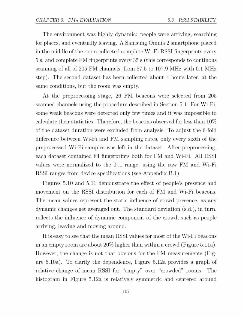
CHAPTER 5. FMB EVALUATION 5.3. RSSI STABILITY
The environment was highly dynamic: people were arriving, searching
for places, and eventually leaving. A Samsung Omnia 2 smartphone placed
in the middle of the room collected complete Wi-Fi RSSI fingerprints every
5 s, and complete FM fingerprints every 35 s (this corresponds to continous
scanning of all of 205 FM channels, from 87.5 to 107.9 MHz with 0.1 MHz
step). The second dataset has been collected about 4 hours later, at the
same conditions, but the room was empty.
At the preprocessing stage, 26 FM beacons were selected from 205
scanned channels using the procedure described in Section 5.1. For Wi-Fi,
some weak beacons were detected only few times and it was impossible to
calculate their statistics. Therefore, the beacons observed for less than 10%
of the dataset duration were excluded from analysis. To adjust the 6-fold
difference between Wi-Fi and FM sampling rates, only every sixth of the
preprocessed Wi-Fi samples was left in the dataset. After preprocessing,
each dataset contained 84 fingerprints both for FM and Wi-Fi. All RSSI
values were normalized to the 0..1 range, using the raw FM and Wi-Fi
RSSI ranges from device specifications (see Appendix B.1).
Figures 5.10 and 5.11 demonstrate the effect of people’s presence and
movement on the RSSI distribution for each of FM and Wi-Fi beacons.
The mean values represent the static influence of crowd presence, as any
dynamic changes get averaged out. The standard deviation (s.d.), in turn,
reflects the influence of dynamic component of the crowd, such as people
arriving, leaving and moving around.
It is easy to see that the mean RSSI values for most of the Wi-Fi beacons
in an empty room are about 20% higher than within a crowd (Figure 5.11a).
However, the change is not that obvious for the FM measurements (Fig-
ure 5.10a). To clarify the dependence, Figure 5.12a provides a graph of
relative change of mean RSSI for “empty” over “crowded” rooms. The
histogram in Figure 5.12a is relatively symmetric and centered around
107

5.3. RSSI STABILITY CHAPTER 5. FMB EVALUATION
(a) Mean FM RSSI
(b) FM RSSI standard deviation
Figure 5.10: FM RSSI statistics for empty and crowded environment.
(a) Mean Wi-Fi RSSI (b) Wi-Fi RSSI standard deviation
Figure 5.11: Wi-Fi RSSI statistics for empty and crowded environment.
108
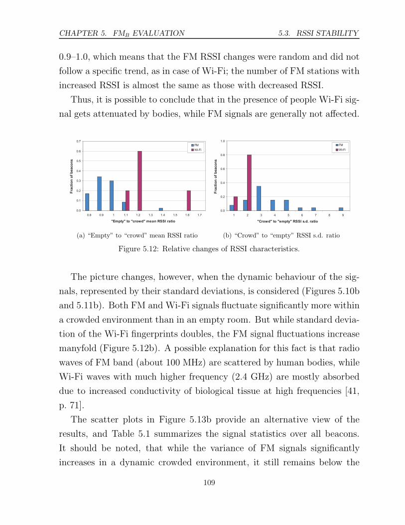
CHAPTER 5. FMB EVALUATION 5.3. RSSI STABILITY
0.9–1.0, which means that the FM RSSI changes were random and did not
follow a specific trend, as in case of Wi-Fi; the number of FM stations with
increased RSSI is almost the same as those with decreased RSSI.
Thus, it is possible to conclude that in the presence of people Wi-Fi sig-
nal gets attenuated by bodies, while FM signals are generally not affected.
(a) “Empty” to “crowd” mean RSSI ratio (b) “Crowd” to “empty” RSSI s.d. ratio
Figure 5.12: Relative changes of RSSI characteristics.
The picture changes, however, when the dynamic behaviour of the sig-
nals, represented by their standard deviations, is considered (Figures 5.10b
and 5.11b). Both FM and Wi-Fi signals fluctuate significantly more within
a crowded environment than in an empty room. But while standard devia-
tion of the Wi-Fi fingerprints doubles, the FM signal fluctuations increase
manyfold (Figure 5.12b). A possible explanation for this fact is that radio
waves of FM band (about 100 MHz) are scattered by human bodies, while
Wi-Fi waves with much higher frequency (2.4 GHz) are mostly absorbed
due to increased conductivity of biological tissue at high frequencies [41,
p. 71].
The scatter plots in Figure 5.13b provide an alternative view of the
results, and Table 5.1 summarizes the signal statistics over all beacons.
It should be noted, that while the variance of FM signals significantly
increases in a dynamic crowded environment, it still remains below the
109

5.3. RSSI STABILITY CHAPTER 5. FMB EVALUATION
(a) Empty (b) Crowded
Figure 5.13: Mean vs. s.d. of FM and Wi-Fi RSSI in the empty and crowded canteen.
Table 5.1: RSSI statistics over all beacons (student canteen).
FM Wi-FiMean SD Mean SD
Empty 0.147 4.60 · 10−3 0.259 1.12 · 10−2
Crowd 0.150 1.43 · 10−2 0.211 1.90 · 10−2
level of Wi-Fi’s fluctuations. Thus, FM fingerprints are more stable than
Wi-Fi ones in less populated environments; in crowded environments both
technologies are prone to similar amount of noise.
5.3.2 Experiment 2 (low activity levels)
The second experiment considered a less dynamic environment and focused
on the distortions of FM and Wi-Fi signals caused by people performing
conventional office activities. Signal characteristics have been compared
for three scenarios: empty room in daytime, populated room in normal
office hours, and empty room in nighttime. The two empty-room scenarios
(daytime and nighttime) have been considered in order to recognize FMB
signal distortions that could be introduced by external noise sources, such
as city traffic and activities in adjacent rooms. Such noises are generally
110

CHAPTER 5. FMB EVALUATION 5.3. RSSI STABILITY
attributed to human activities, which are minimal in the nighttime.
A Samsung Omnia 2 smartphone has been placed on a desk in the middle
of the office (Figure 4.1) and recorded FM and Wi-Fi RSSI fingerprints for
3 full days, Saturday to Monday. From the recorded data, three 6-hour
datasets have been extracted:
1. Sunday, 12 to 18 o’clock (“empty room, daytime”);
2. Monday, 0 to 6 o’clock (“empty room, nighttime”); and
3. Monday, 12 to 18 o’clock (“populated room”).
On Monday, two people were present in the room; the desk with the
smartphone remained unattended for the whole period. The collected FM
fingerprints included 205 channels and repeated every 36 s (this value cor-
responds to the maximum FM scanning speed of the device). Wi-Fi fin-
gerprints were acquired every 6 s.
The preprocessing phase included normalization of raw RSSI values to
the range 0..1, using the minimum and maximum RSSI values reported
in device specification (see Appendix B.1). In order to accommodate for
different sampling rates of FM and Wi-Fi, only every sixth Wi-Fi sample
has been considered. Some weak Wi-Fi beacons were detected only few
times during the experiment. In order to ensure a fair comparison, the
beacons present in less than 10% of fingerprints, were excluded. For the
FM data, the 205-channel fingerprints were narrowed to 23 active stations,
using the approach described in Section 5.1. After preprocessing, each
dataset contained 592 samples with 23 FM and 13 Wi-Fi beacons.
Figures 5.14 present a per-beacon comparison of RSSI statistics for each
scenario. Evidently, both FM and Wi-Fi signal characteristics in an empty
room remained virtually the same, irrespective of time. During the work
hours, however, the situation changes; both wireless modules detect in-
creased fluctuations of the received signals, reflected by significantly higher
111

5.3. RSSI STABILITY CHAPTER 5. FMB EVALUATION
(a) Mean FM RSSI (b) Standard deviation of FM RSSI
(c) Mean Wi-Fi RSSI (d) Standard deviation of Wi-Fi RSSI
Figure 5.14: FM and Wi-Fi RSSI statistics for an office environment.
standard deviation of RSSI values. Although the increase is larger for the
FM, the FM RSSI deviation still remains well below that of Wi-Fi, partly
due to weaker signals. Remarkably, mean FM RSSI was not affected by
people’s presence. Average Wi-Fi readings, however, slightly decreased.
An integral view of mean values and their deviations is presented in Fig-
ure 5.15.
The results presented in Table 5.2 are in a good agreement with the
previous experiment (Section 5.3.1). Mean FMB RSSI values are indiffer-
ent to the presence of people, while Wi-Fi values slightly decrease. Both
technologies demonstrate stronger fluctuations of signals in populated envi-
ronments; moreover, the mean Wi-Fi RSS slightly decreases. This behavior
112
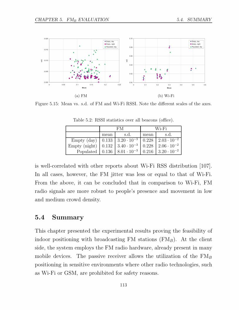
CHAPTER 5. FMB EVALUATION 5.4. SUMMARY
(a) FM (b) Wi-Fi
Figure 5.15: Mean vs. s.d. of FM and Wi-Fi RSSI. Note the different scales of the axes.
Table 5.2: RSSI statistics over all beacons (office).
FM Wi-Fimean s.d. mean s.d.
Empty (day) 0.133 3.20 · 10−3 0.228 2.03 · 10−2
Empty (night) 0.132 3.40 · 10−3 0.228 2.06 · 10−2
Populated 0.136 8.01 · 10−3 0.216 3.20 · 10−2
is well-correlated with other reports about Wi-Fi RSS distribution [107].
In all cases, however, the FM jitter was less or equal to that of Wi-Fi.
From the above, it can be concluded that in comparison to Wi-Fi, FM
radio signals are more robust to people’s presence and movement in low
and medium crowd density.
5.4 Summary
This chapter presented the experimental results proving the feasibility of
indoor positioning with broadcasting FM stations (FMB). At the client
side, the system employs the FM radio hardware, already present in many
mobile devices. The passive receiver allows the utilization of the FMB
positioning in sensitive environments where other radio technologies, such
as Wi-Fi or GSM, are prohibited for safety reasons.
113

5.4. SUMMARY CHAPTER 5. FMB EVALUATION
Table 5.3: Summary of FMB, Wi-Fi and GSM indoor positioning accuracy.
Confidence FMB Wi-Fi GSM FMB (10% of beacons)
50% 0.9 1.6 3.1 1.367% 1.3 1.9 4.2 2.190% 3.4 3.5 6.2 4.095% 4.7 4.0 9.1 4.9
The summary of FMB, Wi-Fi and GSM positioning accuracy measured
in same environment is presented in Table 5.3. In comparison to Wi-Fi,
FMB provides superior accuracy at confidence levels of up to 90% in same-
environment tests. Using only 10% of stations, FMB performed similar to
Wi-Fi. In contrast to Wi-Fi systems, however, the FMB localization does
not require any in-building infrastructure and consequently has minimal
hardware costs. The GSM, which also uses external beacons, demonstrated
far inferior accuracy than either FMB or Wi-Fi.
This chapter also evaluated how the presence of small and medium num-
bers of people influences FM and Wi-Fi signal strengths. It has been found
that the average Wi-Fi RSSI consistently decreased in the presence of peo-
ple: by 20% in student canteen at peak hours and by 5% in a typical
office with few people. For FM, the mean RSSI changed differently across
stations; for most (80%) of the stations the shift was within 10%. The
standard deviation of the signal strengths for both technologies signifi-
cantly increased in populated environments: by 50–70% for Wi-Fi and by
135–170% for FM. Despite the higher increase, the standard deviation of
FM RSS was in all cases lower or equal to that of Wi-Fi.
114

Chapter 6
Application scenario
The FM positioning system described in previous chapters has been suc-
cessfully used within a research project which studied variations of psycho-
logical state in office workers [123, 124].
The hypothesis of the project was that people who spend most time
sitting at their desks would have worse mood at the end of the day than
those who make regular pauses, such as coffee breaks or socialization with
colleagues. Another hypothesis was that some working activities may have
higher impact and induce more negative mood than others (for example,
missed lunch or repetitive meetings with a boss).
In this respect, the potential working activities and socialization events
were associated with the locations where they typically occur: office (work-
ing), conference room (being at a meeting), coffee room or balcony (having
a break), canteen or cafeteria (having lunch). Apart from the location, a
number of psychophysiological parameters were recorded to monitor the
mood state. The parameters were identified from clinical studies and in-
cluded body movements level, heart rate and its variability, sleep quality
and a number of mood characteristics. The monitoring platform consisted
of a Samsung Omnia 2 smartphone running MyExperience tool [115] cus-
tomized for the project, and an external Bluetooth-connected sensor from
115
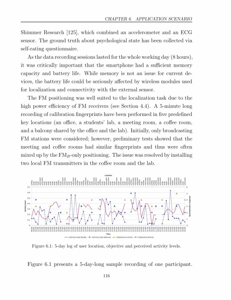
CHAPTER 6. APPLICATION SCENARIO
Shimmer Research [125], which combined an accelerometer and an ECG
sensor. The ground truth about psychological state has been collected via
self-rating questionnaire.
As the data recording sessions lasted for the whole working day (8 hours),
it was critically important that the smartphone had a sufficient memory
capacity and battery life. While memory is not an issue for current de-
vices, the battery life could be seriously affected by wireless modules used
for localization and connectivity with the external sensor.
The FM positioning was well suited to the localization task due to the
high power efficiency of FM receivers (see Section 4.4). A 5-minute long
recording of calibration fingerprints have been performed in five predefined
key locations (an office, a students’ lab, a meeting room, a coffee room,
and a balcony shared by the office and the lab). Initially, only broadcasting
FM stations were considered; however, preliminary tests showed that the
meeting and coffee rooms had similar fingerprints and thus were often
mixed up by the FMB-only positioning. The issue was resolved by installing
two local FM transmitters in the coffee room and the lab.
Figure 6.1: 5-day log of user location, objective and perceived activity levels.
Figure 6.1 presents a 5-day-long sample recording of one participant.
116
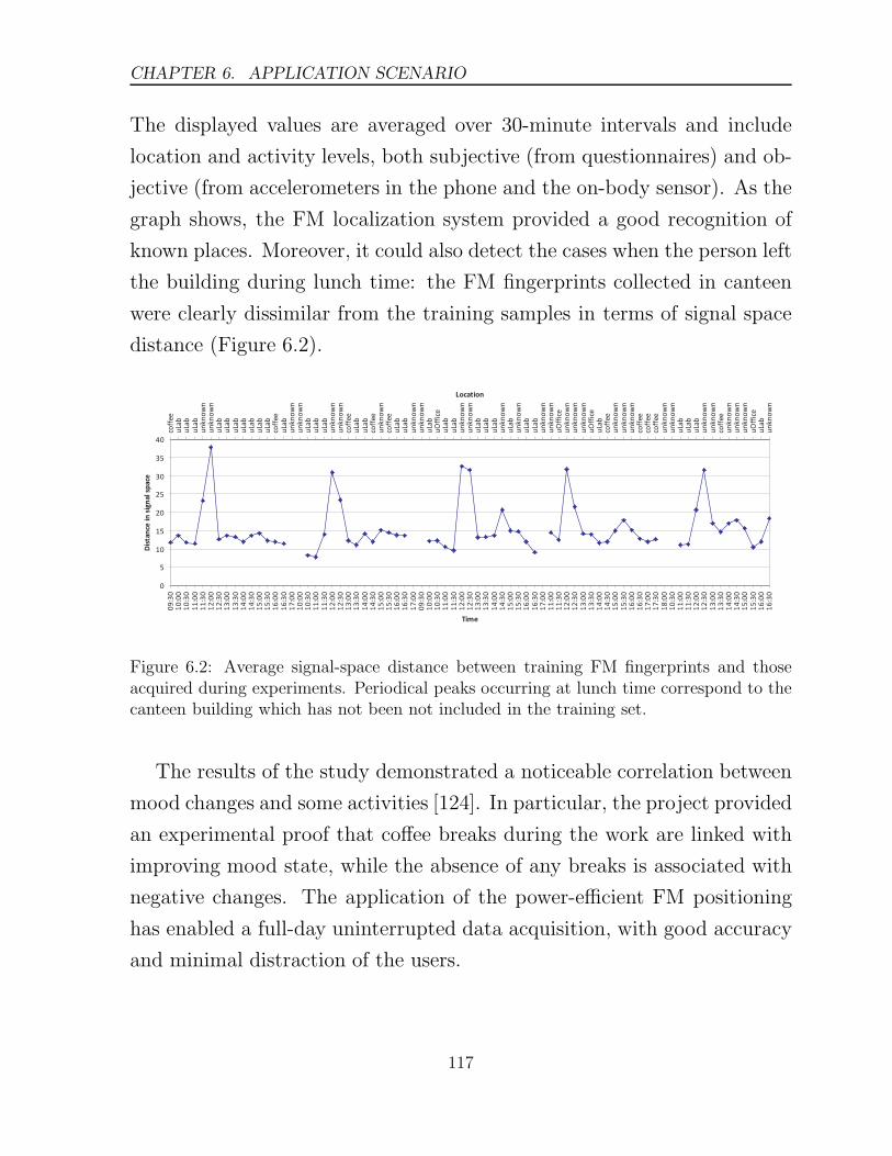
CHAPTER 6. APPLICATION SCENARIO
The displayed values are averaged over 30-minute intervals and include
location and activity levels, both subjective (from questionnaires) and ob-
jective (from accelerometers in the phone and the on-body sensor). As the
graph shows, the FM localization system provided a good recognition of
known places. Moreover, it could also detect the cases when the person left
the building during lunch time: the FM fingerprints collected in canteen
were clearly dissimilar from the training samples in terms of signal space
distance (Figure 6.2).
Figure 6.2: Average signal-space distance between training FM fingerprints and thoseacquired during experiments. Periodical peaks occurring at lunch time correspond to thecanteen building which has not been not included in the training set.
The results of the study demonstrated a noticeable correlation between
mood changes and some activities [124]. In particular, the project provided
an experimental proof that coffee breaks during the work are linked with
improving mood state, while the absence of any breaks is associated with
negative changes. The application of the power-efficient FM positioning
has enabled a full-day uninterrupted data acquisition, with good accuracy
and minimal distraction of the users.
117

Chapter 7
Conclusion
The current de-facto standard of indoor positioning, Wi-Fi based local-
ization, has a number of constraints, such as limited coverage and low
battery life. The solution proposed in this thesis leverages FM radio sig-
nals for indoor positioning; the system was proven to provide an accuracy
comparable to Wi-Fi, with significantly higher coverage and battery life.
Two types of signal sources have been considered: local FM transmitters
and broadcasting FM stations.
The first approach, FML, employed local short-range FM transmitters,
the consumer-grade devices which do not require licensing. FML localiza-
tion demonstrated the performance similar to Wi-Fi (see Figure 7.1 below).
A combination of FML and Wi-Fi provided a better positioning accuracy
than either of the systems used alone.
The second approach leveraged radio signals from broadcasting FM sta-
tions (FMB). FMB localization does not require any in-building infras-
tructure and thus has zero hardware costs. Moreover, the coverage of FM
broadcasts is much wider than that of Wi-Fi or cellular networks. Finally,
due to the high number of available stations, in the laboratory tests the
FMB system provided better accuracy than Wi-Fi in 90% of the cases
(Figure 7.1). The performance of GSM positioning, which also employs
119
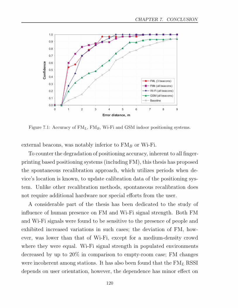
CHAPTER 7. CONCLUSION
Figure 7.1: Accuracy of FML, FMB, Wi-Fi and GSM indoor positioning systems.
external beacons, was notably inferior to FMB or Wi-Fi.
To counter the degradation of positioning accuracy, inherent to all finger-
printing based positioning systems (including FM), this thesis has proposed
the spontaneous recalibration approach, which utilizes periods when de-
vice’s location is known, to update calibration data of the positioning sys-
tem. Unlike other recalibration methods, spontaneous recalibration does
not require additional hardware nor special efforts from the user.
A considerable part of the thesis has been dedicated to the study of
influence of human presence on FM and Wi-Fi signal strength. Both FM
and Wi-Fi signals were found to be sensitive to the presence of people and
exhibited increased variations in such cases; the deviation of FM, how-
ever, was lower than that of Wi-Fi, except for a medium-density crowd
where they were equal. Wi-Fi signal strength in populated environments
decreased by up to 20% in comparison to empty-room case; FM changes
were incoherent among stations. It has also been found that the FML RSSI
depends on user orientation, however, the dependence has minor effect on
120

CHAPTER 7. CONCLUSION
positioning accuracy and cannot be utilized to recognize user direction from
signal fingerprints.
The main contributions of this thesis are:
• demonstration of feasibility of accurate indoor localization using lo-
cal short-range FM transmitters, with accuracy comparable to Wi-Fi
based systems;
• demonstration of feasibility of accurate indoor positioning using sig-
nals of broadcasting FM stations, with accuracy superior to Wi-Fi
and GSM based systems (for confidence of up to 90% and in all cases,
respectively);
• an analysis and quantitative evaluation of the influence of human pres-
ence on the stability of FM and Wi-Fi signal strengths;
• a method for countering the accuracy degradation of fingerprinting-
based positioning systems.
The main advantage of the presented concepts is that they can be readily
deployed: FM receivers are available in many mobile devices. In compar-
ison to Wi-Fi, FM tuner has lower power consumption and as a result
provides 2.6 to 5.5 times longer battery life in localization mode. The
client-side FM radio is a passive receiver — thus, FM positioning may be
used in sensitive areas where radio transmission, such as Wi-Fi or GSM,
is prohibited for safety or security reasons. At the moment, FMB is the
only wireless indoor positioning technology capable to work in a completely
passive manner, without introducing any additional signals into the envi-
ronment. Other systems either require an infrastructure of transmitting
beacons (Wi-Fi, FML, Bluetooth, RFID, UWB, ultrasound, infrared) or
employ a transmitting mobile device (cellular networks).
121

7.1. FUTURE WORK CHAPTER 7. CONCLUSION
7.1 Future work
The FM positioning tests in this thesis comprised two separate phases: fin-
gerprints collection for the whole environment, followed by their analysis.
However, in real life people move along trajectories, so that the next lo-
cation depends on the previous one. Taking into account this information
could significantly improve the confidence of position estimates.
Another concern regarding real-time FM localization is the time re-
quired to collect a wide FM fingerprint. Scanning several dozens of FM
channels may take a considerable time; in the meanwhile, the location can
change. Constraining the scans to only a subset of channels would impact
the accuracy. A smart channel selection algorithm could be a more appro-
priate solution. Due to the heterogeneity of indoor environments, different
points require different number of beacons for localization. From the cal-
ibration data, the mobile device can calculate a policy which specifies the
beacon to be scanned next in order to minimize the ambiguity of location
estimation. Thus, the beacons can be scanned in the optimal order, de-
pending on the already acquired data. This will result in faster convergence
of location estimates and, consequently, fast yet accurate localization.
At the moment, it is unclear if or how often the broadcasting FM sta-
tions change their transmission site, so that the signal starts to arrive from
a different direction. Such changes would obviously affect the positioning
performance. It might be possible to detect such cases by clustering the
channels which fluctuate in a correlated manner as the client moves — this
would mean that these stations are broadcasted from the same site. A
station which changed its location would stand out from the correlation.
Finally, while FM radio waves are theoretically insensitive to atmo-
spheric conditions, the influence of outdoor factors (such as weather, vehi-
cles) on the FMB performance requires further experimental evaluation.
122
Bibliography
[1] A. Youssef, J. Krumm, E. Miller, G. Cermak, and E. Horvitz. Com-
puting location from ambient FM radio signals. In IEEE Wireless
Communications and Networking Conference (WCNC’05), volume 2,
pages 824–829, March 2005.
[2] Shih-Hau Fang, Jen-Chian Chen, Hao-Ru Huang, and Tsung-Nan
Lin. Is FM a RF-based positioning solution in a metropolitan-scale
environment? A probabilistic approach with radio measurements
analysis. IEEE Transactions on Broadcasting, 55(3):577–588, Sept.
2009. ISSN 0018-9316.
[3] Homayoun Hashemi. The indoor radio propagation channel. Pro-
ceedings of the IEEE, 81(7):943–968, 1993.
[4] Department of Defense World Geodetic System 1984: Its defini-
tion and relationships with local geodetic systems. Technical Re-
port TR8350.2, National Imagery and Mapping Agency, 1997. On-
line: http://earth-info.nga.mil/GandG/publications/tr8350.
2/wgs84fin.pdf, retrieved 2011-03-12.
[5] Nathaniel Bowditch. The American Practical Navigator, chapter
Dead reckoning, pages 113–118. National Imagery and Mapping
Agency, USA, 1995.
123

BIBLIOGRAPHY
[6] International Telecommunication Union. Recommendation ITU-R
P.1238: Propagation data and prediction methods for the planning
of indoor radiocommunication systems and radio local area networks
in the frequency range 900 MHz to 100 GHz, 2009. Retrieved 2011-
01-18.
[7] Y.C. Chen, J.R. Chiang, H. Chu, P. Huang, and A.W. Tsui. Sensor-
assisted Wi-Fi indoor location system for adapting to environmental
dynamics. In Proceedings of the 8th ACM international symposium
on Modeling, analysis and simulation of wireless and mobile systems,
pages 118–125. ACM, 2005. ISBN 1595931880.
[8] N. Bulusu, J. Heidemann, and D. Estrin. GPS-less low-cost outdoor
localization for very small devices. Personal Communications, IEEE,
7(5):28–34, 2000.
[9] Emiliano Trevisani and Andrea Vitaletti. Cell-ID location technique,
limits and benefits: an experimental study. In Proceedings of the
6th IEEE Workshop on Mobile Computing Systems and Applications
(WMCSA 2004), pages 51–60, Washington, DC, USA, 2004. IEEE
Computer Society. ISBN 0-7695-2258-0.
[10] Jurgen Bohn. iPOS: A fault-tolerant and adaptive multi-sensor po-
sitioning architecture with QoS guarantees. Sensor Review, 27(3):
239–249, 2007.
[11] L. Liao, D. Fox, J. Hightower, H. Kautz, and D. Schulz. Voronoi
Tracking: Location Estimation Using Sparse and Noisy Sensor Data.
In Proceedings of the IEEE/RSJ International Conference on Intel-
ligent Robots and Systems (IROS’03), 2003.
[12] Cristiano di Flora, Massimo Ficco, and Stefano Russo. Indoor Po-
sitioning for Location-Aware Applications on Java-Based Mobile De-
124

BIBLIOGRAPHY
vices, volume 3292 of Lecture Notes in Computer Science, chapter On
the Move to Meaningful Internet Systems 2004: OTM 2004 Work-
shops, pages 383–393. Springer Berlin / Heidelberg, 2004.
[13] US Department of Defence. GPS SPS Performance Stan-
dard. Online: http://www.navcen.uscg.gov/gps/geninfo/
2008SPSPerformanceStandardFINAL.pdf, September 2008.
[14] Les W. Barclay, editor. Propagation of Radiowaves. The Institution
of Engineering and Technology, second edition, 2002.
[15] International Telecommunication Union. Recommendation ITU-R
P.1546: Method for point-to-area predictions for terrestrial services
in the frequency range 30 MHz to 3 000 MHz, 2009.
[16] International Telecommunication Union. Recommendation ITU-
R P.840-4: Attenuation due to clouds and fog. Online: http:
//www.itu.int/rec/R-REC-P.840-4-200910-I/en, October 2009.
Retrieved 2011-01-18.
[17] International Telecommunication Union. Recommendation ITU-R
P.833-6: Attenuation in vegetation. Online: http://www.itu.int/
rec/R-REC-P.833-6-200702-I/en, February 2007. Retrieved 2011-
01-18.
[18] D. Molkdar. Review on radio propagation into and within buildings.
In IEE Proceedings-H (Microwaves, Antennas and Propagation), vol-
ume 138, pages 61–73. IET, 1991.
[19] M. Ocana, L.M. Bergasa, M.A. Sotelo, J. Nuevo, and R. Flores. In-
door robot localization system using WiFi signal measure and min-
imizing calibration effort. In Proceedings of the IEEE International
125
BIBLIOGRAPHY
Symposium on Industrial Electronics (ISIE 2005), volume 4, pages
1545–1550. IEEE, 2005. ISBN 0780387384.
[20] P. Bahl and V. N. Padmanabhan. RADAR: An in-building RF-based
user location and tracking system. In Proceedings of 9th Annual Joint
Conference of the IEEE Computer and Communications Societies
(INFOCOM 2000), volume 2, pages 775–784, 26-30 March 2000.
[21] F. Seco, A. R. Jimenez, C. Prieto, J. Roa, and K. Koutsou. A survey
of mathematical methods for indoor localization. In Proc. IEEE Int.
Symp. Intelligent Signal Processing WISP 2009, pages 9–14, 2009.
[22] Tsung-Nan Lin and Po-Chiang Lin. Performance comparison of in-
door positioning techniques based on location fingerprinting in wire-
less networks. In Proceedings of International Conference on Wireless
Networks, Communications and Mobile Computing, volume 2, pages
1569–1574, 2005.
[23] R. Battiti, N.T. Le, and A. Villani. Location-aware computing: a
neural network model for determining location in wireless LANs.
Technical report, University of Trento, 2002.
[24] T. Roos, P. Myllymaki, H. Tirri, P. Misikangas, and J. Sievanen. A
probabilistic approach to WLAN user location estimation. Interna-
tional Journal of Wireless Information Networks, 9(3):155–164, 2002.
[25] M. Chen, T. Sohn, D. Chmelev, D. Haehnel, J. Hightower, J. Hughes,
A. LaMarca, F. Potter, I. Smith, and A. Varshavsky. Practical
metropolitan-scale positioning for GSM phones. In Paul Dourish
and Adrian Friday, editors, Proceedings of the 8th International Con-
ference on Ubiquitous Computing (UbiComp 2006), volume 4206 of
Lecture Notes in Computer Science, pages 225–242, Orange County,
CA, USA, September 17–21 2006. Springer Berlin / Heidelberg.
126

BIBLIOGRAPHY
[26] B. Ferris, D. Haehnel, and D. Fox. Gaussian processes for signal
strength-based location estimation. In Proc. of Robotics: Science
and Systems, 2006.
[27] A. Schwaighofer, M. Grigoras, V. Tresp, and C. Hoffmann. GPPS: A
Gaussian process positioning system for cellular networks. In Proceed-
ings of the 17th Annual Conference on Neural Information Processing
Systems (NIPS-2003), volume 16, 2004.
[28] T. Mitchell. Machine Learning. ISBN 0070428077. McGraw Hill,
1997.
[29] V. Seshadri, G.V. Zaruba, and M. Huber. A bayesian sampling ap-
proach to in-door localization of wireless devices using received signal
strength indication. In Pervasive Computing and Communications,
2005. PerCom 2005. Third IEEE International Conference on, Vol.,
Iss., pages 75–84, 8-12 March 2005.
[30] M. Brunato and R. Battiti. Statistical learning theory for location
fingerprinting in wireless LANs. Computer Networks, 47(6):825–845,
2005.
[31] Nicola Segata and Enrico Blanzieri. Fast and scalable local kernel
machines. The Journal of Machine Learning Research, 11:1883–1926,
2010. ISSN 1532-4435.
[32] X. Chai and Q. Yang. Reducing the calibration effort for location
estimation using unlabeled samples. pages 95–104. IEEE Computer
Society, 2005.
[33] J. Krumm and J. Platt. Minimizing calibration effort for an in-
door 802.11 device location measurement system. Technical Report
127
BIBLIOGRAPHY
MSR-TR-2003-82, Microsoft Research, Microsoft Corporation, One
Microsoft Way, Redmond, WA 98052, November 13 2003.
[34] A. LaMarca, J. Hightower, I. Smith, and S. Consolvo. Self-mapping
in 802.11 location systems. In Beigl et al. [129], pages 87–104.
[35] Radim Zemek, Masahiro Takashima, Dapeng Zhao, Shinsuke Hara,
Kentaro Yanagihara, Kiyoshi Fukui, Shigeru Fukunaga, and Ken-
ichi Kitayama. Effect of walking people on target location estimation
performance in an IEEE 802.15.4 wireless sensor network. IEICE
Transactions on Communications, 90(10):2809–2816, 2007.
[36] L. Chan, J. Chiang, Y. Chen, C. Ke, J. Hsu, and H. Chu. Collabo-
rative localization: Enhancing WiFi-based position estimation with
neighborhood links in clusters. In Proceedings of the 4th Conference
on Pervasive Computing (Pervasive 2006). Springer, 2006.
[37] L.F.M. de Moraes and B.A.A. Nunes. Calibration-free WLAN loca-
tion system based on dynamic mapping of signal strength. In Proceed-
ings of the 4th ACM international workshop on Mobility management
and wireless access, pages 92–99. ACM New York, NY, USA, 2006.
[38] P. Bahl, V.N. Padmanabhan, and A. Balachandran. Enhancements
to the RADAR user location and tracking system. Technical Report
MSR-TR-2000-12, Microsoft Research, Redmond, WA, USA, 2000.
[39] M. A. Youssef, A. Agrawala, and A. U. Shankar. WLAN location
determination via clustering and probability distributions. In Pro-
ceedings of the 1st IEEE International Conference on Pervasive Com-
puting and Communications (PerCom), pages 143–150, 2003.
128

BIBLIOGRAPHY
[40] T. Roos, P. Myllymaki, and H. Tirri. A statistical modeling approach
to location estimation. IEEE Transactions on Mobile Computing, 1
(1):59–69, 2002.
[41] Carl H. Durney, Habib Massoudi, and Magdy F. lskander. Ra-
diofrequency radioation dosimetry handbook. Technical Report
USAFSAM-TR-85-73, The University of Utah, 1986.
[42] Sebastian Gansemer and Uwe Großmann. RSSI-based Euclidean Dis-
tance algorithm for indoor positioning adapted for the use in dynam-
ically changing WLAN environments and multi-level buildings. 2010.
[43] A. LaMarca, Y. Chawathe, S. Consolvo, J. Hightower, I. Smith,
J. Scott, T. Sohn, J. Howard, J. Hughes, F. Potter, J. Tabert, P. Pow-
eldge, G. Borriello, and B. Schilit. Place Lab: Device positioning
using radio beacons in the wild. In Hans W. Gellersen, Roy Want,
and Albrecht Schmidt, editors, Proceedings of the 3rd International
Conference on Pervasive Computing (Pervasive 2005), volume 3468
of Lecture Notes in Computer Science, pages 116–133, Munich, Ger-
many, May 8–13 2005. Springer.
[44] Gunter Lorenz and Peer-Axel Kroeske. Radio frequencies & trans-
mitter maps worldwide. Online: http://fmscan.org. Retrieved
2011-01-17.
[45] Ryan Winfield Woodings and Mark Gerrior. Avoiding in-
terference in the 2.4 GHz ISM band. Online: http:
//www.eetimes.com/design/microwave-rf-design/4012556/
Avoiding-Interference-in-the-2-4-GHz-ISM-Band, February
2005. Retrieved 2010-01-28.
[46] Ad Kamerman and Nedim Erkocevic. Microwave oven interference
on wireless LANs operating in the 2.4 GHz ISM band. In The 8th
129

BIBLIOGRAPHY
IEEE International Symposium on Personal, Indoor and Mobile Ra-
dio Communications (PIMRC ’97), volume 3, pages 1221–1227, 1997.
[47] Manish Anand, Edmund B. Nightingale, and Jason Flinn. Self-tuning
wireless network power management. Wireless Networks, 11:451–469,
July 2005. ISSN 1022-0038.
[48] H. Laitinen, J. Lahteenmaki, and T. Nordstrom. Database correlation
method for GSM location. In Proceedings of the 53rd IEEE Vehicu-
lar Technology Conference (VTC 2001), volume 4, pages 2504–2508,
2001.
[49] C. Drane, M. Macnaughtan, and C. Scott. Positioning GSM tele-
phones. Communications Magazine, IEEE, 36(4):46–54, 1998.
[50] V. Otsason, A. Varshavsky, A. LaMarca, and E. de Lara. Accurate
GSM indoor localization. In Beigl et al. [129], pages 141–158.
[51] Waqas ur Rehman, Eyal de Lara, and Stefan Saroiu. CILoS: a CDMA
indoor localization system. In Proceedings of the 10th international
conference on Ubiquitous computing (UbiComp 2008) ubi [130], pages
104–113. ISBN 978-1-60558-136-1.
[52] Andrew Rice and Simon Hay. Decomposing power measurements for
mobile devices. per [128].
[53] International Telecommunication Union. Recommendation ITU-R
P.620: Propagation data required for the evaluation of coordination
distances in the frequency range 100 MHz to 105 GHz, March 2005.
Retrieved 2011-01-18.
[54] J. Krumm, G. Cermak, and E. Horvitz. RightSPOT: A novel sense
of location for a smart personal object. In Anind K. Dey, Albrecht
Schmidt, and Joseph F. McCarthy, editors, Proceedings of the 5th
130

BIBLIOGRAPHY
International Conference on Ubiquitous Computing (Ubicomp 2003),
volume 2864 of Lecture Notes in Computer Science, pages 36–43,
Seattle, WA, USA, October 12-15 2003. Springer Berlin / Heidelberg.
[55] S.H. Fang and T.N. Lin. Cooperative multi-radio localization in het-
erogeneous wireless networks. IEEE Transactions on Wireless Com-
munications, 9(5):1547–1551, 2010. ISSN 1536-1276.
[56] International Telecommunication Union. Recommendation ITU-R
P.1812: A path-specific propagation prediction method for point-to-
area terrestrial services in the VHF and UHF bands, 2009.
[57] A. Giordano, D. Borkowski, and D. Kelley. Location enhanced cellu-
lar information services. In Proceedings of the 5th IEEE International
Symposium on Personal, Indoor and Mobile Radio Communications,
volume 4, pages 1143–1145, 1994.
[58] David C. Kelley, David T. Rackley, and Victor P. Berglund. Naviga-
tion and positioning system and method using uncoordinated beacon
signals. US Patent No. 5173710, 1992.
[59] David C. Kelley, David T. Rackley, and Victor P. Berglund. Naviga-
tion and positioning system and method using uncoordinated beacon
signals. US Patent No. 5280295, 1994.
[60] David C. Kelley, Joseph Cisneros, and Louis A. Greenbaum. Naviga-
tion and positioning system and method using uncoordinated becon.
US Patent 5689270, November 1997.
[61] A.G. Bose and W.R. Short. A theoretical and experimental study of
noise and distortion in the reception of FM signals. IEEE Transac-
tions on Broadcasting, 47(2):164–179, June 2001. ISSN 0018-9316.
131

BIBLIOGRAPHY
[62] David A. Howe. Precise frequency dissemination using the 19-kHz
pilot tone on stereo FM radio stations. IEEE Transactions on Broad-
casting, BC-20(1):17–20, March 1974. ISSN 0018-9316.
[63] Federal Communications Commission. Docket no.13506 (FM stereo
final report and order). Technical Report FCC 61-524, Federal Com-
munications Commission, 1961. Retrieved 2010/12/05.
[64] H.D. Griffiths and C.J. Baker. Passive coherent location radar sys-
tems. Part 1: Performance prediction. IEE Proceedings on Radar,
Sonar and Navigation, 152(3):153–159, June 2005. ISSN 1350-2395.
[65] C.J. Baker, H.D. Griffiths, and I. Papoutsis. Passive coherent location
radar systems. Part 2: Waveform properties. IEE Proceedings on
Radar, Sonar and Navigation, 152(3):160–168, June 2005. ISSN 1350-
2395.
[66] A.S. Tasdelen and H. Koymen. Range resolution improvement in
passive coherent location radar systems using multiple FM radio
channels. In The Institution of Engineering and Technology Forum
on Waveform Diversity and Design in Communications, Radar and
Sonar, pages 23 –31, November 2006.
[67] AKM Hossain and W.S. Soh. A comprehensive study of Blue-
tooth signal parameters for localization. In Proceedings of the 18th
IEEE International Symposium on Personal, Indoor and Mobile Ra-
dio Communications (PIMRC 2007), pages 1–5. IEEE, 2007.
[68] J. Hallberg, M. Nilsson, and K. Synnes. Positioning with Bluetooth.
In Proceedings of 10th International Conference on Telecommunica-
tions (ICT 2003), volume 2, pages 954–958, 23 February–1 March
2003.
132
BIBLIOGRAPHY
[69] Ubisense: Precise real-time location. Online: http://www.
ubisense.net, 2010. Retrieved 2011-02-15.
[70] T. Stiefmeier, D. Roggen, G. Ogris, P. Lukowicz, and G. Tr
”oster. Wearable activity tracking in car manufacturing. IEEE Per-
vasive Computing, pages 42–50, 2008. ISSN 1536-1268.
[71] S. N. Patel, K. N. Truong, and G. D. Abowd. PowerLine Positioning:
A practical sub-room-level indoor location system for domestic use.
In Paul Dourish and Adrian Friday, editors, Proceedings of the 8th
International Conference on Ubiquitous Computing (UbiComp 2006),
volume 4206 of Lecture Notes in Computer Science, pages 441–458.
Springer, September 17–21 2006.
[72] E. P. Stuntebeck, S. N. Patel, T. Robertson, M. S. Reynolds, and
G. D. Abowd. Wideband PowerLine Positioning for Indoor Localiza-
tion. In Proceedings of Ubicomp 2008 ubi [130], pages 94–103.
[73] M. Kranz, C. Fischer, and A. Schmidt. A comparative study of
DECT and WLAN signals for indoor localization. In Proceedings
of the IEEE International Conference on Pervasive Computing and
Communications (PerCom 2010) per [128], pages 235–243.
[74] Paolo Vecchia, Rudiger Matthes, Gunde Ziegelberger, James Lin,
Richard Saunders, and Anthony Swerdlow. Exposure to high fre-
quency electromagnetic fields, biological effects and health conse-
quences (100 kHz–300 GHz). Technical Report ICNIRP 16/2009, In-
ternational Commission on Non-Ionizing Radiation Protection, 2009.
URL http://www.icnirp.de/documents/RFReview.pdf. ISBN
978-3-934994-10-2.
[75] Andreas Krause, Asim Smailagic, and Daniel P. Siewiorek. Context-
Aware Mobile Computing: Learning Context-Dependent Personal
133
BIBLIOGRAPHY
Preferences from a Wearable Sensor Array. IEEE Transactions on
Mobile Computing, 5(2):113–127, 2006. ISSN 1536-1233.
[76] M. Methfessel, F.-M. Krause, and K. Tittelbach-Helmrich.
WINDECT STP: Research report on power consumption. Techni-
cal report, ETH Zurich, 2005.
[77] Silicon Laboratories, Inc. Si4702/03 datasheet (Broadcast FM radio
tuner for portable applications), 2008.
[78] V. Pillai, H. Heinrich, D. Dieska, P.V. Nikitin, R. Martinez, and
K.V.S. Rao. An ultra-low-power long range battery/passive RFID
tag for UHF and microwave bands with a current consumption of
700 nA at 1.5 V. IEEE Transactions on Circuits and Systems I:
Regular Papers, 54(7):1500–1512, 2007. ISSN 1549-8328.
[79] Y. Medynskiy, S. Gov, A. Mazalek, and D. Minnen. Wearable RFID
for play. In Proceedings of the Intelligent User Interfaces Tangible
Play Workshop, 2007.
[80] Radio Spectrum Policy Group. The future of radio broadcasting in
Europe: Identified needs, opportunities and possible ways forward.
Technical Report RSPG10-349, European Commission, 2010. URL
http://rspg.groups.eu.int/consultations/consultation_
futradio/rspg10_349_report_future_radio_broadcasting.pdf.
[81] International Telecommunication Union. Recommendation ITU-R
BS.450-3: Transmission standards for FM sound broadcasting at
VHF, 2001.
[82] British Broadcasting Company. England FM transmitters. On-
line: http://www.bbc.co.uk/reception/transmitters/radio/
england_fm.shtml, 2011. Retrieved 2011-01-15.
134

BIBLIOGRAPHY
[83] International Telecommunication Union. Recommendation ITU-
R P.838-3: Specific attenuation model for rain for use in pre-
diction methods. Online: http://www.itu.int/rec/R-REC-P.
838-3-200503-I/en, March 2005. Retrieved 2011-01-18.
[84] K. Leentvaar and J. H. Flint. The capture effect in FM receivers.
IEEE Transactions on Communications, 24:531–539, May 1976.
[85] Jean-Paul Linnartz. Analog Transmission over Fading Channels.
Online: http://www.wirelesscommunication.nl/reference/
chaptr05/analog/analog.htm. Retrieved 2010.12.05.
[86] Adrian J. De Vries. Stereo FM transmission system. US Patent
3133993, May 1964.
[87] International Electrotechnical Commission. IEC 62106 edition 2.
Specification of the radio data system (RDS) for VHF/FM sound
broadcasting in the frequency range from 87,5 to 108,0 MHz, 2009.
[88] International Telecommunication Union. Report BS.2104: FM mod-
ulator interference to broadcast services. Online: http://www.itu.
int/publ/R-REP-BS.2104/en, 2007. Retrieved 2010-01-17.
[89] European Comission. Commission decision 2009/381/EC of 13 may
2009 amending Decision 2006/771/EC on harmonisation of the radio
spectrum for use by short-range devices. Official Jounal of Europoean
Union, 52(L119):32–39, 14 May 2009.
[90] Federal Communications Commission. FCC regulations, part 15.
Retrieved 2009.09.20 from http://www.fcc.gov/oet/info/rules/
part15/PART15_07-10-08.pdf, 10 July 2008.
[91] Hui Liu, H. Darabi, P. Banerjee, and Jing Liu. Survey of wireless
indoor positioning techniques and systems. IEEE Transactions on
135

BIBLIOGRAPHY
Systems, Man, and Cybernetics, Part C: Applications and Reviews,
37(6):1067–1080, 2007. doi: 10.1109/TSMCC.2007.905750.
[92] MP3 player with an embedded FM transmitter. http://www.
koniggaming.com/mp3withfmtransmitter.html[5]icnirp2009-16.
(As accessed on 2009.02.19).
[93] John R. Barry, Edward A. Lee, and David G. Messerschmitt. Digital
Communication. Springer, third edition, 2003. ISBN 978-0792375487.
[94] TDA7088 (FM receiver circuit for battery supply) datasheet, 1996.
[95] Federal Communications Commission. Code of Federal Regula-
tions, part 47, section 73.310: FM technical definitions. Online:
http://www.fcc.gov/mb/audio/bickel/amfmrule.html, 2009. Re-
trieved 2010/12/05.
[96] Federal Communications Commission. Code of Federal Regulations,
part 47, section 73.297: FM stereophonic sound broadcasting. Online:
http://www.fcc.gov/mb/audio/bickel/amfmrule.html, 2009. Re-
trieved 2010/12/05.
[97] Jr. Camp, William O. Method and apparatus for locating a mobile
unit. US Patent 6035202, March 2000.
[98] E. Jacobsen and R. Lyons. The sliding DFT. IEEE Signal Processing
Magazine, 20(2):74–80, 2003. ISSN 1053-5888.
[99] RDS Forum. RDS technical specification: Methods of measure-
ments for RDS receiver products (IEC 62634 draft). Online: http:
//www.rds.org.uk/2010/Receiver-Measurements.htm, 2008. Re-
trieved 2010-12-28.
[100] G.I. Wassi, C. Despins, D. Grenier, and C. Nerguizian. Indoor loca-
tion using received signal strength of IEEE 802.11 b access point. In
136

BIBLIOGRAPHY
Proccedings of the Canadian Conference on Electrical and Computer
Engineering, pages 1367–1370. IEEE, 2005. ISBN 0780388852.
[101] Carl Edward Rasmussen and Christopher K. I. Williams. Gaussian
Processes for Machine Learning. The MIT Press, 2006.
[102] J. Ko, D. Klein, D. Fox, and D. Haehnel. GP-UKF: Unscented kalman
filters with gaussian process prediction and observation models. In
Proc. of IROS, 2007.
[103] Kamol Kaemarungsi. Distribution of WLAN received signal strength
indication for indoor location determination. In Proceedings of the 1st
International Symposium on Wireless Pervasive Computing, pages 1–
6, 2006.
[104] G.S. Wickizer and A.M. Braaten. Field strengths recorded on ad-
jacent FM channels at 93 MC over distances from 40 to 150 miles.
Proceedings of the IRE, 40(12):1694–1699, December 1952. ISSN
0096-8390.
[105] H. Yuan, Q. Ni, W. Yao, and Y. Song. Design of a novel indoor
location sensing mechanism using IEEE802. 11e WLANs. In Pro-
ceeding of EPSRC Postgraduate Symposium On the Convergence of
Telecommunications, Tetworking and Broadcasting (PGNET 2006),
pages 161–171, 2006.
[106] http://www.create-net.org/ubint.
[107] Kamol Kaemarungsi and Prashant Krishnamurthy. Properties of
indoor received signal strength for WLAN location fingerprinting.
In Proceedings of the 1st Annual International Conference on Mo-
bile and Ubiquitous Systems: Networking and Services (MobiQuitous
137
BIBLIOGRAPHY
2004), pages 14–23, Los Alamitos, CA, USA, 2004. IEEE Computer
Society. ISBN 0-7695-2208-4.
[108] Kamol Kaemarungsi and Prashant Krishnamurthy. Modeling of
indoor positioning systems based on location fingerprinting. In
Proc. 23rd Conf. of the IEEE Computer and Communications So-
cieties (INFOCOM 2004), volume 2, pages 1012–1022, 2004. doi:
10.1109/INFCOM.2004.1356988.
[109] International Telecommunication Union. Recommendation Q.23 :
Technical features of push-button telephone sets. Online: http://
www.itu.int/rec/T-REC-Q.23-198811-I/en, November 1988. Re-
trieved 2010-01-04.
[110] Brando USB radio. Online: http://usb.brando.com/usb-radio_
p00136c035d015.html. Retrieved 2010-12-22.
[111] R Development Core Team. R: A Language and Environment for Sta-
tistical Computing. R Foundation for Statistical Computing, Vienna,
Austria, 2010. URL http://www.R-project.org. ISBN 3-900051-
07-0.
[112] D. Fox, J. Hightower, L. Liao, D. Schulz, and G. Borriello. Bayesian
filtering for location estimation. IEEE Pervasive Computing, 2003.
[113] I. E. Liao and K. F. Kao. Enhancing the accuracy of WLAN-based
location determination systems using predicted orientation informa-
tion. Information Sciences, 178(4):1049–1068, 2008.
[114] S. Saha, K. Chaudhuri, D. Sanghi, and P. Bhagwat. Location deter-
mination of a mobile device using IEEE 802.11b access point signals.
In Proceedings of IEEE Wireless Communications and Networking
conference (WCNC 2003), volume 3, pages 1987–1992, 2003.
138
BIBLIOGRAPHY
[115] My Experience tool. Online: http://myexperience.sourceforge.
net/.
[116] Microsoft Corp. System Power States (Windows Mobile 6.5).
Online: http://msdn.microsoft.com/en-us/library/aa930499.
aspx, April 2010. Accessed 2010/11/14.
[117] ST-Ericsson. Information on stereo FM radio (TEA5996) and stereo
FM radio with enhanced RDS (TEA5991). Online: http://www.st.
com/stonline/books/pdf/docs/15955.pdf, 2009.
[118] Dana J. Taipale, G. Tyson Tuttle, Gerald D. Champagne, and Javier
Elenes. Frequency modulation radio receiver including a noise esti-
mation unit. US Patent 7702307, 20 April 2010. Assignee: Silicon
Laboratories, Inc.
[119] NXP Semiconductors. TEA5760 datasheet: Single chip
FM stereo radio. Online: http://www.datasheets.org.uk/
tea5760-datasheet.html, December 2006. Retrieved 2011-01-09.
[120] Brima Ibrahim, Bojko Marholev, and Lijun Zhang. Method and sys-
tem for flexible FM tuning. US patent application No. 2009/0191828
A1, April 2009.
[121] Silicon Laboratories, Inc. Si4700/01 datasheet (Broadcast FM radio
tuner for portable applications), 2005.
[122] J. Hightower, B. Brumitt, and G. Borriello. The Location Stack: a
layered model for location in ubiquitous computing. Proceedings of
the 4th IEEE Workshop on Mobile Computing Systems and Applica-
tions, pages 22–28, 2002.
[123] Aleksandar Matic, Andrei Papliatseyeu, Silvia Gabrielli, Venet Os-
mani, and Oscar Mayora-Ibarra. Happy or moody? Why so? Moni-
139
BIBLIOGRAPHY
toring daily routines at work and inferring their influence on mood.
In Proceedings of the 5th UbiHealth Workshop (in conjunction with
UbiComp 2010), Copenhahen, Denmark, 2010.
[124] Aleksandar Matic, Andrei Popleteev, Venet Osmani, and Oscar
Mayora-Ibarra. Examining effects of social interaction and sedentary
work style on mood changes using location, accelerometer and HRV
analysis. Personal and Ubiquitous Computing, 2011. (submitted).
[125] Shimmer Research. Shimmer - wireless sensor platform for wearable
applications. http://shimmer-research.com. Retrieved 2011-03-
10.
[126] WildPackets, Inc. Converting signal strength percentage to
dBm values. Online: http://www.wildpackets.com/elements/
whitepapers/Converting_Signal_Strength.pdf, 2002. Retrieved
2010-01-07.
[127] Federal Communications Commission. Code of Federal Regula-
tions, part 47. Online: http://www.fcc.gov/mb/audio/bickel/
amfmrule.html, 2009. Retrieved 2010/12/05.
[128] IEEE International Conference on Pervasive Computing and Com-
munications (PerCom 2010), Mannheim, Germany, March 29 – April
2 2010. IEEE.
[129] Michael Beigl, Stephen Intille, Jun Rekimoto, and Hideyuki Tokuda,
editors. Proceedings of the 7th International Conference on Ubiqui-
tous Computing (UbiComp 2005), volume 3660 of Lecture Notes in
Computer Science, Tokyo, Japan, September 2005. Springer-Verlag
Berlin.
140

BIBLIOGRAPHY
[130] Proceedings of the 10th international conference on Ubiquitous com-
puting (UbiComp 2008), Seoul, Korea, 2008. ACM New York, NY,
USA.
141

Appendix A
Relevant publications
1. Andrei Popleteev, Venet Osmani and Oscar Mayora. Indoor Position-
ing Using FM Radio. International Journal of Handheld Computing
Research, Volume 1, Issue 3, 2010. PP. 19–31.
2. Aleksandar Matic, Andrei Popleteev, Venet Osmani, Oscar Mayora-
Ibarra. FM Radio for Indoor Localisation with Spontaneous Recalibra-
tion. Journal of Pervasive and Mobile Computing, Volume 6, Issue 6,
2010. PP. 642–656.
3. Andrei Papliatseyeu1, Aleksandar Matic, Venet Osmani, Oscar Mayora-
Ibarra. Indoor Positioning Using off-the-shelf FM Radio Devices. Ab-
stracts volume of IPIN–2010. Zurich, Switzerland, 2010. PP. 41–42.
4. Aleksandar Matic, Andrei Papliatseyeu, Venet Osmani and Oscar
Mayora-Ibarra. Tuning to Your Position: FM-radio based Indoor Lo-
calization with Spontaneous Recalibration. Proceedings of PerCom–
2010. Mannheim, Germany, April 2010. PP. 153–161.
5. Andrei Papliatseyeu, Niko Kotilainen, Oscar Mayora-Ibarra, and Venet
Osmani. FINDR: Low-cost indoor positioning using FM radio. Pro-
ceedings of MobilWare–2009, Berlin, Germany, April 2009. PP. 15–26.
1In 2010 the author changed his name from “Papliatseyeu” to “Popleteev”.
143


Appendix B
Experimental details
B.1 Characteristics of experimental devices
The characteristics of the FM and Wi-Fi receivers used in the experiments
are presented in Table B.1.
Table B.1: Characteristics of the mobile devices.
Model FM RSSI range Wi-Fi RSSI rangeNokia N800 0–15 (not used)
HTC Artemis (P3300) 0–63 −50 to −90 dB (with 10 dB step)Brando USB FM Radio 0–63 n/a
Samsung Omnia 2 (i8000) 0–255 0 to −100 dB
While the actual Wi-Fi RSSI range of the Samsung i8000 is not speci-
fied in its manual, the value of −100 dB has been assumed for the lower
limit; the typical sensitivity of most Wi-Fi adapters is −95 dB [126]. The
upper limit of 0 dB was assumed with a great reserve, as the typical values
for other devices are −10 to −50 dB [126]. Note, that normalizing the
Wi-Fi RSSI using the upper limit of −10. . .−50 dB would have only in-
creased the mean and standard deviation of normalized Wi-Fi RSSI values
in Section 5.3
145

BIBLIOGRAPHY
B.2 Experimental setup of stereo channel
separation measurements
The experiment has been performed outdoors, outside of UBiNT lab. A
Konig MP3 player with an embedded FM transmitter [92] was used as
beacon. A 2 m wire has been used as the antenna. The beacon transmitted
a stereo sound represented by the components of DTMF “1” signal (sine
wave of 1209 Hz on the left channel, and 697 Hz on the right one). The
receiver was Brando USB FM radio [110] connected to a laptop. A 10 s
long audio sample (44100 Hz sampling frequency) was recorded at every
0.5 m distance step.
Stereo channel separation was measured as a difference of magnitudes of
the corresponding bands of a spectrum acquired using FFT with Hanning
window with length 8192.
146