i class continuum and line analysis single-dish software · class continuum and line analysis...
TRANSCRIPT

i
classContinuum and Line Analysis Single-dish Software
A gildas software
November 21st, 2006
Version 1.1
Questions? Comments? Bug reports? Mail to: [email protected]
The gildas team welcomes an acknowledgement in publicationsusing gildas software to reduce and/or analyze data.Please use the following reference in your publications:
http://www.iram.fr/IRAMFR/GILDAS
DocumentationIn charge: S.Bardeau1, J. Pety1,2.Active developers: P. Hily-Blant3, S. Guilloteau4.Main past contributors: B. Delforge, T. Forveille, R. Lucas.
SoftwareIn charge: S.Bardeau1, J. Pety1,2.Active developers: P. Hily-Blant3, S. Guilloteau4.Main past contributors: B. Delforge, T. Forveille, R. Lucas.
1. IRAM2. Observatoire de Paris3. Observatoire de Grenoble4. Observatoire de Bordeaux

ii

Contents
1 Introduction 1
2 Cookbook 32.1 A CLASSic Session . . . . . . . . . . . . . . . . . . . . . . . . . . . . . . . . . . . . 32.2 Reading a spectrum from a formatted input file . . . . . . . . . . . . . . . . . . . . 42.3 Exporting a spectrum to a formatted file . . . . . . . . . . . . . . . . . . . . . . . . 42.4 Building a Datacube from a class File . . . . . . . . . . . . . . . . . . . . . . . . 52.5 Fitting an HyperFine Structure . . . . . . . . . . . . . . . . . . . . . . . . . . . . . 5
2.5.1 Assumptions . . . . . . . . . . . . . . . . . . . . . . . . . . . . . . . . . . . 52.5.2 Parameters of the multiplet . . . . . . . . . . . . . . . . . . . . . . . . . . . 62.5.3 The fitting procedure . . . . . . . . . . . . . . . . . . . . . . . . . . . . . . 62.5.4 Typical Analysis Sequence . . . . . . . . . . . . . . . . . . . . . . . . . . . . 7
2.6 Subtracting Baseline on Large Datasets . . . . . . . . . . . . . . . . . . . . . . . . 82.7 Reading/Writing FITS file . . . . . . . . . . . . . . . . . . . . . . . . . . . . . . . . 10
2.7.1 Exporting class Spectra through FITS . . . . . . . . . . . . . . . . . . . . 102.7.2 Importing FITS spectra into class . . . . . . . . . . . . . . . . . . . . . . . 10
3 User manuel 133.1 Generalities . . . . . . . . . . . . . . . . . . . . . . . . . . . . . . . . . . . . . . . . 13
3.1.1 Data and Log Files . . . . . . . . . . . . . . . . . . . . . . . . . . . . . . . . 133.1.2 Observation and Version Number . . . . . . . . . . . . . . . . . . . . . . . . 133.1.3 Scan and Subscan Number . . . . . . . . . . . . . . . . . . . . . . . . . . . 143.1.4 Entry Number and Index . . . . . . . . . . . . . . . . . . . . . . . . . . . . 143.1.5 R and T Memories . . . . . . . . . . . . . . . . . . . . . . . . . . . . . . . . 153.1.6 Large Set of Spectra . . . . . . . . . . . . . . . . . . . . . . . . . . . . . . . 153.1.7 Variables . . . . . . . . . . . . . . . . . . . . . . . . . . . . . . . . . . . . . 16
3.2 Spectra Line Processing . . . . . . . . . . . . . . . . . . . . . . . . . . . . . . . . . 173.2.1 Plotting Spectra . . . . . . . . . . . . . . . . . . . . . . . . . . . . . . . . . 173.2.2 Removing Baselines . . . . . . . . . . . . . . . . . . . . . . . . . . . . . . . 193.2.3 Folding Frequency Switched Spectra . . . . . . . . . . . . . . . . . . . . . . 203.2.4 Adding Spectra . . . . . . . . . . . . . . . . . . . . . . . . . . . . . . . . . . 203.2.5 Analyzing profiles . . . . . . . . . . . . . . . . . . . . . . . . . . . . . . . . 213.2.6 Gridding Spectra on a 3-D Data Cube . . . . . . . . . . . . . . . . . . . . . 243.2.7 Miscellaneous . . . . . . . . . . . . . . . . . . . . . . . . . . . . . . . . . . . 24
3.3 Continuum and Skydip Processing . . . . . . . . . . . . . . . . . . . . . . . . . . . 253.3.1 Continuum . . . . . . . . . . . . . . . . . . . . . . . . . . . . . . . . . . . . 253.3.2 Skydip Processing . . . . . . . . . . . . . . . . . . . . . . . . . . . . . . . . 26
iii

iv CONTENTS
3.4 Communication with the outer world . . . . . . . . . . . . . . . . . . . . . . . . . . 263.4.1 Listing Scientifically Valuable Results . . . . . . . . . . . . . . . . . . . . . 263.4.2 Making Publishable Quality Figures . . . . . . . . . . . . . . . . . . . . . . 273.4.3 Importing and Exporting Spectra From and To FITS . . . . . . . . . . . . 29
4 Developer Manual (16-sep-2015) 314.1 Internal class Format . . . . . . . . . . . . . . . . . . . . . . . . . . . . . . . . . . 31
4.1.1 Contents of one observation . . . . . . . . . . . . . . . . . . . . . . . . . . . 314.1.2 File organization . . . . . . . . . . . . . . . . . . . . . . . . . . . . . . . . . 314.1.3 File index . . . . . . . . . . . . . . . . . . . . . . . . . . . . . . . . . . . . . 32
4.2 The Header and Data Sections . . . . . . . . . . . . . . . . . . . . . . . . . . . . . 334.2.1 General Parameters . . . . . . . . . . . . . . . . . . . . . . . . . . . . . . . 334.2.2 Position information . . . . . . . . . . . . . . . . . . . . . . . . . . . . . . . 344.2.3 Spectroscopic information (for spectra) . . . . . . . . . . . . . . . . . . . . 354.2.4 Baseline information (for spectra or drifts) . . . . . . . . . . . . . . . . . . 364.2.5 Scan numbers of initial observations . . . . . . . . . . . . . . . . . . . . . . 364.2.6 Default plotting limits . . . . . . . . . . . . . . . . . . . . . . . . . . . . . . 364.2.7 Switching information (for spectra) . . . . . . . . . . . . . . . . . . . . . . . 374.2.8 Calibration parameters . . . . . . . . . . . . . . . . . . . . . . . . . . . . . 374.2.9 For Skydips observations. No associated data. . . . . . . . . . . . . . . . . . 384.2.10 Gauss fit results (for spectra or drifts) . . . . . . . . . . . . . . . . . . . . . 384.2.11 ”Stellar shell” profile fit results (for spectra) . . . . . . . . . . . . . . . . . . 384.2.12 Hyperfine structure profile fit results (for spectra) . . . . . . . . . . . . . . 394.2.13 Hyperfine structure absorption profile fit results (for spectra) . . . . . . . . 394.2.14 Continuum drift description (for drifts) . . . . . . . . . . . . . . . . . . . . 394.2.15 Beam-switching parameters (for spectra or drifts) . . . . . . . . . . . . . . . 404.2.16 Double gaussian and baseline fit results (for drifts) . . . . . . . . . . . . . . 404.2.17 Herschel Space Observatory (HIFI) . . . . . . . . . . . . . . . . . . . . . . . 404.2.18 Comment Section . . . . . . . . . . . . . . . . . . . . . . . . . . . . . . . . . 414.2.19 Data Section . . . . . . . . . . . . . . . . . . . . . . . . . . . . . . . . . . . 41
4.3 Old OTF data format . . . . . . . . . . . . . . . . . . . . . . . . . . . . . . . . . . 424.3.1 Data Section Descriptor . . . . . . . . . . . . . . . . . . . . . . . . . . . . . 424.3.2 Multiple spectra Data Section . . . . . . . . . . . . . . . . . . . . . . . . . . 42
4.4 class FITS format . . . . . . . . . . . . . . . . . . . . . . . . . . . . . . . . . . . . 424.4.1 Simple SPECTRUM Mode . . . . . . . . . . . . . . . . . . . . . . . . . . . 434.4.2 BINTABLE Mode . . . . . . . . . . . . . . . . . . . . . . . . . . . . . . . . 464.4.3 Once FITS Always FITS . . . . . . . . . . . . . . . . . . . . . . . . . . . . 53
5 Internal Helps 555.1 LAS Language Internal Help . . . . . . . . . . . . . . . . . . . . . . . . . . . . . . 55
5.1.1 Language . . . . . . . . . . . . . . . . . . . . . . . . . . . . . . . . . . . . . 555.1.2 ACCUMULATE . . . . . . . . . . . . . . . . . . . . . . . . . . . . . . . . . 565.1.3 ASSOCIATE . . . . . . . . . . . . . . . . . . . . . . . . . . . . . . . . . . . 575.1.4 AVERAGE . . . . . . . . . . . . . . . . . . . . . . . . . . . . . . . . . . . . 585.1.5 BASE . . . . . . . . . . . . . . . . . . . . . . . . . . . . . . . . . . . . . . . 605.1.6 BOX . . . . . . . . . . . . . . . . . . . . . . . . . . . . . . . . . . . . . . . . 615.1.7 CATALOG . . . . . . . . . . . . . . . . . . . . . . . . . . . . . . . . . . . . 615.1.8 CONSISTENCY . . . . . . . . . . . . . . . . . . . . . . . . . . . . . . . . . 62

CONTENTS v
5.1.9 COPY . . . . . . . . . . . . . . . . . . . . . . . . . . . . . . . . . . . . . . . 625.1.10 DROP . . . . . . . . . . . . . . . . . . . . . . . . . . . . . . . . . . . . . . . 625.1.11 DUMP . . . . . . . . . . . . . . . . . . . . . . . . . . . . . . . . . . . . . . 625.1.12 EXTRACT . . . . . . . . . . . . . . . . . . . . . . . . . . . . . . . . . . . . 635.1.13 FILE . . . . . . . . . . . . . . . . . . . . . . . . . . . . . . . . . . . . . . . . 635.1.14 FIND . . . . . . . . . . . . . . . . . . . . . . . . . . . . . . . . . . . . . . . 655.1.15 FITS . . . . . . . . . . . . . . . . . . . . . . . . . . . . . . . . . . . . . . . . 685.1.16 FOLD . . . . . . . . . . . . . . . . . . . . . . . . . . . . . . . . . . . . . . . 695.1.17 GET . . . . . . . . . . . . . . . . . . . . . . . . . . . . . . . . . . . . . . . . 695.1.18 HEADER . . . . . . . . . . . . . . . . . . . . . . . . . . . . . . . . . . . . . 705.1.19 IGNORE . . . . . . . . . . . . . . . . . . . . . . . . . . . . . . . . . . . . . 715.1.20 LIST . . . . . . . . . . . . . . . . . . . . . . . . . . . . . . . . . . . . . . . . 715.1.21 LOAD . . . . . . . . . . . . . . . . . . . . . . . . . . . . . . . . . . . . . . . 725.1.22 MERGE . . . . . . . . . . . . . . . . . . . . . . . . . . . . . . . . . . . . . . 735.1.23 MODIFY . . . . . . . . . . . . . . . . . . . . . . . . . . . . . . . . . . . . . 735.1.24 MULTIPLY . . . . . . . . . . . . . . . . . . . . . . . . . . . . . . . . . . . . 795.1.25 NEW DATA . . . . . . . . . . . . . . . . . . . . . . . . . . . . . . . . . . . 795.1.26 PLOT . . . . . . . . . . . . . . . . . . . . . . . . . . . . . . . . . . . . . . . 795.1.27 SAVE . . . . . . . . . . . . . . . . . . . . . . . . . . . . . . . . . . . . . . . 805.1.28 SET . . . . . . . . . . . . . . . . . . . . . . . . . . . . . . . . . . . . . . . . 805.1.29 SHOW . . . . . . . . . . . . . . . . . . . . . . . . . . . . . . . . . . . . . . . 995.1.30 SPECTRUM . . . . . . . . . . . . . . . . . . . . . . . . . . . . . . . . . . . 995.1.31 STITCH . . . . . . . . . . . . . . . . . . . . . . . . . . . . . . . . . . . . . . 995.1.32 SWAP . . . . . . . . . . . . . . . . . . . . . . . . . . . . . . . . . . . . . . . 1015.1.33 TAG . . . . . . . . . . . . . . . . . . . . . . . . . . . . . . . . . . . . . . . . 1015.1.34 TITLE . . . . . . . . . . . . . . . . . . . . . . . . . . . . . . . . . . . . . . 1015.1.35 UPDATE . . . . . . . . . . . . . . . . . . . . . . . . . . . . . . . . . . . . . 1025.1.36 WRITE . . . . . . . . . . . . . . . . . . . . . . . . . . . . . . . . . . . . . . 102
5.2 ANALYSE Language Internal Help . . . . . . . . . . . . . . . . . . . . . . . . . . . 1035.2.1 Language . . . . . . . . . . . . . . . . . . . . . . . . . . . . . . . . . . . . . 1035.2.2 COMMENT . . . . . . . . . . . . . . . . . . . . . . . . . . . . . . . . . . . 1035.2.3 DIVIDE . . . . . . . . . . . . . . . . . . . . . . . . . . . . . . . . . . . . . . 1045.2.4 DRAW . . . . . . . . . . . . . . . . . . . . . . . . . . . . . . . . . . . . . . 1045.2.5 FFT . . . . . . . . . . . . . . . . . . . . . . . . . . . . . . . . . . . . . . . . 1065.2.6 FILL . . . . . . . . . . . . . . . . . . . . . . . . . . . . . . . . . . . . . . . . 1075.2.7 GREG . . . . . . . . . . . . . . . . . . . . . . . . . . . . . . . . . . . . . . . 1075.2.8 LMV . . . . . . . . . . . . . . . . . . . . . . . . . . . . . . . . . . . . . . . . 1085.2.9 MAP . . . . . . . . . . . . . . . . . . . . . . . . . . . . . . . . . . . . . . . 1105.2.10 MEMORIZE . . . . . . . . . . . . . . . . . . . . . . . . . . . . . . . . . . . 1115.2.11 MODEL . . . . . . . . . . . . . . . . . . . . . . . . . . . . . . . . . . . . . . 1115.2.12 NOISE . . . . . . . . . . . . . . . . . . . . . . . . . . . . . . . . . . . . . . 1135.2.13 POPUP . . . . . . . . . . . . . . . . . . . . . . . . . . . . . . . . . . . . . . 1135.2.14 PRINT . . . . . . . . . . . . . . . . . . . . . . . . . . . . . . . . . . . . . . 1135.2.15 REDUCE . . . . . . . . . . . . . . . . . . . . . . . . . . . . . . . . . . . . . 1165.2.16 RESAMPLE . . . . . . . . . . . . . . . . . . . . . . . . . . . . . . . . . . . 1175.2.17 RETRIEVE . . . . . . . . . . . . . . . . . . . . . . . . . . . . . . . . . . . . 1185.2.18 SMOOTH . . . . . . . . . . . . . . . . . . . . . . . . . . . . . . . . . . . . . 119
vi CONTENTS
5.2.19 STAMP . . . . . . . . . . . . . . . . . . . . . . . . . . . . . . . . . . . . . . 1195.2.20 STRIP . . . . . . . . . . . . . . . . . . . . . . . . . . . . . . . . . . . . . . . 1205.2.21 TABLE . . . . . . . . . . . . . . . . . . . . . . . . . . . . . . . . . . . . . . 120
5.3 FIT Language Internal Help . . . . . . . . . . . . . . . . . . . . . . . . . . . . . . . 1225.3.1 Language . . . . . . . . . . . . . . . . . . . . . . . . . . . . . . . . . . . . . 1225.3.2 DISPLAY . . . . . . . . . . . . . . . . . . . . . . . . . . . . . . . . . . . . . 1225.3.3 ITERATE . . . . . . . . . . . . . . . . . . . . . . . . . . . . . . . . . . . . . 1235.3.4 KEEP . . . . . . . . . . . . . . . . . . . . . . . . . . . . . . . . . . . . . . . 1235.3.5 LINES . . . . . . . . . . . . . . . . . . . . . . . . . . . . . . . . . . . . . . . 1235.3.6 METHOD . . . . . . . . . . . . . . . . . . . . . . . . . . . . . . . . . . . . . 1255.3.7 MINIMIZE . . . . . . . . . . . . . . . . . . . . . . . . . . . . . . . . . . . . 1265.3.8 RESIDUAL . . . . . . . . . . . . . . . . . . . . . . . . . . . . . . . . . . . . 1295.3.9 RESULT . . . . . . . . . . . . . . . . . . . . . . . . . . . . . . . . . . . . . 1295.3.10 VISUALIZE . . . . . . . . . . . . . . . . . . . . . . . . . . . . . . . . . . . 130
5.4 MAP Language Internal Help . . . . . . . . . . . . . . . . . . . . . . . . . . . . . . 1305.4.1 Language . . . . . . . . . . . . . . . . . . . . . . . . . . . . . . . . . . . . . 1305.4.2 XY MAP . . . . . . . . . . . . . . . . . . . . . . . . . . . . . . . . . . . . . 130
5.5 DSB2SSB Language Internal Help . . . . . . . . . . . . . . . . . . . . . . . . . . . 1345.5.1 Language . . . . . . . . . . . . . . . . . . . . . . . . . . . . . . . . . . . . . 1345.5.2 INITIALIZE . . . . . . . . . . . . . . . . . . . . . . . . . . . . . . . . . . . 1345.5.3 DECONVOLVE . . . . . . . . . . . . . . . . . . . . . . . . . . . . . . . . . 134
5.6 EXPERIMENTAL Language Internal Help . . . . . . . . . . . . . . . . . . . . . . 1355.6.1 Language . . . . . . . . . . . . . . . . . . . . . . . . . . . . . . . . . . . . . 1355.6.2 DIFF . . . . . . . . . . . . . . . . . . . . . . . . . . . . . . . . . . . . . . . 1365.6.3 FILTER . . . . . . . . . . . . . . . . . . . . . . . . . . . . . . . . . . . . . . 1365.6.4 MEDIAN . . . . . . . . . . . . . . . . . . . . . . . . . . . . . . . . . . . . . 1365.6.5 RMS . . . . . . . . . . . . . . . . . . . . . . . . . . . . . . . . . . . . . . . . 1375.6.6 SUBTRACT . . . . . . . . . . . . . . . . . . . . . . . . . . . . . . . . . . . 1375.6.7 UNBLANK . . . . . . . . . . . . . . . . . . . . . . . . . . . . . . . . . . . . 1375.6.8 UV ZERO . . . . . . . . . . . . . . . . . . . . . . . . . . . . . . . . . . . . . 1385.6.9 VARIABLE . . . . . . . . . . . . . . . . . . . . . . . . . . . . . . . . . . . . 1385.6.10 WAVELET . . . . . . . . . . . . . . . . . . . . . . . . . . . . . . . . . . . . 138

Chapter 1
Introduction
class is a software package for reducing spectroscopic data obtained on a single-dish telescope.It also has basic functionalities to reduce continuum drifts like pointing or focus.
The originality of class with respect to similar systems already in use is in the way anobservation may be identified. In addition to the traditional scan number which can be used touniquely refer to an observation, the system also enables one to use Selection Criteria as in adata base management system. This faculty, added to a powerful command monitor, sic, allowseasy manipulation of large volumes of data; the list of observation numbers to be added to getthe mean spectrum at one position need no longer be typed in, but may be found by class itself.
On a standard installation, class is entered by just typing class. class is divided in differentparts, called “Languages”, which have somewhat independent functions:
• Language LAS contains all the general utility functions to handle the data structure, plotthe spectra or drifts and calibrate them.
• Language ANALYSE contains functions to analyse calibrated spectra in more detail.
• Language FIT gathers the spectra fitting functionalities.
Those languages are described in this manual. In addition, class imports many functionalitiesdefined and documented in other gildas packages:
• The command line interpretor is imported through the SIC (basic), GUI (for widgets) andVECTOR (miscellaneous) languages.
• The plotting possibilities through the GTVL (basic graphic actions), GREG1 (curve plot-ting), GREG2 (image plotting) and GREG3 (data cube plotting) languages.
• And the ephemerids and atmospheric contributions through the ASTRO language.
In addition to this manual, the reader should thus consult the sic manual, and for furtherprocessing, the greg manual.
This version of the class documentation reflects the full rewritting of class in FORTRAN90.In this process, many things have been changed, hopefully improved. If you are an experiencedclass user, you may first want to consult the IRAM memo which describes only the changes inthis version of class.
1

2 CHAPTER 1. INTRODUCTION

Chapter 2
Cookbook
This part is a list of recipes enabling the beginner or the occasional user the get on the air veryquickly, without losing his time searching the system’s on-line HELP facility.
2.1 A CLASSic Session
1 device image white2 set angle seconds3 set coordinates equatorial4 file in raw.30m5 set line 13co(1-0)6 set source ic3487 set telescope iram-30m-b308 set observed 15-aug-19849 find /offset 0 25
10 set weight time11 average12 set unit v f13 set mode x -1 1414 set mode y -0.5 7.515 set plot histogram16 plot17 hardcopy /print18 hardcopy spectrum.ps /dev ps fast19 hardcopy spectrum.eps /dev eps color20 set window 3 6 8 1021 base 4 /plot22 plot23 lines 024 gauss25 fit26 residual27 plot28 sic delete reduced.30m29 file out reduced.30m new
3

4 CHAPTER 2. COOKBOOK
30 swap31 write32 save ic34833 exit
1 Define the output device.
2-3 Select the coordinate system and angle unit.
4 Open the input file.
5-9 Build the index according to various criteria.
10-11 Averaged all spectra with weights wi = ∆t∆ν/T 2sys.
12-16 Plot the averaged spectrum in a given velocity interval, with velocity for the lower axis andrest frequency for the upper axis.
17-20 Make hardcopies (directly to the printer, in a ps or eps file).
21-23 Subtract a polynomial baseline. Plot the fitted baseline. Plot the baseline subtractedspectrum. The baseline does not take into account channels corresponding to x in the twospecified windows, in current units (here velocity).
24-26 Perform single Gaussian fitting and plot the result.
27-28 Compute the residuals and plot them.
29-30 Open a new output file.
31 Recover the baseline subtracted spectrum.
32 Write it.
33 Write the input commands in file ic348.class.
2.2 Reading a spectrum from a formatted input file
dev xl wgreg1\column x 1 y 2 /file ’’filename’’model y xplot
2.3 Exporting a spectrum to a formatted file
file in totofindget fsic output toto.datfor i 1 to channels
say ’rx[i]’ ’ry[i]’ /format g12.4 g12.4nextsic output

2.4. BUILDING A DATACUBE FROM A CLASS FILE 5
2.4 Building a Datacube from a class File
The building of a regular grid in class is done in two steps, in a similar fashion as the productionof a PdBI regular grid from UV tables. The first step involves the building of a table: the spectraare written as rows in the Gildas internal data format for efficiency (command table). Whencreating the TABLE, the spectra are not resampled on a grid. The second step is the resamplingof the non-regularly spaced spectra on a regular grid (command xy_map).
A simple example is given below where the cube is produced from a single .30m file. Defaultparameters are used by the xy_map command to define both the convolution kernel (1/3 of theHPBW ) and the output grid (1/2 of the HPBW ).
file in map ! Open the input filefind ! Build the indexconsistency ! Check first that the index is consistentlet name thecube ! Use global SIC variables to define output cube namelet type lmv ! The output cube is named ‘‘thecube.lmv’’table ’name’ new ! Build the non-gridded tablexy_map ’name’ ! Grid the data from the tablego view ! Check the quality of the data reduction with the VIEW tool
The following example illustrates the way to build a cube from several .30m files. Thisis typically the case when the map has been repeated several times and the data have beencalibrated and reduced in different files.
file in map1 ! Open the input filefind ! Build the indexconsistency ! Check first that the index is consistentlet name thecube ! Use global SIC variables to define output cube namelet type lmv !table ’name’ new ! Build the non-gridded table as a new tablefile in map2 ! Open the input filefind ! Build the indextable ’name’ ! Append the index to the current tablefile in map3 ! Open the input filefind ! Build the indextable ’name’ ! Append the index to the current table...xy_map ’name’ ! Grid the data from the global tablego view ! Check the quality of the data reduction with the VIEW tool
2.5 Fitting an HyperFine Structure
2.5.1 Assumptions
A1: same excitation temperature for all the components of the multiplet
A2: Gaussian profiles for the opacity as a function of frequency
A3: the lines all have the same width

6 CHAPTER 2. COOKBOOK
A4: the multiplet components do not overlap
A5: the main beam temperature is well suited for your source
2.5.2 Parameters of the multiplet
When selecting the HFS method, you must give the name of a file that contains the relativepositions and intensities of the components of your multiplet:LAS> method hfs hfs-n2hp.datRelative intensities may be normalized or not. Here follow two examples, for the N2H+ multiplet.
7 ! 1st line: Number of components6.9360 1. ! 1st column: Velocity shift, for each component,5.9841 5. ! (in km/s) with respect to the reference5.5452 3. ! component you choose (here the 5th one).0.9560 5. ! 2nd column: The relative strength of each component.0.0000 7. ! Here, they are not normalized.
-0.6109 3. !-8.0064 3. !
7 ! As before.14.9424 1./27. ! The reference velocity is now that of the last13.9906 5./27. ! component.13.5516 3./27. ! The intensities are normalized (you could also8.9624 5./27. ! put numerical values rather that fractions).8.0064 7./27. !7.3955 3./27. !0. 3./27. !
Let us call vi and ri the positions and relative intensities of the N components of the multiplet.We define S =
∑ri. In the first case, we thus have N = 7 and S = 27.
2.5.3 The fitting procedure
According to assumptions A3 and A4, the opacity of the ith component is written:
τi(v) = τi · exp
[−4 ln 2
(v − v0,i
p3
)2]
(2.1)
where p3 is the common FWHM of all components. The central velocity of component i isv0,i = vi + p2, where p2 is the velocity of the reference component (i.e. the one with vi = 0).
The opacity of the multiplet is the sum of the N opacities:
τ(v) = p4
N∑i=1
ri · exp
[−4 ln 2
(v − vi − p2
p3
)2]
(2.2)
Given the opacity τ(v), the antena temperature is given by
Tant(v) =p1
p4
(1− e−τ(v)
)(2.3)

2.5. FITTING AN HYPERFINE STRUCTURE 7
From these equations, we deduce:
τ(vi + p2) = p4 · ri (assumption A4)∑i
τi = p4 · S
Tant(vi + p2) =p1
p4
(1− e−p4ri
)Tant(vi + p2) ≈ p1 · ri
where the last equality holds in the optically thin regime.This implies that the physical meaning of p4 depends on the value of S: If the relative
intensities are normalized to unity, then S = 1 and p4 equals the sum of all centerline opacities.The results of the HFS fitting procedure are:
Line T ant * Tau V lsr Delta V Tau main
1 1.313 ( 0.018) 3.783 ( 0.001) 0.589 ( 0.003) 0.230 ( 0.006)
where T ant * Tau=p1, V lsr=p2, Delta V=p3 and Tau main=p4.According to assumptions A1 and A5, the hyperfine structure fitting procedure allows you to
deduce the excitation temperature, since (assuming the Rayleigh-Jeans regime is valid, which isnot true at λ < 3mm...):
Tant(v) = T ∗A(v) =Beff
Feff[Tex − Tbg](1− e−τ(v)) (2.4)
Finally, the excitation temperature is given by:
Tex = Tbg +Feff
Beff
p1
p4(2.5)
Note: the main group opacity is limited to the range 0.1 − 30 since outside these limits, theproblem becomes degenerate because the opacity no longer appears in the equations (in theoptically thin limit, line ratio no longer depend on the opacity, and in the thick limit, exp(−τ)�1).
2.5.4 Typical Analysis Sequence
This routine produces the figure 2.1.
1 set plot histo2 set format brief3 clear4 clear alpha5 file in prov.30m6 find7 get f8 modify source TOTO9 set unit v c
10 method hfs hfs-n2hp.lin11 minimize
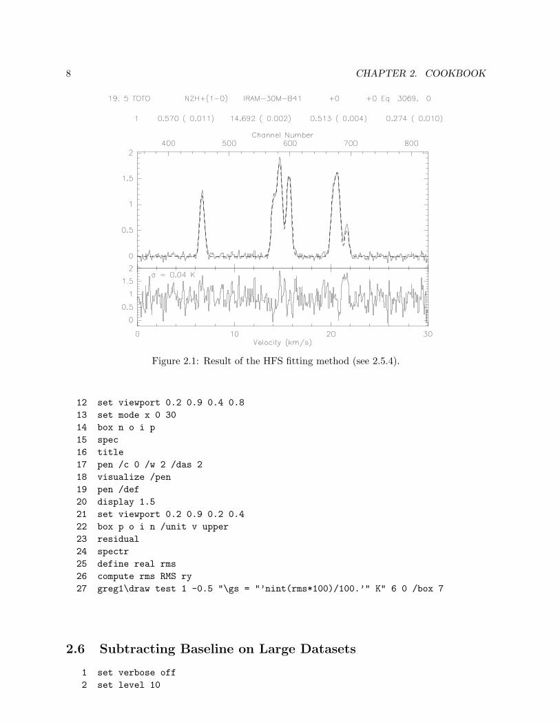
8 CHAPTER 2. COOKBOOK
Figure 2.1: Result of the HFS fitting method (see 2.5.4).
12 set viewport 0.2 0.9 0.4 0.813 set mode x 0 3014 box n o i p15 spec16 title17 pen /c 0 /w 2 /das 218 visualize /pen19 pen /def20 display 1.521 set viewport 0.2 0.9 0.2 0.422 box p o i n /unit v upper23 residual24 spectr25 define real rms26 compute rms RMS ry27 greg1\draw test 1 -0.5 "\gs = "’nint(rms*100)/100.’" K" 6 0 /box 7
2.6 Subtracting Baseline on Large Datasets
1 set verbose off2 set level 10

2.6. SUBTRACTING BASELINE ON LARGE DATASETS 9
3 dev im w4 greg1\set plot portrait5 set format brief6 set angle sec7 file in co21.30m8 find /range -6 6 -6 69 load
10 plot /index11 set window /polygon 112 base 1 /index13 plot /index14 sic rename window-1.pol my-window-1.pol15 sic delete co21-base.30m16 file out co21-base.30m new17 for i 1 to found18 get n19 base 120 write21 next22 file in co21.bas23 find24 load25 plot /index
1. Makes class quiet.
2. Turn off nearly all output messages.
3. Open an image window (necessary to plot 2D images).
4. Change the orientation to portrait.
5. Title in short format.
6. Set arcsecond units.
7. Open the file.
8. Build an index according to offsets.
9. Build a 2D array.
10. Display the whole index.
11. Define a polygon interactively to set spectral windows. By default the polygon is stored ina file window-1.pol.
12. Subtract a 1st order polynom to all records.
13. Display the result.
14. Change the polygon filename (to avoid overwritting it next time).
10 CHAPTER 2. COOKBOOK
15. Delete output file if it exists.
16. Open the output file as new.
17-21 Make a loop over the index to subtract the baseline and write the result.
22-25 Display the result from the output file.
2.7 Reading/Writing FITS file
2.7.1 Exporting class Spectra through FITS
1 set angle sec2 file in co21.30m3 find /range -2 2 -2 24 get f5 set fits mode spectrum6 fits write single.fits7 find /range -2 2 -2 28 fits write index.fits /mode index
1. Angles are expressed in arcseconds.
2. Open the .30m file.
3. Build the index.
4. Store the first spectrum in R memory.
5. Default mode for writing FITS is set to single spectrum.
6. Write the R memory in FITS format file ’single.fits’.
7. Re-build the index.
8. Write the whole index in FITS format file ’index.fits’.
2.7.2 Importing FITS spectra into class
1 set angle sec2 fits read single3 file out single.30m single /overwrite4 write5 file in single.30m6 find7 get f8 plot
1. Angles are expressed in arcseconds.
2. Read a single FITS spectrum.
3-4 Open a new .30m file.

2.7. READING/WRITING FITS FILE 11
3. Write the FITS spectrum in the .30m file.
6-9 Check the result by plotting the spectrum from the .30m file.

12 CHAPTER 2. COOKBOOK

Chapter 3
User manuel
3.1 Generalities
3.1.1 Data and Log Files
class uses two files of data; one for input and one for output, which may be the same actualfile. The input file is only used to read. An observation contains several independent subsections.These file are defined by the command FILE (IN,OUT,BOTH) Filename, possibly followed by NEWif a new file is to be initialized. The default extension of files is .30m. This can be changed withSET EXTENSION .my extension.
class also keeps two log files, named class.log and class.mes. They are created at classstart in the default directory $HOME/.gag/logs. This directory is defined in the sic logicalgag log: which can be customized in the user customization file: $HOME/.gag.dico. The logfiles may be used to keep track of a batch or interactive work.
3.1.2 Observation and Version Number
Within class, an observation should represent a single observing configuration, e.g. a singledirection observed at a single central frequency with a single spectral resolution and in one polar-ization only (i.e. a single sky position, front-end and back-end combination). Each observationis given a number, named observation number at the time of creation of the class data file. Thisnumber is then carried out in further manipulations.
Several version of a given observation may be stored in the same data file. Each version ofa given observation thus represent different stages of the data reduction and all the versions ofa given observation gives the history of the data processing. Each version of an observation isgiven a number (starting at 1), named version number at the time of creation of the class datafile. The version number increases automatically, each time the observation is modified (usingWRITE). By default, only the last version of a given observation is relevant, i.e. GET reads the lastversion of an observation. It is possible (but not recommended) to store an observation withoutincrementing the version number with the UPDATE command so that you can go back to previousstages of reduction in case of big mistakes.
Provided you respect this use of the version number, data reduction can be largely automated.Failing to do this, i.e. using the same observation number for very different things at timeof creation of the class data file, implies that you have to remember yourself which versioncorresponds to which configuration.
13
14 CHAPTER 3. USER MANUEL
3.1.3 Scan and Subscan Number
For bookkeeping purpose, class keeps track of a Scan and a Subscan number, which can be usedas a selection criterium. The Scan number is attributed at observing time which is carried outin the class data format. Moreover, two different observing mode are nowdays in common usein single-dish telescope:
• The pointed observing mode for which the telescope is pointed toward the source directionduring all the integration to obtain only one spectrum. The scan is made of only onespectrum whose intensity is accumulated during the scan duration. Hence the Subscannumber is always 1.
• The On–The–Fly (OTF) observing mode for which the telescope drift on source duringthe integration to make a small map. The scan is here composed of a collection of spectradumped regularly (typically every 1 second) during a contiguous portion of time. Eachdumped spectrum is also tagged by a subscan number whose value is incremented for eachnew OTF line (both to enable easy selection of a single line inside one OTF scan, and toensure consistency with the 30m numbering). This subscan number is foreseen to always begreater than 1. There is one exception: when class read data in old format, the subscannumber is zero and a warning is issued.
3.1.4 Entry Number and Index
The FIND command offers the possibility to build an index of the observations matching severalgiven selection criteria. The user can then easily process consistently only those observations.Each time a new index is formed using the FIND command, all the selected observations (which willbelong to this index) are sequentially attributed a number, named entry number. This numbergoes from 1 to found, the number of observations in the current index. The entry number isnever saved. It is just used as a number to process the current index in a loop.
Default selection criteria are defined by the SET command. For most selection criteria, anoption to the FIND command exists, with the same name, which may be used to impose temporaryvalues to the FIND command; the default values are unchanged by the FIND options.
• SET LINE Name for the line name to be used. A line name of the form ABC* indicates thatall lines beginning by ABC are to be selected. The default is *, i.e. any line name.
• SET NUMBER n1 n2 for the range of observation numbers. Default is * *, i.e. any observa-tion number; * n2 specifies all observation numbers smaller than n2.
• SET OBSERVED d1 d2 for the range of observing dates. A date is specified in the formatdd-mmm-yyyy, e.g. 19-jan-1985. Default is * *, i.e. any date; 19-JAN-1985 * means anydate later than January 19th, 1985.
• SET OFFSET o1 o2 for offsets of the position to be used (in the system and units specifiedby SET COORDINATE and SET ANGLE). Default is * *.
• SET RANGE w e s n is a less restrictive way to specify position offsets. A rectangular areaof sky is defined by its west, east, south and north limits (in current angle units).
• SET REDUCED d1 d2 for a range in reduction dates; same specifications and defaults as forSET OBSERVED.

3.1. GENERALITIES 15
• SET SOURCE Name for the source name; same specifications as SET LINE.
• SET SCAN s1 s2 for a range of original scan numbers. Scan numbers should not be confusedwith Observation numbers (the numbers by which an observation is uniquely identified).They are essentially “history” numbers defined by the acquisition system, but usually withdifferent “observations” (in the class meaning) for a single scan. The scan number is keptonly for bookkeeping purpose.
• SET TELESCOPE Name for the Telescope name. For the IRAM 30-m telescope, the telescopename contains coded into the last 3 letters the backend used for the observations. Similarconventions are used for spectra coming from Plateau de Bure Interferometer.
• SET TYPE Name specifies on which type of observations you deal with: “Continuum”, “Line”or “Skydip”.
The tolerance parameter defined by SET MATCH also influences on the position searches, since thisparameter (in the current angle unit) is used to check agreement with the specified limits. Anotheroption to the FIND command is /ALL which enables to find all the versions of all observationssatisfying the selection criteria (otherwise only the most recent version is selected). Note thatthe system is intended to work only with the last version of observations, so that the use of the/ALL option should remain exceptional.
Finally, the SET SORT force the FIND command to sort all the entries of an index in ascendingorder of a key parameter (e.g. lambda or beta offsets). SET SORT number implies the defaultorder.
3.1.5 R and T Memories
class keeps 2 observations in memory, in two different buffers, called R and T. The R memory isthe only one that may be accessed directly; the T memory is only used for operations on spectra(additions,...). The GET n command places the spectrum corresponding to entry number n in theR buffer, while the previous R content is stored in the T buffer. The command SWAP exchangesboth memories.
3.1.6 Large Set of Spectra
It is today possible with the IRAM–30 m to map a square degree field in CO (2-1). As an orderof magnitude, this gives a final spectra cube of about 106 spectra with a slightly oversampling of4′′. An observer who has just spent a few hours observing the same source in OTF mode maywant to process all the dumped spectra at once even though they do not belong to the same scan.
The LOAD command gathers all the individual spectra currently in the index as a 2D array forfuture work, in particular visualization. This requires that all the spectra currently in the indexare coherent, i.e. same source name, same line name and above all exactly the same frequencysampling. The latter can easily be achieved just by resampling. No checking is currently doneabout this, i.e. this is currently the responsibility of the observer to ensure a coherent frequencyaxis. The /INDEX option of commands like PLOT or BASE modifies there behavior to directly workon the 2D array defined with the LOAD command.
Nota Bene: The STRIP command which is producing a Velocity-Position plots, is obsolescent.Indeed the same functionality can be achived by the combination LOAD; PLOT /INDEX if theindex is correctly choosen. And the LOAD command is much more powerful.
16 CHAPTER 3. USER MANUEL
3.1.7 Variables
The Rope to Hang Yourself
class makes use of sic variables to allow more flexibility in the processing, in particular in proce-dures. sic variables are extremely powerful, with the side effect that if you want, you can corruptyour data by overwriting some information. class attempts to prevent the most disastrous er-rors by defining some of the most critical variables as READONLY. They cannot be overwritten bythe user, but their values can be used in expressions, either arithmetic or logical. However, anunprotected mode is available for specific processing using the command SET VARIABLE.
Index Variables
The variable FOUND refers to the number of observations in the index. It is declared Read-Onlyof course. Its main use is either to write a sic loop that goes through the index or to test foractions which should be performed only if something exists in the index. The FIND commanddoes not return an error, but set FOUND = 0, if it finds nothing. A second variable related tothe index is the INDEX array, of dimension FOUND, which contains the observation numbers of allobservations in the index.
Header Variables
The most important header parameters are defined by default as sic variables in a protectedmode. The others, of less frequent use, can be accessed if required by the user (see “AdvancedProcessing”). The default variables are (RW means Read-Write variable, RO, Read-Only).
TELESCOPE Character*12, RW, Telescope nameNUMBER Integer, RW, Observation numberVERSION Integer, RO, Version numberDATATYPE Integer, RO, Type of observation
0 Line, 1 Continuum, 2 SkydipQUALITY Integer, RO, Quality of dataSCAN Integer, RO, Original scan numberUTOBS Double, RO, UT of observation (Radians)LSTOBS Double, RO, LST of observation (Radians)AZIMUTH Real, RW, Azimuth of observation (Radians)ELEVATION Real, RW, Elevation of observation (Radians)TSYS Real, RW, System temperatureTIME Real, RW, Integration time (Seconds)
SOURCE Character*12, RW, Source nameLAMBDA Double, RW, Longitude of source (Radians)BETA Double, RW, Latitude of source (Radians)OFF_LAMBDA Double, RW, Offset in longitude (Radians)OFF_BETA Double, RW, Offset in latitude (Radians)EQUINOX Real, RW, Equinox of coordinates (Years)
LINE Character*12 RW, Line nameCHANNELS Integer, RO, Number of channelsREFERENCE Real, RW, Reference channel

3.2. SPECTRA LINE PROCESSING 17
FREQ_STEP Real, RW, Frequency step by channel (MHz)VELO_STEP Real, RW, Velocity step by channel (km/s)VELOCITY Real, RW, Velocity of reference channelFREQUENCY Double, RW, Rest frequency at reference channelIMAGE Double, RW, Image frequency " " " "
BEAM_EFF Real, RW, Telescope beam efficiencyFORWARD_EFF Real, RW, Telescope forward efficiencyGAIN_IMAGE Real, RW, Image to signal band ratioWATER Real, RO, Water vapor content (mm)PRESSURE Real, RO, External pressure (hPa)AMBIENT_T Real, RO, External temperature (K)CHOPPER_T Real, RO, Chopper temperature (K)COLD_T Real, RO, Cold load temperature (K)TAU_SIGNAL Real, RO, Opacity in signal bandTAU_IMAGE Real, RO, Opacity in image bandATM_SIGNAL Real, RO, Atmospheric temperature
in signal bandATM_IMAGE Real, RO, Atmospheric temperature
in image band
RX Real[8192] RO, X values of data pointsRY Real[8192] RW, Y values of data points
8192 is currently the maximum size of the spectra, but the variables RX and RY are redimensionedto the effective number of channels for each spectrum.
Advanced Processing
All header parameters can be defined as sic variables for specific processing of the data, eitheras Read-Only or as Read-Write, using the command SET VARIABLE. Read-Write mode is to beused with caution, since even critical variables (e.g. the number of channels) can be modified.Refer to command SET VARIABLE for more details.
By using the appropriate variables and the sic mathematical and logical facilities, customizeddata processing becomes possible, as well as complete data editing.
3.2 Spectra Line Processing
3.2.1 Plotting Spectra
Plotting spectra is controlled by several parameters:
• SET UNIT Type defines the unit of the X axis, which may be C (for Channel number), V(for Velocity), F (for Frequency) or I (for Image).
• SET PLOT Type defines the plotting type PLOT (Normal or Histogram); Normal gives straightlines connecting the data points (this is the default since it is faster). Histogram gives amore realistic representation of spectroscopic data.
18 CHAPTER 3. USER MANUEL
• SET MODE X (or Y) Type defines the plotting limits in X or Y, where type stands for TOTAL(all channels plotted in X, complete scale in Y), AUTO (take the plotting limits in use whenthe spectrum was last written), or two numbers for fixed limits; X or Y specify the axis onwhich the type is to apply. For X axis, the limits are in the current units (C, V or F). ForF, specify the offset from the rest frequency in MHz (note: the caption and the numberson the axis will refer to absolute rest frequencies).
Single spectrum
Single spectrum are usually plotted using the following commands:
• BOX, which plots the frame. The Y axes are labelled in temperature units; the X axes maybe in the following units: Velocity, Frequency, Image frequency, or Channel number. Theupper X axis may be labelled in a different unit than that of the lower axis. Units for bothaxes are entered by the command SET UNIT L U, where L and U stand for the units of lowerand upper axes and may be any of V, F, I, or C. The second parameter U is optional; ifnot entered, it defaults to L.
BOX accepts the option /UNIT which specifies a unit temporarily different from the currentone (given by the SET UNIT command). The parameter UPPER will modify only the unit forthe upper axis of the frame. For instance: BOX /UNIT F UPPER will give velocities on thelower axis (if this is the current unit specified by SET UNIT V) and rest frequencies on theupper axis.
• SPECTRUM, which plots the spectrum, in the current mode, clipped into the current box. Anoffset may be given as argument to plot two spectra above each other for comparison.
• TITLE, which writes a header above the frame. The title format is controlled by theSET FORMAT command.
• PLOT, which performs all of CLEAR; BOX; SPECTRUM; TITLE in a single operation.
Spectra map
Using the MAP command, it is possible to produce a plot of spectra in the current index, arrangedin a map. Use the option /CELL Size x Size y to specify the size of a spectrum, in currentangle units. Without this option a default is taken (the actual separation of the spectra). Option/GRID will produce frames around the spectra. The argument MATCH can be given to fix theaspect ratio of the boxes to the cell sizes.
The map size can be controlled using commands SET PAGE and SET BOX LOCATION. Labelscan be suppressed by option /NOLABEL (and ticks will not be drawn if of size 0.0). Option /NUMBERwill add the observation number with each spectrum.
After the MAP command has been used, the POPUP command may be used to display in anotherwindow a spectrum selected either from its observation number or from its offsets. POPUP can alsobe used after the STAMP command. The STAMP command allows to display many observations atonce, without requesting the X and Y axis scales to be fixed.
Large set of spectra
An efficient way to look at a large set of coherent spectra (e.g. observed in OTF mode) is to plotthem as a 2-D image where the intensity is colour coded. The image is formed by applying the

3.2. SPECTRA LINE PROCESSING 19
LOAD on the current index. Then the /INDEX option modify the single spectra plotting commandsas follow:
• BOX /INDEX, which plots the frame, i.e. the entry number (Y axis) as a function of thevelocity and/or frequency (X axis). The ranges of X and Y axes are controlled by theSET MODE command. SET MODE Y always control the intensity range.
• SPECTRUM /INDEX, which plots the image.
• TITLE /INDEX, which writes a header above the frame. Range of parameters (e.g. scannumber, beta and lambda offsets, ...) are written.
• PLOT /INDEX, which performs all of CLEAR; BOX /INDEX; SPECTRUM /INDEX; TITLE/INDEX in a single operation.
3.2.2 Removing Baselines
The BASE command subtracts polynomial baselines of degree < 30. The fitting algorithm usesChebyshev polynomials, and does not allow any extrapolation outside the fitting range. It isthus important to fit the baseline out to the maximum extension of the wanted spectrum. Ifextrapolation is needed, a constant value will be used outside the fitting range, equal to thepolynom value at the boundary. The algorithm warns if the polynomial degree is too high. Seesection 2.6 for a typical baseline fitting session.
The user first defines line windows by the command SET WINDOW with the following syntax:
SET WINDOW [wl1 wu1 [wl2 wu2 [...]]] [/VAR array][/POLYGON [N] [filename1...filenameN]][/NOCURSOR]
The POLYGON option enable the definition of 2D polygons on images obtain with LOAD; PLOT/INDEX when working on all the index. Line window values may be entered numerically asarguments, red from variables and line polygons may be red from input files. If available, thecursor may be used to define the windows or polygons. In the window case, enter the values inthe same order as above by typing “N” or “ ” (space bar); “C” cancels the last value entered;“H” types a help message and “E” terminates the operation. In the case of polygons, each leftclic defines a gon and a right clic terminates the operations. The polygons may leak out of theimage. Several polygons may be defined in case the line appear at very different velocities.
Up to 100 windows or 5 polygons may be defined. BASE then fits a polynomial to the partof the spectrum outside the line windows. However, only the “visible” parts of the spectrum areused and bad channels are taken out. The degree of the polynomial is defined by SET BASE n, ortemporarily by the BASE command itself with its argument.
Sinusoidal baselines may also be subtracted, using the command BASE SINUS AmplitudePeriod Phase where Amplitude, Period and Phase are initial guesses for a minimization routine.A linear baseline is added to the sinusoid in any case.
When working on an individual spectrum (not the index), the /PLOT option plots the fittedbaseline in the current box. The area in the windows as well as the rms noise, are computed.A baseline can be computed for one spectrum, and then subtracted from a different one usingBASE LAST. This may be helpful for example at Pico-Veleta where you may remove from the 100kHz backend the baseline determined from the 1 MHz one. Be sure that you do not change theX-unit between the time you computed the baseline and the time you remove it...

20 CHAPTER 3. USER MANUEL
When working on the whole index, the baseline are fitted spectrum per spectrum and thebaseline–corrected spectra are stored in the 2D array ready for plotting with the next PLOT/INDEX command. However, baseline fitting results are lost and an explicit loop on the indexentry must be use including a new baseline computation) to store the results with the WRITEcommand.
3.2.3 Folding Frequency Switched Spectra
Spectra obtained by Frequency Switching need to be folded to obtain the source spectra. It isusually a good idea to remove a baseline before the spectra are folded in order to use as muchbaseline as possible. The folding is done by command FOLD which reads from the correspondingsection all the necessary parameters. FOLD only operates on the R buffer. The number of channelsis decreased to keep only the relevant part of the resulting spectrum.
3.2.4 Adding Spectra
Four parameters define the way spectra are added. These are the align mode, the combinationmode, the integration weighting, and the behaviour with respect to bad channels.
Four alignment modes are available, by the means of the command SET ALIGN Mode:
• CHANNEL in which spectra are added channel by channel. This is only useful when thespectra have been obtained in strictly identic conditions. Warning messages are given whenthis is not the case.
• VELOCITY in which the velocity scale is used to align the spectra. This enables you to addspectra of different origin. An interpolation is performed if needed. If individual spectrahave differing spectral resolutions, the lowest spectral resolution is used for the result.
• FREQUENCY in which the rest frequency is used to align the spectra.
• POSITION, in which continuum drifts are aligned regarding to the position along the drift.
CHANNEL, VELOCITY and FREQUENCY are relevant for Line observations, while POSITION is relevantonly for Continuum observations. Two combination modes are possible with the command SETALIGN MODE Combination:
• INTERSECT where only the intersection of individual spectra is kept.
• COMPOSITE where the reunion of the individual spectra is kept (as in a spectral scan forexample).
Three weighting types may be used, with the command SET WEIGHT Type:
• TIME for weights proportional to the observing time, divided by the square of the systemnoise.
• SIGMA for weighting by the inverse square of the rms noise of each individual spectrum.
• NONE or EQUAL for equal weighting. Caution: equal weighting behaves differently inAVERAGE and ACCUMULATE commands. AVERAGE produces the average of spectra, whileACCUMULATE gives the sum of the two spectra. After division by the number of addedspectra, ACCUMULATE will thus give the same result as AVERAGE.
3.2. SPECTRA LINE PROCESSING 21
Bad channels are dealt with in two possible ways, defined by the command SET BAD Mode:
• OR where resulting channels are declared bad if they were declared as such in at least oneof the individual spectra.
• AND where resulting channels are declared bad if they were bad in all individual spectra.
Default values are ALIGN CHANNEL INTERSECT, WEIGHT TIME, and BAD OR.Two other parameters control whether summing spectra is allowed or not. Positions are
checked according to SET MATCH Tolerance or SET NOMATCH. If (absolute) positions differ bymore than the tolerance parameter, an error message is generated. The tolerance is spec-ified in current angle units. The homogeneity of the calibration is checked according tothe SET CALIBRATION Beam Tolerance Gain Tolerance or SET CALIBRATION OFF commands.Beam Tolerance is the maximum difference allowed in the beam efficiencies to add spectra (de-fault 0.02) and Gain Tolerance the maximum difference between the gains in the image band(default 0, which means not checked).
There are two ways of adding spectra: the commands AVERAGE and ACCUMULATE. AVERAGEoperates globally on all the spectra in the index, while ACCUMULATE adds the R and T buffers into R.AVERAGE is generally better for systematic methods, ACCUMULATE for special cases. The drawbackof ACCUMULATE is in the need for initialization; one needs a spectrum in T and a spectrum in R tobegin with...
3.2.5 Analyzing profiles
The class user may analyse spectra by fitting profiles. The fitting commands are availablefrom the FIT language. The minimization method is taken from the MINUIT system of CERN,modified and optimized for this purpose. Reliability proved to be good. Five types of profiles arepresently available, and can be selected by the METHOD command:
• METHOD GAUSS This is the default type of profile. One may use up to five Gaussians, whichmight depend on each other as specified by a system of control codes associated with eachvariable. For each of these Gaussians, the primary parameters are: 1) Area, 2) Position,and 3) Width (FWHM). The current X unit (for the lower axis) is used. Code 0 meansthat the parameter is adjustable; 1 that it is fixed; 2 that the parameter (head of group)is adjustable and that another parameter, coded 3, is fixed with respect to it; 4 that theparameter is a fixed head of group.
• METHOD SHELL (see details below) Profiles are like those encountered in envelopes of stars.The primary parameters are Area, Position, Width and Horn to Center ratio. The aspectof the profile varies from parabola (as obtain in optically thick lines) for Horn/Center= -1 to flat-topped lines (unresolved optically thin lines) for Horn/Center = 0 and doublepeaked profiles (resolved optically thin lines) for Horn/Center > 0. The profile is symmetric.Presently only code 0 and 1 can be used, and up to 5 independent lines can be fitted in asingle spectrum. The X unit must be frequency.
• METHOD NH3(1,1) or NH3(2,2) or NH3(3,3)Profiles taking into account hyperfine structure of ammonia with a Gaussian distribution ofvelocity are fitted. Primary variables are 1) The product (Main Group Opacity) times (Ex-citation Temperature minus Background Temperature) 2) Velocity 3) Line Width (FWHM)and 4) Main Group Opacity . Up to 3 independent lines can be fitted, and only codes 0and 1 are allowed. The X unit must be Velocity.

22 CHAPTER 3. USER MANUEL
• METHOD HFS FileName This method is similar to the previous one, but the HyperFineStructure parameters are read from a file instead of being known by class . The first lineof this file must contain the number of hyperfine components (< 40). The other lines mustcontain, for each component, the velocity offset and the relative intensity. The parametersare the same as for NH3 method.
• METHOD CONTINUUM This method is used for continuum drifts. It fits a Gaussian and alinear baseline in the drift. If beam-switching was used and the reference beam is along thedrift direction, two dependent Gaussian are used to optimize signal to noise. The methoddoes not require any user input.
METHOD SHELL in details. The fitted function is:
f(ν) =A
∆ν1 + 4H [(ν − ν0)/∆ν]2
1 +H/3
where the fitted parameters are:
1. A: the area under the profile (in K MHz),
2. ν0: the middle frequency (in MHz),
3. ∆ν: the full width at zero level (in MHz),
4. H: the Horn/Center parameter (dimensionless, see below)
The central value is f(ν0) = A∆ν
11+H/3 whilst the value at the edge is f(ν0+∆ν/2) = A
∆ν1+H
1+H/3 .The edge-to-center intensity ratio value is thus dictated by the Horn/Center parameter H ac-cording to
f(∆ν/2)f(0)
= 1 +H
The center-to-edge frequency shift corresponds to an expanding velocity
vexp = c∆ν/2ν0
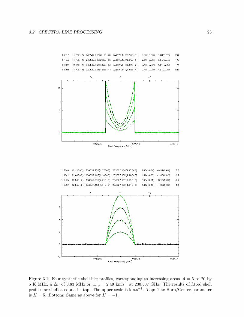
Figure 3.1 shows synthetic shell-like profiles, for which the area takes values A = 5 to 20 by5 K MHz. The full width at zero level is ∆ν = 3.83 MHz in all cases, which corresponds tovexp = 2.49 km.s−1at 230.537 GHz. The Horn/Center parameter is H = 5 (top) or H = −1(bottom, for which the intensity at the edge is zero).
The FIT commands are:
• LINES N defines the number of components and prompts for the initial values of the param-eters for each component. This command has no effect for method CONTINUUM. Parametersare read in list directed format in the following order:
Code, Intensity, Code, Position, Code, Width, [Code, Parameter 4]
The code is an integer number between 0 and 4. Note that, though the program works onthe area (or other quantities as for NH3 methods), you have to give the intensity, since thisquantity is more intuitive than area. The use of the list directed format makes things easier
3.2. SPECTRA LINE PROCESSING 23
Figure 3.1: Four synthetic shell-like profiles, corresponding to increasing areas A = 5 to 20 by5 K MHz, a ∆ν of 3.83 MHz or vexp = 2.49 km.s−1at 230.537 GHz. The results of fitted shellprofiles are indicated at the top. The upper scale is km.s−1. Top: The Horn/Center parameteris H = 5. Bottom: Same as above for H = −1.

24 CHAPTER 3. USER MANUEL
when only one parameter has to be modified (cf Fortran norms). The number of lines Nmay be zero; in this case the program finds out reasonable starting values by itself.
Values may be also entered graphically if the cursor is available. After entering LINES N,first point the cursor to one side of the line, strike one key, point the cursor the other side,strike another key. The program computes the moment of the spectrum between theseboundaries and use it to set up starting values. Proceed like this for all components. Onedrawback of this way of entering values is that you cannot change the control codes. Itshould be used only for entirely independent and free lines.
• MINIMIZE activates minimization, then prints out the results after convergence. A Simplexmethod is first used to ensure convergence, then a Gradient method to refine the results,and compute the errors.
• ITERATE is similar to MINIMIZE, but starts from the previous minimization results. Only theGradient method is used. Consequently, this command is only useful close to the minimum.
• VISUALIZE [N] [/PEN] plots the Nth component obtained by fitting; if N is not given, thesum of all components is plotted.
• RESIDUAL N subtracts the Nth component from the current spectrum, or the sum of allcomponents is N is not given). In this process, the R spectrum is first copied into T, thenthe difference is done in R.
• DISPLAY Prints the results of fitting from the current spectrum, without recomputing it ...
• KEEP Saves the fit results in the input file, which must be opened also for output. KEEP isin fact a reduced version of UPDATE, and to be used with the same care as UPDATE.
• SET MASK ... Defines masks in the spectrum for the fit. This commands has the samesyntax and behaviour as SET WINDOW. Masked regions will not be used for the fit.
Fit results are always saved by a WRITE command and made available through the correspondingvariable section (see SET VARIABLE help).
3.2.6 Gridding Spectra on a 3-D Data Cube
See memo IRAM 2005-1 (CLASS evolution: I. Improved OFT support) available herehttp://iram-institute.org/medias/uploads/class-evol1.pdf
3.2.7 Miscellaneous
• DIVIDE makes the ratio of the R and T spectra. The two spectra must have the same velocityscale.
• FFT plots the power spectrum of the current observation. It might help identify spuriousripples. Editing of the fourier transform is possible, so that these ripples may be suppressed.
• NOISE generates a Gaussian noise as intense as in the current spectrum using the rms valuedetermined by the BASE command, or using a rms value given as an argument. NOISEValue NEW will create a noisy spectrum of given noise level into R, after copying R in T.
3.3. CONTINUUM AND SKYDIP PROCESSING 25
• RESAMPLE resamples the R spectrum on the specified grid. If the final sampling is coarserthan the original one, a smoothing occurs to the final sampling.
• SMOOTH operates a Hanning smoothing by default and divide the number of channels by two.Other arguments can be specified to use other methods. SMOOTH AUTO uses a sophisticatedvariable-resolution algorithm, but it requires the channels to be really independent andthis is apparently seldom the case in radio astronomy. SMOOTH GAUSS Width convolves thespectrum by Gaussian of given Width in current units; it does not take care of bad channels.SMOOTH BOX N make the average of N adjacent channels and divides the number of channelsby N.
3.3 Continuum and Skydip Processing
3.3.1 Continuum
So far, we have handled only Spectroscopic data, but Continuum data can be processed by class. Currently, only continuum drifts can be reduced. The basic idea is to treat continuum driftsas spectra would be. Accordingly, very few commands behave differently in Continuum andSpectroscopy modes.
Continuum mode is accessed by typing the SET TYPE CONTINUUM command. The prompt thenchanges to CAS> (Continuum Analysis System). You can return to Spectroscopy mode later ontyping the SET TYPE SPECTROSCOPY or LINE command and the prompt changes to LAS> (LineAnalysis System).
Some commands have slightly different behaviour in Spectroscopy and Continuum modes.
• SET UNIT has no effect in Continuum mode.
• SET ANGLE also controls the plotting units in Continuum mode.
• METHOD: only GAUSS and CONTINUUM methods are allowed in Continuum mode.
• LINES has no effect with CONTINUUM method.
• HEADER uses a different format for Continuum and Spectroscopy modes.
• STRIP produces a map from a set of parallel drifts. The index must define such a set ofdrifts.
• FITS format support is experimental for continuum data.
• With CONTINUUM method, PRINT FIT command only outputs a single component, and thecomponent number is not written.
• SET ALIGN CHANNELS and SET ALIGN POSITION are the only available alignment modes inContinuum mode.
Except for these restrictions, the behaviour of other commands is similar. Note that commandFIND only selects data of the current type.

26 CHAPTER 3. USER MANUEL
3.3.2 Skydip Processing
class is able to reduce skydip data. Skydip mode must be selected using command SET MODESKYDIP which also changes the prompt to SAS> (Skydip Analysis System). Commands FIND,HEADER, GET, PLOT and WRITE may be used as for Continuum and Line modes, but the only othervalid command is REDUCE which fits the sky emission using atmospheric information available inthe data, and displays the results.
3.4 Communication with the outer world
3.4.1 Listing Scientifically Valuable Results
Command PRINT offers a way to list a number of valuable information on screen or in anASCII/binary file:
• PRINT FIT, which prints the results of profile fits. For each spectrum, N lines are written(N being the number of fitted components), and each line contains in the following order(1) the component number, (2) then observation number, (3,4) the two cartography offsets,(5,6) area of Gaussian and corresponding error, (7,8) same for position, (9,10) same forwidth, (11) intensity, (12,13) rms on the baseline and on the line. Offset are in the currentcoordinate system and units. The current method is used.
For Continuum method, only a single Gaussian is written. The written information isoriented towards pointing measurements: (1) the observation number (2,3) Azimuth andelevation (4,5) area of Gaussian and error, (6,7) position, (8,9) width, (10) intensity, (11,12)rms on baseline and signal, (13,14) collimations. All angular values are in the current angleunit. The values are followed by the source name.
• PRINT AREA, prints the area of the line computed by the BASE command. Each line contains(1,2) offsets, (3) area, (4) rms noise. PRINT AREA V1 V2 V3 V4 ..., prints areas withinvelocity slices (if such is the current X unit, but one could use channels or frequencies).Ranges are V1-V2, V2-V3, V3-V4, ... etc. Each line will contain (1,2) the offsets, followedby the areas in order.
• PRINT CHANNEL List, prints values of channels in the list. The list is specified in the FORn1 TO n2 BY n3 format. Total number of channels is however limited to 15.
• PRINT MOMENT V1 V2 V3 V4 ..., prints moments (area, position, width), of the datawithin the velocity (or channels or frequencies, depending on the current units) V1-V2,V3-V4, etc... Each line contains (1,2) the offsets, (3,4,5) the moments for V1-V2, (6,7,8)for V3-V4 etc...
• PRINT POINTING, prints results of CONTINUUM method fits printed in a format adaptedto pointing constants measurements. The output is suited for further processing and de-termination of pointing constants using the point program.
• PRINT FLUX, prints results of CONTINUUM method fits printed in a format adapted toflux determination. The output is suited for further processing using the flux program.
As all commands using a set of spectra, PRINT works on the whole current index. Output is bydefault printed on the screen, but may be directed onto a file by the /OUTPUT Filename option.

3.4. COMMUNICATION WITH THE OUTER WORLD 27
Alternatively, the same information may be written to a “Table” (a special kind of gildasimage). The Table format is much faster and suppresses some of the limitations of the format-ted output on the number of columns written. Table format is obtained using option /TABLETablename.
3.4.2 Making Publishable Quality Figures
class has many functionalities to directly produce publishable quality Figures. All the gregcommands are imported in class to fully annotate plots, superpose spectra with related data,stack various plots and then make hardcopy (like Post-Scripts files). A few guidelines are givenhere on essential greg commands. For more details, users are advised to read the greg manual.
Moreover, class commands like DRAW and GREG implements fancy functionalities of commonuse when producing figures around spectra.
greg functionalities
class is mainly used for interactive look at spectra, hence its default values are all orientedtowards fast plotting on screen. These defaults can be changed by command SET. If the value ofa parameter is not controlled by class, the command will be passed on to greg for processing.
The following greg presentation parameters are useful:
• SET BOX LOCATION It can be set to LANDSCAPE, PORTRAIT, SQUARE or 4 numbers indicat-ing the position of the box in the plot page (in centimeters).
• SET CHARACTER Size Control the size of characters in centimeters.
• SET FONT Quality Select the character quality to be used, SIMPLEX or DUPLEX. The fontsare identical to the ones used by greg , and the character handling is the same (in commandDRAW TEXT).
• SET PLOT PAGE ... Define the page size. Warning: You will get into trouble if you wantto abreviate this command to SET PLOT as SET PLOT is a valid class command used toindicate whether spectra are broken lines of histograms. A way out of this is to abbreviatethe greg command as G\SET PLOT.
• SET TICK Size Define the tick size in centimeters.
Note that you do not need to open a plotting window to produce a hardcopy through theHARDCOPY command. It is only much more convenient, but the plot (e.g. sequence of commands)and the way it is displayed (e.g. PS format, bitmap on a computer screen) are two completelyindependent things.
Bridge toward greg functionalities
The spectra and the results of their analysis (like the fits) are in class internal buffers notalways easily accessible for plotting with the greg commands. class thus implements the GREGcommand which is intended to produce a direct interface with greg for plots of spectra. It createsa gildas table which can be read using the standard greg commands for further plotting. Thetable contains the following columns for Spectra:

28 CHAPTER 3. USER MANUEL
1. Intensity2. Channel number3. Velocity4. Offset frequency5. Rest frequency6. Image frequency7. Fitted profiles if any - fit(i),i=0,nline - in column 7+i,
for the current method.
The output table can be put later in a formatted way using gildas task LIST if needed. Forcontinuum data, the table contains
1. Intensity2. Channel number3. Angular offset (radian)4. Fitted profile if any.
The table may be used as input to greg to produce fancy plots, or by the gildas softwarefor other applications. In particular, the sic monitor (command LET) is able to subtract any ofthe fits from the spectrum to produce residuals if needed. It is possible to merge different tables,add columns to a table, etc... For example, from two spectra at the same velocity resolution itis possible to merge the two tables and compute the ratio of the spectra, as well as the errors onthis ratio.
Annotations
class has two DRAW commands to annotate plots: i) The standard greg DRAW command whichcan be accessed by typing G\DRAW (please look at the greg manual) and ii a special flavor ofDRAW customized for annotating spectra. The class flavor is the default one used when typingjust DRAW The basic operations performed by this flavor of the DRAW command are:
• DRAW TEXT Xpos Ypos "Text" Centering to draw a text at position (Xpos,Ypos) (in cur-rent units) with the specified centering code. This command works more or less like thegreg command of same name. Please refer to the greg manual for details. In particular,you can include Greek letters and Symbols in the text using the escape character \. Astrange thing may appear on the screen, but it is O.K. on the plot.
• DRAW UPPER Xpos "Text" to draw a vertically oriented text at position Xpos, with a verticalline connecting the beginning of the text to the current spectrum. This text and line arewritten at position Xpos, in units of the upper axis. Typically, this command is used tomark spectral line identifications.
• DRAW LOWER Xpos "Text" same as above, but with Xpos in units of the lower axis.
• DRAW WINDOW [Level] shows the current line windows by marks on the graphic plot. Levelis an optional arguments indicating at what Y value the marker should be put (Default 0).
• DRAW MASK [Level] same as above but for the current masks.
• DRAW KILL [Channel] kills the specified channel (current one if using the cursor) by at-tributing it the “blanking” or “undefined” value.
3.4. COMMUNICATION WITH THE OUTER WORLD 29
• DRAW FILL [Channel] Fills the specified channel (current one if using the cursor) by in-terpolation between the nearest non-blanked channels. The channel must have been killedbefore.
Any other character will not draw anything, but simply returns the cursor position, with corre-sponding values of the velocity, frequency, image frequency, channel number.
3.4.3 Importing and Exporting Spectra From and To FITS
No data reduction package has all the functionalities any user dream about. But a user mayknow that the functionality he needs is available in a very specific package. Here comes the needto exchange data between packages. The current standard answer to this problem is FITS. classto FITS conversion (and vice-versa) is done by command FITS. In addition, all functionalitiesprovided by the sic command DEFINE FITS are of course available. For a description of the FITSformat see the original paper by Wells et al. (Astron. and Astrophys. Suppl.).
The class FITS command has the following syntax:
FITS READ Filename[.fits]
to read a FITS file and create class data from it, or
FITS WRITE Filename[.fits] [/BITS Nbits] [/MODE SPECTRUM|INDEX]
to write a FITS file from class data.In addition, default values can be supplied by the SET FITS command.
SET FITS BITS NbitsSET FITS MODE Spectrum|Index|None
From FITS to CLASS
FITS READ Filename[.fits]
will read a FITS file and create class data from it. It is expected to work under the followingconditions:
1. The Filename.fits file contains one spectrum, with (a subset of) the FITS keywords whichare described in the previous section. FITS Keyword redefinition is possible.
2. OR The Filename.fits contains a BINTABLE, also with recognized FITS keywords.
3. No more, no less
This may look akwardly restrictive, but is already powerful if you have thought about your datadestination when creating the FITS file.
FITS Keyword redefinition
A minimal number of keywords has been defined as part of the FITS standard, but additionalones can be (and have been) added by various groups to support their own needs. Thus, several“flavors” of FITS coexist. A detailed description of the class FITS flavors is given in chapter 4.Unknown keywords are normally ignored, but class supports FITS keyword redefinition. Ifyou receive a file with scan number coded as NUMBER (instead of SCAN-NUM), all you need todo is to define a SIC symbol named NUMBER with translation SCAN-NUM. This is done by typingSIC\SYMBOL NUMBER SCAN-NUM.

30 CHAPTER 3. USER MANUEL
From class to FITS
To write a FITS file from class data, use the following command:
FITS WRITE Filename[.fits] [/BITS Nbits] [/MODE SPECTRUM|INDEX]
The command will create a simple FITS file from the current Spectrum (in SPECTRUM mode),or a FITS BINTABLE from the current Index (in INDEX mode). The number of bits can becontrolled. Default values for the mode and the number of bits can be supplied by the SET FITScommand.
SET FITS BITS NbitsSET FITS MODE Spectrum|Index|None
In INDEX mode, it is up to the user to make sure that the index is consistent (same number ofchannels, etc..., for all spectra in index).

Chapter 4
Developer Manual (16-sep-2015)
Please check directly the class sources to get the most up-to-date information.
4.1 Internal class Format
The class Data Format is built upon the Classic Data Container. Please refer to the dedicateddocumentation for details.
4.1.1 Contents of one observation
Data, i.e. observational parameters as well as spectra, is organized in the following way:
• One observation is self-contained. All the information needed to reduce it is recorded onthe same few disk blocks. It may be one spectrum or one continuum drift.
• Each observation is divided in several sections, containing header parameters or data:
– General information (date, times, local coordinates, sequence number, ...)
– Positional information (source, name, astronomical coordinates, equinox, offsets, ...)
– Spectral information (number of spectra, line names ans frequencies, resolutions, num-ber of channels, ...)
– Data
– ...
In the Classic nomenclature, one observation is saved into one entry in a Classic file. Eachentry is composed of an entry descriptor + the observation itself (header+intensity array). Pleaserefer to the section The File Entries in the Classic documentation for details about the way anentry is written in the file.
4.1.2 File organization
class files strictly respect the Classic Data Container specifications (see the dedicated documen-tation for details). In particular, the file identification codes (first 4 bytes) are described in thisdocumentation. class files use the kind 1 in the File Descriptor.
31

32 CHAPTER 4. DEVELOPER MANUAL (16-SEP-2015)
4.1.3 File index
The Entry Indexes, gathered into Extension Indexes, are ruled by the Classic Data Containerspecifications. According to these, the index contents are let free to Class. They are describedbelow for files version 1 and 2.
Table 4.1: Index version 1 (found in files version 1). Note that index length is 32 words (so that4 of them fit in a 128 words record), even if 10 words are left unused.
Position Parameter Fortran Kind Unit Purpose1 bloc Integer*4 Record Record where observation is to be found2 num Integer*4 Observation number3 ver Integer*4 Observation version
4-6 csour Character*12 Source name7-9 cline Character*12 Line name
10-12 ctele Character*12 Telescope name13 dobs Integer*4 GAG date Observation date14 dred Integer*4 GAG date Reduction date15 off1 Real*4 Radian Lambda offset16 off2 Real*4 Radian Beta offset17 type Integer*4 Code Coordinate system18 kind Integer*4 Code Kind of data19 qual Integer*4 Code Quality of data20 scan Integer*4 Scan number21 posa Real*4 Radian Position angle (drifts)22 subscan Integer*4 Subscan number
23-32 (unused) Padding to 32 words

4.2. THE HEADER AND DATA SECTIONS 33
Table 4.2: Index version 2 (found in files version 2)
Position Parameter Fortran Kind Unit Purpose1-2 bloc Integer*8 Record Record where observation is to be found3 word Integer*4 Word Word where the obs. starts in this record
4-5 num Integer*8 Observation number6 ver Integer*4 Observation version
7-9 csour Character*12 Source name10-12 cline Character*12 Line name13-15 ctele Character*12 Telescope name
16 dobs Integer*4 GAG date Observation date17 dred Integer*4 GAG date Reduction date18 off1 Real*4 Radian Lambda offset19 off2 Real*4 Radian Beta offset20 type Integer*4 Code Coordinate system21 kind Integer*4 Code Kind of data22 qual Integer*4 Code Quality of data23 posa Real*4 Radian Position angle (drifts)
24-25 scan Integer*8 Scan number26 subscan Integer*4 Subscan number
4.2 The Header and Data Sections
Here we describe the contents of the main header sections (excerpts from the storage declarationsin the class program itself). Note that, in the data file, the actual length of some of the sectionsis variable, e.g. the length of the switching information section depends on the number of differentphases in the switching procedure.
4.2.1 General Parameters
! GENERAL: General parameters, always present.integer(kind=4), parameter :: class_sec_gen_id=-2integer(kind=4), parameter :: class_sec_gen_len=9type general
sequence! Written in the index on diskinteger(kind=4) :: num ! [ ] Observation numberinteger(kind=4) :: ver ! [ ] Version numberinteger(kind=4) :: teles(3)! [ ] Telescope nameinteger(kind=4) :: dobs ! [MJD-60549] Date of observationinteger(kind=4) :: dred ! [MJD-60549] Date of reductioninteger(kind=4) :: kind ! [ code] Type of datainteger(kind=4) :: qual ! [ code] Quality of datainteger(kind=4) :: scan ! [ ] Scan numberinteger(kind=4) :: subscan ! [ ] Subscan number! Written in the section on disk

34 CHAPTER 4. DEVELOPER MANUAL (16-SEP-2015)
real(kind=8) :: ut ! [ rad] UT of observationreal(kind=8) :: st ! [ rad] LST of observationreal(kind=4) :: az ! [ rad] Azimuthreal(kind=4) :: el ! [ rad] Elevationreal(kind=4) :: tau ! [neper] Opacityreal(kind=4) :: tsys ! [ K] System temperaturereal(kind=4) :: time ! [ s] Integration timeinteger(kind=4) :: xunit ! [ code] X unit (if X coordinates section is present)
end type general
4.2.2 Position information
Observation version 2 since 26-mar-2015:
! POSITION: Position information.integer(kind=4), parameter :: class_sec_pos_id=-3integer(kind=4), parameter :: class_sec_pos_len=14type position
sequenceinteger(kind=4) :: sourc(3) ! [ ] Source nameinteger(kind=4) :: system ! [code] Coordinate systemreal(kind=4) :: equinox ! [year] Equinox of coordinatesinteger(kind=4) :: proj ! [code] Projection systemreal(kind=8) :: lam ! [ rad] Lambda of projection centerreal(kind=8) :: bet ! [ rad] Beta of projection centerreal(kind=8) :: projang ! [ rad] Projection anglereal(kind=4) :: lamof ! [ rad] Offset in Lambdareal(kind=4) :: betof ! [ rad] Offset in Beta
end type position
Observation version 1 (obsolete for writing):
! POSITION: Position information.integer(kind=4), parameter :: class_sec_pos_id=-3integer(kind=4), parameter :: class_sec_pos_len=17type position
sequenceinteger(kind=4) :: sourc(3) ! [ ] Source namereal(kind=4) :: equinox ! [year] Equinox of coordinatesreal(kind=8) :: lam ! [ rad] Lambdareal(kind=8) :: bet ! [ rad] Betareal(kind=4) :: lamof ! [ rad] Offset in Lambdareal(kind=4) :: betof ! [ rad] Offset in Betainteger(kind=4) :: proj ! [code] Projection systemreal(kind=8) :: sl0p ! [ rad] lambda of descriptive systemreal(kind=8) :: sb0p ! [ rad] beta of descriptive systemreal(kind=8) :: sk0p ! [ rad] angle of descriptive system
end type position

4.2. THE HEADER AND DATA SECTIONS 35
4.2.3 Spectroscopic information (for spectra)
Observation version 1.3 (Doppler correction added, SkyFr and Vteles removed):
! SPECTRO: Spectroscopic information (for spectra).integer(kind=4), parameter :: class_sec_spe_id=-4integer(kind=4), parameter :: class_sec_spe_len=17type spectro
sequenceinteger(kind=4) :: line(3) ! [ ] Line namereal(kind=8) :: restf ! [ MHz] Rest frequencyinteger(kind=4) :: nchan ! [ ] Number of channelsreal(kind=4) :: rchan ! [ ] Reference channelreal(kind=4) :: fres ! [ MHz] Frequency resolutionreal(kind=4) :: foff ! [ MHz] Frequency offsetreal(kind=4) :: vres ! [km/s] Velocity resolutionreal(kind=4) :: voff ! [km/s] Velocity at reference channelreal(kind=4) :: bad ! [ ] Blanking valuereal(kind=8) :: image ! [ MHz] Image frequencyinteger(kind=4) :: vtype ! [code] Type of velocityreal(kind=8) :: doppler ! [km/s] Doppler correction -V/c (CLASS convention)
end type spectro
Observation version 1.2 (SkyFr and Vteles added), obsolete for writing:
! SPECTRO: Spectroscopic information (for spectra).integer(kind=4), parameter :: class_sec_spe_id=-4integer(kind=4), parameter :: class_sec_spe_len=18type spectro
sequenceinteger(kind=4) :: line(3) ! [ ] Line namereal(kind=8) :: restf ! [ MHz] Rest frequencyinteger(kind=4) :: nchan ! [ ] Number of channelsreal(kind=4) :: rchan ! [ ] Reference channelsreal(kind=4) :: fres ! [ MHz] Frequency resolutionreal(kind=4) :: foff ! [ MHz] Frequency offsetreal(kind=4) :: vres ! [km/s] Velocity resolutionreal(kind=4) :: voff ! [km/s] Velocity at reference channelreal(kind=4) :: bad ! [ ] Blanking valuereal(kind=8) :: image ! [ MHz] Image frequencyinteger(kind=4) :: vtype ! [code] Type of velocityreal(kind=8) :: skyfr ! [ MHz]real(kind=4) :: vteles ! [km/s]
end type spectro
Observation version 1.1, obsolete for writing:
! SPECTRO: Spectroscopic information (for spectra).integer(kind=4), parameter :: class_sec_spe_id=-4

36 CHAPTER 4. DEVELOPER MANUAL (16-SEP-2015)
integer(kind=4), parameter :: class_sec_spe_len=15type spectro
sequenceinteger(kind=4) :: line(3) ! [ ] Line namereal(kind=8) :: restf ! [ MHz] Rest frequencyinteger(kind=4) :: nchan ! [ ] Number of channelsreal(kind=4) :: rchan ! [ ] Reference channelsreal(kind=4) :: fres ! [ MHz] Frequency resolutionreal(kind=4) :: foff ! [ MHz] Frequency offsetreal(kind=4) :: vres ! [km/s] Velocity resolutionreal(kind=4) :: voff ! [km/s] Velocity at reference channelreal(kind=4) :: bad ! [ ] Blanking valuereal(kind=8) :: image ! [ MHz] Image frequencyinteger(kind=4) :: vtype ! [code] Type of velocity
end type spectro
4.2.4 Baseline information (for spectra or drifts)
! BASE: Baseline information (for spectra of drifts).integer(kind=4), parameter :: class_sec_bas_id=-5integer(kind=4), parameter :: mwind=100integer(kind=4), parameter :: class_sec_bas_len=8+2*mwindtype base
sequenceinteger(kind=4) :: deg ! [ ] Degree of last baselinereal(kind=4) :: sigfi ! [Int. unit] Sigmareal(kind=4) :: aire ! [Int. unit] Area under windowsinteger(kind=4) :: nwind ! [ ] Number of line windowsreal(kind=4) :: w1(mwind) ! [ km/s] Lower limits of windowsreal(kind=4) :: w2(mwind) ! [ km/s] Upper limits of windowsreal(kind=4) :: sinus(3) ! [ ] Sinus baseline results
end type base
4.2.5 Scan numbers of initial observations
! HISTORY: Scan numbers of initial observations.integer(kind=4), parameter :: class_sec_his_id=-6integer(kind=4), parameter :: mseq=100integer(kind=4), parameter :: class_sec_his_len=2*mseq+1type history
sequenceinteger(kind=4) :: nseq ! Number of sequencesinteger(kind=4) :: start(mseq) ! Start can number of seq.integer(kind=4) :: end(mseq) ! End scan number of seq.
end type history
4.2.6 Default plotting limits
! PLOT: Default plotting limits.
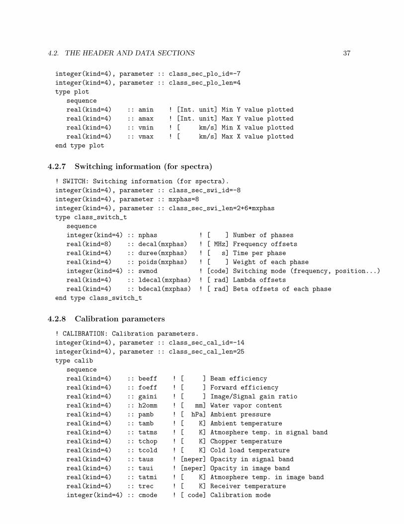
4.2. THE HEADER AND DATA SECTIONS 37
integer(kind=4), parameter :: class_sec_plo_id=-7integer(kind=4), parameter :: class_sec_plo_len=4type plot
sequencereal(kind=4) :: amin ! [Int. unit] Min Y value plottedreal(kind=4) :: amax ! [Int. unit] Max Y value plottedreal(kind=4) :: vmin ! [ km/s] Min X value plottedreal(kind=4) :: vmax ! [ km/s] Max X value plotted
end type plot
4.2.7 Switching information (for spectra)
! SWITCH: Switching information (for spectra).integer(kind=4), parameter :: class_sec_swi_id=-8integer(kind=4), parameter :: mxphas=8integer(kind=4), parameter :: class_sec_swi_len=2+6*mxphastype class_switch_t
sequenceinteger(kind=4) :: nphas ! [ ] Number of phasesreal(kind=8) :: decal(mxphas) ! [ MHz] Frequency offsetsreal(kind=4) :: duree(mxphas) ! [ s] Time per phasereal(kind=4) :: poids(mxphas) ! [ ] Weight of each phaseinteger(kind=4) :: swmod ! [code] Switching mode (frequency, position...)real(kind=4) :: ldecal(mxphas) ! [ rad] Lambda offsetsreal(kind=4) :: bdecal(mxphas) ! [ rad] Beta offsets of each phase
end type class_switch_t
4.2.8 Calibration parameters
! CALIBRATION: Calibration parameters.integer(kind=4), parameter :: class_sec_cal_id=-14integer(kind=4), parameter :: class_sec_cal_len=25type calib
sequencereal(kind=4) :: beeff ! [ ] Beam efficiencyreal(kind=4) :: foeff ! [ ] Forward efficiencyreal(kind=4) :: gaini ! [ ] Image/Signal gain ratioreal(kind=4) :: h2omm ! [ mm] Water vapor contentreal(kind=4) :: pamb ! [ hPa] Ambient pressurereal(kind=4) :: tamb ! [ K] Ambient temperaturereal(kind=4) :: tatms ! [ K] Atmosphere temp. in signal bandreal(kind=4) :: tchop ! [ K] Chopper temperaturereal(kind=4) :: tcold ! [ K] Cold load temperaturereal(kind=4) :: taus ! [neper] Opacity in signal bandreal(kind=4) :: taui ! [neper] Opacity in image bandreal(kind=4) :: tatmi ! [ K] Atmosphere temp. in image bandreal(kind=4) :: trec ! [ K] Receiver temperatureinteger(kind=4) :: cmode ! [ code] Calibration mode

38 CHAPTER 4. DEVELOPER MANUAL (16-SEP-2015)
real(kind=4) :: atfac ! [ ] Applied calibration factorreal(kind=4) :: alti ! [ m] Site elevationreal(kind=4) :: count(3) ! [count] Power of Atm., Chopp., Coldreal(kind=4) :: lcalof ! [ rad] Longitude offset for sky measurementreal(kind=4) :: bcalof ! [ rad] Latitude offset for sky measurementreal(kind=8) :: geolong ! [ rad] Geographic longitude of observatoryreal(kind=8) :: geolat ! [ rad] Geographic latitude of observatory
end type calib
4.2.9 For Skydips observations. No associated data.
! SKYDIP: For Skydips observations. No associated data.integer(kind=4), parameter :: class_sec_sky_id=-16integer(kind=4), parameter :: msky=10integer(kind=4), parameter :: class_sec_sky_len=10+4*mskytype skydip
sequenceinteger(kind=4) :: line(3) ! [ ] Line namereal(kind=8) :: restf ! [MHz] Rest frequencyreal(kind=8) :: image ! [MHz] Image frequencyinteger(kind=4) :: nsky ! [ ] Number of points on skyinteger(kind=4) :: nchop ! [ ] - - - - chopperinteger(kind=4) :: ncold ! [ ] - - - - cold loadreal(kind=4) :: elev(msky) ! [rad] Elevationsreal(kind=4) :: emiss(msky) ! [ ?] Power on skyreal(kind=4) :: chopp(msky) ! [ ?] Power on chopperreal(kind=4) :: cold(msky) ! [ ?] Power on cold load
end type skydip
4.2.10 Gauss fit results (for spectra or drifts)
! GAUSS: Gauss fit results (for spectra or drifts).integer(kind=4), parameter :: class_sec_gau_id=-9integer(kind=4), parameter :: mxgaus=5integer(kind=4), parameter :: mgausfit=3*mxgausinteger(kind=4), parameter :: class_sec_gau_len=3+2*mgausfittype gauss
sequenceinteger(kind=4) :: nline ! [ ] Number of componentsreal(kind=4) :: sigba ! [ Int. unit] Sigma on basereal(kind=4) :: sigra ! [ Int. unit] Sigma on linereal(kind=4) :: nfit(mgausfit) ! [area,v0,fwhm] Fit resultsreal(kind=4) :: nerr(mgausfit) ! [area,v0,fwhm] Errors
end type gauss
4.2.11 ”Stellar shell” profile fit results (for spectra)
! SHELL: "Stellar shell" profile fit results (for spectra).integer(kind=4), parameter :: class_sec_she_id=-12

4.2. THE HEADER AND DATA SECTIONS 39
integer(kind=4), parameter :: mshellfit=20integer(kind=4), parameter :: class_sec_she_len=3+2*mshellfittype shell
sequenceinteger(kind=4) :: nline ! [] Number of componentsreal(kind=4) :: sigba ! [] Sigma on basereal(kind=4) :: sigra ! [] Sigma on linereal(kind=4) :: nfit(mshellfit) ! [] Fit resultsreal(kind=4) :: nerr(mshellfit) ! [] Errors
end type shell
4.2.12 Hyperfine structure profile fit results (for spectra)
! HFS: "Hyperfine Structure" profile fit results (e.g. NH3, HCN, for spectra).integer(kind=4), parameter :: class_sec_hfs_id=-13integer(kind=4), parameter :: mhfsfit=12integer(kind=4), parameter :: class_sec_hfs_len=3+2*mhfsfittype hfs
sequenceinteger(kind=4) :: nline ! Number of componentsreal(kind=4) :: sigba ! Sigma on basereal(kind=4) :: sigra ! Sigma on linereal(kind=4) :: nfit(mhfsfit) ! Fit resultsreal(kind=4) :: nerr(mhfsfit) ! Errors
end type hfs
4.2.13 Hyperfine structure absorption profile fit results (for spectra)
! ABS: "Hyperfine Structure" absorption profile fit results (e.g. NH3, HCN, for spectra).integer(kind=4), parameter :: class_sec_abs_id=-18 ! Absorption fitinteger(kind=4), parameter :: mabsfit=16integer(kind=4), parameter :: class_sec_abs_len=3+2*mabsfittype absorption
sequenceinteger(kind=4) :: nline ! Number of componentsreal(kind=4) :: sigba ! Sigma on basereal(kind=4) :: sigra ! Sigma on linereal(kind=4) :: nfit(mabsfit) ! Fit resultsreal(kind=4) :: nerr(mabsfit) ! Errors
end type absorption
4.2.14 Continuum drift description (for drifts)
! DRIFT: Continuum drift description (for drifts).integer(kind=4), parameter :: class_sec_dri_id=-10integer(kind=4), parameter :: class_sec_dri_len=16type drift
sequencereal(kind=8) :: freq ! [ MHz] Rest frequency

40 CHAPTER 4. DEVELOPER MANUAL (16-SEP-2015)
real(kind=4) :: width ! [ MHz] Bandwidthinteger(kind=4) :: npoin ! [ ] Number of data pointsreal(kind=4) :: rpoin ! [ ] Reference pointreal(kind=4) :: tref ! [ ?] Time at referencereal(kind=4) :: aref ! [ rad] Angular offset at ref.real(kind=4) :: apos ! [ rad] Position angle of driftreal(kind=4) :: tres ! [ ?] Time resolutionreal(kind=4) :: ares ! [ rad] Angular resolutionreal(kind=4) :: bad ! [ ] Blanking valueinteger(kind=4) :: ctype ! [code] Type of offsetsreal(kind=8) :: cimag ! [ MHz] Image frequencyreal(kind=4) :: colla ! [ ?] Collimation error Azreal(kind=4) :: colle ! [ ?] Collimation error El
end type drift
4.2.15 Beam-switching parameters (for spectra or drifts)
! BEAM: Beam-switching parameters (for spectra or drifts).integer(kind=4), parameter :: class_sec_bea_id=-11integer(kind=4), parameter :: class_sec_bea_len=5type beam
sequencereal(kind=4) :: cazim ! [ rad] Azimuth of observationreal(kind=4) :: celev ! [ rad] Elevation of observationreal(kind=4) :: space ! [ rad] Beam spacingreal(kind=4) :: bpos ! [ rad] Position angle of beamsinteger(kind=4) :: btype ! [code] System for angle
end type beam
4.2.16 Double gaussian and baseline fit results (for drifts)
! CONTINUUM: Double gaussian and baseline fit results (for drifts).integer(kind=4), parameter :: class_sec_poi_id=-15integer(kind=4), parameter :: mpoifit=8integer(kind=4), parameter :: class_sec_poi_len=3+2*mpoifittype pointing
sequenceinteger(kind=4) :: nline ! Number of componentsreal(kind=4) :: sigba ! Sigma on basereal(kind=4) :: sigra ! Sigma on linereal(kind=4) :: nfit(mpoifit) ! Fit resultsreal(kind=4) :: nerr(mpoifit) ! Errors
end type pointing
4.2.17 Herschel Space Observatory (HIFI)
integer(kind=4), parameter :: class_sec_her_id=-20integer(kind=4), parameter :: class_sec_her_len=96type class_herschel_t
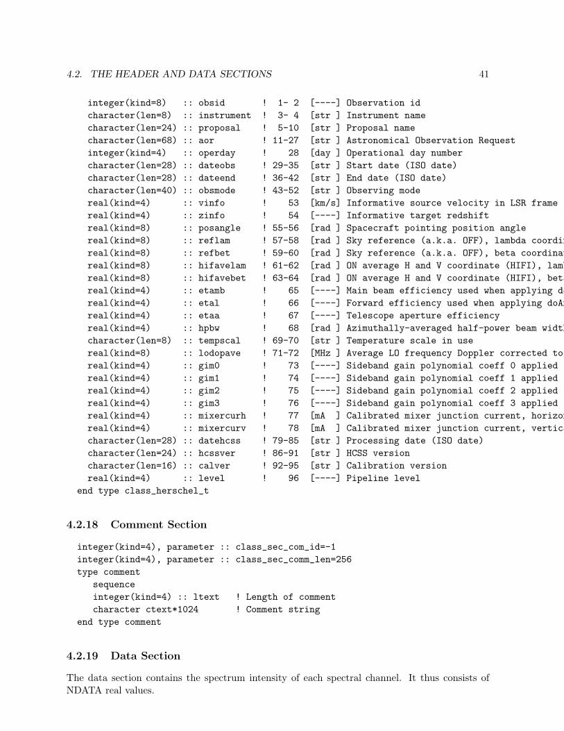
4.2. THE HEADER AND DATA SECTIONS 41
integer(kind=8) :: obsid ! 1- 2 [----] Observation idcharacter(len=8) :: instrument ! 3- 4 [str ] Instrument namecharacter(len=24) :: proposal ! 5-10 [str ] Proposal namecharacter(len=68) :: aor ! 11-27 [str ] Astronomical Observation Requestinteger(kind=4) :: operday ! 28 [day ] Operational day numbercharacter(len=28) :: dateobs ! 29-35 [str ] Start date (ISO date)character(len=28) :: dateend ! 36-42 [str ] End date (ISO date)character(len=40) :: obsmode ! 43-52 [str ] Observing modereal(kind=4) :: vinfo ! 53 [km/s] Informative source velocity in LSR framereal(kind=4) :: zinfo ! 54 [----] Informative target redshiftreal(kind=8) :: posangle ! 55-56 [rad ] Spacecraft pointing position anglereal(kind=8) :: reflam ! 57-58 [rad ] Sky reference (a.k.a. OFF), lambda coordinatereal(kind=8) :: refbet ! 59-60 [rad ] Sky reference (a.k.a. OFF), beta coordinatereal(kind=8) :: hifavelam ! 61-62 [rad ] ON average H and V coordinate (HIFI), lambda coordinatereal(kind=8) :: hifavebet ! 63-64 [rad ] ON average H and V coordinate (HIFI), beta coordinatereal(kind=4) :: etamb ! 65 [----] Main beam efficiency used when applying doAntennaTempreal(kind=4) :: etal ! 66 [----] Forward efficiency used when applying doAntennaTempreal(kind=4) :: etaa ! 67 [----] Telescope aperture efficiencyreal(kind=4) :: hpbw ! 68 [rad ] Azimuthally-averaged half-power beam widthcharacter(len=8) :: tempscal ! 69-70 [str ] Temperature scale in usereal(kind=8) :: lodopave ! 71-72 [MHz ] Average LO frequency Doppler corrected to freqFrame (SPECSYS)real(kind=4) :: gim0 ! 73 [----] Sideband gain polynomial coeff 0 appliedreal(kind=4) :: gim1 ! 74 [----] Sideband gain polynomial coeff 1 appliedreal(kind=4) :: gim2 ! 75 [----] Sideband gain polynomial coeff 2 appliedreal(kind=4) :: gim3 ! 76 [----] Sideband gain polynomial coeff 3 appliedreal(kind=4) :: mixercurh ! 77 [mA ] Calibrated mixer junction current, horizontalreal(kind=4) :: mixercurv ! 78 [mA ] Calibrated mixer junction current, verticalcharacter(len=28) :: datehcss ! 79-85 [str ] Processing date (ISO date)character(len=24) :: hcssver ! 86-91 [str ] HCSS versioncharacter(len=16) :: calver ! 92-95 [str ] Calibration versionreal(kind=4) :: level ! 96 [----] Pipeline level
end type class_herschel_t
4.2.18 Comment Section
integer(kind=4), parameter :: class_sec_com_id=-1integer(kind=4), parameter :: class_sec_comm_len=256type comment
sequenceinteger(kind=4) :: ltext ! Length of commentcharacter ctext*1024 ! Comment string
end type comment
4.2.19 Data Section
The data section contains the spectrum intensity of each spectral channel. It thus consists ofNDATA real values.

42 CHAPTER 4. DEVELOPER MANUAL (16-SEP-2015)
4.3 Old OTF data format
This section is kept for backward compatibility. Indeed class is still able to read old OTF dataformat. Once class, always class...
4.3.1 Data Section Descriptor
! Data Section Descriptor.! (Old OTF data format, kept for backward compatibility).integer(kind=4), parameter :: class_sec_desc_id=-30integer(kind=4), parameter :: class_sec_desc_len=4type descriptor
sequenceinteger(kind=4) :: ndump ! Number of recordsinteger(kind=4) :: ldpar ! Length of data header (longwords)integer(kind=4) :: ldatl ! length of line data (")integer(kind=4) :: ldump ! length of record (")integer(kind=4) :: rec ! Current Record Number
end type descriptor
4.3.2 Multiple spectra Data Section
A multiple spectra data section contains many spectra, obtained in a single observing scan:typically a drift scan across a source, a on-off scan with a multi-beam receiver, or a drift scanwith a multi-beam receiver. The data section is considered as a multiple spectra data section is thespecial section ‘Data Section Descriptor’ is present. It consists of a R_NDUMP records (individualspectra); each spectrum has R_LDATL line channels, and is followed by a few data associatedparameters (R_LDPAR words). The length of each record is thus R_LDUMP=R_LDPAR+R_LDATL; thetotal length of the data section should be: NDATA=R_NDUMP*R_LDUMP.
The data header presently contains:
offset type name0 Integer*4 Record number1 Real*4 AZ [rad] Telescope Azimuth2 Real*4 EL [rad] Telescope Elevation3 Real*8 ST [rad] Sideral Time5 Real*4 LAMOF [rad] Azimuth offset6 Real*4 BETOF [rad] Elevation offset12 Real*4 UT [sec] Universal Time in day DOBS
4.4 class FITS format
Starting with dec06 release of gildas, the FITS support of class is largely improved. In additionto the old possibility of writing one spectrum per file (see the “Simple SPECTRUM Mode” sec-tion), it is now possible to read from the same FITS file, one spectrum in the primary Header/DataUnit and collections of spectra in bintables stored as FITS extensions (see the “BINTABLEMode”). Moreover, it is now possible to store in the same bintable, spectra of different number of

4.4. CLASS FITS FORMAT 43
channels. The distinction between the SPECTRUM and BINTABLE mode is mainly historicalas the software automatically toggles from one mode to another.
4.4.1 Simple SPECTRUM Mode
FITS headers written by class depend on the informations present in the corresponding classheaders. Any missing information will also be omitted in FITS (and vice versa). A typical FITSheader written by class looks like this :
SIMPLE = T /BITPIX = 16 /NAXIS = 4 / (1)NAXIS1 = 253 / (2)NAXIS2 = 1 / (3)NAXIS3 = 1 / (3)NAXIS4 = 1 / (3)BSCALE = 0.1038147092913E-03 /BZERO = -0.2413805246353E+01 /DATAMIN = -0.5815605640411E+01 /DATAMAX = 0.9877878427505E+00 /BUNIT = ’K ’ / (4)CTYPE1 = ’FREQ ’ / (5)CRVAL1 = 0.0000000000000E+00 / Offset frequencyCDELT1 = 0.1000000014901E+06 / Frequency resolutionCRPIX1 = 0.1345000000000E+03 /CTYPE2 = ’RA ’ / (6)CRVAL2 = 0.8388750229169E+02 /CDELT2 = -0.5555555975722E-02 /CRPIX2 = 0.0000000000000E+00 /CTYPE3 = ’DEC ’ / (6)CRVAL3 = -0.1777777752148E+01 /CDELT3 = 0.0000000000000E+00 /CRPIX3 = 0.0000000000000E+00 /CTYPE4 = ’STOKES ’ / (7)CRVAL4 = 1.0000000000000 /CDELT4 = 0.0000000000000 /CRPIX4 = 0.0000000000000 /TELESCOP= ’IRAM-30M-B20’ /OBJECT = ’ORI-I-2 ’ /GLAT = 0.0000000000000E+00 / Galactic latitude (8)GLON = 0.0000000000000E+00 / Galactic longitude (8)EPOCH = 0.1950000000000E+04 / (9)BLANK = 0.9878914356232E+00 / Blanking valueLINE = ’* ’ / Line name (10)RESTFREQ= 0.1152712040000E+12 / Rest frequency (11)VLSR = 0.1300000000000E+05 / Velocity of ref. channel (12)DELTAV = -0.2600757479668E+03 / Velocity resolution (13)IMAGFREQ= 0.1074062118530E+12 / Image frequency (14)
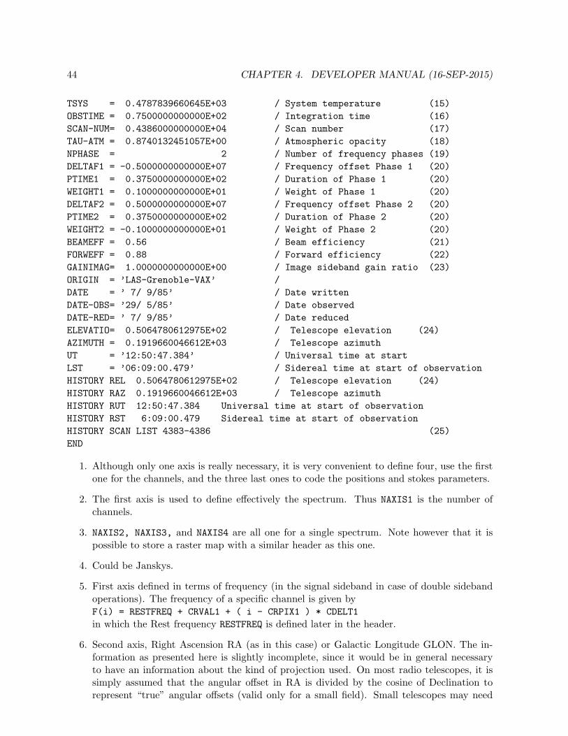
44 CHAPTER 4. DEVELOPER MANUAL (16-SEP-2015)
TSYS = 0.4787839660645E+03 / System temperature (15)OBSTIME = 0.7500000000000E+02 / Integration time (16)SCAN-NUM= 0.4386000000000E+04 / Scan number (17)TAU-ATM = 0.8740132451057E+00 / Atmospheric opacity (18)NPHASE = 2 / Number of frequency phases (19)DELTAF1 = -0.5000000000000E+07 / Frequency offset Phase 1 (20)PTIME1 = 0.3750000000000E+02 / Duration of Phase 1 (20)WEIGHT1 = 0.1000000000000E+01 / Weight of Phase 1 (20)DELTAF2 = 0.5000000000000E+07 / Frequency offset Phase 2 (20)PTIME2 = 0.3750000000000E+02 / Duration of Phase 2 (20)WEIGHT2 = -0.1000000000000E+01 / Weight of Phase 2 (20)BEAMEFF = 0.56 / Beam efficiency (21)FORWEFF = 0.88 / Forward efficiency (22)GAINIMAG= 1.0000000000000E+00 / Image sideband gain ratio (23)ORIGIN = ’LAS-Grenoble-VAX’ /DATE = ’ 7/ 9/85’ / Date writtenDATE-OBS= ’29/ 5/85’ / Date observedDATE-RED= ’ 7/ 9/85’ / Date reducedELEVATIO= 0.5064780612975E+02 / Telescope elevation (24)AZIMUTH = 0.1919660046612E+03 / Telescope azimuthUT = ’12:50:47.384’ / Universal time at startLST = ’06:09:00.479’ / Sidereal time at start of observationHISTORY REL 0.5064780612975E+02 / Telescope elevation (24)HISTORY RAZ 0.1919660046612E+03 / Telescope azimuthHISTORY RUT 12:50:47.384 Universal time at start of observationHISTORY RST 6:09:00.479 Sidereal time at start of observationHISTORY SCAN LIST 4383-4386 (25)END
1. Although only one axis is really necessary, it is very convenient to define four, use the firstone for the channels, and the three last ones to code the positions and stokes parameters.
2. The first axis is used to define effectively the spectrum. Thus NAXIS1 is the number ofchannels.
3. NAXIS2, NAXIS3, and NAXIS4 are all one for a single spectrum. Note however that it ispossible to store a raster map with a similar header as this one.
4. Could be Janskys.
5. First axis defined in terms of frequency (in the signal sideband in case of double sidebandoperations). The frequency of a specific channel is given byF(i) = RESTFREQ + CRVAL1 + ( i - CRPIX1 ) * CDELT1in which the Rest frequency RESTFREQ is defined later in the header.
6. Second axis, Right Ascension RA (as in this case) or Galactic Longitude GLON. The in-formation as presented here is slightly incomplete, since it would be in general necessaryto have an information about the kind of projection used. On most radio telescopes, it issimply assumed that the angular offset in RA is divided by the cosine of Declination torepresent “true” angular offsets (valid only for a small field). Small telescopes may need

4.4. CLASS FITS FORMAT 45
more elaborate projection systems. In the current example, the position really observed isDec = CRVAL3 + ( 1 - CRPIX3 ) * CDELT3Ra = CRVAL2 + ( 1 - CRPIX2 ) * CDELT2 / COS(Dec)That is, CDELT2 and CDELT3 represents angular offsets from the reference position(CRVAL2,CRVAL3) in a Global Sinusoidal projection (RADIO projection).
7. Stokes parameters as defined in the basic paper of Wells et al.
8. Galactic latitude and longitude of the reference position, i.e. of the position(CRVAL2,CRVAL3). If one was using galactic coordinates instead of equatorial ones, theRA and DEC would appear here instead.
9. Equinox of these coordinates.
10. Molecular line name, for bookkeeping.
11. Rest frequency.
12. LSR Velocity of the reference channel. Heliocentric velocities can be used also.
13. Velocity spacings of the channels. This information is duplicate with the rest frequencyand frequency spacing of channels, but convenient. The velocity of a given channel is thusgiven byV(i) = VLSR + ( i - CRPIX1 ) * DELTAV
14. Image frequency, for double sideband operation.
15. System temperature, necessary for some kind of weighting when adding a number of spectra.
16. Integration time, used for the same reason as above.
17. Scan number, for bookkeeping.
18. Atmospheric opacity in the signal sideband.
19. For multi-phased spectra (i.e. frequency switching) number of phases.
20. For each phase, the frequency offset, the phase length and weight.
21. The telescope beam efficiency.
22. The telescope forward efficiency.
23. The ratio of gains in the image and signal sidebands (in case of double sideband operation).
24. Some “History” comments. Whether this information should be given with specific key-words or in an History record is still an open question. This information is not really neededfor further data reduction, but it helps bookkeeping.
25. The list of scan numbers of the spectra added to produce this one.
The FITS interface for Continuum data is still experimental. Try it, and send your com-ments...

46 CHAPTER 4. DEVELOPER MANUAL (16-SEP-2015)
4.4.2 BINTABLE Mode
In addition to the simple “one FITS file per Spectrum” mode, class supports the Binary Tableextension, in reading and writing. class reads and processes all the Binary Table extension ofthe FITS file. The FITS keywords for the Binary Table format are similar to those of the simpleSpectrum mode, but a complete set of spectra can be handled in a single binary table.
Keywords which would change from one spectrum to the next are handled as Binary columnsof the table, with the TTYPEi FITS keyword holding the name of the corresponding simple FITSkeyword. Reading such FITS files, class will support any value for the TTYPEi keywords. If acolumn and a keyword have the same name, the column prevails. If several columns have thesame name (try to avoid this), the last one prevails.
The spectra are handled in a SPECTRUM column.Here is an example with a tiny primary Header Data Unit and a Binary Table extension
header.
SIMPLE = TBITPIX = 8NAXIS = 0EXTEND = TBLOCKED = TORIGIN = ’My observatory’CREATOR = ’Me ’END
...
XTENSION= ’BINTABLE’BITPIX = 8 / Always 8.NAXIS = 2 / Always 2: tables have 2 dimensions.NAXIS1 = 7275 / Number of bytes per row.NAXIS2 = 4 / Number of rows.PCOUNT = 0 / Usually 0.GCOUNT = 1 / Always 1.TFIELDS = 18 / Number of columns.EXTNAME = ’MATRIX ’ / Just a name, not important.EXTVER = 1 / Always 1.MAXIS = 4 / Number of dimensions in the data.MAXIS1 = 1793 / Dummy number of channels (see TTYPE1).MAXIS2 = 1 /MAXIS3 = 1 /MAXIS4 = 1 /CTYPE1 = ’FREQ ’ / Dim1: freq => MAXIS1 = Nb channels.CRVAL1 = 0.0000000000000E+00 / Frequency offset, always 0.CDELT1 = 0.1000000000000E+07 / Frequency resolution [Hz].CRPIX1 = 0.2565000000000E+03 / Dummy reference channel (see TTYPE18).CTYPE2 = ’RA ’CRVAL2 = 0.0000000000000E+00CDELT2 = 0.0000000000000E+00CRPIX2 = 0.0000000000000E+00
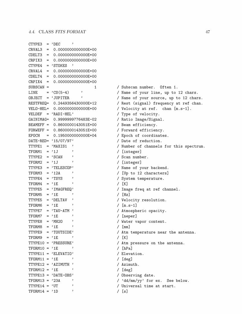
4.4. CLASS FITS FORMAT 47
CTYPE3 = ’DEC ’CRVAL3 = 0.0000000000000E+00CDELT3 = 0.0000000000000E+00CRPIX3 = 0.0000000000000E+00CTYPE4 = ’STOKES ’CRVAL4 = 0.0000000000000E+00CDELT4 = 0.0000000000000E+00CRPIX4 = 0.0000000000000E+00SUBSCAN = 1 / Subscan number. Often 1.LINE = ’CS(5-4) ’ / Name of your line, up to 12 chars.OBJECT = ’JUPITER ’ / Name of your source, up to 12 chars.RESTFREQ= 0.2449356430000E+12 / Rest (signal) frequency at ref chan.VELO-HEL= 0.0000000000000E+00 / Velocity at ref. chan [m.s-1].VELDEF = ’RADI-HEL’ / Type of velocity.GAINIMAG= 0.9999999776483E-02 / Ratio Image/Signal.BEAMEFF = 0.8600000143051E+00 / Beam efficiency.FORWEFF = 0.8600000143051E+00 / Forward efficiency.EPOCH = 0.1950000000000E+04 / Epoch of coordinates.DATE-RED= ’15/07/97’ / Date of reduction.TTYPE1 = ’MAXIS1 ’ / Number of channels for this spectrum.TFORM1 = ’1J ’ / [integer]TTYPE2 = ’SCAN ’ / Scan number.TFORM2 = ’1J ’ / [integer]TTYPE3 = ’TELESCOP’ / Name of your backend.TFORM3 = ’12A ’ / [Up to 12 characters]TTYPE4 = ’TSYS ’ / System temperature.TFORM4 = ’1E ’ / [K]TTYPE5 = ’IMAGFREQ’ / Image freq at ref channel.TFORM5 = ’1E ’ / [Hz]TTYPE5 = ’DELTAV ’ / Velocity resolution.TFORM6 = ’1E ’ / [m.s-1]TTYPE7 = ’TAU-ATM ’ / Atmospheric opacity.TFORM7 = ’1E ’ / [neper]TTYPE8 = ’MH2O ’ / Water vapor content.TFORM8 = ’1E ’ / [mm]TTYPE9 = ’TOUTSIDE’ / Atm temperature near the antenna.TFORM9 = ’1E ’ / [K]TTYPE10 = ’PRESSURE’ / Atm pressure on the antenna.TFORM10 = ’1E ’ / [hPa]TTYPE11 = ’ELEVATIO’ / Elevation.TFORM11 = ’1E ’ / [deg]TTYPE12 = ’AZIMUTH ’ / Azimuth.TFORM12 = ’1E ’ / [deg]TTYPE13 = ’DATE-OBS’ / Observing date.TFORM13 = ’23A ’ / ’dd/mm/yy’ for ex. See below.TTYPE14 = ’UT ’ / Universal time at start.TFORM14 = ’1D ’ / [s]
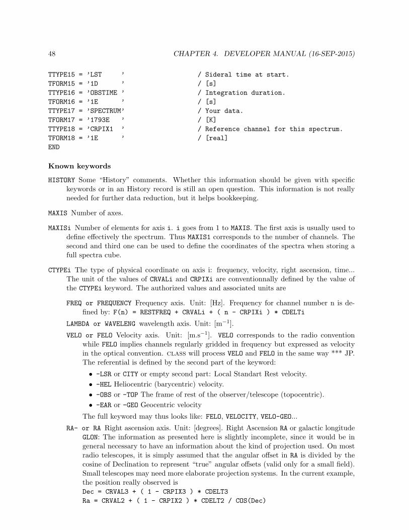
48 CHAPTER 4. DEVELOPER MANUAL (16-SEP-2015)
TTYPE15 = ’LST ’ / Sideral time at start.TFORM15 = ’1D ’ / [s]TTYPE16 = ’OBSTIME ’ / Integration duration.TFORM16 = ’1E ’ / [s]TTYPE17 = ’SPECTRUM’ / Your data.TFORM17 = ’1793E ’ / [K]TTYPE18 = ’CRPIX1 ’ / Reference channel for this spectrum.TFORM18 = ’1E ’ / [real]END
Known keywords
HISTORY Some “History” comments. Whether this information should be given with specifickeywords or in an History record is still an open question. This information is not reallyneeded for further data reduction, but it helps bookkeeping.
MAXIS Number of axes.
MAXISi Number of elements for axis i. i goes from 1 to MAXIS. The first axis is usually used todefine effectively the spectrum. Thus MAXIS1 corresponds to the number of channels. Thesecond and third one can be used to define the coordinates of the spectra when storing afull spectra cube.
CTYPEi The type of physical coordinate on axis i: frequency, velocity, right ascension, time...The unit of the values of CRVALi and CRPIXi are conventionnally defined by the value ofthe CTYPEi keyword. The authorized values and associated units are
FREQ or FREQUENCY Frequency axis. Unit: [Hz]. Frequency for channel number n is de-fined by: F(n) = RESTFREQ + CRVALi + ( n - CRPIXi ) * CDELTi
LAMBDA or WAVELENG wavelength axis. Unit: [m−1].
VELO or FELO Velocity axis. Unit: [m.s−1]. VELO corresponds to the radio conventionwhile FELO implies channels regularly gridded in frequency but expressed as velocityin the optical convention. class will process VELO and FELO in the same way *** JP.The referential is defined by the second part of the keyword:
• -LSR or CITY or empty second part: Local Standart Rest velocity.• -HEL Heliocentric (barycentric) velocity.• -OBS or -TOP The frame of rest of the observer/telescope (topocentric).• -EAR or -GEO Geocentric velocity
The full keyword may thus looks like: FELO, VELOCITY, VELO-GEO...
RA- or RA Right ascension axis. Unit: [degrees]. Right Ascension RA or galactic longitudeGLON: The information as presented here is slightly incomplete, since it would be ingeneral necessary to have an information about the kind of projection used. On mostradio telescopes, it is simply assumed that the angular offset in RA is divided by thecosine of Declination to represent “true” angular offsets (valid only for a small field).Small telescopes may need more elaborate projection systems. In the current example,the position really observed isDec = CRVAL3 + ( 1 - CRPIX3 ) * CDELT3Ra = CRVAL2 + ( 1 - CRPIX2 ) * CDELT2 / COS(Dec)

4.4. CLASS FITS FORMAT 49
DEC- or DEC Declination axis. Unit: [degrees]. Same caveats as for RA.
GLAT Galactic latitude axis. Unit: [degrees]. Same caveat as for RA.
GLON Galactic longitude axis. Unit: [degrees]. Same caveat as for RA.
TIME or UT or UTC Time axis. Unit: [s]. The time since DATE-OBS.
STOKES Stokes axis. The Stokes parameter of the data as defined in the basic paper ofWells et al.
CRPIXi The array location of the reference pixel along axis i. CRPIXi’s value may be a fractionalnumber of pixels and/or outside of the limits of the array. This descriptor is optional fordegenerated axes (i.e. 0 or 1 element).
CRVALi The value of the physical coordinate on axis i at the reference pixel.
CDELTi The increment in physical coordinates along axis i. This descriptor is optional for de-generated axes. Warning: Although there is a difference between the frequency spacingbetween channels and the frequency resolution of each channel, class currently handlesonly one value for both.
BSCALE A value of 1 is assumed when it is undefined. The following formula will be applied tothe FITS data: CLASS_spectrum = BZERO + BSCALE * FITS_spectrum
BZERO A value of 0 is assumed when it is undefined. The following formula will be applied to theFITS data: CLASS_spectrum = BZERO + BSCALE * FITS_spectrum
DATAMIN Minimum value of your spectrum. Understood by class but unused.
DATAMAX Maximum value of your spectrum. Understood by class but unused.
BLANK Blanking value. If not specified, -1e38 assumed. BSCALE and BZERO are applied to theblanking value.
PCOUNT Usually 0. But if you provide your data as Variable Length arrays, then you will haveto tweak this value which specifies the size of the variable length array heap, plus a gap (ifany). See THEAP.
GCOUNT Always 1 in Binary tables.
THEAP Byte offset of heap area. The heap area is where the Variable Length Array data arestored. They are usually stored just after the binary table. The heap does not need tobegin at the end of the main table data. The user may choose to provide a gap between themain table and the beginning of the heap. The size of this gap, in bytes, can be found usingthe value of the THEAP keyword. If there is no gap, the value of THEAP is NAXIS1 * NAXIS2.If there is, the size of the gap is the difference between the value of THEAP and NAXIS1 *NAXIS2. A value of NAXIS1 * NAXIS2 is assumed when this keyword is not defined.
BEAMEFF The main-beam efficiency.
FORWEFF or ETAFSS The forward spillover and scattering efficiency.
GAINIMAG Ratio Image/Signal.
MH2O Water vapor content. Unit: [mm].

50 CHAPTER 4. DEVELOPER MANUAL (16-SEP-2015)
PRESSURE The ambiant atmospheric pressure. Unit: [hPa].
TOUTSIDE The ambient temperature. Unit [K].
NPHASE Value: from 1 to 8. For multi-phased spectra (i.e. frequency switching) number ofphases.
DELTAFj Frequency offset for phase j. Unit: [Hz].
PTIMEj Duration of phase j. Unit: [s].
WEIGHTj Weight of phase j.
TELESCOP A string value giving the telescope name. class truncates this string to the first12 characters. There is a class convention about TELESCOP, which is not mandatory:TELESCOP contains the name of the instrument, the name of the backend and the name ofthe subband (if any). For example: “HIFI-HRV-02” for subband 2 of the High ResolutionSpectrometer (Vertical polarization) of HIFI (one of the Herschel’s instrument).
AZIMUTH The azimuth at TIME. Unit: [degrees]. If the TIME axis is non-degenerated, then this isthe azimuth at the TIME of the first pixel on the TIME axis.
ELEVATIO The elevation at TIME. Unit: [degrees]. Same caveat as for AZIMUTH.
DATE-OBS or DATE_OBS A string giving the observation date and optionally the time at theobservation start using the new FITS y2k convention. Since class does not handle theTIMESYS keyword yet to indicate the time system, UTC is assumed. Accepted formats are
• ’dd/mm/yy’ (1900 is added to yy)
• ’yyyy/mm/dd’
• ’yyyy/mm/ddThh:mm:ss.s’, where ’T’ stands for the letter ’T’ and has no meaningexcept as a separator between date and time. The trailing time is ignored, you haveto provide it through UT, UTC or LST.
DATE-RED or DATE_RED or DATE Same as DATE-OBS, except it is the date at which the data havebeen reduced.
SCAN or SCAN-NUM or SCAN_NUM Scan number of the observation, according to the class termi-nology.
SUBSCAN Subscan number of the observation, according to the class terminology.
UT or UTC Universal time of the start of the observation provided as a string or a number. Thenthe format is
• ’hh:mm:ss.s’, when this keyword contains a string.
• The number of seconds after midnight, when this keyword contains a number.
LST Sideral time of the start of the observation. See UT or UTC for information about the format.
OBSTIME or EXPOSURE The effective integration time. Unit: [s]. Necessary for some kind ofweighting when adding several spectra.

4.4. CLASS FITS FORMAT 51
TSYS The system temperature. Unit: [K]. Necessary for some kind of weighting when addingseveral spectra.
TAU-ATM or TAU_ATM The opacity at RESTFREQ. class does not handle the opacity in the imageband yet.
EPOCH or EQUINOX The equinox of coordinates. Possible values are 1950 or 2000.
OBJECT A string value giving an object name. class truncates this string to the first 12 charac-ters.
LINE Molecular line name, for bookkeeping. class truncates this string to the first 12 characters.
RESTFREQ The observed frequency at the reference pixel of the frequency-like axis. Unit: [Hz].
IMAGFREQ The image sideband frequency corresponding to RESTFREQ for double sideband opera-tion. Unit: [Hz].
VELOCITY The velocity at the reference channel. The referential frame must be defined by VELDEF.
VELO-LSR or VLSR The velocity at the reference channel, understood as a velocity in the LocalStandard Rest frame. Thus, you don’t need to use VELDEF to specify the frame. Unit:[m.s−1].
VELO-OBS or VELO-TOP The velocity at the reference channel, understood as a velocity in theframe of rest of the observer/telescope. Thus, you don’t need to use VELDEF to specify theframe. Unit: [m.s−1].
VELO-HEL The velocity at the reference channel, understood as a velocity in the Heliocentric(barycentric) frame. Thus, you don’t need to use VELDEF to specify the frame. Unit:[m.s−1].
VELO-EAR or VELO-GEO The velocity at the reference channel, understood as a velocity in theGeocentric frame. Thus, you don’t need to use VELDEF to specify the frame. Unit: [m.s−1].
DELTAV or DELTAVEL Velocity spacings of the channels. This information is duplicate with therest frequency and frequency spacing of channels, but convenient. The velocity of a givenchannel n is thus given by V(n) = VLSR + (n - CRPIXi) * DELTAV. If DELTAV is notprovided, then the velocity resolution will be calculated by DELTAV = -c / RESTFREQ *CDELT1, where CDELT1 is the frequency spacing and c the celerity of light.
VELDEF The velocity definition and frame (8 characters). The first 4 characters describe thevelocity definition. Accepted definitions are
• RADI Radio convention.
• OPTI Optical convention.
• RELA Relativistic convention.
class only handles RADI and does not handle OPTI or RELA. If nothing specified, RADI isassumed. This is the list of the values class understands
• LSR or RADI-LSR Local Standart Rest frame.

52 CHAPTER 4. DEVELOPER MANUAL (16-SEP-2015)
• HEL or RADI-HEL Heliocentric (barycentric) frame.
• OBS or RADI-OBS Frame of rest of the observer/telescope. Note that TOP is not handledhere.
• EAR or RADI-EAR Geocentric frame.
Known columns and data storage
Most of the keywords described above can be used as column names. The value contained in thecolumn prevails on the value contained in the Keyword. This can be useful if you need to storespectra with different lengths in your table: You can use a column named MAXIS1 containing thenumber of channels for each spectrum of the table (the trailing bytes requiered to fill the DATAcolumn will be ignored then).
Here is the list of authorized column names which can also be keywords: DATAMAX, DATAMIN,MAXISi, CRVALi, CRPIXi, CDELTi, BEAMEFF, FORWEFF or ETAFSS, GAINIMAG, MH2O, PRESSURE,TOUTSIDE, AZIMUTH, ELEVATIO, DATE-OBS or DATE_OBS, DATE-RED or DATE_RED or DATE, SCANor SCAN-NUM or SCAN_NUM, SUBSCAN, LST, UT or UTC, TAU-ATM or TAU_ATM, TELESCOP, OBSTIMEor EXPOSURE, TSYS, EPOCH or EQUINOX, OBJECT, IMAGFREQ, LINE, RESTFREQ, VELOCITY, VELDEF,VELO-LSR or VLSR, VELO-OBS or VELO-TOP, VELO-HEL, VELO-EAR or VELO-GEO, DELTAV orDELTAVEL.
The following names are exclusively used for columns because their value (your data) can notbe factorized
MATRIX or SPECTRUM or SERIES or DATA The spectra intensities. Unit: [K]. This is the onlymandatory column. Indeed, why would we make a FITS file without any spectrum? Thiscolumn must also be unique, i.e. only one data column per binary table. The number ofelements of this column, specified in TFORM, depends on the way you want to store yourdata (Fixed or Variable Length Arrays). More explanations are available below
WAVE Frequency of each channel. Unit: [Hz]. This column is optional. If it is present, thespectra is considered as “irregularly sampled”: each channel has its own frequency and thefrequency axis description; In other words, the RESTFREQ, CDELTi, CRVALi) keyword are notused at all even when present. MAXISi is still used, since it gives the number of channels.If this column is absent, then the frequency axis will be described in the usual way.
Both the SPECTRUM and WAVE columns must have the same number of elements to obtain ameaningful result. Those columns may either be filled with
Fixed Length Arrays This may be the easiest way to store the data but it may waste a lot ofspace if you have spectra with different number of channels. The steps are:
1. Description of the data column.
(a) First, chose a precision: E for single precision floating point number (4 bytes), Dfor double precision floating point number (8 bytes).
(b) Second, browse your collection of spectra to find the one with the highest numberof channels (for example, 1793).
(c) Now you can give TFORMi the value 1793E:TTYPE17 = ’SPECTRUM’TFORM17 = ’1793E ’

4.4. CLASS FITS FORMAT 53
2. Description of the number-of-channel column. If your collection of spectra containsspectra with different sizes, then you must specify the number of channels of eachspectrum. To do that, you have to use a column MAXISi. i corresponds to the numberof your frequency/wavelength/velocity axis: usually 1.
TTYPE1 = ’MAXIS1 ’TFORM1 = ’1J ’
The values stored in this column will override the value given to the keyword MAXIS1at the beginning of the bintable header. If all your spectra have the same number ofchannels, then you don’t need a MAXISi column. But make sure the MAXISi keywordat the beginning of the bintable header has the correct value, which is the number ofchannels of your spectra.
3. Description of the reference channel. You may like to chose the middle of your spectrato be the reference for frequencies. If you have spectra with different sizes, then thereference channels may be different for each spectrum. To override the value of theCRPIX1 keyword, you must use a CRPIX1 column.
TTYPE18 = ’CRPIX1 ’TFORM18 = ’1E ’
If your reference channel is always the first one, you can forget about this column andgive the value 1 to the CRPIX1 keyword.
4. Filling the olumns. When it comes to fill the column with the data, make sure youare always storing 1793 (for example) elements. If you are to store a spectrum withonly 512 channels, then store those 512 elements and pad with 1281 zeroes (single ordouble precision zeroes, not bytes). You can see here the waste of space when youhave a significant amount of spectra much smaller that the widest one.
Variable Length Arrays To save space and avoid filling half of your data columns withpadding zeroes, you can use the Variable Length Array format described in the FITSstandard (Definition of the Flexible Image Transport System, version 2.1b, section 8.3.5).
The idea is not to store the data directly in the bintable records, but in the heap area locatedafter the bintable. In the SPECTRUM or WAVE column, you will find an Array Descriptor whichbasically consists in a pointer to a location in this heap area (an offset), and a number ofelements to read. By doing this, no padding is required any longer. The FITS standartdefines two kinds of Array Descriptors: P (two 32bits unsigned integers values) and Q (two64 bits unsigned integers values). class only handles P.
You will not need a MAXIS1 column in this case, since the number of channels is written inthe SPECTUM column. You may still need a CRPIX1 column to define your reference channels.
4.4.3 Once FITS Always FITS
This is the basic principle of FITS, but the IAU FITS committee keeps making revisions of theFITS format. So things are expected to change, with new versions of class providing new FITSoutput, but still reading old FITS.

54 CHAPTER 4. DEVELOPER MANUAL (16-SEP-2015)

Chapter 5
Internal Helps
5.1 LAS Language Internal Help
5.1.1 Language
LAS\ Command Language Summary
ACCUMULATE Add R and T observation.ASSOCIATE Add an Associated Array to the R observationAVERAGE Average all the observations of the current index.BASE [arg] Subtract a baseline.BOX Draw a frame for data.CATALOG Load a line catalogCONSISTENCY Check the consistency of the current indexCOPY Write the current index into output file.DROP num [ver] Take a scan out of the current index.DUMP List some informations on the R spectrum.EXTRACT X1 X2 [U] Extract a subsection of the R spectrum.FILE type name Define the input/output files.FIND Search the input file for observations.FITS Write or read a fits fileFOLD Fold a Frequency Switched spectrum.GET [N] Read a scan in the input file.HEADER Display some header information on the R spectrum.IGNORE List Ignore scans from the Input file.LIST [in|out] List header information about an ensemble of scans.LOAD Build a 2D set of spectra from INDEXMODIFY Edit and change the scan header.MULTIPLY fact Multiply the R spectrum by fact.NEW_DATA Wait until new data present in input file.PLOT Plot the observation in R, with box and title.SAVE [name] Save the current parameters.SET Enter a value for a parameter.SHOW Arg Display some parameter.SPECTRUM Plot the R observation or an associated array.SWAP Exchange the contents of the R and T buffers.
55

56 CHAPTER 5. INTERNAL HELPS
TAG Qual List Change the quality of scans in the Output file.TITLE Write a header above the plotted frame.UPDATE Update R in the output file.WRITE [Obs] Write R in the output file.
5.1.2 ACCUMULATE
LAS\ACCUMULATE [/RESAMPLE [NX Xref Xval Xinc Unit]] [/NOCHECK Arg1... ArgN]] [/WEIGHT TIME|SIGMA|EQUAL|ASSOCIATED]
ACCUMULATE is used to add a pair of spectra together. The T spectrum isadded to the R spectrum using the specified (/WEIGHT) or current (SETWEIGHT) weighting function (see HELP SET WEIGHT for details). To stackmore than 2 spectra, you should build an index and AVERAGE it in a sin-gle step instead (this will prevent cumulative resamplings, respect therespective weights, and preserve at best the noise properties).
On return R contains the sum spectrum, and T the observation previouslyin R. If /WEIGHT or SET WEIGHT is ASSOCIATED (see HELP SET WEIGHT fordetails), the weight array of the sum spectrum is saved in the associat-ed array named W.
The spectra are stacked channel by channel by default, if possible. Elsethe option /RESAMPLE must be invoked (see subtopic for details).
For EQUAL weights, ACCUMULATE computes the sum of the two spectra, al-lowing addition of an ensemble of spectra after division by the totalnumber of spectra. For other weightings, ACCUMULATE computes the averageof the two spectra.
ACCUMULATE also works on Continuum drift. The alignement may be Channelor Position in this case.
ACCUMULATE /NOCHECK
LAS\ACCUMULATE /NOCHECK [SOURCE|POSITION|LINE|SPECTROSCOPY|CALIBRA-TION|SWITCHING]
By default, ACCUMULATE checks the consistency between R and T. This is asecurity to avoid mixing inconsistent data (e.g. spectra from differentsources). These checks can be individually (with one or more names) orall (no name) disabled using the option /NOCHECK. See HELP SET NOCHECKfor details.
Note the key status of the SPECTROSCOPY check! ACCUMULATE uses thischeck to detect if the spectra X axes are aligned or not, to help itsdecision to enable resampling or not (see /RESAMPLE subtopic). Using/NOCHECK SPECTROSCOPY enforces the spectra alignment status:

5.1. LAS LANGUAGE INTERNAL HELP 57
ACCUMULATE /NOCHECK SPECTROSCOPYwill assume R and T are aligned and will stack them channel by chan-nel (no resampling), while they are possibly not aligned.
ACCUMULATE /RESAMPLE /NOCHECK SPECTROSCOPYwill assume R and T are not aligned and will always resample thembefore stacking, even if not necessary (adds computation cost andpossible round off errors).
ACCUMULATE /RESAMPLE
LAS\ACCUMULATE /RESAMPLE [NX Xref Xval Xinc Unit]
No /RESAMPLEWithout this option, a consistency test checks that R and T haveboth the same X axes, according to the current SET ALIGN mode. Ifyes, R and T are stacked channel by channel (no resampling). If not,an error is raised and /RESAMPLE is suggested.
/RESAMPLE (without arguments)The /RESAMPLE option is a request to allow the resampling, but it isnot enforced. A consistency test first checks if the spectra X axesare identical or not, according to the current SET ALIGN mode. Ifyes, R and T are stacked channel by channel (no resampling). If not,the X axes are resampled according to the SET ALIGN mode. The X axisof the output sum is automatically computed. In particular, the out-put spectrum has the coarsest resolution of the two input spectra.Those are then internally resampled and stacked on the output axis.
/RESAMPLE NX Xref Xval Xinc UnitA custom output X axis can be given with the syntax /RESAMPLE NXXref Xval Xinc Unit. In this case, the resampling is always per-formed. The input spectra are internally resampled and stacked onthis axis. See HELP RESAMPLE for possible uses and caveats.
Remember that if it is enabled, the resampling is time consuming and hasnon trivial effects on the spectra noise.
5.1.3 ASSOCIATE
LAS\ASSOCIATE ReservedName ArrayLAS\ASSOCIATE FreeName Array /BAD BadValue [/UNIT UnitString]LAS\ASSOCIATE AnyName /DELETE
This commands adds or deletes an Associated Array to/from the R observa-tion.

58 CHAPTER 5. INTERNAL HELPS
The first form allows to add a reserved Associated Array. With such ar-rays, the metadata like the bad value or the unit are restricted by theAssociated Arrays specifications: they can not be customized.
The second form allows to add a free (non-reserved) Associated Array. Inthis case, the bad value is mandatory (no default). The unit is optionaland defaults to a blank string. The Associated Array name is free, ex-cept that it must use symbols allowed in Sic variable names (i.e. al-phanumeric characters).
The input array type and kind will be reused as the Associated Arraytype and kind. Its first dimension must be of size RY (i.e. same numberof channels as R). A second dimension is allowed. The array argument canrefer to a subset of a bigger array, as long as this subset respects theabove rules.
The third form will delete the named array from the section (no error ifno such array). If there are no more arrays in the section, the sectionis disabled.
5.1.4 AVERAGE
LAS\AVERAGE [/RESAMPLE [NX Xref Xval Xinc Unit]] [/NOCHECK [Arg1 ...ArgN] [/WEIGHT TIME|SIGMA|EQUAL|ASSOCIATED]
Average all the spectra of the current index using the specified(/WEIGHT) or current (SET WEIGHT) weighting function (see HELP SETWEIGHT for details). The spectra are stacked channel by channel by de-fault, if possible. Else the option /RESAMPLE must be invoked (seesubtopic for details).
On return the R spectrum contains the average spectrum. If /WEIGHT orSET WEIGHT is ASSOCIATED (see HELP SET WEIGHT for details), the weightarray of the average spectrum is saved in the associated array named W.
Bad channels are handled according to SET BAD. A sum may be interruptedby <^C>, but the result is then undefined.
AVERAGE also works on Continuum drift. The alignement may be Channel orPosition in this case.
AVERAGE /NOCHECK
LAS\AVERAGE /NOCHECK [SOURCE|POSITION|LINE|SPECTROSCOPY|CALIBRA-TION|SWITCHING]
By default, AVERAGE checks the consistency of all the input spectra.This is a security to avoid mixing inconsistent data (e.g. spectra from

5.1. LAS LANGUAGE INTERNAL HELP 59
different sources). These checks can be individually (with one or morenames) or all (no name) disabled using the option /NOCHECK. See HELP SETNOCHECK for details.
Note the key status of the SPECTROSCOPY check! AVERAGE uses this checkto detect if the spectra X axes are aligned or not, to help its decisionto enable resampling or not (see /RESAMPLE subtopic). Using /NOCHECKSPECTROSCOPY enforces the spectra alignment status:
AVERAGE /NOCHECK SPECTROSCOPYwill assume the spectra are aligned and will stack them channel bychannel (no resampling), while they are possibly not aligned.
AVERAGE /RESAMPLE /NOCHECK SPECTROSCOPYwill assume the spectra are not aligned and will always resamplethem before stacking, even if not necessary (adds computation costand possible round off errors).
AVERAGE /RESAMPLE
LAS\AVERAGE /RESAMPLE [NX Xref Xval Xinc Unit]
No /RESAMPLEWithout this option, a consistency test checks that the spectra allhave the same X axes, according to the current SET ALIGN mode. Ifyes, the spectra are stacked channel by channel (no resampling). Ifnot, an error is raised and /RESAMPLE is suggested.
/RESAMPLE (without arguments)The /RESAMPLE option is a request to allow the resampling, but it isnot enforced. A consistency test first checks if the spectra X axesare identical or not, according to the current SET ALIGN mode. Ifyes, the spectra are stacked channel by channel (no resampling). Ifnot, the X axes are resampled according to the SET ALIGN mode. The Xaxis of the output sum is automatically computed. In particular, theoutput spectrum has the coarsest resolution of the input spectra.Those are then internally resampled and stacked on the output axis.
/RESAMPLE NX Xref Xval Xinc UnitA custom output X axis can be given with the syntax /RESAMPLE NXXref Xval Xinc Unit. In this case, the resampling is always per-formed. The input spectra are internally resampled and stacked onthis axis. See HELP RESAMPLE for possible uses and caveats.
Remember that if it is enabled, the resampling is time consuming and hasnon trivial effects on the spectra noise.

60 CHAPTER 5. INTERNAL HELPS
5.1.5 BASE
LAS\BASE [Deg] [/PLOT [Ipen]] [/INDEX] [/OBS] [/CONTINUUM [Flux]]LAS\BASE SINUS Amplitude Period Phase [/PLOT [Ipen]]LAS\BASE LAST [/PLOT [Ipen]]
When working on single spectra, BASE copies R into T, then subtractsfrom R a polynomial baseline of degree Deg, or a sinusoidal baseline ifthe first argument is SINUS. Zones defined by the SET WINDOW command arenot used to fit the baseline. The T content may be recovered with SWAP.
BASE SINUS Amplitude Period Phase(Phase is in the same unit as the period, usually km/s or MHz) Subtracta sinusoid. Minimization will be done including also a linear baselinein addition to the sinusoid.
BASE LASTUse the last determined baseline instead of computing a new one. It canbe useful to find a baseline from one backend and apply it to another.This also applies for sinusoidal baselines. 0th and 1st order polynomi-als, and sinus fit are extrapolated if the R spectrum extends beyond theLAST spectrum limits. 2nd order (and higher) polynomials are not extrap-olated and the edge values are used beyond the LAST spectrum limits.
BASE /PLOTPlot this baseline after the minimization, using the Ipen-th pen proper-ties. The pencil 2 (red at startup) is used by default.
BASE /INDEXSubtracts a baseline to all records that have been loaded. This optionis not needed if SET ACTION INDEX. /PLOT and /INDEX options are incom-patibles.
BASE /OBSindicate that the baseline is to be fitted to the current R buffer ob-servations. This option is not needed if the action level is OBS (de-fault). /OBS and /INDEX are incompatible.
BASE /CONTINUUM [Flux]
1) Divide the spectrum by the baseline (rather than subtracting it), andthen 2) multiply by the average flux. This is useful to keep the contin-uum level, when continuum is present and variations of atmospheric emis-sion are properly subtracted out by fast enough switching. This is ofcourse the case for correlation spectra (e.g. coming from an interferom-eter). The continuum level will be adjusted to the value of the argument‘Flux’, if present; e.g. /CONTINUUM 1.0 will produce a spectrum of line-to-continuum ratio. BASE /CONTINUUM does not work with BASE LAST or BASE

5.1. LAS LANGUAGE INTERNAL HELP 61
SINUS.
5.1.6 BOX
LAS\BOX [Arg1] [Arg2] [Arg3] [Arg4] [/UNIT Type [LOWER|UPPER]] [/IN-DEX] [/OBS]
BOX draws a frame suited for the current R spectrum or index in memory.The units and limits are determined according to the options of the SETcommand (SET MODE ; SET UNIT), and the box size governed by SET BOX.
Arg1/Arg2 modify the labelling of the lower (left) axis= P for parallel labels (default for X axis)= O for orthogonal labels (default for Y axis)= N for no labels
Arg3 indicates that the ticks are In or Out ofthe boxArg4 controls the labelling of the upper X axis and
may have the same values as Arg1 or 2 (P, O, N).
The default is BOX P O I.
/UNIT Type [LOWER|UPPER]If present, it modifies (with no permanent action) the unit of the Xaxis (lower or upper according to the subsequent argument, defaultis LOWER). Type may be any of the usual SET UNIT arguments. For Con-tinuum data, the /UNIT command has no effect, but the unit is con-trolled by the SET ANGLE command. /INDEX produces a box suited for2D color plot with a wedge (the Y-left axis gives the number ofspectra).
/OBSPlot a box for a single spectrum.
/INDEXPlot a box suited for 2D display: Y axis is the temperature scale,and Z axis is the observation number. All three axis (X, Y and Z)may be defined by using the SET MODE command.
5.1.7 CATALOG
LAS\CATALOG [Filename]
Read an ASCII file of lines (frequency in GHz and name) into the SICstructure named CLASS%LINE. When the filename is missing, CATALOG usesby default the ASTRO line catalog. Each row of the line file containsthe description of a line as follows:
115.271204 12CO-1-0

62 CHAPTER 5. INTERNAL HELPS
Comment lines start with the exclamation mark (!).
The structure has 3 members:CLASS%LINE%N [ integer] number of lines readCLASS%LINE%FRES[N] [ double] line frequency in MHzCLASS%LINE%NAME[N] [character*12] line name
5.1.8 CONSISTENCY
LAS\CONSISTENCY [/NOCHECK [Keyword1] [Keyword2] ... ]
Check the consistency of the current index according to particular head-er parameters. The attributes to be checked are ruled by SET CHECK orNOCHECK (see HELP for details).
The consistency is implicitly tested with some commands: AVERAGE, ACCU-MULATE, STITCH, LOAD, TABLE.
/NOCHECKWithout keyword, this option disables all the checks. With a key-word, disable the named checks. Supported keywords are documented inHELP SET NOCHECK.
5.1.9 COPY
LAS\COPY [/SORTED]
Write all the observations in current index into output file. For effi-ciency reasons, COPY refuses to copy a sorted index (SET SORT is otherthan NONE), but user can enforce the copy with the /SORTED option.
5.1.10 DROP
LAS\DROP Obs [Ver]
Removes an Observation from the current index. The version number mustbe specified if it is not the last in the input file, even if it is thelast version in the current index. This commands has an effect only onthe current index, i.e. until a new index is built with a FIND.
5.1.11 DUMP
LAS\DUMP Argument [Buffer]LAS\DUMP /SECTION [Name] [R|T|P]
With no argument, lists the content of all present header sections ofthe current R buffer. Arguments are:ADDRESSES Lists addresses
5.1. LAS LANGUAGE INTERNAL HELP 63
DATA [R|T|P] Lists in addition the data values of buffer R, T or PFILE Lists information about the input and output filesINDEX Lists information about the current indexMEMORY Lists the memory usage of the Class buffersOTF Lists OTF informationsPLOT Lists current plot definition
/SECTION [Name] [R|T|P]Lists parameters of a given section. Default is all for R buffer.
5.1.12 EXTRACT
LAS\EXTRACT [X1 X2 [Unit]] [/INDEX]
In its default mode, EXTRACT copies R into T, extracts a subsection ofR, and save the result in R. If the option /INDEX is present, or if SETACTION is INDEX, a subsection of each observation in the index is ex-tracted and saved in the output file.
Without arguments, the cursor is invoked (if available) to define thesubsection range. If the arguments X1 and X2 are present, the subsectionis defined by this range, in the given Unit (if any) or by default inthe current X axis unit (SET UNIT). X2 can be indifferently greater orlower than X1, and Unit is a single character in the four C)hannel,V)elocity, F)requency or I)mage. Note that if Unit is F or I, the numberof extracted channels can vary for two similar observations (same setup)because of different Doppler factors.
If the range overlaps the input spectrum limits, a warning is raised andthe missing data is filled with the blanking value. Requesting a rangeoff the input spectrum is an error. The command FIND /FREQUENCY can helpyou to build an index with spectra overlapping one frequency or onerange of frequencies.
On return, the observation header is consistently updated: the referencechannel is shifted and number of channels updated. The PLOT section(which remembers the previous plotting limits) is disabled because itprobably does not makes sense for the extracted data array.
Only regularly sampled X axes are supported.
5.1.13 FILE
LAS\FILE Mode Name [SINGLE|MULTIPLE] [/CONVERT] [/OVERWRITE]
Selects the input and output files.FILE IN Name open an existing file as inputFILE OUT Name open an existing file as output

64 CHAPTER 5. INTERNAL HELPS
FILE OUT Name Type creates a new output file of the specified typeFILE BOTH Name select the same file for input and output.FILE UPDATE Name open a file for Updates only.
See subtopics for details.
The default extension is .30m but can can be specified using command SETEXTENSION.
FILE IN
LAS\FILE IN Name
Open an input file for reading.
The input file can be of 2 different forms:- the usual Class Data Format (.30m or other produced by several tele-
scopes, and by Class itself),- a VLM (Velocity-Position-Position) cube in the Gildas Data Format.
LMV cubes must be transposed first to VLM before use.The usual Class commands (FIND, GET, etc) work transparently on bothkind of files.
FILE OUT
LAS\FILE OUT NameLAS\FILE OUT Name SINGLE|MULTIPLE [/OVERWRITE]
Open a Class file for writing.
The first form opens an old, already existing file, for appending newobservations into it.
The second form creates a new (empty) file. If a file with the same namealready exists, it is overwritten if the option /OVERWRITE is present.An error is raised otherwise.A new ouput file can be of 2 different kinds:- the type MULTIPLE allows to have several version of the same spec-
trum (same ObservationNumber). This type is the "historical" one forCLASS. It can be opened in all modes.
- with the type SINGLE, the ObservationNumber is a unique identifierof the spectrum: only one version exists. This type has been intro-duced to simplify and speed up On-The-Fly processing, in particularat the telescope. It can not be opened in BOTH mode.
FILE BOTH
LAS\FILE BOTH Name
Open a Class file both for reading old observations and writing new ob-

5.1. LAS LANGUAGE INTERNAL HELP 65
servations, or new versions of the old observations already in the file.
This mode can be used only with MULTIPLE files (see FILE OUT), whereseveral versions of the same observation can be saved in the file. SeeHELP WRITE for details.
FILE UPDATE
LAS\FILE UPDATE Name
Open a Class file for updating its observations.
In this mode, the spectra can be read, modified, and updated in place,typically via a TAG or UPDATE command after a MODIFY. The command WRITE(i.e. appending a new observation into the file) is not allowed.
5.1.14 FIND
LAS\FIND [APPEND|NEW_DATA|UPDATE] [Options]
FIND performs a search in the input file to build a new index, accordingto selection criteria defined by the SET command. These criteria may betemporarily modified by the following options.
Observation numbers:/ALL all versions of each observations are searched for
(if not present: only the last version)/NUMBER n1 n2 search for the specified range of observation number/ENTRY n1 n2 search for the specified range of entry numbers
General information:/SCAN s1 s2 search for the specified range of scan numbers/SUBSCAN s1 s2 search for the specified range of subscan numbers/TELESCOPE name search for the telescope used/OBSERVED d1 d2 search for these observation dates (JJ-MMM-YYYY)/REDUCED d1 d2 search for these reduction dates (JJ-MMM-YYYY)/QUALITY q search for the data of quality better than Q/SECTION name search for observations which have this section defi
Spectroscopic information:/LINE name search by line name/FREQUENCY f1 f2 search by signal or image frequency value or range
Position information:/SOURCE name search by source name/OFFSET a1 a2 [unit] search for this position (within SET MATCH tolerance/RANGE w e s n [unit] search for the specified range of offsets (plus SET/POSITION a0 d0 sys search for observations by absolute position

66 CHAPTER 5. INTERNAL HELPS
/MASK File search for observations in the mask
FIND does not return an error if the index is empty, but the variableFOUND is set to 0. FOUND is always set to the number of observations inthe index.
FIND APPEND
LAS\FIND APPEND [/OPT1 ...]
FIND by default resets the current index. Found observations may be ap-pended to the current index by specifying the argument APPEND. A com-pression occurs to avoid duplication of observations in the index.
FIND NEW DATA
LAS\FIND NEW_DATA [/OPT1 ...]
Argument NEW_DATA can be used to find the new (and only new) observa-tions (if any) present in the input file. FIND options or equivalent SETtunings apply. If no new observations are present, the current indexwill be empty.
FIND NEW_DATA does not wait for new data, but you can use the commandNEW_DATA to do so.
This possibility is intended for sites where data acquisition is done inCLASS format (Pico Veleta, Plateau de Bure) to use CLASS as an automatedquick look facility.
FIND UPDATE
LAS\FIND UPDATE [/OPT1 ...]
The input index will first be appended with the new observations (ifany) present in the input file. This saves time because a (much) smallerpart of the input file is actually read. The current index is then resetand recomputed from the input index (i.e. with old and new observa-tions), as usual.
FIND UPDATE does not wait for new data, but you can use the commandNEW_DATA to do so.
This keyword can be omitted if the SET FIND mode is UPDATE.
FIND /MASK
LAS\FIND /MASK [FileName]

5.1. LAS LANGUAGE INTERNAL HELP 67
Select observations according the given mask.
The file name should refer to a GDF file providing a 2D (position-posi-tion) mask with <=0 or blank values (not selected), or >0 (selected) re-al values. The spectra from the input index are selected according totheir position (lamof, betof) on the mask. Positions completely out ofthe mask are not selected. Note that this command does not check theconsistency of the projection center, projection kind, and projectionangle (only offsets are used).
This option is best suited for use with the weight file (.wei) producedby the command XY_MAP, in which zero weights are put where no data isavailable. Using this weight file with FIND /MASK will thus ignore pix-els/spectra with no data at all (all blank values).
Another possibility is to produce a custom mask from an image, e.g.G\IMAGE myimage.gdf ! or mycube.lmvG\LIMITS /RGG\SET BOX MATCHG\PLOTG\BOXG\POLYGON ! Define with cursorG\MASK OUT ! Mask pixels OUT of the polygonLET RG +1 /WHERE RG.NE.BLANKING[1] ! Select pixels IN the polygonG\WRITE IMAGE mymask.gdf ! Save into file
In this example the cursor is used to define the mask, but one can usehis own recipe to define the in/out rules.
The default for FileName is the FILE IN VLM cube name if any, with theextension replaced by ".wei". Else, there is no default.
FIND /POSITION
LAS\FIND /POSITION A0 D0 GALACTIC|EQUATORIAL [Equinox]
Select observations according to their absolute position. A0 and D0 aresexagesimal strings (degrees, or hour angle for A0 in case of equatorialcoordinates). The coordinate system (and its equinox for equatorial sys-tem) must be provided as third (and fourth) argument to the option.
In practice, the option converts (if they are different) the given coor-dinates to the system used by the observation currently considered (e.g.galactic to equatorial 2000). Then it translates the absolute positionto relative position. Finally, it compares the offset position of theobservation to this computed reference. SET MATCH is used as tolerance(same as FIND /OFFSET). These operations are repeated for all observa-tions in the file.

68 CHAPTER 5. INTERNAL HELPS
Beware this option is less efficient than its equivalent FIND /OFFSET(which uses only index elements). When considering absolute coordinates,the whole position section must be read for each observations. As theClass Data Format does not enforce consistency of the reference posi-tions of all the observations, all the conversions described above mustbe repeated for all observations. But if you know your file is consis-tent, FIND /OFFSET will always be faster for the same result. For exam-ple, prefer FIND /OFFSET 0 0 instead of FIND /POSITION to select thespectra near the reference position.
5.1.15 FITS
LAS\FITS READ File[.fits]LAS\FITS WRITE File[.fits] /MODE SPECTRUM|INDEX [/BITS Nbits]
[/CHECK]
Read or write the File.fits FITS file to/from the CLASS Data Format.
FITS READ
LAS\FITS READ File[.fits]
Read the File.fits FITS file to the CLASS Data Format. If the FITS filehas been written (see HELP FITS WRITE) using:- the SPECTRUM mode, the (unique) spectrum is loaded in the R buffer(memory only). If needed, you have to open an output file and WRITE itin order to save it on disk.
- the INDEX mode, the (several) spectra are converted and implicitlywritten to the current output file (it must have been opened before).The previous contents of the Class file is preserved (spectra are ap-pended).
This command can read 2 flavors of FITS files:- the CLASS-FITS format (i.e. the one written by FITS WRITE or by some3rd party softwares). See the CLASS programmer documentation for de-tails.
- the Herschel-HIFI FITS format. See the dedicated memo for details.
FITS cubes can be converted to the Gildas (not CLASS) Data Format by thecommand VECTOR\FITS, and then imported as a Class index by the commandANALYSE\LMV. See HELP V\FITS and HELP LMV for details.
FITS WRITE
LAS\FITS WRITE File[.fits] /MODE SPECTRUM|INDEX [/BITS Nbits][/CHECK]
WRITE the File.fits FITS file from the CLASS Data Format. The resultingFITS file is a binary table (BINTABLE) with columns of parameters and

5.1. LAS LANGUAGE INTERNAL HELP 69
channel intensities (dedicated CLASS-FITS format, see CLASS documenta-tion for details). In order to produce a data cube, the commands TABLEand XY_MAP must be used first. Then the resulting GDF cube can be ex-ported with the command V\FITS.
/MODE is a mandatory option which can take the following values as argu-ment:SPECTRUM a simple FITS file is written from the current R spectrum in
memory is written. The number of bits per intensity value usedwhen writing the FITS file may be controlled through the /BITSoptional argument. It can be: 16 or I*2 (2 bytes integer), 32or I*4 (4 bytes integer) or -32 or R*4 (4 bytes real). Defaultis 32.
INDEX a FITS BINTABLE is written from all the spectra in current in-dex. The user MUST make sure that all index spectra are consis-tent (same source, same line, same frequency setup, ...). Theintensity values (and irregularly sampled X axis values, ifany) are always written as 4 bytes real.
The default mode and number of bits can also be specified through thecommands:SET FITS MODE SPECTRUM|INDEXSET FITS BITS Nbits
The option /CHECK will print the FITS HEADER on the terminal.
5.1.16 FOLD
LAS\FOLD [/BOUNDARIES KEEP|DROP]
FOLD copies R into T, and folds a (not yet folded) frequency-switchedspectrum.
The behavior regarding blank values (contaminating or not the resultingspectrum) is ruled by the SET BAD tuning (see HELP SET BAD for details).If blank channels are located at the folded spectrum boundaries, theycan be kept (/BOUNDARIES KEEP) or implictly dropped (/BOUNDARIES DROP).Default is KEEP.
Because of the frequency throw, there are frequencies which are not cov-ered by all phases (R%HEAD%FSW%NPHAS), typically 1 phase instead of 2.The resulting channels in the folded spectrum are located at the spec-trum boundaries. If SET ALIGN second argument is Intersect (resp. Com-posite), those channels are rejected from (resp. included in) the re-sulting R spectrum. Default is Intersect.
5.1.17 GET
LAS\GET [N [version]|FIRST|LAST|NEXT|PREVIOUS|ZERO]

70 CHAPTER 5. INTERNAL HELPS
GET copies R into T, and loads the Observation number N in R. The cur-rent index initialized by FIND is first explored, then, if needed, thewhole input file. If N is absent, the previous (last read) Observationis recovered.
Instead of an observation number, several keywords can also be used:- FIRST: the first Observation of the current index is loaded,- LAST: the last Observation of the current index is loaded,- NEXT: the next Observation in the current index is loaded,- PREVIOUS: the previous Observation in the current index is loaded,- ZERO: the internal Observation counter is reset to 0, so that
next GET NEXT will get the first observation. In thisunique case, R and T are not modified.
5.1.18 HEADER
LAS\HEADER
Displays some header information on the R Observation. The FULL formatis used, with the informations selected in command SET FORMAT written.The lines written contain (in output order, but not all lines are neces-sarily present)- General information line:
Scan number and versionSource nameLine nameTelescope nameDate of observationDate of last reduction
- Position information lineRA or l right ascension or longitude (or azimuth)DEC or b declination or latitude (or elevation)Equinox if equatorial coordinates are usedOffsets (in current units)coordinate Eq, Ga, Az
- Quality information line:Quality of calibration (as defined by a SET QUALITY)Tau opacity at zenithTsys system temperature (outside atmosphere).Time total integration time on source (minutes)El elevation of source
- Spectral information lines (2):N number of channelI0 reference channel (real)V0 velocity at reference channelDv velocity resolution (signed)F0 rest frequency at reference channel

5.1. LAS LANGUAGE INTERNAL HELP 71
Df frequency resolution (signed)Fi image frequency at reference channel
- Calibration information line:B_ef Beam efficiency of telescopeF_ef Forward efficiency of telescopeG_im Gain in image band
- Atmospheric information lines (2):H2O millimeter of precipitable water vaporPamb ambient pressureTamb ambient (receiver cabin) temperatureTchop Chopper temperatureTcold Cold load temperatureTatm Atmospheric temperature in the signal bandTau Zenith opacity in the signal bandTatm_i Atmospheric temperature in the image bandTau_i Zenith opacity in the signal band
- Continuum Drift information lines (2) :N Number of pointsI0 Reference pointA0 Angle offset at reference pointDa Angular spacing between points (signed).F0 Observing frequencyDf Band passPos. Ang. : Position angle of the drift.
followed by the list of Scan numbers added in the observation.
5.1.19 IGNORE
LAS\IGNORE List_of_Observations [/SCAN iscan]
This command can be used to declared the specified list of Observations(from the INPUT file) to be ignored in all FIND operations. They effec-tively become invisible to CLASS (except in a LIST IN command), until aFILE IN command is typed again. The input file is not physically modi-fied however. The list of observation may have the same format as theindex list of a FOR command.
/SCAN iscanIgnore all observations with scan number ’iscan’.
5.1.20 LIST
LAS\LIST [IN|OUT] [/BRIEF] [/LONG] [/SCAN] [/OUTPUT File] [/TOC][/VARIABLE VarName]
List header information about an ensemble of Observations. LIST is usedfor a quick look to Observation headers, in a more or less detailed for-mat. IN or OUT keyword specifies the file to be listed. If absent, the

72 CHAPTER 5. INTERNAL HELPS
current index is listed. A medium-sized format is used by default.LIST IN List the whole input file (all versions, see FIND /ALL)LIST OUT List the whole output file (all versions)/BRIEF Brief format/LONG Long format/SCAN Scan based compact format/SCAN /BRIEF Scan numbers followed by the number of spectra in each scan/TOC Display the table of contents. See subtopic for details./OUTPUT File Send the list to a file
Some options are particularly well suited for large ensemble of spectra:/SCAN displays the index on a scan number basis (defined by a uniqueSOURCE, LINE, TELESCOPE and SCAN number), /SCAN /BRIEF gives the list ofscan numbers with their total number of spectra. /SCAN and /LONG optionsare incompatible.
LIST /TOC
LAS\LIST [IN|OUT] /TOC [Attr1 Attr2 ... AttrN] [/VARIABLE VarName]
LIST /TOC displays the Table Of Contents of the current index, or of theinput (LIST IN) or output file (LIST OUT). A summary of the differentvalues of each attribute is made, plus a final summary of all the combi-nations (setups). The attributes can be:
- SOURCE- LINE- TELESCOPE- OFF1- OFF2- ENTRY- NUMBER- BLOCK- VERSION- KIND- QUALITY- SCAN- SUBSCAN
By default, SOURCE, LINE and TELESCOPE are used.
The table of contents is also saved in a SIC, user-defined structurethanks to the option /VARIABLE (default is TOC%). The content of thestructure is updated after each call to the command LIST /TOC. One musttake care that subsequent calls to FIND can lead to values in TOC% in-consistant with the current index.
5.1.21 LOAD
LAS\LOAD [/NOCHECK keyword1 [keyword2 [keyword3] ...]]

5.1. LAS LANGUAGE INTERNAL HELP 73
Pack the whole current index in a 2D array. By default, check the con-sistency of the index (see CONSISTENCY). The option /NOCHECK allows toignore some inconsistency, according to the optional keywords.
5.1.22 MERGE
LAS\MERGE
Merge all the continuum drifts from the input index into a single one.The resulting drift is saved in R.
The drifts are merged by concatenating and sorting the resulting RX andRY values. The output observation is then flagged as "irregularly sam-pled".
5.1.23 MODIFY
LAS\MODIFY Item [Values...]
This is a general purpose command to edit and change the current obser-vation header. Some actions are merely presentation "details", others doaffect the information in the observation. Among these, RECENTER, WIDTH,IMAGE and SWITCH_MODE are typically used only when the software did notagree with the hardware when the spectra was taken (i.e. when the infor-mation in the observation header is wrong). They should be used withcaution.
MODIFY actions are limited. You should use the SIC\ command LET to modi-fy header variables which are not available within the MODIFY command(Caution: this is the rope to hang you).
MODIFY BLANKING
LAS\MODIFY BLANKING New_Blank
Change the blanking value (bad and NaN) in both header and data. Thismay be required before you can build a consistent strip or cube, spe-cially if the spectra were initially loaded from a FITS tape.
MODIFY BANDS
LAS\MODIFY BANDS
Exchange signal and image bands. This allows line fitting on image bandfor example. Currently, the spectrum is not rescaled even if the bandratio is not 1.

74 CHAPTER 5. INTERNAL HELPS
MODIFY BEAM EFF
LAS\MODIFY BEAM_EFF ValueLAS\MODIFY BEAM_EFF /RUZE [B0 Sigma]
Change the beam efficiency.
The first syntax allows to define the new beam efficiency from a singlevalue for the whole spectrum. If the beam efficiency previously had anon zero value, the spectrum intensities and affected header parametersare rescaled according to the old and new values. Otherwise, only thebeam efficiency is set to the new value.
The second syntax allows to use the Ruze’s equation, which is more suit-able for large band spectra:
Beeff(lambda) = B0*exp(-(4*pi*Sigma/lambda)**2)B0 is the scaling factor with no units (between 0 and 1), and Sigma thewidth factor in microns. If the beam efficiency previously had a non ze-ro value, a rescale factor is evaluated for each channel and is appliedto the intensities, the new beam efficiency is set to the one at thecenter of the spectrum, and the affected header parameters are rescaledaccording to this new value. Otherwise, only the beam efficiency is setto this new value.B0 and Sigma can be omitted for 30M observations after 01-APR-2009. Val-ues measured at the 30M will be displayed and used in this case.
MODIFY DOPPLER
LAS\MODIFY DOPPLER [SIGN|*|Value]
Change or recompute the Doppler factor according to the CLASS convention(-V/c). With no argument, checks whether the header value is consistentwith the CLASS value computed according to the date and observatory. Thechecking precision corresponds to 0.6 m/s in V. A logical SIC variable,DOPPLER_PB, is set to true if the values disagree. If an argument ispresent:
SIGN change the sign of the Doppler factor but do not recompute it,* compute and update the Doppler factor according to the observ-
ing date-time and the observatory position (this position canbe customized with SET OBSERVATORY). This is suited when thefrequencies in the Class header are described in the observato-ry frame. See also undefined Doppler section below.
0 force the Doppler factor to 0, i.e. the frequencies in theClass header are already corrected for the Doppler factor (de-scribed in the LSR frame).
Value set the Doppler factor to <Value>

5.1. LAS LANGUAGE INTERNAL HELP 75
Undefined Doppler factor:If the Doppler factor is -1 (no physical meaning), it is considered
"undefined" by Class. In most of the cases, this happens when readingold Class data files where the Doppler factor was not available in thedata format. Since then, telescopes are encouraged to use the newestdata format and write directly a valid Doppler factor value at thetime the Class files are created.
At read time (GET or other commands reading a spectrum), Class con-siders the value -1 as a request to recompute automatically theDoppler factor from the telescope position on Earth and from observingdate-time, assuming the frequencies in the spectrum header are de-scribed in the observatory frame. In other words, Class tries to applyimplicitly the command MODIFY DOPPLER * on the spectrum.
The above automatic patch works if the observatory can be recognizedby Class from the telescope name (R%HEAD%GEN%TELES). If not, you willencounter this error:
E-COMPUTE_DOPPLER, Telescope not understood from XXXIn this case, use the command SET OBSERVATORY beforehand.
Beware that the automatic patch makes sense if the frequencies aredescribed in the observatory frame. If they are described in the LSRframe, the Doppler factor must be forced to 0.
Finally, if you have an old Class file without the Doppler factor,it is advised to copy it to a newer Class Data Format. This will savethe computed Doppler value directly in the new file instead of recom-puting again and again this factor each time the spectrum is read fromthe old file. If MODIDY DOPPLER * is what you want (frequencies in theobservatory frame), this will do the job:
FILE IN old.30mFINDFILE OUT new.30m SINGLE ! Uses newest data formatCOPY ! Implicit MODIFY DOPPLER * on each spectrum
If you need a custom Doppler value (most probably 0), use:FILE IN old.30mFINDFILE OUT new.30m SINGLE ! Uses newest data formatFOR I 1 TO FOUNDGET NEXTMODIFY DOPPLER 0WRITE
NEXT

76 CHAPTER 5. INTERNAL HELPS
MODIFY FREQUENCY
LAS\MODIFY FREQUENCY Rfreq
Compute the velocity scale corresponding to a new rest frequency Rfreq.The sky frequency scale is not modified. If present, the resolution sec-tion is also updated.
MODIFY ELEVATION GAIN
LAS\MODIFY ELEVATION_GAIN
Correct the spectrum for elevation gain losses as a function of frequen-cy and elevation. This is valid for point sources. For extended sources,the correction is less, depending on the size of the source.
The rest frequency and elevation are taken from the spectrum header, as-suming that the gain stays constant over the entire bandpass of thespectrum.
This correction is only implemented for 30M data. The formulae for thegains are documented in Juan Penalver memo 16-Apr-2012. The gain is theratio of aperture efficiency at the elevation of the observation, divid-ed by the maximum aperture efficiency near 50 degrees.
MODIFY IMAGE
LAS\MODIFY IMAGE Rimage
Change the image frequency (in MHz).
MODIFY LINENAME
LAS\MODIFY LINENAME "New Name"
Modify the line name (for bookeeping).
MODIFY OFFSETS
LAS\MODIFY OFFSETS O1 O2 [Unit]
Change the offsets. This may be required when you average spectra fromdifferent offsets, because the resulting "position" is meaningless (usu-ally the position of the first observation added). Values are expressedin the given unit if any (RAD, DEG, MIN, SEC, MAS), or current Classunit if absent (current SET ANGLE).
MODIFY POSITION
LAS\MODIFY POSITION Lambda Beta

5.1. LAS LANGUAGE INTERNAL HELP 77
Change the projection center to (Lambda,Beta). Units are degrees, exceptLambda in hour angle if coordinate system is Equatorial. Sexagesimalstrings or numeric real values can be used.
The offsets are also modified, as to be consistent with the center. Thisis useful when different parts of one source are mapped relative to sev-eral reference positions.
This command is a shortcut for:MODIFY PROJECTION = Lambda Beta =
i.e. modify the projection center but preserve the projection kind andangle.
MODIFY PROJECTION
LAS\MODIFY PROJECTION Type [A0 D0 [Angle [DEG|RAD]]]
Change the projection system of the current R observation, and optional-ly the projection center and angle at the same time. Type "MODIFY PRO-JECTION ?" for a list of supported projections.
A0 and D0 should be sexagesimal strings in degrees, except A0 in hourangle if coordinate system is Equatorial. Angle is the desired projec-tion angle, with its unit given just after (default degrees).
If an argument is absent or equal sign "=", it is left unchanged. Theoffsets are recomputed consistently according to the modified parame-ters.
MODIFY RECENTER
LAS\MODIFY RECENTER Rrchan
Force the reference channel to a new value in order to change the veloc-ity, frequency and image frequency scales. The sky frequency scale isalso altered in this command.
MODIFY SCALE
LAS\MODIFY SCALE Unit
THIS COMMAND IS EXPERIMENTAL AND MAY EVOLVE IN THE FUTURE. NOTE THAT THEDATA FORMAT DOES NOT REMEMBER YET WHAT IS THE CURRENT UNIT OF RY, IT ISYOUR RESPONSIBILITY TO REMEMBER WHICH RESCALING YOU PREVIOUSLY APPLIED.
Rescale RY from its former unit to the new unit. Recognized units are:TA*Tmb

78 CHAPTER 5. INTERNAL HELPS
Jy/beammJy/beamJy/srmJy/sr
MODIFY SOURCE
LAS\MODIFY SOURCE source_name
Modify the source name.
MODIFY SYSTEM
LAS\MODIFY SYSTEM System
Force the System in which the center of projection (central position ofthe source) is defined. Valid systems are GALACTIC, EQUATORIAL, HORIZON-TAL and UNKNOWN. This command is typically used for "foreign" data whenthe SYSTEM information has not been decoded correctly by the conversionpackage. No correction is applied on spectrum position.
MODIFY TELESCOPE
LAS\MODIFY TELESCOPE Name
Change the telescope name, for instance from IRAM-30M to 30M-MRT.
MODIFY VELOCITY
LAS\MODIFY VELOCITY Rvoff
Compute the image and rest frequencies corresponding to a new velocity(in km/s). The sky frequency scale is unchanged by this command.
MODIFY WIDTH
LAS\MODIFY WIDTH Rfres
Change the frequency resolution (in MHz).
MODIFY SWITCH MODE
LAS\MODIFY SWITCH_MODE FSW Nphase Foff1 Time1 Weight1 ...LAS\MODIFY SWITCH_MODE PSW Nphase Loff1 Boff1 Time1 Weight1 ...
Change the description of the switching mode. This command is typicallyused for "foreign" data when this information has not been decoded cor-rectly by the conversion package.
FSW stands for unfolded frequency switch. For each phase, one should

5.1. LAS LANGUAGE INTERNAL HELP 79
specify:- the offset for the phase (in MHz),- the duration of the phase (in seconds),- the weight given to phase (arbitrary units)
PSW stands for position switch. For each phase, one should specify:- the lambda offset for the phase (in current angular),- the beta offset for the phase (in current angular),- the duration of the phase (in seconds),- the weight given to phase (arbitrary units)
5.1.24 MULTIPLY
LAS\MULTIPLY Fact
Multiply the R Observation by Fact. MULTIPLY leaves the T Observationunaffected. Note that Tsys is also multiplied by the same (absolute)factor to keep proper weights. If only the data is to be multiplied, usethe SIC\LET command on array RY:
SIC\LET RY Fact*RY
5.1.25 NEW DATA
[LAS\]NEW_DATA [Interval]
Waits until new observations have been written to the input file, andthen return. No modification of the input or current index is done. Itis then expected to use FIND NEW_DATA|UPDATE to rebuild the indexes withthese new observations (see corresponding HELP for details).
The waiting time between 2 check can be customized as first argument (inseconds, default 5).
5.1.26 PLOT
LAS\PLOT [ArrayName] [/INDEX] [/OBS]
PLOT /OBSDisplay the Observation in R. No argument or argument "Y" will plotthe spectrum Y intensities of the R buffer (RY), but an associatedarray can be plotted instead given its name. It is equivalent to thefollowing sequence of commands:
CLEAR DIRECTORY ! i.e. clear only the current windowBOXSPECTRUM [ArrayName]TITLE
The type of PLOT can be specified by SET PLOT. The limits for the Xand Y axes are set by SET MODE X and SET MODE Y.
80 CHAPTER 5. INTERNAL HELPS
PLOT /INDEXEquivalent to the following sequence of commands:
CLEAR DIRECTORYBOX /INDEXSPECTRUM /INDEXTITLE /INDEX
Plot a 2-dimensional image (built with the LOAD command) with veloc-ity/frequency for the X axis, index number for the Y-axis, and in-tensity being rendered as grey/color scale. Use SET MODE Y to choosethe color lower and upper limits. Entering command POPUP after PLOT/INDEX enables displaying a single spectrum, selected by clickingwith the middle button of the mouse. Use SET MODE Z to control thesecond dimension of the plot (e.g. number of entries).
Default is /OBS. The default can be modified with SET ACTION.
5.1.27 SAVE
LAS\SAVE Name
SAVE creates a procedure file of name "Name.CLASS", containing all thecurrent parameters of the program. This file may be executed at anytime using the @ command: just type "@ name" after the LAS> prompt, orpass "@ name" as a parameter when invoking CLASS (by typing"CLASS @ name"). This file is composed of standard CLASS commands, andmay be edited with any text editor.
5.1.28 SET
LAS\SET something [value1 [value2 [...]]] [/NOCURSOR]
This command is used to set a value for a CLASS parameter. If no argu-ment is given, the default value for the parameter will be restored.
SET ACTION
LAS\SET ACTION I[ndex] O[bservation]
Defines the default action level: current index or current observation(R buffer). Default is OBServation.
SET ALIGN
LAS\SET ALIGN Type Range
Defines the way the spectra to be averaged are aligned (Type) and com-bined (Range). Possible combinations are:Type: C[hannel] for spectra and drift
V[elocity] for spectra only

5.1. LAS LANGUAGE INTERNAL HELP 81
F[requency] for spectra onlyP[osition] for drift only
Range: I[ntersect] or C[omposite]Default is SET ALIGN C I.
Note: the default means that continuum drifts in opposite directions arenot properly stacked: ALIGN Position must be specified for that.
SET ANGLE
LAS\SET ANGLE Unit
Specify the angle unit for offsets. Unit is one of: RAD[ian], DEG[ree],MIN[ute of arc], SEC[ond of arc], MAS[milli second of arc]. Default isSECond. The ANGLE unit is also used to display Continuum drifts.
SET BAD
LAS\SET BAD AND|OR
Specify the way the commands which have to mix channels behave in thecase of bad channels. There are two families of such commands:- resampling (part of) commands: RESAMPLE, and optionally ACCUMULATE,
AVERAGE, and STITCH if resampling is needed,- addition (part of) commands: ACCUMULATE, AVERAGE, and STITCH. FOLD
is also affected.
Default is OR, i.e. the output channel is bad if any of the input chan-nels is bad. AND indicates to use all the non-bad channels (if any) tocompute the output channel.
SET BASELINE
LAS\SET BASELINE arg
Specify the degree of polynomial baselines to be subtracted. Default is1.
SET BOX
LAS\SET BOX L[andscape] P[ortrait] D[efault]
Calls the GREG1\SET PLOT and GREG1\SET VIEWPORT commands with defaultvalues suited for CLASS plots. If no keyword, restore the default box:SET VIEW 0.1 0.95 0.15 0.70. The box size can be modified using theGREG1\ command directly as for instance
LAS> g\set view 0.2 0.3 0.2 0.3

82 CHAPTER 5. INTERNAL HELPS
SET CALIBRATION
LAS\SET CALIBRATION [Beam_Tol [Gain_Tol]] or OFF
Specify the tolerance on the Beam efficiency (Beam_Tol) and gain imageratio (Gain_Tol), on turn or calibration checking. A value of 0 means nocheck. The default values are 0.02 and 0 respectively.
These values are used by the command CONSISTENCY (and the other commandsusing it implicitely) to verify that the calibration is consistant. Theyare also used by command WRITE which writes the corresponding informa-tion in the output file only if Beam_Tol is non zero. Note that becausethe beam efficiency is less than 1, you could use Beam_Tol=1 to suppressthe calibration checking but still write the information.
SET CHECK
LAS\SET CHECK [Arguments]
Enable checking all (no argument) or named attributes in the commandsperforming a consistency check. See HELP SET NOCHECK for details.
SET DEFAULT
LAS\SET DEFAULT
Restore all parameters to their default value. The default values forindividual parameters are documented under the corresponding subtopic.
SET ENTRY
LAS\SET ENTRY e1 e2
FIND will build the current index from the other selectors, and thenfrom this index it will reduce the number of entries found to the givenrange. This is useful for example to iterate the index by consecutiveranges. Default is * *.
SET EXTENSION
LAS\SET EXTENSION Ext
Defines the default extension for input and output files. Default is’.30m’.
SET FIND
LAS\SET FIND UPDATE|NOUPDATE
FIND will check or not for new entries in the input file (see FIND UP-

5.1. LAS LANGUAGE INTERNAL HELP 83
DATE). Default is no implicit update (NOUPDATE).
SET FORMAT
LAS\SET FORMAT Type
Set the format of the title of observations plotted. The same format isused by the LIST command. The format may be BRIEF (Observation numberand version, Source name, Line name, Telescope name and position off-sets), LONG or FULL which is similar to the long format, but also dis-plays the list of original Scans. The default is LONG. FULL format isalways used for command HEADER.
Other keywords can be specified to indicate which type of informationshould be written for the LONG and FULL formats. This is done by command
LAS\SET FORMAT Keyword [ON] [OFF] (ON to write the information cor-responding to the specified keyword, OFF to ignore it). The keywords are- POSITION for position of the source, offsets, type of coordinates
and Equinox- QUALITY for the Opacity, System temperature, Elevation, Integration
time.- SPECTRAL for the number of channel, reference channel, velocity and
resolution, signal and image frequency and resolution.- CALIBRATION for the beam and forward efficiencies and the gain image
ratio.- ATMOSPHERE for the water vapor content, pressure, temperatures and
opacities in signal and image bands.- CONTINUUM for continuum drift information- ORIGIN for the list of added scans.
The default is Position - Quality - Spectral for spectra, Position -Quality - Continuum for drifts. A line of general information is alwayswritten in any case.
SET FREQUENCY
LAS\SET FREQUENCY Freq1|* [Freq2|*] [SIGNAL|IMAGE]
Add a selection by frequency for the command FIND. This criterion issuited only for spectroscopic data.
- SET FREQUENCY Freq1select all observations which frequency range intersects the givenfrequency,
- SET FREQUENCY Freq1 Freq2select all observations which frequency range intersects at leastpartially the given range,
- SET FREQUENCY * Freq2select all observations which frequency range is at least partial-

84 CHAPTER 5. INTERNAL HELPS
ly under Freq2,- SET FREQUENCY Freq1 *
select all observations which frequency range is at least partial-ly above Freq1,
- SET FREQUENCY *select all observations i.e. disable the selection by frequency.This is the default.
An optional keyword can be added after the values to indicate whetherthe selection should be performed by SIGNAL or IMAGE frequencies. De-fault is SIGNAL.
Users should be aware that this selection criterion requires to readmore informations in the observation header, and thus has a computationcost which can become important for large datasets.
SET LEVEL
LAS\SET LEVEL interactive_min_value logfile_min_value
SET LEVEL IS OBSOLETE AND HAS NO EFFECT ANYMORE.It can be mimicked with the SIC MESSAGE command (see HELP for details).To alter the verbosity of CLASS commands to terminal and to messagefile, one should modify the message filters of the CLASS package.
For example:LAS90> SIC MESSAGE CLASS S=FEW ! Change the on-screen CLASS filterLAS90> SIC MESSAGE CLASS ! Print the two CLASS filtersclass on-screen active filter: FEW------class to-mesfile active filter: FEWRI--CU
This keeps only the most important messages (Fatal, Errors, and Warn-ings) to the terminal, whereas Results, Informations and Commands arealso printed in the message file by default.
SET LINE
LAS\SET LINE Name
FIND will select all observations according to the specified line name.Default is *. Wildcards are accepted at any position in the line name(e.g. NAM*, N*ME or N*M*): they match 0 or more characters.
SET MASK
LAS\SET MASK [ml1 ml2 [...]] [/VAR array]
Defines a mask for the Gaussian fits by its boundaries. If available,the cursor will be used to specify missing arguments, unless option/NOCURSOR is present. When using the cursor, enter: N (or Left mouse

5.1. LAS LANGUAGE INTERNAL HELP 85
button) to enter a value, C (or Middle button) to cancel the last entry,H for help, E (or Right button) for exit. The boundaries are in currentunit. Default is no mask. The boundaries are in current unit. See DRAWMASK to display the mask(s).
SET MASK /VAR mask_arrayDefine the masks from rank 1 array mask_array[1+2*NMASK]. The arraymust be of the following form:
mask_array[1]=NMASK number of masksmask_array[2*i:2*i+1] boundaries of mask num. ’i’
SET MAP
LAS\SET MAP [Clear|Normal]
Will Clear (or Not) the screen before processing a MAP command. However,a "MAP Where" command does not clear the screen even in a "LAS\SET MAPClear" mode.
SET MATCH
LAS\SET MATCH [Tolerance [Unit]]
Turn on the checking of position-matching in CONSISTENCY (and the othercommands using it). This tolerance is also used in FIND, MAP and a fewother commands.
The Tolerance is the offset position tolerance expressed in the givenunit if any (RAD, DEG, MIN, SEC, MAS), or current Class unit if absent(current SET ANGLE). If the Tolerance is absent, it resets to its de-fault (2 arc seconds).
SET MODE
LAS\SET MODE X | Y | Z | ALL [mode]
Select the scale mode for axis X, Y or Z, or all. The mode can be:AUTO : limits as found in the observation header (DEFAULT),TOTAL : all data plotted,CURRENT : fix the current values in use (whatever if they were
Automatic, Total, or already Fixed), so that the nextspectra plotted will reuse the same
[void]: i) limits are entered explicitly by the userLAS\set mode x x1 x2
ii) limits are entered interactively when no mode isgiven (if the cursor is available)
For 2D data (built with the LOAD command), SET MODE Y defines the colorrange. The second dimension range (e.g. observation number) is defined
86 CHAPTER 5. INTERNAL HELPS
with SET MODE Z.
SET NOCHECK
LAS\SET NOCHECK [Arg1] ... [ArgN]
Disable checking all (no argument) or named attributes in the commandsperforming a consistency check (see HELP CONSISTENCY). Default is tocheck everything.
Arguments can be:- SOURCE- POSITION- OFFSET. Offsets are effectively checked if position checking, offset
checking, and offset tolerance (SET MATCH) are enabled.- LINE- SPECTROSCOPY- CALIBRATION. Calibration is effectively checked if calibration
checking and calibration tolerance (SET CALIBRATION) are enabled.- SWITCHING
SET NOMATCH
LAS\SET NOMATCH
Turn off checking of position-matching in CONSISTENCY (and the othercommands using it). This does not change the tolerance for the otherfunctions like FIND and MAP.
SET NUMBER
LAS\SET NUMBER n1 n2
FIND will select all Observations with numbers between n1 and n2. De-fault is * *.
SET OBSERVATORY
LAS\SET OBSERVATORY *LAS\SET OBSERVATORY NameLAS\SET OBSERVATORY Name Longitude Latitude Altitude
If OBSERVATORY is *, Class will guess the observatory from the telescopename (R%HEAD%GEN%TELES). This is the default.
If an observatory name known by GILDAS/Astro is provided as first argu-ment, Class will use the known longitude, latitude and altitude valuesindependently of the telescope name.

5.1. LAS LANGUAGE INTERNAL HELP 87
If an observatory name is provided with its explicit longitude, latitude(both sexagesimal strings) and altitude (in kilometers), Class will usethose values independently of the telescope name.
The two last syntaxes are useful for R%HEAD%GEN%TELES strings encodingobservatories unknown by Class.
SET OBSERVED
LAS\SET OBSERVED d1 d2
FIND will select all Observations with observing dates between d1 andd2. Dates are specified as DD-MMM-YYYY (i.e. 14-JUL-1789). Default is* *.
SET OFFSETS
LAS\SET OFFSETS o1 o2 [Unit]
FIND will select all observations with offsets at this position, withinthe specified tolerance (SET MATCH) around o1 and o2. Values are ex-pressed in the given unit if any (RAD, DEG, MIN, SEC, MAS), or currentClass unit if absent (current SET ANGLE).
Default is * * (select all offsets). See also SET RANGE.
SET PLOT
LAS\SET PLOT Type
Set the plotting type for commands PLOT and SPECTRUM. Choices are:- N[ormal] (polyline connecting the points), or- H[istogram], or- P[oint] (disconnected points using the current Greg marker).
Normal is considered to be 50% faster plot than Histogram, but Histogramgives a better reading of the channel positions and values. Default isHistogram.
SET POSANGLE
LAS\SET POSANGLE amin amax
Specify the position angle range (continnum drifts only) for subsequentsearches.
SET PROCESSING
The following SET Parameter commands control data processing op-

88 CHAPTER 5. INTERNAL HELPS
tions:LAS\SET ALIGN Type RangeLAS\SET BAD CheckLAS\SET BASE argLAS\SET CALIBRATION [Beam_Tol [Gain_Tol]] or OFFLAS\SET MASK [ml1 ml2 [...]] [/VAR array]LAS\SET MATCH TolLAS\SET NOMATCHLAS\SET TYPE CONTINUUM or LINE or SKYDIPLAS\SET VARIABLE Section_Name [Keyword]LAS\SET VELOCITY L[sr]H[eliocentric]A[utomatic]LAS\SET WEIGHT typeLAS\SET WINDOW [wl1 wu1 [wl2 wu2 [...]]] -
[/POLYGON [N] [filename1...filenameN] [/VAR array]]
SET QUALITY
LAS\SET QUALITY q
FIND will select only observations of quality better than Q (i.e. lessthan Q). When originally written, unless the real time acquisition sys-tem detected a severe problem, all observations have quality 0, a priorithe best. The quality flag of an observation can be changed using theTAG command. See HELP TAG for the recommended quality scale.
SET RANGE
LAS\SET RANGE West East South North [Unit]
FIND will select all observations with offsets in the specified range,plus the current SET MATCH tolerance (use SET MATCH 0 to find the obser-vations exactly in the defined ranges). Values are expressed in the giv-en unit if any (RAD, DEG, MIN, SEC, MAS), or current Class unit if ab-sent (current SET ANGLE).
Default is * * * * (i.e. select all offsets).
SET REDUCED
LAS\SET REDUCED d1 d2
FIND will select all observations with reduction dates between d1 andd2. Dates are specified as DD-MMM-YYYY (i.e. 14-JUL-1789). Default is* *.
SET SCALE
LAS\SET SCALE Unit

5.1. LAS LANGUAGE INTERNAL HELP 89
THIS COMMAND IS EXPERIMENTAL AND MAY EVOLVE IN THE FUTURE. NOTE THAT THEDATA FORMAT DOES NOT REMEMBER YET WHAT IS THE CURRENT UNIT OF RY, IT ISYOUR RESPONSIBILITY TO REMEMBER WHICH RESCALING YOU PREVIOUSLY APPLIED.
Specify the RY scale unit to be used by the current R observation andnext ones loaded in memory (GET, COPY, LMV, etc). Recognized units are:*TA*TMBJY/BEAMmJY/BEAMJY/SRmJY/SR
If SET SCALE is * (default), the intrinsic RY unit is not modified. IfSET SCALE is a valid unit, RY is rescaled from its former unit to thisnew unit.
SET SCAN
LAS\SET SCAN s1 s2
FIND will select all observations with Scan numbers between s1 and s2.The Scan number, attributed by the on-line acquisition system may bedifferent from the observation number which is used by CLASS to refer tothe observations. Default is * *.
SET SELECTION
The following SET Parameter commands affect data selection in FIND:LAS\SET ANGLE UnitLAS\SET LINE NameLAS\SET FREQUENCY FreqLAS\SET MATCH TolLAS\SET NOMATCHLAS\SET NUMBER n1 n2LAS\SET OBSERVED d1 d2LAS\SET OFFSETS o1 o2LAS\SET POSANGLE amin amaxLAS\SET QUALITY qLAS\SET RANGE West East South NorthLAS\SET REDUCED d1 d2LAS\SET SCAN s1 s2LAS\SET SOURCE nameLAS\SET SYSTEM Type [Equinox]LAS\SET TELESCOPE NameLAS\SET TYPE CONTINUUM or LINE or SKYDIP

90 CHAPTER 5. INTERNAL HELPS
SET SUBSCAN
LAS\SET SUBSCAN s1 s2
FIND will select all observations with subscan numbers between s1 ands2. The subscan number reflects the record number during an On-The-Flyacquisition. Default is * *.
SET SORT
LAS\SET SORT keyword
Defines the sorting when building the INDEX with FIND. The sorting is inascending order. Default sorting is recovered with SET SORT NONE.
Keyword is one of:BETA KIND LAMBDA LINE NUMBER NONE OBSERVED QUALITY SCAN SUBSCANSOURCE TELESCOPE VERSION
SET SOURCE
LAS\SET SOURCE Name
FIND will select all scans according to the specified source name. De-fault is *. Wildcards are accepted at any position in the source name(e.g. NAM*, N*ME or N*M*): they match 0 or more characters.
SET SYSTEM
LAS\SET SYSTEM Type [Equinox]
Specify the coordinate system to be used by the current R observationand next ones loaded in memory. Type may be E[quatorial] followed by anequinox, G[alactic], or A[utomatic]. Default is Auto, i.e. uses the typefound in the data file. If the equinox of Equatorial coordinates is notspecified, the previous value is used. The initial default is 2000.00.Coordinates and offsets are automatically converted to the specified co-ordinate system and precessed to the specified equinox if needed.
SET TELESCOPE
LAS\SET TELESCOPE Name
FIND will select all scans according to the specified telescope name.Default is *. Wildcards are accepted at any position in the telescopename (e.g. NAM*, N*ME or N*M*): they match 0 or more characters.
SET TYPE
LAS\SET TYPE CONTINUUM or LINE or SKYDIP

5.1. LAS LANGUAGE INTERNAL HELP 91
Defines on which type of data the program is working.- LINE (or SPECTROSCOPY) (the default when entering LAS) selects Spec-
tral Line data only, and the program prompt is LAS> (Line AnalysisSystem).
- CONTINUUM selects continuum drifts results only, and the programprompt changes to CAS> (Continuum Analysis System).
- SKYDIP selects only skydips, and the prompt changes to SAS>In CONTINUUM mode, a continuum drift is treated as a spectrum would bein LINE mode. You can add drifts, subtract baseline, make gauss fits,change plotting scales etc... The current angular units is used inplots. SKYDIP mode has very limited capabiblities: only command REDUCEmay be used to analyse the SKYDIP results.
SET UNIT
LAS\SET UNIT Lower [Upper]
Specify the unit to be used for the lower and upper X axis. Allowedunits are C[hannel], F[requency], [Image] and V[elocity]. Default is Ve-locity. For Continuum drifts, this unit is ignored, but the angular unitspecified by SET ANGLE is used.
SET VARIABLE
LAS\SET VARIABLE Section_Name [READ|WRITE|OFF]
Change the read-write status of the SIC variables corresponding to thesection of the header of the R observation. The section names are:GENERALPOSITIONSPECTRORESOLUTIONBASEHISTORYPLOTSWITCHCALIBRATIONSKYDIPGAUSSSHELLNH3 (or HFS)ABSORPTIONDRIFTBEAMCONTINUUMASSOCIATEDHERSCHEL

92 CHAPTER 5. INTERNAL HELPS
COMMENTUSER
The corresponding variables are read-only by default, but can be changedto read-write with the keyword WRITE. They can always be found under theR% structure.
Some stand-alone aliases are defined by default (e.g. LINE is an aliasof R%HEAD%SPE%LINE). These aliases can be deleted with the keyword OFF.
The SIC variables have the name of the corresponding FORTRAN variables.They are defined below:
SECTIONS Information about present sectionsLOGICAL R%HEAD%PRESEC[:] [ ] List of present sectionsSection codes can be found in CLASSCODES%SEC%.
GENERAL General parameters, always present:INTEGER*8 R%HEAD%GEN%NUM [ ] Observation numberINTEGER*4 R%HEAD%GEN%VER [ ] Version numberCHARACTER*12 R%HEAD%GEN%TELES [ ] Telescope nameCHARACTER*12 R%HEAD%GEN%CDOBS [ day] Date of observationCHARACTER*12 R%HEAD%GEN%CDRED [ day] Date of reductionINTEGER*4 R%HEAD%GEN%KIND [ code] Type of dataINTEGER*4 R%HEAD%GEN%QUAL [ code] Quality of dataINTEGER*8 R%HEAD%GEN%SCAN [ ] Scan numberREAL*8 R%HEAD%GEN%UT [ rad] UT of observationREAL*8 R%HEAD%GEN%ST [ rad] LST of observationREAL*4 R%HEAD%GEN%AZ [ rad] AzimuthREAL*4 R%HEAD%GEN%EL [ rad] ElevationREAL*4 R%HEAD%GEN%TAU [neper] OpacityREAL*4 R%HEAD%GEN%TSYS [ K] System temperatureREAL*4 R%HEAD%GEN%TIME [ s] Integration timeINTEGER*4 R%HEAD%GEN%XUNIT [ code] X unit, if X coordinate section is pCodes for KIND, QUAL and XUNIT can be found in SIC%CODE%KIND%, CLASS-CODES%QUAL% and SIC%CODE%XUNIT% respectively.
POSITION Position information:CHARACTER*12 R%HEAD%POS%SOURC [ ] Source nameINTEGER*4 R%HEAD%POS%SYSTEM [code] Coordinate systemREAL*4 R%HEAD%POS%EQUINOX [year] Equinox of coordinatesINTEGER*4 R%HEAD%POS%PROJ [code] Projection systemREAL*8 R%HEAD%POS%LAM [ rad] Lambda of projection centerREAL*8 R%HEAD%POS%BET [ rad] Beta of projection centerREAL*8 R%HEAD%POS%PROJANG [ rad] Projection angleREAL*4 R%HEAD%POS%LAMOF [ rad] Offset in LambdaREAL*4 R%HEAD%POS%BETOF [ rad] Offset in Beta

5.1. LAS LANGUAGE INTERNAL HELP 93
Codes for SYSTEM and PROJ can be found in SIC%CODE%COORD% andSIC%CODE%PROJ% respectively.
SPECTRO Spectroscopic information (for spectra)CHARACTER*12 R%HEAD%SPE%LINE [ ] Line nameINTEGER*4 R%HEAD%SPE%NCHAN [ ] Number of channelsREAL*8 R%HEAD%SPE%RESTF [ MHz] Rest frequencyREAL*8 R%HEAD%SPE%IMAGE [ MHz] Image frequencyREAL*8 R%HEAD%SPE%DOPPLER [ ] Doppler correction -V/c (CLASS convREAL*8 R%HEAD%SPE%RCHAN [ ] Reference channelREAL*8 R%HEAD%SPE%FRES [ MHz] Frequency resolutionREAL*8 R%HEAD%SPE%VRES [km/s] Velocity resolutionREAL*8 R%HEAD%SPE%VOFF [km/s] Velocity at reference channelREAL*4 R%HEAD%SPE%BAD [ ] Blanking valueINTEGER*4 R%HEAD%SPE%VTYPE [code] Type of velocityINTEGER*4 R%HEAD%SPE%VCONV [code] Velocity conventionCodes for VTYPE and VCONV can be found in SIC%CODE%VELO% andSIC%CODE%CONV% respectively.
RESOLUTION Resolution informationREAL*4 R%HEAD%RES%MAJOR [ rad] Major axisREAL*4 R%HEAD%RES%MINOR [ rad] Minor axisREAL*4 R%HEAD%RES%POSANG [ rad] Position angle
BASE Baseline information (for spectra of drifts)PARAMETER MWIND=100INTEGER*4 R%HEAD%BAS%DEG [ ] Degree of last baselineREAL*4 R%HEAD%BAS%SIGFI [ K] SigmaREAL*4 R%HEAD%BAS%AIRE [K.km/s] Area under windowsINTEGER*4 R%HEAD%BAS%NWIND [ ] Number of line windowsREAL*4 R%HEAD%BAS%W1(MWIND) [ km/s] Lower limits of windowsREAL*4 R%HEAD%BAS%W2(MWIND) [ km/s] Upper limits of windowsREAL*4 R%HEAD%BAS%SINUS(3) [ ] Sinus baseline resultREAL*4 WINDOW(FOUND,1+2*RNWIND) [ km/s] 2D plots: window for each r
HISTORY Scan numbers of initial observationsPARAMETER MSEQ=100INTEGER*4 R%HEAD%HIS%NSEQ [ ] Number of sequencesINTEGER*4 R%HEAD%HIS%START(MSEQ) [ ] Start scan number of seq.INTEGER*4 R%HEAD%HIS%END(MSEQ) [ ] End scan number of seq.
PLOT Default plotting limits.REAL*4 R%HEAD%PLO%AMIN [ ] Min Y value plottedREAL*4 R%HEAD%PLO%AMAX [ ] Max Y value plottedREAL*4 R%HEAD%PLO%VMIN [ ] Min X value plottedREAL*4 R%HEAD%PLO%VMAX [ ] Max X value plotted
94 CHAPTER 5. INTERNAL HELPS
FSWITCH Frequency switching information (for spectra)PARAMETER MXPHAS=8INTEGER*4 R%HEAD%FSW%NPHAS [ ] Number of phasesINTEGER*4 R%HEAD%FSW%SWMOD [code] Switching mode (frequency, pREAL*8 R%HEAD%FSW%DECAL(MXPHAS) [ MHz] Frequency offsetsREAL*4 R%HEAD%FSW%DUREE(MXPHAS) [ s] Time per phaseREAL*4 R%HEAD%FSW%POIDS(MXPHAS) [ ] Weight of each phaseREAL*4 R%HEAD%FSW%LDECAL(MXPHAS) [ rad] Lambda offsetsREAL*4 R%HEAD%FSW%BDECAL(MXPHAS) [ rad] Beta offsets of each phaseCodes for SWMOD can be found in SIC%CODE%SWITCH%.
CALIBRATION Calibration parametersREAL*4 R%HEAD%CAL%BEEFF [ ] Beam efficiencyREAL*4 R%HEAD%CAL%FOEFF [ ] Forward efficiencyREAL*4 R%HEAD%CAL%GAINI [ ] Image/Signal gain ratioREAL*4 R%HEAD%CAL%H2OMM [ mm] water vaporREAL*4 R%HEAD%CAL%PAMB [ hPa] Ambient pressureREAL*4 R%HEAD%CAL%TAMB [ K] Ambient temperatureREAL*4 R%HEAD%CAL%TATMS [ K] Atmosphere temp. signal bandREAL*4 R%HEAD%CAL%TCHOP [ K] Chopper temperatureREAL*4 R%HEAD%CAL%TCOLD [ K] Cold load temperatureREAL*4 R%HEAD%CAL%TAUS [neper] Opacity signal bandREAL*4 R%HEAD%CAL%TAUI [neper] Opacity image bandREAL*4 R%HEAD%CAL%TATMI [ K] Atmosphere temp. image bandREAL*4 R%HEAD%CAL%TREC [ K] Receiver temperatureINTEGER*4 R%HEAD%CAL%CMODE [ code] Calibration modeREAL*4 R%HEAD%CAL%ATFAC [ K] Applied calibration factor (Tcal)REAL*4 R%HEAD%CAL%ALTI [ m] Site elevationREAL*4 R%HEAD%CAL%COUNT(3) [count] Power of Atm., Chopp., ColdREAL*4 R%HEAD%CAL%LCALOF [ rad] Longitude offset for sky measuremREAL*4 R%HEAD%CAL%BCALOF [ rad] Latitude offset for sky measuremeREAL*8 R%HEAD%CAL%GEOLONG [ rad] Geographic longitude of observatoREAL*8 R%HEAD%CAL%GEOLAT [ rad] Geographic latitude of observatorCodes for CMODE can be found in CLASSCODES%CALIB%.
SKYDIP For Skydips observations. No associated data.PARAMETER MSKY=10REAL*8 R%HEAD%SKY%SREST [MHz] Rest frequencyREAL*8 R%HEAD%SKY%SIMAG [MHz] Image frequencyINTEGER*4 R%HEAD%SKY%NSKY [ ] Number of points on skyINTEGER*4 R%HEAD%SKY%NCHOP [ ] - - - - chopperINTEGER*4 R%HEAD%SKY%NCOLD [ ] - - - - cold loadREAL*4 R%HEAD%SKY%ELEV(MSKY) [rad] ElevationsREAL*4 R%HEAD%SKY%EMISS(MSKY) [ ?] Power on skyREAL*4 R%HEAD%SKY%CHOPP(MSKY) [ ?] Power on chopperREAL*4 R%HEAD%SKY%COLD(MSKY) [ ?] Power on cold load

5.1. LAS LANGUAGE INTERNAL HELP 95
GAUSS Gauss fit results (for spectra or drifts)PARAMETER MXGAUS=5INTEGER*4 R%HEAD%GAU%NLINE [ ] Number of componentsREAL*4 R%HEAD%GAU%SIGBA [ Int. unit] Sigma on baseREAL*4 R%HEAD%GAU%SIGRA [ Int. unit] Sigma on lineREAL*4 R%HEAD%GAU%NFIT(3*MXGAUS) [area,v0,fwhm] Fit resultsREAL*4 R%HEAD%GAU%NERR(3*MXGAUS) [area,v0,fwhm] Errors
SHELL "Stellar shell" profile fit results (for spectra)PARAMETER MSHELLFIT=20INTEGER*4 R%HEAD%SHE%LSHEL [ ] Number of componentsREAL*4 R%HEAD%SHE%BSHEL [ ] Sigma on baseREAL*4 R%HEAD%SHE%RSHEL [ ] Sigma on lineREAL*4 R%HEAD%SHE%NSHEL(MSHELLFIT) [ ] Fit resultsREAL*4 R%HEAD%SHE%ESHEL(MSHELLFIT) [ ] Errors
NH3 "Ammoniac and Hyperfine Structure" profile fit results(for spectra, ex: NH3, HCN)
PARAMETER MHFSFIT=12INTEGER*4 R%HEAD%NH3%LNH3 [ ] Number of componentsREAL*4 R%HEAD%NH3%BNH3 [ ] Sigma on baseREAL*4 R%HEAD%NH3%RNH3 [ ] Sigma on lineREAL*4 R%HEAD%NH3%NNH3(MHFSFIT) [ ] Fit resultsREAL*4 R%HEAD%NH3%ENH3(MHFSFIT) [ ] Errors
ABS "Hyperfine Structure" ABSORPTION profile fit results(for spectra, ex: NH3, HCN)
PARAMETER MABSFIT=16INTEGER*4 R%HEAD%ABS%LABS [ ] Number of componentsREAL*4 R%HEAD%ABS%BABS [ ] Sigma on baseREAL*4 R%HEAD%ABS%RABS [ ] Sigma on lineREAL*4 R%HEAD%ABS%NABS(MABSFIT) [ ] Fit resultsREAL*4 R%HEAD%ABS%EABS(MABSFIT) [ ] Errors
DRIFT Continuum drift description (for drifts)REAL*8 R%HEAD%DRI%FREQ [ MHz] Rest frequencyREAL*4 R%HEAD%DRI%WIDTH [ MHz] BandwidthINTEGER*4 R%HEAD%DRI%NPOIN [ ] Number of data pointsREAL*4 R%HEAD%DRI%RPOIN [ ] Reference pointREAL*4 R%HEAD%DRI%TREF [ ?] Time at referenceREAL*4 R%HEAD%DRI%AREF [rad?] Angular offset at ref.REAL*4 R%HEAD%DRI%APOS [rad?] Position angle of driftREAL*4 R%HEAD%DRI%TRES [ ?] Time resolutionREAL*4 R%HEAD%DRI%ARES [rad?] Angular resolutionREAL*4 R%HEAD%DRI%CBAD [ ] Blanking valueINTEGER*4 R%HEAD%DRI%CTYPE [code] Type of offsetsREAL*8 R%HEAD%DRI%CIMAG [ MHz] Image frequency

96 CHAPTER 5. INTERNAL HELPS
REAL*4 R%HEAD%DRI%COLLA [ ] Collimation error AzREAL*4 R%HEAD%DRI%COLLE [ ] Collimation error ElCodes for CTYPE can be found in SIC%CODE%COORD%.
BEAM Beam-switching parameters (for spectra or drifts)REAL*4 R%HEAD%BEA%CAZIM [ rad] Azimuth of observationREAL*4 R%HEAD%BEA%CELEV [ rad] Elevation of observationREAL*4 R%HEAD%BEA%SPACE [ rad] Beam spacingREAL*4 R%HEAD%BEA%BPOS [ rad] Position angle of beamsINTEGER*4 R%HEAD%BEA%BTYPE [code] System for angleCodes for BTYPE can be found in SIC%CODE%COORD%.
CONTINUUM Double gaussian and baseline fit results (for drifts)PARAMETER MPOIFIT=8INTEGER*4 R%HEAD%POI%LCONT [ ] Number of componentsREAL*4 R%HEAD%POI%BCONT [ ] Sigma on baseREAL*4 R%HEAD%POI%RCONT [ ] Sigma on lineREAL*4 R%HEAD%POI%NCONT(MPOIFIT) [ ] ResultsREAL*4 R%HEAD%POI%ECONT(MPOIFIT) [ ] Errors
HERSCHEL Herschel-HIFI sectionINTEGER*8 R%HEAD%HER%OBSID [ ] Observation idCHARACTER*8 R%HEAD%HER%INSTRUMENT [str ] Instrument nameCHARACTER*24 R%HEAD%HER%PROPOSAL [str ] Proposal nameCHARACTER*68 R%HEAD%HER%AOR [str ] Astronomical Observation RequesINTEGER*4 R%HEAD%HER%OPERDAY [day ] Operational day numberCHARACTER*28 R%HEAD%HER%DATEOBS [str ] Start date (ISO date)CHARACTER*28 R%HEAD%HER%DATEEND [str ] End date (ISO date)CHARACTER*40 R%HEAD%HER%OBSMODE [str ] Observing modeREAL*4 R%HEAD%HER%VINFO [km/s] Informative source velocity inREAL*4 R%HEAD%HER%ZINFO [ ] Informative target redshiftREAL*8 R%HEAD%HER%POSANGLE [rad ] Spacecraft pointing position anREAL*8 R%HEAD%HER%REFLAM [rad ] Sky reference (a.k.a. OFF), lamREAL*8 R%HEAD%HER%REFBET [rad ] Sky reference (a.k.a. OFF), betREAL*8 R%HEAD%HER%HIFAVELAM [rad ] ON average H and V coordinate (REAL*8 R%HEAD%HER%HIFAVEBET [rad ] ON average H and V coordinate (REAL*4 R%HEAD%HER%ETAMB [ ] Main beam efficiency used whenREAL*4 R%HEAD%HER%ETAL [ ] Forward efficiency used when apREAL*4 R%HEAD%HER%ETAA [ ] Telescope aperture efficiencyREAL*4 R%HEAD%HER%HPBW [rad ] Azimuthally-averaged half-powerCHARACTER*8 R%HEAD%HER%TEMPSCAL [str ] Temperature scale in useREAL*8 R%HEAD%HER%LODOPAVE [MHz ] Average LO frequency Doppler coREAL*4 R%HEAD%HER%GIM0 [ ] Sideband gain polynomial coeffREAL*4 R%HEAD%HER%GIM1 [ ] Sideband gain polynomial coeffREAL*4 R%HEAD%HER%GIM2 [ ] Sideband gain polynomial coeffREAL*4 R%HEAD%HER%GIM3 [ ] Sideband gain polynomial coeffREAL*4 R%HEAD%HER%MIXERCURH [mA ] Calibrated mixer junction curre

5.1. LAS LANGUAGE INTERNAL HELP 97
REAL*4 R%HEAD%HER%MIXERCURV [mA ] Calibrated mixer junction curreCHARACTER*28 R%HEAD%HER%DATEHCSS [str ] Processing date (ISO date)CHARACTER*24 R%HEAD%HER%HCSSVER [str ] HCSS versionCHARACTER*16 R%HEAD%HER%CALVER [str ] Calibration versionREAL*4 R%HEAD%HER%LEVEL [ ] Pipeline level
SET VELOCITY
LAS\SET VELOCITY Mode
Specify the velocity kind to be used by the current R observation andnext ones loaded in memory. Mode can be- L[sr] Forces the velocity axis values to Lsr values- H[elio] Forces the velocity axis values to Heliocentric values- A[uto] The velocity type is taken from the header of the spectrum
Default mode is Auto.
SET WEIGHT
LAS\SET WEIGHT Type
Define the weighting to be used in the averaging engine (AVERAGE, ACCU-MULATE, STITCH), in the command TABLE, and in the command UV_TABLE.Choices are:T[ime], for Time*abs(Fres)/(Tsys**2) (spectrum) or
Time*abs(Width)/(Tsys**2) (continuum),S[igma], for 1/Sigma**2,E[qual], for equal weights,A[ssociated], to use the Associated Array named "W" from each input
spectrum. "W" provides one weight value per channel.
In case of a folded frequency switch spectrum, the spectrum is giventwice more weight (as if the integration time was twice longer).
The default is TIME. Sigma is not recommended unless you just made abaseline fit before. Equal weight behaves differently in AVERAGE/STITCHand ACCUMULATE (which produces the sum).
SET WINDOW
LAS\SET WINDOW /DEFAULTLAS\SET WINDOW [/NOCURSOR]LAS\SET WINDOW NONELAS\SET WINDOW wl1 wu1 ... wlN wuNLAS\SET WINDOW /VAR ArrayLAS\SET WINDOW /POLYGON [N Filename1 ... FilenameN]LAS\SET WINDOW /ASSOCIATEDLAS\SET WINDOW AUTO

98 CHAPTER 5. INTERNAL HELPS
Defines one or several line windows to be avoided by BASE when fitting abaseline. Window boundaries are expressed in current X unit (SET UNIT).If current X unit is F (resp. I), the values are offset frequencies fromthe rest frequency (resp. image frequency). There are several ways touse this command:
SET WINDOW /DEFAULTUndefine the current SET WINDOW method. Next calls to the command BASEwill raise an error. This is the default at startup.
SET WINDOW [/NOCURSOR]With this form without argument, the cursor is invoked to specifymissing arguments, unless option /NOCURSOR is present. When using thecursor, enter: N (or Left mouse button) to enter a value, C (or Middlebutton) to cancel the last entry, H for help, E (or Right button) forexit. The boundaries are in current unit.
SET WINDOW NONESet the number of windows to 0. This is valid e.g. if there is no sig-nal in the spectrum. BASE will exclude no channel during the baselin-ing.
SET WINDOW wl1 wu1 ... wlN wuNDefine N windows with their lower-upper boundaries, expressed in thecurrent X unit.
SET WINDOW /VAR ArrayDefine the window from rank 1 array win_array[1+2*NWIND]. The arraymust be of the following form:
win_array[1]=NWIND number of windowswin_array[2*i:2*i+1] boundaries of window number ’i’
SET WINDOW /POLYGON [N [Filename1 ... FilenameN]]Define the spectral window(s) through polygon(s). N is the number ofpolygons (default 1). If filenames are present, polygons are read fromthese files. If not, they are defined interactively with the cursor,and saved in files "window-"’i’".pol", where ’i’ is the polygon num-ber. This option makes sense only if an index is loaded and plotted(PLOT /INDEX).The resulting windows are visible in the array SET%WINDOW of size[Nspec,1+2*Mwind], where:
- Mwind is the largest number of windows per spectrum over all theindex,
- SET%WINDOW[ispec,1] is the number of windows for i-th spectrum inthe index,
- SET%WINDOW[ispec,2*jwind] and SET%WINDOW[ispec,2*jwind+1] are themin-max range of the j-th window.

5.1. LAS LANGUAGE INTERNAL HELP 99
SET WINDOW /ASSOCIATEDFind the spectral windows in the Associated Array named LINE (must bepresent in the R buffer). LINE is a flag array of 0 (channel out of aline) and 1 (channel in a line).
SET WINDOW AUTOReuse the spectral window(s) as found in the observation header (Base-line section must be present). There are two possibilities:
- if the Associated Array LINE was used, R%HEAD%BAS%NWIND is -1 andBASE will rely again on this array, or- the spectral windows were saved in R%HEAD%BAS%NWIND,R%HEAD%BAS%W1, and R%HEAD%BAS%W2 from a previous call to BASE, thesewindows will be used again.
5.1.29 SHOW
LAS\SHOW Arg1 ... ArgN | ALL
Display some tuning(s) defined by SET. Arg can be "ALL" to display allparameters specified by SET. See SET command for details.
5.1.30 SPECTRUM
LAS\SPECTRUM [ArrayName] [Yoff] [/INDEX] [/OBS] [/PEN Ipen]
/OBSPlot the spectrum in the R buffer in the units and scales defined bySET UNIT and SET MODE. No argument or argument "Y" will plot thespectrum Y intensities of the R buffer (RY), but an associated arraycan be plotted instead given its name.
Yoff (default 0) is a constant Y-offset added to the plotted values(useful to compare two spectra).
The option /PEN allows to use a i-th pen instead of the current one,without modifying it in return.
/INDEXPlots the 2D array from the last LOAD command.
Without option, the behavior depends on SET ACTION (see PLOT). Defaultis OBS.
5.1.31 STITCH
LAS\STITCH [/RESAMPLE NX Xref Xval Xinc Unit] [/NOCHECK [Arg1 ...ArgN]] [/IMAGE] [/WEIGHT TIME|SIGMA|EQUAL|ASSOCIATED]
100 CHAPTER 5. INTERNAL HELPS
Stitch (i.e. make the union of) all the spectra of the current index us-ing the specified (/WEIGHT) or current (SET WEIGHT) weighting function(see HELP SET WEIGHT for details). The command behaves like AVERAGE /RE-SAMPLE except it ignores the SET ALIGN status and composes the spectraon the signal frequency axis. Use the option /IMAGE to compose them onthe image frequency axis.
On return the R spectrum contains the average spectrum. If /WEIGHT orSET WEIGHT is ASSOCIATED (see HELP SET WEIGHT for details), the weightarray of the average spectrum is saved in the associated array named W.
Bad channels are handled according to SET BAD. A sum may be interruptedby <^C>, but the result is then undefined.
STITCH /NOCHECK
LAS\STITCH /NOCHECK [SOURCE|POSITION|LINE|SPECTROSCOPY|CALIBRA-TION|SWITCHING]
By default, STITCH checks the consistency between all the input spectra.This is a security to avoid mixing inconsistent data (e.g. spectra fromdifferent sources). These checks can be individually (with one or morenames) or all (no name) disabled using the option /NOCHECK. See HELP SETNOCHECK for details.
Note the key status of the SPECTROSCOPY check! STITCH uses this check todetect if the spectra frequency axes are aligned or not, to help its de-cision to enable resampling or not (see /RESAMPLE subtopic). Using/NOCHECK SPECTROSCOPY enforces the spectra alignment status:
STITCH /NOCHECK SPECTROSCOPYwill assume the spectra are aligned and will stack them channel bychannel (no resampling), while they are possibly not aligned.
STITCH /RESAMPLE /NOCHECK SPECTROSCOPYwill assume the spectra are not aligned and will always resamplethem before stacking, even if not necessary (adds computation costand possible round off errors).
STITCH /RESAMPLE
LAS\STITCH [/RESAMPLE NX Xref Xval Xinc Unit]
No /RESAMPLEWithout this option, STITCH behaves as AVERAGE /RESAMPLE, stitchingall the input frequency axes. The resampling is possible but not en-forced. A consistency test first checks if the spectra frequency ax-es are identical or not. If yes, the spectra are stacked channel by

5.1. LAS LANGUAGE INTERNAL HELP 101
channel (no resampling). If not, the frequency axes are resampled.The frequency axis of the output sum is automatically computed. Inparticular, the output spectrum has the coarsest resolution of theinput spectra. Those are then internally resampled and stacked onthe output axis.
/RESAMPLE NX Xref Xval Xinc UnitA custom output X axis can be given with the syntax /RESAMPLE NXXref Xval Xinc Unit. In this case, the resampling is always per-formed. The input spectra are internally resampled and stacked onthis axis. See HELP RESAMPLE for possible uses and caveats.
5.1.32 SWAP
LAS\SWAP
Exchange the contents of the R and T buffers.
5.1.33 TAG
LAS\TAG Quality_Code List_of_Observations
Attributes a quality to a given list of Observations. Quality_Code is aninteger in the range 0-9, and the recommended quality scale is
0 Unknown1 Excellent2 Good3 Fair4 Average5 Poor6 Bad7 Awful8 Should never exist9 Reserved for deleted Observations
The operation is immediate and occurs in the OUTPUT file for all ver-sions of all Observations specified in the list. If no list is given,the R memory is attributed the specified quality. A FIND operation willonly select Observations of quality better than (i.e. less or equal to)the quality specified by the SET QUALITY command, or in the /QUALITY op-tion.
5.1.34 TITLE
LAS\TITLE [/BRIEF] [/LONG] [/FULL] [/INDEX] [/OBS]
/OBSWrites the header of the Observation currently in R above the plot-ted data. The format used is the one selected by SET FORMAT, whichmay be temporarily overridden by the options.

102 CHAPTER 5. INTERNAL HELPS
/INDEXWrites the content of the loaded index in a compact form: Range ofscan numbers, of spectrum, of observing dates and of offsets. It maybe combined the other options (/LONG and /FULL give the same re-sult).
Without option, the behaviour is fixed by SET ACTION level. Default isOBS.
5.1.35 UPDATE
LAS\UPDATE
Update the LAST version of the observation in the R buffer in the outputfile. You can update only the last version. The update OVERWRITES theobservation. This command MUST BE USED WITH CAUTION; in case of complexmanipulations of observations, you may get confused and erase preciousdata.
If more space is needed (e.g., the new version has more header informa-tion), an error is returned. You MUST then WRITE the observation toavoid loss of information.
The only typical case where it may be used is in the following sequence:GET NumberMINIMIZE or MODIFYUPDATE
5.1.36 WRITE
LAS\WRITE [ObsNum]
Writes the observation in the R buffer onto the output file. If a ver-sion of this observation is already in the file, a new version of theobservation is created. A new observation number can be specified as ar-gument. If the implicit (R%HEAD%GEN%NUM) or explicit (argument ObsNum)value is 0, automatic numbering is used i.e. a new (unused yet) numberis chosen (in pratice highest number in use plus one).
The behaviour depends on the "File Type" (see FILE command):- for files of type MULTIPLE, a new version of the spectrum is writtenif the ObsNum already exists in the file.
- for files of type SINGLE, the ObservationNumber is automatically setto the next one available in the file. If an ObsNum is specified inthe command, WRITE checks if it already exists. If so, it returns anerror; if not, it sets the specified ObsNum to the written spectrum.
- for both, the version value (R%HEAD%GEN%VER) is always incremented,

5.2. ANALYSE LANGUAGE INTERNAL HELP 103
assuming something has changed in R between the time it has been load-ed in memory (or last written) and the current write.
On return of the command, R%HEAD%GEN%NUM and R%HEAD%GEN%VER are set tothe values which have been used.
The information written depends on the operations done on the observa-tion. Existing fit results are written. The calibration information iswritten only if the calibration is checked (see SET CALIBRATION com-mand).
In the case of (old) on-the-fly data, WRITE automatically splits the da-ta into records with entry numbers starting at 1 unless the observationnumber of the first record is given explicitly.
5.2 ANALYSE Language Internal Help
5.2.1 Language
ANALYSE\ Command Language Summary
COMMENT Manipulate the COMMENT section of spectraDIVIDE Divide R spectrum by T spectrumDRAW Call the cursor or plot commentsFILL begin end Fill from begin to end with noise, blank, etc.FFT Compute and edit Fourier Transform of R or PGREG [name] Make a TABLE or formatted file from current scanLMV Convert a data cube into a set of spectraMAP [M|W] Plot a map of spectra (or only their location)MEMORIZE Arg Memorize the current observationMODEL Var Generate a CLASS spectrum from a 1D variableNOISE [S [NEW]] Generate gaussian noisePRINT [Arg] Print values in a formatted file, or a tablePOPUP Zoom a spectrum from a STAMP, MAP or PLOT /INDEXREDUCE Reduce a SKYDIPRESAMPLE Arg Resample a spectrum on a specified gridRETRIEVE Arg Retrieve an observation from the memoriesSMOOTH [Arg...] Smooth the spectrum in RSTAMP Display all spectra in index on one plotSTRIP File Create an image for Position-Velocity plotsTABLE Build a GILDAS table from the current index
5.2.2 COMMENT
ANALYSE\COMMENT [READ|WRITE|APPEND|EDIT|DELETE] ["comment"]
This command READs, WRITEs or DELETEs an existing comment section (max.length: 1020 characters) of the current R buffer.READ display the comment section

104 CHAPTER 5. INTERNAL HELPS
WRITE write (or append) the input comment given betweendouble quotes.
EDIT write a comment given interactivelyDELETE delete and reset the comment sectionAPPEND Obsolescent
5.2.3 DIVIDE
ANALYSE\DIVIDE Threshold
This command divides the spectrum in R by the spectrum in T, which isleft unchanged. The two spectra must be on the same velocity scale (Usecommand RESAMPLE to do so). Threshold is a value to avoid zero divide.The output spectrum is blanked for channels where abs(T) < Threshold.
5.2.4 DRAW
ANALYSE\DRAW [Action [Parameters]] [/PEN Ipen]
This command executes the specified drawing action, or calls the graphiccursor and uses the returned character from the cursor to execute thecorresponding action. The mnemonic for the cursor characters are :
F for "FILL" To interpolate a bad channelK for "KILL" To flag a bad channelL for "LOWER" To flag line identifications, ...M for "MASK" To show active masksT for "TEXT" To annotate your spectrumU for "UPPER" Similar to LOWERW for "WINDOW" To show current line windows
any other to display the channel number, frequency, velocity and antennatemperature at the cursor position. The explicit form does not call thecursor and can be used in procedures.
The pen used to draw the elements can be customized with the option/PEN.
DRAW FILL
ANALYSE\DRAW FILL Nchan
Interpolates the value of the specified bad channel using the nearestvalid channels. Channel Nchan must be blanked before. In cursor mode,the channel number is retrieved from the cursor position.
DRAW KILL
ANALYSE\DRAW KILL Nchan
Deletes the specified channel, i.e. attributes the blanking value to it.

5.2. ANALYSE LANGUAGE INTERNAL HELP 105
In cursor mode, the channel number is retrieved from the cursor posi-tion.
DRAW LOWER
ANALYSE\DRAW LOWER value "text" [angle]
Draws a vertical line with label "text" (written vertically by default,or with orientation ’angle’ in degree) at abscissa ’value’ in lower axisunit. The line length is adjusted to approach closely the spectrum valueat the corresponding abscissa.
DRAW MASK
ANALYSE\DRAW MASK [Level]
Plots the active masks, with bars at the mask positions and Y=Level (De-fault 0).
DRAW MOLECULE
ANALYSE\DRAW MOLECULE frequency name [angle]
Display a molecule name at the given frequency (irrespective of theunits from the SET UNIT command), with a given orientation (angle, de-fault 90). The name lies on the lower X-axis.
frequency Frequency in MHz of the linename String giving the name to be writtenangle Orientation, in degree, with respect to X-axis
DRAW UPPER
ANALYSE\DRAW UPPER Value "text" [angle]
Draws a vertical line with label "text" (written vertically by default,or with orientation ’angle’ in degree) at abscissa Value in upper axisunit. The line length is adjusted to approach closely the spectrum valueat the corresponding abscissa.
DRAW TEXT
ANALYSE\DRAW TEXT X Y "text" I
Writes (horizontally) the string "text" at plot position (X,Y) in paperunits, with the centering code I for the string.

106 CHAPTER 5. INTERNAL HELPS
DRAW WINDOW
ANALYSE\DRAW WINDOW [Ylow [Yup]]
Plots the current line windows, with bars. Ylow (default at bottom ofthe plot) and Yup (default 10% of Y range) refer to the bottom and upperlevels of the windows drawn.
5.2.5 FFT
ANALYSE\FFT [/REMOVE [wmin wmax]][[s1 e1] [s2 e2] ... [s10 e10] /KILL][/INDEX] [/OBS] [/NOCURS]
FFT computes a Fourier transform and plots it. It acts either on a sin-gle spectrum (from the R buffer) or on the INDEX. The default behavioris defined with SET ACTION, but can always be ignored with /OBS or /IN-DEX. Identically, the option /NOCURS overrides the default cursor.
Three modes are available (see subtopic for details):- no option: the FFT is computed and plotted. The RY values are not
modified.- /KILL allows to linearly interpolate pieces of the Fourier trans-
form, either interactively or by supplying values.- /REMOVE indicates that the Fourier transform is to be computed from
a spectrum linearly interpolated in some intervals (specified ortaken from the last fitted profiles).
If the action is applied on the R buffer, the result (including /KILL,if any) of the FFT is available in the variables R%FFT%X and R%FFT%Y.
There is no option to customize the FFT plot limits. A custom plot canbe done as follows:LAS> FFT ! Fill the R%FFT%X and R%FFT%Y arraysLAS> G\LIMITS /VARIABLES R%FFT%X R%FFT%Y ! Auto X and Y limitsLAS> G\LIMITS 0.0 1.0 = = ! Override X limits with custom valuesLAS> CLEARLAS> G\BOXLAS> G\HISTO R%FFT%X R%FFT%YLAS> G\LABEL "Inverse Frequency (MHz\\u-1\d)" /X
FFT /KILL
FFT [s1 e1] [s2 e2] ... [s10 e10] /KILL
Perform a linear interpolation (on real and imaginary parts) on thefourier transform. The intervals are defined interactively (if no valuesupplied and the cursor is available) or from the command line (if val-ues in MHz-1 are supplied).
5.2. ANALYSE LANGUAGE INTERNAL HELP 107
FFT /REMOVE
ANALYSE\FFT /REMOVE [wmin wmax]If no value supplied, the sum of existing fits of the current method issubtracted before computing the Fourier transform. If an interval issupplied, linearly interpolate between wmin and wmax.
5.2.6 FILL
ANALYSE\FILL s1 e1 [[s2 e2] ...] [/INTER] [/NOISE [rms]] [/BLANK[bval]]
Performs the specified action in the interval(s) specified with startingand ending values (in current units).
/INTERMakes a linear interpolation. When combined with /NOISE [rms], aGaussian noise is added to the linear interpoltion.
/NOISE [rms]Fill in the interval(s) with a Gaussian noise of a given rms. Therms defaults to the one computed in the BASE section. If this sec-tion is absent, it is computed from Tsys, resolution and integrationtime in the GENERAL section. If one of these values is null (e.g.spectrum was generated by the command MODEL), an error is raised.This option can be combined with /INTER.
/BLANK [bval]Fill in with blank value unless bval is specified.
5.2.7 GREG
ANALYSE\GREG Name [/FORMATTED [Format]]ANALYSE\GREG Name /READ [X n] [Y m]
Writes in file Name the contents of R buffer as a GILDAS table, or as aformatted file if the /FORMATTED option is present.
If the /READ option is present, performs the reverse operation: load thefile content in the R buffer. Only available for formatted files; theequivalent capability for GILDAS tables is available through a combina-tion of DEFINE IMAGE and MODEL.
For the table, the information stored is :1. Intensity2. Channel number3. Velocity4. Offset frequency5. Rest frequency6. Image frequency7. Fitted profiles if any - fit(i),i=0,nline - in column 7+i
108 CHAPTER 5. INTERNAL HELPS
Line #0 means sum of all lines. Then all lines are written individually.The output table can be put later in a formatted way using GILDAS taskLIST in you need.
The table may be used as input to GreG to produce fancy plots, or by theGILDAS software for other applications. In particular, SIC variables canbe used to subtract any of the fits from the spectrum to produce residu-als if needed. For plots, note that you can produce essentially thesame within CLASS, except under very special circumstances, and moreoverthat only CLASS can handle the different X-unit simultaneously.
For the formatted list, less information is written (and it takes longerto write it of course) :
1. Current X unit in column 12. Intensity in column 23. Fitted profiles - (fit(i),i=0,nline) - in column 3+i
The /FORMATTED option can be passed a custom Fortran format, e.g. to ex-tend the number of digits in each column. Default is"(1PG17.9,7(1PG12.4))". Do not forget to provide the enclosing parenthe-ses and as many specifications as the number of columns (up to 8 depend-ing on the number of line fits). For example "(F15.6,1X,F15.4)" is validif no line fit is available.
For the /READ option, columns are X 1 Y 2 by default but can be changed.If X 0 is given as zero, then only Y is read and X is filled with chan-nel numbers. Only very coarse header information is filled in. A lot ofcomplementary header editing will often be needed.
5.2.8 LMV
ANALYSE\LMV DataCube [/SCAN LAMDBA|BETA] [/STEP DLAMBDA [DBETA]][/LINE LineCube] [/FORCE What Value]
Read the spectra cube stored in input DataCube and convert it in a setof spectra automatically written in the currently opened output file.The spectra cube can be ordered in LMV, VLM, LVM, etc... FITS files areautomatically converted.
By default, the command sorts the spectra to mimic the scanning path ofa telescope along the lambda direction, shifted on beta for each scan.Each constant beta row has a unique SCAN number. The sorting can be ro-tated by 90 degree by using the /SCAN BETA option.
Fully blanked spectra in the input cube are ignored. If the cube spatialaxes are largely oversampled, the /STEP option allows the user to select1 spectrum every DLAMBDA (resp. DBETA) in the LAMBDA direction (resp.BETA). DLAMBDA and DBETA are expressed in pixel numbers. If DBETA is

5.2. ANALYSE LANGUAGE INTERNAL HELP 109
omitted, it defaults to DLAMBDA. The default value of DLAMBDA and DBETA(if the /STEP option is not invoked) is 1, implying a conversion of thewhole cube.
User should take care that many parameters of the CLASS spectrum headershave no meaning here. They are left to their default values.
If /LINE provides a LineCube which matches exactly the DataCube (dimen-sions, coverage, source name, ...), each spectrum extracted from theDataCube is exported with a LINE Associated Array extracted from theLineCube. The LineCube should encode with 1 the parts of the cube wherethere is signal, and 0 where there is no signal. The LINE Associated Ar-ray can be reused later on with the commands SET WINDOW /ASSOCIATED andBASE.
If /FORCE is present, elements from the cube header can be overriden atimport time. For now, only the scale unit can be customized with thekeyword UNIT:/FORCE UNIT Value
where value is a keyword for supported scale units. This is useful forcubes imported from outer world where the scale unit syntax may vary.Type "LMV cubename /FORCE UNIT ?" for possible choices.
LMV FAXIS
ANALYSE\LMV frequency/velocity axis
If your input file is a Gildas cube (3 dimensions) but it has no or in-complete frequency/velocity axis description (as found in the spectro-scopic section), it can not be imported as spectra into Class.
However, you can fix this by setting by yourself this description in thefile header. This can be achieved with Sic commands as follows:DEFINE HEADER H mycube.lmv WRITELET H%F_AXIS ?? ! [ ] Freq/Velo axis (1, 2 or 3)LET H%UNIT? ?? ! [Keyword] Fill e.g. UNIT3 if F_AXIS is 3. Keyword mu
be VELOCITY or FREQUENCY according to H%COLET H%LINE "SOMELINENAME"LET H%FREQRES ?? ! [MHz ] Channel spacingLET H%IMAGFRE ?? ! [MHz ] Image FrequencyLET H%RESTFRE ?? ! [MHz ] Rest frequencyLET H%VELRES ?? ! [km/s] Most likely -C*H%FREQRES/I%RESTFRELET H%VELOFF ?? ! [km/s] Velocity at reference channel H%CONVERT[2,H%FLET H%DOPPLER ?? ! [ ] Doppler factor (Class convention)LET H%VTYPE ?? ! [code] Velocity type (see codes in SIC%CODE%VELO%)LET H%SPEC 14 ! Section size => non-zero enables the sectionDELETE /VARIABLE H ! Save the modifications in the file
110 CHAPTER 5. INTERNAL HELPS
If your input cube is a FITS cube, you can either:- edit the FITS with you favorite FITS editor, and add the missing
keywords, or- convert the FITS to the Gildas Data Format:
V\FITS mycube.fits TO mycube.lmvand follow the steps above.
5.2.9 MAP
ANALYSE\MAP [Match|Where|Keep] [/CELL Size_X [Size_Y]] [/GRID] [/NO-LABEL] [/NUMBER] [/BASE [Ipen]]
Makes a map of spectra or display the true locations of the spectra.Offset limits are automatically computed, and it adjusts the size of aspectrum depending in the current box size. If not in WHERE-mode, theonly constraint of MAP in this mode is that the X and Y limits must befixed so that the spectra share a common scale.
MATCHTo force matching the X to Y ratio, which is otherwise adjusted soas to make the largest possible drawing. The options control pre-sentation details.
WHEREOnly displays the spectra locations with crosses (the marker can notbe modified). Can be combined with MATCH. Global variables idx%loffand idx%boff contains offsets positions of all entries of the cur-rent index, and may also be used, with GREG1\ commands (g\limit,g\box, g\point), to display the spectra locations. In this case, themarker can be modified (g\set marker).
KEEPWill not recompute the grid. Uses the last grid. Can be useful foronline display.
The actual graphic output is delayed until the end of the index has beenreached. This process may be slow on some inplementations and graphicterminals when the number of spectra is large. The MAP command can beinterrupted by typing Control-C.
MAP /GRID
ANALYSE\MAP /GRID
A grid is plotted to separate the spectra.
MAP /CELL
ANALYSE\MAP /CELL Size_X [Size_Y]

5.2. ANALYSE LANGUAGE INTERNAL HELP 111
If the option /CELL is given, the cell size of the grid is taken to beSize_X by Size_Y (default Size_X) current angular units. Spectra alwaysfill the cells.
MAP /NOLABEL
ANALYSE\MAP /NOLABEL
If the option /NOLABEL is present, the coordinates are not written butticks are still present. Tick can be suppressed by specifying a ticksize of zero in command SET TICK.
MAP /NUMBER
ANALYSE\MAP /NUMBER
If the option /NUMBER is present, the observation number is written foreach spectrum in the upper left corner.
MAP /BASE
ANALYSE\MAP /BASE [Ipen]
If the option /BASE is present, a line at Y=0 will be drawn in additionto the spectrum, using pen number Ipen (default current pen).
5.2.10 MEMORIZE
ANALYSE\MEMORIZE [Name]ANALYSE\MEMORIZE Name|* /DELETE
If a Name is specified, put a copy of the current observation in a "mem-ory" called Name (limited to 12 characters). The observation can laterbe retrieved using command RETRIEVE. If no Name is specified, list thecurrently defined memories. Up to 100 memories can be defined at a time.
MEMORIZE Name /DELETE can be used to delete one "memory" area. Use awildcard (*) to delete all memories.
5.2.11 MODEL
ANALYSE\MODEL Y_Variable [X_Variable] [/BLANK Bval] [/REGULAR [XrefXval RestFreq]] [/FREQUENCY LineName RestFreq] [/XAXIS Xref Xval XincUnit]
Generates a CLASS spectrum from a 1D SIC variable. Note that the 1Dvariable can be (and frequently is) a subset of a higher dimensionalityvariable. This command is typically used either to generate test data,
112 CHAPTER 5. INTERNAL HELPS
or more frequently to transfer data from outside world through ASCIIfiles.
A second variable, if present, is interpreted as an associated X axisscale for a presumably non linear or irregularly sampled frequency axis,as can occur for non resampled data from AOS backends (or optical spec-tra). Please note however that non linear axes are a largely untestedfeature in CLASS, you should avoid this solution when possible.
There are three (exclusive) ways to define the X axis: provide a X ar-ray, /XAXIS option, /REGULAR option (see below). The model header willhave a minimal values set, you should update it with SET VARIABLE used,the command will copy RX and header from the previous R buffer in memo-ry.
MODEL Y ! No X arrayVelocity and frequency axes description is copied from the pre-vious R buffer in memory.
MODEL Y X ! With an X arrayIf the X array is regularly sampled, it behaves as MODEL Y X/REGULAR. Otherwise the spectroscopic axis values are taken "asis" from the X variable and saved as an irregular axis.
MODEL Y X /REGULAR ! With an X arrayVelocity axis is read from the X variable, and checked for regu-lar spacing. The reference channel and velocity at referencechannel (velocity offset) are taken at the middle of the X ar-ray.
MODEL Y X /REGULAR Xref Xval RestFreq ! With an X arrayVelocity axis is read from the X variable, and checked for regu-lar spacing. Velocity spacing is taken from the X array. Thereference channel, the velocity at reference channel (velocityoffset), and the frequency at reference channel (rest frequency)are passed as arguments to the option.
MODEL Y /XAXIS Xref Xval Xinc Unit ! No X arrayDefine the X axis with its reference channel (Xref), its valueat reference channel (Xval), and the increment per channel(Xinc). Units are km/s or MHz if Unit is VELOCITY or FREQUENCYrespectively. If Unit is FREQUENCY, Xval is expected to be therest frequency.
Additional options:

5.2. ANALYSE LANGUAGE INTERNAL HELP 113
/FREQUENCY LineName RestFreqIndicate line name and the rest frequency. Default rest frequen-cy is 300000 MHz.
/BLANK BvalAllow the user to provide the blanking value. Default is -1000.
5.2.12 NOISE
ANALYSE\NOISE [S [NEW]]
Generates and draws a spectrum with only gaussian noise of rms S, to becompared with actual receiver noise.
S defaults to the rms computed in the BASE section of the current spec-trum. If this section is absent, it is computed from Tsys, resolutionand integration time in the GENERAL section. If one of these values isnull (e.g. spectrum was generated by the command MODEL), an error israised.
If the argument NEW is present, the spectrum is not plotted but the Rbuffer is copied in T, and the generated noise put into the R buffer.
5.2.13 POPUP
ANALYSE\POPUP [ObsNum | OffX OffY]
Plot an observation in a popup window.
- POPUP without argument will invoke the cursor to select interactivelythe observation to be plotted. Point the cursor to one spectrum in theMAP, STAMP or PLOT /INDEX plots, and follow the usage explained in theterminal window.
- POPUP Number will display a separate window containing a plot (same asPLOT) of an observation specified by its number (last version only).
- POPUP OffX OffY will display a separate window containing a completeplot (same as PLOT) of an observation with offsets matching OffX andOffY, which has been previously displayed by a command MAP. If more thanone observation have the same offsets, only the first one will be dis-played.
In the first and last cases, POPUP assumes that the index has not beenmodified since the last STAMP, MAP, or PLOT /INDEX commands.
5.2.14 PRINT
ANALYSE\PRINT [Arg] [/OUTPUT File] [/TABLE File]

114 CHAPTER 5. INTERNAL HELPS
PRINT lists some observation parameters in a Greg compatible format. Itloops on all the observations in the current index (one line printed perobservation). The kind of parameters to be printed is ruled by the op-tional argument Arg. Default is FIT.
FIT Results of profile fits in current method
The information written is (1) the number of lines fitted, (2) theobservation number, (3,4) the offsets in current angle units,(5,6,...) fit results of the current method in the same order as inDISPLAY command. For the Gauss Method, this order is: (5) Line Area,(6) its incertainty (7) Position (8) incert. (9) Width (10) incert.(11) Intensity (12) Base RMS (13) Line RMS.
AREA Integrated area computed by BASE
The information written is (1) the observation number, (2,3) theoffsets in current angle units, (4,5) Area and rms noise.
AREA List Area in velocity ranges
The list in the same format as the FOR-NEXT loop, for example v1 v2v3, or v1 to v2 by 1. Area in velocity ranges v1 to v2 and v2 to v3,etc. Up to 19 ranges (20 values in list) may be listed at a time.The information written is (1) the observation number, (2,3) theoffsets in current angle units, (4,5,...) the areas.
CHANNEL List List of channels
The list in the same format as the FOR-NEXT loop. Up to 20 channelsat a time may be listed. The information written is (1) the observa-tion number, (2,3) the offsets in current angle units, (4,5,...) thechannels value.
MOMENT List Moments of the observations
The list in the same format as the FOR-NEXT loop, for example v1 v2v3 v4, or v1 to v4 by 1. The moments (area, mean velocity, width)are computed in the ranges [v1,v2] [v3,v4] etc... Up to 10 ranges(20 values in list) may be listed at a time. Current unit is used.The information written is (1) the observation number, (2,3) theoffsets in current angle units, (4,5,6) area, position, width,(7,8,9) etc...
POINTING Pointing fit results

5.2. ANALYSE LANGUAGE INTERNAL HELP 115
Results of CONTINUUM method fit are printed in a format adapted topointing constants measurements. See subtopic for details.
FLUX Flux measurements results
Results of CONTINUUM method fits printed in a format adapted to fluxmeasurements. The information written is (1,2) The observation andscan number, (3) a code for scan direction, (4,5) Azimuth and Eleva-tion in degrees, (6) Time in hours, (7,8) Position and error alongdrift direction, (9) the antenna number, (10,11) Width and error,(12,13) Intensity and rms noise, (14) Image gain ratio, (15,16) Sig-nal and Image frequencies, (17) Source name, (18) Observing date.
/OUTPUT FileWrite the results in a formatted file named File instead of on thescreen. The file is suited for later processing by GreG, in particularfor contour maps.
/TABLE FileWrite the results in a table named File. This table can also be ac-cessed by GreG, in a much faster (50 times) way than a formatted file.Tables can also handle many more columns than formatted files, andthey are not limited in precision by the formatting. Mathematical op-erations can be done directly on the table columns. However the FITresults cannot be written to a table.
PRINT FIT
ANALYSE\PRINT FIT
The information written is the following ("current angle unit" is thecurrent SET ANGLE setting):- 1 Number of lines fitted,- 2 Observation number,- 3 Lambda offset [current angle unit],- 4 Beta offset [current angle unit],
Then follows the fit results for the current selected method (METHODcommand), in the same order as in DISPLAY command. "X" means SET UNITunit at time of the fit.
METHOD GAUSS:- 5 Fitted line area [K.X],- 6 Error on fitted line area [K.X],- 7 Fitted position [X],- 8 Error on fitted position [X],- 9 Fitted width [X],- 10 Error on fitted width [X],

116 CHAPTER 5. INTERNAL HELPS
- 11 Intensity (Area/Width/1.064467) [K],- 12 Base RMS [K],- 13 Line RMS [K]
METHOD CONTINUUM:- 1 Observation number,- 2 Azimuth [degrees],- 3 Elevation [degrees],- 4 Fitted line area [counts.current angle unit],- 5 Error on fitted line area [counts.current angle unit],- 6 Fitted position [current angle unit],- 7 Error on fitted position [current angle unit],- 8 Fitted width [current angle unit],- 9 Error on fitted width [current angle unit],- 10 Fitted intensity (Area/Width/1.064467) [counts],- 11 Base RMS [counts],- 12 Line RMS [counts],- 13 Source name
PRINT POINTING
ANALYSE\PRINT POINTING
The information written is:- 1 Observation number- 2 Scan number,- 3 Code for scan direction according to R%HEAD%DRI%APOS [0 drift
along elevation, +1 drift along azimuth, -1 other],- 4 Azimuth [degrees],- 5 Elevation [degrees],- 6 Sidereal time [hours],- 7 Fitted collimation along drift direction [arcsec]
R%HEAD%DRI%COLLE + fitted position + R%HEAD%POS%BETOF (code 0), orR%HEAD%DRI%COLLA + fitted position + R%HEAD%POS%LAMOF (code 1), orfitted position (code -1)
- 8 Fitted collimation error (= error on fitted position) [arcsec],- 9 Antenna number,- 10 Station code,- 11 Fitted width [arcsec],- 12 Error on fitted width [arcsec],- 13 Fitted intensity (Area/Width/1.064467) [counts],- 14 RMS noise on line [counts],- 15 Source name
5.2.15 REDUCE
ANALYSE\REDUCE
5.2. ANALYSE LANGUAGE INTERNAL HELP 117
This command reduces a SKYDIP observation, by fitting the sky emissionusing atmospheric parameters written in the observation, and displaysthe results : Water vapor content and Telescope Forward Efficiency
5.2.16 RESAMPLE
ANALYSE\RESAMPLE Nx Xref Xval Xinc Unit [Shape] [Width] [/[NO]FFT]ANALYSE\RESAMPLE /LIKE GDFFile [/FFT]
This command resamples a given spectrum on a specified X axis in givenunit. The arguments are:Nx the number of channels desired,Xref the new reference channel,Xval the value at the reference channel. Changing the reference fre-
quency or velocity has non trivial effects on the axis. Use ’=’when possible (see below), else change the value with caution,
Xinc the new channel separation. In case of FREQUENCY resampling, theresolution is expected to be given in the restf frame. However,RESAMPLE does not modify the current frame of the spectrum (i.e.the Doppler factor is left unchanged), so the input frequencyresolution will be corrected to the current frame.
Unit either VELOCITY or FREQUENCY to indicate the units used for Xvaland Xinc.
Shape (optional) a keyword for the frequency response of the synthe-sized channels (see subtopic for details). By default the shapeof the output channels is the same as the shape of the inputchannels.
Width (optional) the width of the output channels in units of thechannel separation. The default (and minimum value) is 1.
Using an equal sign ’=’ for any of these arguments indicates to use thesame value as before. Using a wildcard ’*’ will choose an automatic de-fault:Nx is set such as the last input and output channels are aligned,Xref is set such as the first input and output channels are aligned,Xval the reference frequency and velocity are left unchanged (same as
=)Xinc same as =Shape same as =Width same as =
/NOFFT is the default behavior. In this case, the output spectrum is asubset of the original one if their axes are aligned to a given preci-sion. If not, the spectrum is resampled by direct interpolation. In thismode the exact channel separation requested will be used. The counter-part to this technique is that correlation is introduced between adja-cent channels and thus affects the noise intensity (e.g. it is dividedby sqrt(2) if the axis is shifted by half a channel).

118 CHAPTER 5. INTERNAL HELPS
The Width parameter is used to provide an oversampled output spectrum ifneeded.
RESAMPLE /FFT
RESAMPLE /FFT
The resampling is done in the delay domain and the data are Fouriertransformed. The Fourier transform is divided by the transform of theinput channel shape, then extrapolated by zeroes (if interpolation inthe frequency domain is required), multiplied by the transform of thedesired channel shape, and finally transformed back to frequency domain.The output channel separation usually needs to be slightly rounded (toenable use of the FFT, the input spectrum must contain a round number ofoutput channels).
RESAMPLE /LIKE
ANALYSE\RESAMPLE /LIKE GDFFile
/LIKE option can be used to resample automatically the spectrum on thespectral axis used by the named GDF file (can be a cube or UV table).
RESAMPLE SHAPE
Four keywords are used to describe the frequency response of the synthe-sized channels:- TBOX means a rectangular function in the delay domain, as for un-
smoothed correlator channels (sin(pi.x)/(pi.x) in the frequencydomain)
- TPAR means a parabolic function in the delay domain, as for smoothedcorrelator channels (smoothing function used at Plateau de Bure)
- FBOX means a rectangular function in the frequency domain (as for fil-terbank channels)
- FTRIANGLE means a triangular function in the frequency domain (as forfilterbank channels, Hanning smoothed)
The shape of the input channels is derived from the backend number readin the telescope name for IRAM-30m spectra: TBOX for autocorrelator,FBOX for other (filter) backends. Otherwise, rectangular filter channelsare assumed.
5.2.17 RETRIEVE
ANALYSE\RETRIEVE Name
Retrieve the observation in memory "Name" and copy it in the R observa-

5.2. ANALYSE LANGUAGE INTERNAL HELP 119
tion.
5.2.18 SMOOTH
ANALYSE\SMOOTH [Arg...]
SMOOTH copies R into T, then degrades the frequency/velocity resolutionof R according to the selected method. If the R buffer also provides As-sociated Arrays, the smoothing method is also applied to them, exceptfor the method NOISE where this is not relevant. It is not yet possibleto provide a custom smoothing method for the Associated Arrays.
The arguments are used to specify the method :- HANNING (default)
The new spectrum has twice less channels and twice less resolution.Each output channel RY[J] is evaluated from the inputs channels asTY[I-1]/2 + TY[I] + TY[I+1]/2.
- GAUSS WidthConvolves (by multiplication in the Fourier plane) by a gaussian ofspecified width in current X units. Because this method does notsupport bad values in the Fourier plane, bad channels are interpo-lated before use.
- BOX NchanAverages Nchan adjacent channels to produce a spectrum with Nchanless resolution and channels.
- NOISE Flux NcFor each channel, sums at most Nc neighbouring channels until a to-tal flux Flux is reached in the sum. Then attributes the averagevalue (sum divided by number of channels added) to the channel. Thissmoothing is non-uniform, strictly positive, and has an obvious ten-dency to produce wings...
5.2.19 STAMP
ANALYSE\STAMP NX [NY] [/LABEL SCAN|NUMBER|SOURCE|LINE [...] ]
This command is intended to have a quick look at all the observations inthe index. It makes a plot of all the observations in the index, ar-ranged in a "map" of NX by NY observations. (If the index contains manyobservations, they will be very small, hence the name of the command).The command does not require that X and Y scales be fixed.
Command POPUP allows a selective zooming of any observation displayed bycommand STAMP.
120 CHAPTER 5. INTERNAL HELPS
STAMP /LABEL
ANALYSE\STAMP NX [NY] /LABEL SCAN|NUMBER|SOURCE|LINE [...]
The option /LABEL writes the required additional information (scan num-ber, observation number, source or line name) in some part of the box tohelp identification. Several additional informations can be displayed.number of each observation in the upper left part of its box.
5.2.20 STRIP
ANALYSE\STRIP File
STRIP creates a GILDAS 2-D image which can be used later by GILDAS toproduce Velocity-Position plots using command RGMAP. STRIP works on thecurrent index, and checks that it defines a true strip along one of themain directions. That means you should have build the current index withFIND /OFFSET Value * or FIND /OFFSET * Value. The current X unit isused. The name of the output file must be given.
To produce a strip along another direction than X or Y, change the off-sets of your spectra using command MODIFY OFFSETS, and write the modi-fied spectra in a new output file.
STRIP can also produce a GILDAS 2-D image from a set of parallel contin-uum drifts. The drifts must have the same steps, and be regularlyspaced. The index must define a coherent map.
PV cuts might also be done easily in GREG from a GILDAS table or cubewith more versatility.
5.2.21 TABLE
ANALYSE\TABLE Filename [OLD|NEW] [/MATH Expression1 ... ExpressionN][/RANGE rmin rmax unit] [/RESAMPLE Nc Ref Val Inc Unit [Shape] [Width]][/FFT] [/LIKE GDFFile] [/FREQUENCY name rest-freq] [/WEIGHT TIME|SIG-MA|EQUAL] [/NOCHECK [SOURCE|POSITION|LINE|SPECTROSCOPY]]
Build a GILDAS table from current index entries. No gridding is done.This table may be then regridded on a Regular Grid to build a datacubefor further use in GREG.
OLD Append to table ’filename’NEW Create a new table
/MATHCompute one or more mathematical expressions instead of storing aspectrum. See subtopic /MATH for details.
5.2. ANALYSE LANGUAGE INTERNAL HELP 121
/RANGEBy default, the whole X axis is stored in the GILDAS table. A rangecan be imposed, in which case the unit must be specified.
/RESAMPLEBy default, the spectra are resampled, on-the-fly while building theTABLE, on the first spectrum X axis. This option allows to enforcethat resampling is done on the given X axis. See HELP RESAMPLE forpossible uses and caveats.
/LIKESame as /RESAMPLE, except that the X axis is guessed from a refer-ence GDF file (can be a cube or a UV table).
/FFTTo specify that resampling is done in time domain.
/FREQUENCYTo change the line name and/or the rest frequency.
/WEIGHTSpecify which weight is to be saved in the dedicated column in theoutput table. Default is ruled by SET WEIGHT.
/NOCHECKBy default, the consistency of the index is checked against SOURCE,POSITION, LINE and SPECTROSCOPY parameters (see LAS\CONSISTENCY) be-fore building the table. If the SPECTROSCOPY section appears incon-sistent, the spectra are resampled on-the-fly on the first spectrumX axis. Other sources of inconsistency are not recoverable and thetable is not built. This option without keyword allows to disableall consistency checks. With keyword(s), disable the correspondingchecks.
Warnings:1. /MATH, /RANGE, /RESAMPLE and /LIKE are exclusive2. Continuum data not supported
TABLE /MATH
TABLE /MATH Expression1 [... ExpressionN]
Instead of storing the spectrum (channels) for each entry in the currentindex, you can use any Sic mathematical formula (e.g. involving some Rbuffer variables).
The following functions are also predefined (see e.g. HELP FUNCTION SDTV

122 CHAPTER 5. INTERNAL HELPS
for details):STDV(dummy) integrated area (K.Km/s)TPEAK(dummy) peak temperature (K)VPEAK(dummy) velocity at peak (Km/s)TDV(v1,v2) integrated area (K.Km/s) between velocities V1 and V2TPEAKV(v1,v2) peak temperature (K) between velocities V1 and V2VPEAKV(v1,v2) velocity at peak (Km/s) between velocities V1 and V2
For example, to create a table containing the integrated area of eachspectra, you can use:
TABLE Filename /MATH STDV(0)
To create a table of the RMS of each spectrum measured during BASElin-ing, use:
TABLE Filename /MATH R%HEAD%BAS%SIGFI
And to create a table of the area, position, and width of the line fit-ted with the command MINIMIZE for all the spectra, use:
TABLE Filename /MATH R%HEAD%GAU%RESULT[1] R%HEAD%GAU%RESULT[2] -R%HEAD%GAU%RESULT[3]
Once used in XY_MAP, these tables will result in maps of integratedarea, RMS, line width, etc.
5.3 FIT Language Internal Help
5.3.1 Language
FIT\ Language Summary
DISPLAY Prints the results of the profile fit of R.VISUALIZE [N] Plots the current fitted profile.MINIMIZE Performs a profile fit.ITERATE Iterates the profile fit.KEEP Saves Gaussian fit results in the output file.LINES [N] Enters the initial values for the profile fit.METHOD Arg Selects the line profile for fits.RESIDUAL [N] Computes the residuals of the profile fit.RESULT [N] Computes the profile fit.
5.3.2 DISPLAY
FIT\DISPLAY [Yoff] [/NOPLOT] [/METHOD]
Displays the results of the profile fit of R for the current method, inthe terminal and in the plot header. Yoff indicates the Y offset for theresults to be printed on the plot; default value is 0.
5.3. FIT LANGUAGE INTERNAL HELP 123
For the Gauss (default) method (see HELP METHOD), the command displays(1) the Line number, (2) the Area, (3) the Position, (4) the Width and(5) the Intensity , each with their associated errors, and resulting RMSin the Base and Line windows.
Note that the values are also available in the R% variable, for use inprocedures. See HELP MINIMIZE for details.
/NPLOT: if present, print the fit result but do not display them onthe plot.
/METHOD: if present, print the fit result for the correspondingmethod.
5.3.3 ITERATE
FIT\ITERATE [N] [/NOCHECK BASELINE]
ITERATE tries the GRADIENT technique to improve the last results of theprofile fit. Optional argument N indicates the number of iterations. Donot expect spectacular results if the absolute minimum is far away! Typ-ically, this command should be used if the previous fit did not con-verge, but seems close enough. If you are using the GAUSS method, becautious not to change the X unit in the mean time.
ITERATE /NOCHECK
FIT\ITERATE [N] /NOCHECK BASELINE
Except for the CONTINUUM method, all the fitted models tend to zero atthe edges, so the command checks by default if a baseline has been re-moved before fitting.
If the option /NOCHECK BASELINE is present, the command will not raisean error if a baseline has not been removed. This assumes the spectrumhas intrinsicly a zero-level background.
5.3.4 KEEP
FIT\KEEP
Save profile fit results in the output file. KEEP is equivalent to UP-DATE, but only profile fit results are saved; KEEP is subject to thesame restrictions as UPDATE.
5.3.5 LINES
FIT\LINES [N [Guesses]] [/NOCURSOR] [/INPUT File_Name] [/SHOW]
Enter the initial values for the profile fit. If argument "AUTO" is
124 CHAPTER 5. INTERNAL HELPS
given instead of a number, then the number of lines found in the lastread spectrum will be used for ITERATE command.
If N is not specified, then the last value for N is used. If N is 0,MINIMIZE will attempt to guess initial values for a single line by com-puting the moments of the spectrum. If N is not 0, the user has to pro-vide the initial values for line parameters. N is limited to 5. Thesevalues should be separated by spaces and can be entered as SIC expres-sions as follows:
Method Code,Value Code,Value Code,Value Code,Value
GAUSS Temperature Position Width
SHELL Area (K.MHz) Offset (MHz) Width (MHz) Horn/Center
NH3 Temperature Position Width (MHz) Opacity
HFS Temperature Position Width (MHz) Opacity
ABSORPTION Opacity Position Width(no initial guess is needed for the continuum level)
The code is an integer interpreted as follows :0 adjustable parameter1 fixed parameter2 adjustable parameter (head of group)3 parameter fixed with respect to parameter coded 2 or 44 fixed parameter (head of group)
Codes 2 3 and 4 are used to fit dependent lines (e.g. HCN, for which thedisplacements are 4.842 and -7.064 km/s, or -1.431 and 2.088 MHz, andline ratios 1:0.6:0.2). Codes 0 and 1 only are allowed for NH3 method.The value for a parameter with code 3 should be either the ratio to thehead of group value (for both intensity and width), or the offset fromhead of group (for the position).
There are 4 possibilities for the user to provide the line parameters:- If /INPUT File_Name is used, guesses are read from the input file.
"Free" format is used to read in this input file. The first linemust contain the number of lines, others are as the input at thekeyboard.
- The guesses can also be entered from the command line, as double-quoted strings, one per line, e.g.
FIT\LINES 2 "0 0.20 0 0.00 0 25.00" "0 0.10 0 0.00 0 50.00"- If the cursor is available, you will have to set interactively on
the plot the boundaries of the N lines. The program then computesthe moments of the spectra between these boundaries as input values.

5.3. FIT LANGUAGE INTERNAL HELP 125
You cannot change the codes in this way which is meaningfull ONLYFOR FREE and INDEPENDENT lines. This cursor selection is not used ifyou specify the /NOCURSOR option.
- If none of the 3 methods above is used, then the user is prompted inthe terminal for the guesses. The parameters must be entered togeth-er, separated by blanks, one set of guesses per line.
The option /SHOW can be used for a feedback of what initial guesses havejust been defined.
Command LINES is not supported for method CONTINUUM.
5.3.6 METHOD
FIT\METHOD Arg [Parameters ...]
Select the line profile for fits. Five type of profiles are available.
- GAUSS Select gaussian profiles.Up to 5 Gaussian, dependent or independent can be fitted in a spec-trum, according to command lines. Fitted parameters are:
1) Area2) Velocity, and3) Width (FWHM)
- SHELL Horn-type profiles for Circumstellar Shells.Fitted parameters are:
1) Area [K.MHz]2) Center offset [in MHz]3) Full Width at zero level, and4) Horn-to-center ratio (-1 for parabolic optically thick lines,
0 for flat-topped lines, Infinity for perfectly double peakedlines).
Profiles are symmetric. Up to 5 dependent or independent lines maybe fitted. X axis must be frequency.
- NH3(1,1) or NH3(2,2) or NH3(3,3)Compute ammonia line profiles, with the assumptions of gaussian ve-locity distribution and equal excitation temperatures. Fitted param-eters are:
1) Main group opacity times ( Excitation temperature minus Back-ground temperature),
2) Velocity,3) Width (FWHM = sqrt(8.0*alog(2.0)) * line 2nd order moment),4) Main group opacity.
Up to 3 independent lines may be fitted. The hyperfine structure de-scription can be found in the structure HFS% right after the commandMETHOD is invoked.

126 CHAPTER 5. INTERNAL HELPS
- HFS FileName for HyperFine StructureThis is very similar to the NH3 method, but the coefficients whichdescribe the hyperfine structure are read in the file FileName. Itmust contain:
- the number of hyperfine components (< 40, first line),- the velocity offset and relative intensity (repeated for eachcomponent, one per line),
The hyperfine structure description read from the this file can befound in the structure HFS% right after the command METHOD is in-voked. The fitted parameters are the same as for NH3 method.
- ABSORPTION Filename for hyperfine structures in absorptionFitted parameters are:
1) One continuum leveland for each line:
2) Opacity3) Velocity, and4) Width (FWHM)
- CONTINUUM [Width [Area_Ratio [Width_Ratio]]] for Continuum driftsFit a single gaussian and a linear baseline at the same time, withautomatic determination of the parameters. Uses beam-switched infor-mation for two-component fitting if required. The command METHODCONTINUUM accept additional arguments, which can be used to cus-tomize the fit:
- Width is the width of the beam in arc seconds. By default,Width is a free parameter.
- Area_Ratio is the reference to main beam area ratio, used forbeam-switch observing. By default, Area_Ratio is 1.
- Width_Ratio is the reference to main beam width ratio, usedfor beam-switch observing. By default, Width_Ratio is 1.
A * can be used instead of a numerical value for each parameter, andindicates that the parameter is free.
Note that in command LINES, one enters the peak line antenna temperatureinstead of the first variable in the guesses, except for SHELL method.Command LINES has no effect for CONTINUUM.
CONTINUUM and GAUSS methods only are relevant for continuum data, whileGAUSS, SHELL, NH3, HFS and ABSORPTION methods can be used for spectro-scopic data.
5.3.7 MINIMIZE
FIT\MINIMIZE [/NOCHECK BASELINE]
Performs a fit of a theoretical profile in the R spectrum using initialvalues specified by the command LINES. The profile is determined by the

5.3. FIT LANGUAGE INTERNAL HELP 127
METHOD command (GAUSS, SHELL or NH3 lines are currently implemented, anda special method, CONTINUUM, may be used for continuum data).
MINIMIZE performs the fit only on the part of the spectrum selected bySET MODE X. It also ignores the regions under the masks defined by SETMASK.
If LINES is 0, an attempt to guess initial values for a single line isdone by computing the moments of the spectrum. A first minimisation isperformed using the Simplex technique; the results are improved and theuncertainties computed using the Gradient technique. If MINIMIZE did notconverge, the errors quoted in the results are meaningless, and youshould use command ITERATE to try to do better.
For CONTINUUM method, although a linear baseline is fitted with thegaussian, only the gaussian parameters are displayed. If the observa-tion was made using beam-switching method and the reference beam appearsin the drifts, a two-component gauss fit is done using separation speci-fied in the data.
The fitting results are saved in the R% variable, for e.g. reuse in pro-cedures:Method StructureGAUSS R%HEAD%GAU%SHELL R%HEAD%SHE%NH3/HFS R%HEAD%HFS%ABSORPTION R%HEAD%ABS%CONTINUUM R%HEAD%POI%
See subtopic for details.
MINIMIZE GAUSSIAN
FIT\MINIMIZE (parameters of the GAUSSIAN profile)
The gaussian fit parameters can be found in:
Parameter Variable
Area R%HEAD%GAU%RESULT[’(ILINE-1)*3+1’]Position R%HEAD%GAU%RESULT[’(ILINE-1)*3+2’]Width R%HEAD%GAU%RESULT[’(ILINE-1)*3+3’]
Error(Area) R%HEAD%GAU%ERROR[’(ILINE-1)*3+1’]Error(Position) R%HEAD%GAU%ERROR[’(ILINE-1)*3+2’]Error(Width) R%HEAD%GAU%ERROR[’(ILINE-1)*3+3’]
where ILINE is the number of one of the fitted lines, between 1 andR%HEAD%GAU%NLINE.

128 CHAPTER 5. INTERNAL HELPS
MINIMIZE SHELL
FIT\MINIMIZE (fit parameters of the SHELL profile)
The shell fit parameters can be found in:
Parameter Variable Unit
Area R%HEAD%SHE%RESULT[’(ILINE-1)*4+1’] K.MHzCentral frequency R%HEAD%SHE%RESULT[’(ILINE-1)*4+2’] MHz, offset fromHalf width at 0-level R%HEAD%SHE%RESULT[’(ILINE-1)*4+3’] MHzHorn/Center R%HEAD%SHE%RESULT[’(ILINE-1)*4+4’] -
Error(Area) R%HEAD%SHE%ERROR[’(ILINE-1)*4+1’] K.MHzError(Central Freq) R%HEAD%SHE%ERROR[’(ILINE-1)*4+2’] MHz, offset fromError(HW at 0-level) R%HEAD%SHE%ERROR[’(ILINE-1)*4+3’] MHzError(Horn/Center) R%HEAD%SHE%ERROR[’(ILINE-1)*4+4’] -
where ILINE is the number of one of the fitted lines, between 1 andR%HEAD%SHE%NLINE. See Class documentation for a detailed description ofthe fitting formula.
MINIMIZE HFS
FIT\MINIMIZE (parameters of the NH3/HFS profile)
The NH3/HFS fit parameters can be found in:
Parameter Variable
Tant * Tau R%HEAD%HFS%RESULT[’(ILINE-1)*4+1’]V lsr R%HEAD%HFS%RESULT[’(ILINE-1)*4+2’]Delta V R%HEAD%HFS%RESULT[’(ILINE-1)*4+3’]Tau main R%HEAD%HFS%RESULT[’(ILINE-1)*4+4’]
Error(Tant*Tau) R%HEAD%HFS%ERROR[’(ILINE-1)*4+1’]Error(V lsr) R%HEAD%HFS%ERROR[’(ILINE-1)*4+2’]Error(Delta V) R%HEAD%HFS%ERROR[’(ILINE-1)*4+3’]Error(Tau main) R%HEAD%HFS%ERROR[’(ILINE-1)*4+4’]
where ILINE is the number of one of the fitted lines, between 1 andR%HEAD%NFS%NLINE. See Class documentation for a detailed description ofthe fitting formula.
MINIMIZE CONTINUUM
FIT\MINIMIZE (parameters of the CONTINUUM profile)
The continuum drift fit parameters can be found in:

5.3. FIT LANGUAGE INTERNAL HELP 129
Parameter Variable Unit
Baseline Offset R%HEAD%POI%NCONT[1] countsBaseline Slope R%HEAD%POI%NCONT[2] counts/radArea R%HEAD%POI%NCONT[’(ILINE-1)*3+3’] counts.radPosition R%HEAD%POI%NCONT[’(ILINE-1)*3+4’] radWidth R%HEAD%POI%NCONT[’(ILINE-1)*3+5’] rad
Error(Base Off) R%HEAD%POI%ECONT[1] countsError(Base Slo) R%HEAD%POI%ECONT[2] counts/radError(Area) R%HEAD%POI%ECONT[’(ILINE-1)*3+3’] counts.radError(Position) R%HEAD%POI%ECONT[’(ILINE-1)*3+4’] radError(Width) R%HEAD%POI%ECONT[’(ILINE-1)*3+5’] rad
where ILINE is the number of one of the fitted lines, between 1 andR%HEAD%POI%LCONT. Note that these values are available in radians an-gles, but they are displayed or plotted in CLASS using the current SETANGLE setting.
MINIMIZE /NOCHECK
FIT\MINIMIZE /NOCHECK BASELINE
Except for the CONTINUUM method, all the fitted models tend to zero atthe edges, so the command checks by default if a baseline has been re-moved before fitting.
If the option /NOCHECK BASELINE is present, the command will not raisean error if a baseline has not been removed. This assumes the spectrumhas intrinsicly a zero-level background.
5.3.8 RESIDUAL
FIT\RESIDUAL [N]
Compute the residuals of the last MINIMIZE fit. Copies R into T, thensubtract the line profile number N from the spectrum in R. If N is 0,the sum of all components is subtracted.
5.3.9 RESULT
FIT\RESULT [N]
Compute the last MINIMIZE fit. Copies R into T, then save the line pro-file number N into R. If N is 0, the sum of all components is computed.

130 CHAPTER 5. INTERNAL HELPS
5.3.10 VISUALIZE
FIT\VISUALIZE [N] [/PEN [i]]
Plot the current fitted profile. The Nth line obtained the last timeMINIMIZE was executed, or recovered by DISPLAY, is plotted on thescreen. If N is 0, the sum of all lines is plotted, and if N is not giv-en, the last value of N is used.
/PEN [ipen]: if ipen is present, use the given pencil ’ipen’ prop-erties (defined with "pen ipen"), otherwise use the last defined pencil.Without option, use pencil 2 properties.
5.4 MAP Language Internal Help
5.4.1 Language
XY_MAP Build an LMV spectra cube from an XY table
5.4.2 XY MAP
MAP\XY_MAP [TableName [CubeName]] [/NOGRID] [/TYPE LMV|VLM|...]
Build an LMV spectra cube and an associated weight image from an XY ta-ble (usually produced with the command TABLE).
The input XY table name is given as first input. If its extension isomitted, ".bat" table is selected if present, else ".tab" table is as-sumed. If the XY table name is omitted, the name used at the last com-mand call is reused.The output cube (.lmv, .vlm, ...) and the weight image (.wei) names aregiven as second input. If omitted, they share their names with the XYtable one.
By default, data is gridded with a convolution (general case), unless/NOGRID option is invoked (typically when the data is already regularlyplaced). See subtopic for details.
By default, the spatial grid of the LMV cube will be large enough to useall the spectra of the XY table. The pixel size will ensure Nyquist sam-pling (i.e. at least 2 pixels per beam). The grid position reference andposition angle will be taken from the XY table header. The convolutionkernel is a Gaussian of size one-third the telescope beamwidth, the con-volution being computed on a limited support (large enough to ensure ex-cellent accuracy). The gridding can be customized with a set of parame-ters, see subtopic TUNING for details.

5.4. MAP LANGUAGE INTERNAL HELP 131
For large datasets, XY_MAP will process the data by slices of channels.This introduces reading, computing, and writing overheads, but there areways to limit those. See subtopic MEMORY for details.
Note that the output LMV cube can be then analysed with the standardGreG image tools like GO VIEW. However, it is also possible to reimportthe cube in Class as a set of spectra thanks to the command ANALYSE\LMV(see HELP for details).
XY MAP /NOGRID
MAP\XY_MAP [Filename] /NOGRID
XY_MAP /NOGRID builds an LMV spectra cube and an associated weight imagefrom an XY table, but does not regrid the data with a convolution.
The command checks that it encounters points which are regularly spaced(i.e., on a grid), and it deduces from these the typical parameters ofthe spatial grid (pixel size, map size, ...). The grid alignment ischecked with a tolerance. By default the tolerance is a tenth of thebeam, if the beam is known (see HELP XY_MAP TUNING for the possible waysto declare the beam). If the beam is not known, the tolerance can be ex-plicitly set in the variable MAP%TOLE (in arcsec).
The parameters of the output cube can still be overridden by user’sMAP%LIKE and MAP% objects.
XY MAP /TYPE
MAP\XY_MAP [Filename] /TYPE LMV|VLM
By default, XY_MAP produces an LMV cube. This can be overridden by theoption /TYPE to reorder the dimensions as VLM.
VLM is the natural ordering of the XY_MAP internal buffers, i.e. itshould be faster to create the cube in this order. VLM cubes are alsouseful when data has to be accessed by spectrum (e.g. to use the cubewith FILE IN mycube.vlm), as opposed to the LMV cubes which are effi-cient for access by channel/plane.
XY MAP TUNING
MAP\XY_MAP: tuning parameters
The gridding process may be finely tuned through user defined values ofthe MAP structure. The header of an existing LMV cube may be used as atemplate for the grid definition. To do this, the user must set theMAP%LIKE variable to the template filename. When MAP%LIKE is set to anempty string, the user may define the grid by hand through the following

132 CHAPTER 5. INTERNAL HELPS
parameters
MAP%CELL [arcsec ] X and Y pixel sizeMAP%SIZE [pixel ] X and Y map sizeMAP%ANGLE [degree ] Grid position angleMAP%RA [ HH:MM:SS] Grid reference positionMAP%DEC [+DDD:MM:SS] Grid reference positionMAP%SHIFT [logical ] Shift and/or Rotate grid?
The natural beamwidth of the telescope is set in order of precedence by
TAB%MAJOR [radian ] The resolution in the table header, if definedMAP%TELE [string ] The telescope nameMAP%DIAM [m ] The telescope diameter (if MAP%DIAM = 0)MAP%BEAM [arcsec ] The beam size (if MAP%TELE = "" and MAP%DIAM = 0
Because of the convolution, the spatial resolution of the gridded datawill by default be 5.4% wider than the telescope beamwidth at the obser-vation frequency. It is however possible to grid the data with a widerGaussian in order to smooth the data (e.g. to increase the signal-to-noise ratio of extended emission). The user have to define the requiredresolution of the gridded data through
MAP%RESO [arcsec ] Final resolution of the gridded data (default is
the command will deduce the size of the gridding kernel from the tele-scope beamwidth and the required resolution.
In /NOGRID mode (see subtopic for details), XY_MAP will guess the X andY increments from the spectra positions, but it needs some tolerance.The default is 1/10 of the beam, which is enough for Nyquist sampledgrids. However, if the beam is not known, or if the grid is oversampled,the tolerance can be customized through the variable
MAP%TOLE [arcsec ] Tolerance for X and Y increments (/NOGRID mode)
It is advised to avoid changing the following more technical parameters.However those parameters are tunable through
MAP%COL [integer ] Range of columns to gridMAP%WCOL [integer ] Column of weightsMAP%CTYPE [integer ] Convolution kernel typeMAP%SUPPORT [arcsec ] Convolution kernel support size
For ease of use, a sensible value of each gridding parameter will auto-matically be computed from the context if the value of the correspondingMAP structure component is set to its default value, i.e. zero value and

5.4. MAP LANGUAGE INTERNAL HELP 133
empty string. The only exception is the position reference and/or posi-tion angle of the grid: Changing them requires in addition to setMAP%SHIFT to YES.
XY MAP MEMORY
MAP\XY_MAP: memory and efficiency
All the considerations below about memory consumption and file accessefficiency are described in details in the document "class-gridding.pdf"in the CLASS documentation.
XY_MAP relies on the Sic logical VOLATILE_MEMORY as an upper limit forits temporary memory comsuption. The current value of VOLATILE_MEMORYcan be checked and modified as follows:LAS> sic log volatile_memory ! Current valuevolatile_memory = 90%LAS> sic log volatile_memory 50% ! % of total RAMLAS> sic log volatile_memory 512MB ! Explicit sizeLAS> sic log volatile_memory 4GB !
90% is a correct value if you are not sharing the resources with severalpeople, or if you are not running other memory consuming software at thesame time.
If the problem (input table and output cube) fits in memory, the contextis ideal: XY_MAP will process all the channels in a single run. This isthe most efficient from a file access point of view. This means that youshould set VOLATILE_MEMORY as large as possible.
If the problem does not fit in memory, the good point is that XY_MAP isstill able to process the data. However, this implies processing thechannels by slices (intermediate smaller velocity ranges).
When slicing is enabled, the default ordering of the table is not ideal,and each slice implies traversing the whole input table (knowing thatdisk accesses are usually slow). If you want to avoid this, it may beworth producing in advance a transposed ".bat" table with the command:LAS> TRANSPOSE mytable.tab mytable.bat 21
This transposition takes also time, but the overall time will be smallerthan letting XY_MAP dealing with a ".tab" table. On the other hand, thisduplicates the table data on disk, and the .bat table must be regenerat-ed each time .tab table is updated.
Also when slicing is enabled, the default LMV order for the cube is ide-al. Trying to produce directly a VLM cube (/TYPE VLM) is still possibleto some point, but this enlarges the memory consumption (one morebuffer) and increases the number of slices and the processing time. Pre-fer LMV order if possible.

134 CHAPTER 5. INTERNAL HELPS
5.5 DSB2SSB Language Internal Help
5.5.1 Language
DSB2SSB\ Language Summary
INITIALIZEDECONVOLVE
5.5.2 INITIALIZE
DSB2SSB\INITIALIZE [Continuum_Offset]
Builds the data array for deconvolution from all spectra in the index. Acontinuum offset can be provided.
This instruction MUST be called before your first call to DECONVOLVE.
5.5.3 DECONVOLVE
DSB2SSB\DECONVOLVE Tolerance Itmax [Lambda1 [Lambda2 [Lambda3]]][/GAIN [First_Guess]] [/KEEP]
Deconvolves DSB dataset loaded with INITIALIZE into SSB spectrum. Mini-mizes the function:
Chi^2 - lambda1 F1 - lambda2 F2until either the difference in Chi^2 between the iterations is less thanthe Tolerance, or the maximum number of iterations Itmax has beenreached.
Here:Chi^2 = Sum (dsb - ssb_lsb*gain_lsb - ssb_usb*gain_usb)^2
/(weight * nu)
F1 : entropy of the channels.F1 = - Sum ssb/SSB * log ssb/SSB
F2 : entropy of the gains.F2 = - Sum gain_ssb/e * log gain_ssb/e
anddsb - double sideband datassb - single sideband datagain - gain of single sideband dataweight - T_sys^2/(integrationime * bandwidth)nu - number of free parameters:dsb_channels - ssb_channels - sideband_gainsSSB - Sum ssb
If Lambda1 or Lambda2 or Lambda3 are not specified, they are set to 0
5.6. EXPERIMENTAL LANGUAGE INTERNAL HELP 135
and the algorithm does NOT try to maximize the entropy term.
By default the deconvolution makes no attempt at fitting the sidebandgains, unless the option /GAIN is specified.
DECONVOLVE /GAIN
DSB2SSB\DECONVOLVE /GAIN [First_Guess]
When this option is present, the deconvolution will try to adjust thesideband gains, fitting one constant value per sideband for every LOsetting.
--> make sure you have run the deconvolution without gain fitting first!Here’s a typical sequence of commands to turn on the gain fitting duringthe deconvolution:
> initialize> deconvolve 1e-5 100 /keep> deconvolve 1e-5 100 /gain
First_Guess can be set to 1 or 0.
By default, First_Guess = 1 (the initial guess for signal and imagesideband gains is that they are equal to 1 for every LO setting).
Should any information on the sideband ratio be available in the headervariable GAINI, the user can enforce this as initial guess for the gainfitting by setting First_Guess = 0.
DECONVOLVE /KEEP
DSB2SSB\DECONVOLVE /KEEP
Keeps the outcome of the deconvolution in memory and uses it as initialguess for the next (if any) run. The initial guess is reset to 0 whenev-er the command INITIALIZE is used.
5.6 EXPERIMENTAL Language Internal Help
5.6.1 Language
EXPERIMENTAL\ Language Summary
These commands are experimental and their name, calling sequence, andbehavior are subject to changes without advise.
DIFF List the differences between 2 observation headers

136 CHAPTER 5. INTERNAL HELPS
FILTER Apply a filter on the R spectrumMEDIAN Compute the median and MAD of the R spectrumRMS Compute the RMS of the indexSUBTRACT Compute T-RUNBLANK Remove blanks in a Class TABLEVARIABLE Create sic variables mapping the observation(s)UV_ZERO Create a zero spacing UV tableWAVELET Decompose the R spectrum into wavelets
5.6.2 DIFF
EXPERIMENTAL\DIFF [Num1 Num2]
List the differences between 2 observation headers (the data is notdiff’ed). Without argument, the command compares the R and T buffers. If2 observation numbers are given, the corresponding entries (latest ver-sion) from the current input file are compared.
As of today, the command compares the following sections:- General (observation number and version ignored),- Position,- Spectroscopy,- Calibration,- Switching.
The values are compared to all their precision. No tolerance is used.
5.6.3 FILTER
EXPERIMENTAL\FILTER [/STORE]
Compute the Mean Absolute Deviation of the R spectrum, and store the re-sult in R%HEAD%BAS%SIGFI if the option /STORE is present.
5.6.4 MEDIAN
EXPERIMENTAL\MEDIAN [Width] [Sampling]
Compute the Median and the Median Absolute Deviation along the R spec-trum and save them in the 2 associated arrays named BASELINE and RMS(available in R%ASSOC%BASELINE% and R%ASSOC%RMS% respectively).
These quantities are computed in windows of the given Width (MHz, de-fault 20). Windows are set every Sampling space (MHz, default width/2).Intermediate values are then interpolated, so that the final AssociatedArrays are of size Nchan. Using a sampling of 1 channel is possible butat larger computation cost.
For the first and last half windows (boundary conditions), flat valuesare used (no extrapolation).
5.6. EXPERIMENTAL LANGUAGE INTERNAL HELP 137
If the input channel in RY is blanked, the resulting channels in BASE-LINE and RMS are also blanked. Blank channels do not contribute to thesurrounding windows.
5.6.5 RMS
EXPERIMENTAL\RMS [/RESAMPLE [NX Xref Xval Xinc Unit]] [/NOCHECK[SOURCE|POSITION|LINE|SPECTROSCOPY|CALIBRATION]] [/WEIGHT TIME|SIG-MA|EQUAL|ASSOCIATED]
Produce the RMS spectrum of the index.
5.6.6 SUBTRACT
EXPERIMENTAL\SUBTRACT
Compute the difference T-R. Consistency of the input spectroscopic axesis checked. Output header is NOT IMPLEMENTED: T header is reused.
5.6.7 UNBLANK
EXPERIMENTAL\UNBLANK in.tab out.tab [/MODE REJECT]EXPERIMENTAL\UNBLANK in.tab [out.tab] /MODE NOISE|INTERPOLATE|VALUE
[Value]
Patch the blank values from a Class table (i.e. produced by the commandANA\TABLE). This is useful for later use in XY_MAP which does not ignoreblanks for efficiency purpose.
4 modes are offered:- REJECT (default):
Create a new table from the input one, rejecting spectra which haveone or more blank channels. As the table size will differ in theend, this action can not be performed in place.
- VALUE [Value]:Create a new table, or update in place if no output table name isprovided, patching the blank channels with a custom value (default0).
- NOISE:Create a new table, or update in place if no output table name isprovided, patching the blank channels with random noise. The noiselevel is computed from the weight column found in the table itself(one weight per spectrum).
- INTERPOLATE:Create a new table, or update in place if no output table name isprovided, patching the blank channels with interpolated values be-tween the previous and next valid channels. At the spectrum bound-aries, the values are extrapolated from the two nearest valid chan-

138 CHAPTER 5. INTERNAL HELPS
nels.
The command supports Velocity-Position (.tab) or Position-Velocity(.bat) tables, except for the REJECT mode. Note that the table(s) mustfit in memory.
5.6.8 UV ZERO
EXPERIMENTAL\UV_ZERO Name [/LIKE GDFFile] [/VERBOSE]
Create a Zero Spacing UV Table from the R spectrum, using channels inthe current SET MODE X range.
The channel weights are set according to the current SET WEIGHT tuning.If weight is EQUAL, the value 1 is used.
/LIKE option can be used to produce a UV table using the same frequen-cy/velocity axis as another reference GDF file (can be a cube or a UVtable).
5.6.9 VARIABLE
EXPERIMENTAL\VARIABLE Section1 [Section2 ...] [/MODE READ|WRITE|OFF][/INDEX]
VARIABLE /INDEX will read (from file) and save (in memory) in Sic arraysthe named sections of all entries in the current index. The Sic arrayswill be available in the structure IDX%HEAD%, under each named section.Any further call to FIND and DROP (i.e. commands which modify the cur-rent index) will destroy the Sic arrays. For efficiency purpose, theyare not recreated implicitly, the command VARIABLE /INDEX must be calledagain instead.
VARIABLE USER /INDEX will load the user section for all entries, if theassociated hooks to the command are declared in Class. The Sic arrayswill be available in the structure IDX%USER%<owner>%<title>%
The option /MODE indicates to create read-only (READ) or read-write(WRITE) variables. The keyword OFF will delete the variables of thenamed sections and free their associated memory. WRITE is not allowed on/INDEX arrays.
5.6.10 WAVELET
EXPERIMENTAL\WAVELET [/BASE [N]] [/PLOT [Ipen]]
Compute the wavelets of the R spectrum, and store all the orders in theSic array named WAVELET.

5.6. EXPERIMENTAL LANGUAGE INTERNAL HELP 139
If the option /BASE N is present, the N-th order is subtracted from theR spectrum (default N is 5). This baseline can be plotted with the op-tion /PLOT (default pen is 1).

140 CHAPTER 5. INTERNAL HELPS

Index
ACCUMULATE, 20, 21, 56/NOCHECK, 56/RESAMPLE, 57
ASSOCIATE, 57AVERAGE, 20, 21, 58
/NOCHECK, 58/RESAMPLE, 59
BASE, 19, 24, 60/PLOT, 19LAST, 19SINUS, 19
BOX, 18, 61/INDEX, 19/UNIT, 18
CATALOG, 61COMMENT, 103CONSISTENCY, 62COPY, 62
DECONVOLVE, 134/GAIN, 135/KEEP, 135
DIFF, 136DISPLAY, 24, 122DIVIDE, 24, 104DRAW, 27, 28, 104
FILL, 29, 104KILL, 28, 104LOWER, 28, 105MASK, 28, 105MOLECULE, 105TEXT, 28, 105UPPER, 28, 105WINDOW, 28, 106
DROP, 62DUMP, 62
EXTRACT, 63
FFT, 24, 106
/KILL, 106/REMOVE, 107
FILE, 13, 63BOTH, 64IN, 64OUT, 64UPDATE, 65
FILL, 107FILTER, 136FIND, 14, 16, 65
/ALL, 15/MASK, 66/POSITION, 67APPEND, 66NEW DATA, 66UPDATE, 66
FITS, 68READ, 68WRITE, 68
FOLD, 20, 69
GET, 13, 69GET n, 15GREG, 27, 107
HEADER, 70
IGNORE, 71INITIALIZE, 134ITERATE, 24, 123
/NOCHECK, 123
KEEP, 24, 123
Language, 55, 103, 122, 130, 134, 135LINES, 22, 123LIST, 71
/TOC, 72LMV, 108
FAXIS, 109LOAD, 15, 72
141
142 INDEX
MAP, 18, 110/BASE, 111/CELL, 18, 110/GRID, 18, 110/NOLABEL, 18, 111/NUMBER, 18, 111
MEDIAN, 136MEMORIZE, 111MERGE, 73METHOD, 21, 125
CONTINUUM, 22GAUSS, 21HFS, 22NH3, 21SHELL, 21, 22
MINIMIZE, 24, 126/NOCHECK, 129CONTINUUM, 128GAUSSIAN, 127HFS, 128SHELL, 128
MODEL, 111MODIFY, 73
BANDS, 73BEAM EFF, 74BLANKING, 73DOPPLER, 74ELEVATION GAIN, 76FREQUENCY, 76IMAGE, 76LINENAME, 76OFFSETS, 76POSITION, 76PROJECTION, 77RECENTER, 77SCALE, 77SOURCE, 78SWITCH MODE, 78SYSTEM, 78TELESCOPE, 78VELOCITY, 78WIDTH, 78
MULTIPLY, 79
NEW DATA, 79NOISE, 24, 113
PLOT, 18, 79
/INDEX, 19POPUP, 18, 113PRINT, 26, 113
/OUTPUT, 26/TABLE, 27AREA, 26CHANNEL, 26FIT, 26, 115FLUX, 26MOMENT, 26POINTING, 26, 116
REDUCE, 26, 116RESAMPLE, 25, 117
/FFT, 118/LIKE, 118SHAPE, 118
RESIDUAL, 24, 129RESULT, 129RETRIEVE, 118RMS, 137
SAVE, 80SET, 14, 80
ACTION, 80ALIGN, 20, 80ANGLE, 14, 81BAD, 81BAD Mode, 21BASE, 19BASELINE, 81BOX, 81CALIBRATION, 21, 82CHECK, 82COORDINATE, 14DEFAULT, 82ENTRY, 82EXTENSION, 82FIND, 82FORMAT, 18, 83FREQUENCY, 83LEVEL, 84LINE, 14, 84MAP, 85MASK, 24, 84MATCH, 15, 21, 85MODE, 18, 26, 85NOCHECK, 86

INDEX 143
NOMATCH, 21, 86NUMBER, 14, 86OBSERVATORY, 86OBSERVED, 14, 87OFFSET, 14OFFSETS, 87PLOT, 17, 87POSANGLE, 87PROCESSING, 87QUALITY, 88RANGE, 14, 88REDUCED, 14, 88SCALE, 88SCAN, 15, 89SELECTION, 89SORT, 15, 90SOURCE, 15, 90SUBSCAN, 90SYSTEM, 90TELESCOPE, 15, 90TYPE, 15, 25, 90UNIT, 17, 18, 91VARIABLE, 16, 17, 91VELOCITY, 97WEIGHT, 20, 97WINDOW, 19, 97
SET EXTENSION .my extension, 13SET MODE, 19SHOW, 99SMOOTH, 25, 119
AUTO, 25SPECTRUM, 18, 99
/INDEX, 19STAMP, 18, 119
/LABEL, 120STITCH, 99
/NOCHECK, 100/RESAMPLE, 100
STRIP, 15, 120SUBTRACT, 137SWAP, 15, 101
TABLE, 120/MATH, 121
TAG, 101TITLE, 18, 101
/INDEX, 19
UNBLANK, 137UPDATE, 13, 102UV ZERO, 138
VARIABLE, 138VISUALIZE, 24, 130
WAVELET, 138WRITE, 13, 102
XY MAP, 130/NOGRID, 131/TYPE, 131MEMORY, 133TUNING, 131